Poisoning the Unlabeled Dataset of Semi-Supervised Learning

This paper is included in the Proceedings of the 30th USENIX Security Symposium.

August 11–13, 2021978-1-939133-24-3

Open access to the Proceedings of the 30th USENIX Security Symposium

is sponsored by USENIX.

Poisoning the Unlabeled Dataset of Semi-Supervised Learning

Nicholas Carlini, Googlehttps://www.usenix.org/conference/usenixsecurity21/presentation/carlini-poisoning

Poisoning the Unlabeled Dataset of Semi-Supervised Learning

Nicholas CarliniGoogle

AbstractSemi-supervised machine learning models learn from a(small) set of labeled training examples, and a (large) setof unlabeled training examples. State-of-the-art models canreach within a few percentage points of fully-supervised train-ing, while requiring 100× less labeled data.

We study a new class of vulnerabilities: poisoning attacksthat modify the unlabeled dataset. In order to be useful, un-labeled datasets are given strictly less review than labeleddatasets, and adversaries can therefore poison them easily. Byinserting maliciously-crafted unlabeled examples totaling just0.1% of the dataset size, we can manipulate a model trainedon this poisoned dataset to misclassify arbitrary examples attest time (as any desired label). Our attacks are highly effec-tive across datasets and semi-supervised learning methods.

We find that more accurate methods (thus more likely to beused) are significantly more vulnerable to poisoning attacks,and as such better training methods are unlikely to preventthis attack. To counter this we explore the space of defenses,and propose two methods that mitigate our attack.

1 Introduction

One of the main limiting factors to applying machine learn-ing in practice is its reliance on large labeled datasets [32].Semi-supervised learning addresses this by allowing a modelto be trained on a small set of (expensive-to-collect) labeledexamples, and a large set of (cheap-to-collect) unlabeled ex-amples [33, 42, 72]. While semi-supervised machine learninghas historically been “completely unusable” [61], within thepast two years these techniques have improved to the point ofexceeding the accuracy of fully-supervised learning becauseof their ability to leverage additional data [53, 66, 67].

Because “unlabeled data can often be obtained with mini-mal human labor” [53] and is often scraped from the Internet,in this paper we perform an evaluation of the impact of train-ing on unlabeled data collected from potential adversaries.Specifically, we study poisoning attacks where an adversary

injects maliciously selected examples in order to cause thelearned model to mis-classify target examples.

Our analysis focuses on the key distinguishing factor ofsemi-supervised learning: we exclusively poison the unla-beled dataset. These attacks are especially powerful becausethe natural defense that adds additional human review to theunlabeled data eliminates the value of collecting unlabeleddata (as opposed to labeled data) in the first place.

We show that these unlabeled attacks are feasible by intro-ducing an attack that directly exploits the under-specificationproblem inherent to semi-supervised learning. State-of-the-art semi-supervised training works by first guessing labelsfor each unlabeled example, and then trains on these guessedlabels. Because models must supervise their own training, wecan inject a misleading sequence of examples into the unla-beled dataset that causes the model to fool itself into labelingarbitrary test examples incorrectly.

We extensively evaluate our attack across multiple datasetsand learning algorithms. By manipulating just 0.1% of theunlabeled examples, we can cause specific targeted examplesto become classified as any desired class. In contrast, clean-label fully supervised poisoning attacks that achieve the samegoal require poisoning 1% of the labeled dataset.

Then, we turn to an evaluation of defenses to unlabeleddataset poisoning attacks. We find that existing poisoningdefenses are a poor match for the problem setup of unlabeleddataset poisoning. To fill this defense gap, we propose twodefenses that partially mitigate our attacks by identifying andthen removing poisoned examples from the unlabeled dataset.

We make the following contributions:

• We introduce the first semi-supervised poisoning attack,that requires control of just 0.1% of the unlabeled data.

• We show that there is a direct relationship between modelaccuracy and susceptibility to poisoning: more accuratetechniques are significantly easier to attack.

• We develop a defense to perfectly separate the poisonedfrom clean examples by monitoring training dynamics.

USENIX Association 30th USENIX Security Symposium 1577

2 Background & Related Work

2.1 (Supervised) Machine LearningLet fθ be a machine learning classifier (e.g., a deep neuralnetwork [32]) parameterized by its weights θ. While the ar-chitecture of the classifier is human-specified, the weights θ

must first be trained in order to solve the desired task.Most classifiers are trained through the process of Empir-

ical Risk Minimization (ERM) [62]. Because we can notminimize the true risk (how well the classifier performs onthe final task), we construct a labeled training set X to esti-mate the risk. Each example in this dataset has an assignedlabel attached to it, thus, let (x,y) ∈ X denote an input x withthe assigned label y. We write c(x) = y to mean the true labelof x is y. Supervised learning minimizes the aggregated loss

L(X ) = ∑(x,y)∈X

L( fθ(x),y)

where we define the per-example loss L as the task requires.We denote training by the function fθ← T ( f ,X ).

This loss function is non-convex; therefore, identifying theparameters θ that reach the global minimum is in generalnot possible. However, the success of deep learning can beattributed to the fact that while the global minimum is difficultto obtain, we can reach high-quality local minima throughperforming stochastic gradient descent [24].

Generalization. The core problem in supervised machinelearning is ensuring that the learned classifier generalizes tounseen data [62]. A 1-nearest neighbor classifier achievesperfect accuracy on the training data, but likely will not gen-eralize well to test data, another labeled dataset that is usedto evaluate the accuracy of the classifier. Because most neu-ral networks are heavily over-parameterzed1, a large area ofresearch develops methods that to reduce the degree to whichclassifiers overfit to the training data [24, 55].

Among all known approaches, the best strategy today toincrease generalization is simply training on larger trainingdatasets [58]. Unfortunately, these large datasets are expensiveto collect. For example, it is estimated that ImageNet [48] costseveral million dollars to collect [47].

To help reduce the dependence on labeled data, augmen-tation methods artificially increase the size of a dataset byslightly perturbing input examples. For example, the simplestform of augmentation will with probability 0.5 flip the im-age along the vertical axis (left-to-right), and then shift theimage vertically or horizontally by a small amount. State ofthe art augmentation methods [13, 14, 65] can help increasegeneralization slightly, but regardless of the augmentationstrategy, extra data is strictly more valuable to the extent thatit is available [58].

1Models have enough parameters to memorize the training data [69].

2.2 Semi-Supervised LearningWhen it’s the labeling process—and not the data collectionprocess—that’s expensive, then Semi-Supervised Learning2

can help alleviate the dependence of machine learning onlabeled data. Semi-supervised learning changes the problemsetup by introducing a new unlabeled dataset containing ex-amples u ∈ U. The training process then becomes a newalgorithm fθ← Ts( f ,X ,U). The unlabeled dataset typicallyconsists of data drawn from a similar distribution as the la-beled data.While semi-supervised learning has a long his-tory [33, 38, 42, 50, 72], recent techniques have made signifi-cant progress [53, 66].

Throughout this paper we study the problem of image clas-sification, the primary domain where strong semi-supervisedlearning methods exist [42]. 3

Recent Techniques All state-of-the-art techniques from thepast two years rely on the same setup [53]: they turn the semi-supervised machine learning problem (which is not well un-derstood) into a fully-supervised problem (which is very wellunderstood). To do this, these methods compute a “guessedlabel” y = f (u;θi) for each unlabeled example u ∈ U, andthen treat the tuple (u, y) as if it were a labeled sample [33],thus constructing a new dataset U′. The problem is now fully-supervised, and we can perform training as if by computingT ( f ,X ∪U′). Because θi is the model’s current parameters,note that we are using the model’s current predictions tosupervise its training for the next weights.

We evaluate the three current leading techniques: Mix-Match [3], UDA [66], and FixMatch [53]. While they differin their details on how they generate the guessed label, andin the strategy they use to further regularize the model, allmethods generate guessed labels as described above. Thesedifferences are not fundamental to the results of our paper,and we defer details to Appendix A.

Alternate Techniques Older semi-supervised learningtechniques are significantly less effective. While FixMatchreaches 5% error on CIFAR-10, none of these methods per-form better than a 45% error rate—nine times less accurate.

Nevertheless, for completeness we consider older meth-ods as well: we include evaluations of Virtual AdversarialTraining [39], PiModel [31], Mean Teacher [59], and PseudoLabels [33]. These older techniques often use a more ad hocapproach to learning, which were later unified into a singlesolution. For example, VAT [39] is built around the idea ofconsistency regularization: a model’s predictions should notchange on perturbed versions of an input. In contrast, MeanTeacher [59] takes a different approach of entropy minimiza-tion: it uses prior models fθi to train a later model fθ j (fori < j) and find this additional regularization is helpful.

2We refrain from using the typical abbreviation, SSL, in a security paper.3Recent work has explored alternate domains [44, 54, 66].

1578 30th USENIX Security Symposium USENIX Association

2.3 Poisoning AttacksWhile we are the first to study poisoning attacks on unlabeleddata in semi-supervised learning, there is an extensive line ofwork performing data poisoning attacks in a variety of fully-supervised machine learning classifiers [2, 22, 23, 28, 40, 60]as well as un-supervised clustering attacks [6, 7, 26, 27].

Poisoning labeled datasets. In a poisoning attack, an ad-versary either modifies existing examples or inserts new exam-ples into the training dataset in order to cause some potentialharm. There are two typical attack objectives: indiscriminateand targeted poisoning.

In an indiscriminate poisoning attack [5, 40], the adversarypoisons the classifier to reduce its accuracy. For example,Nelson et al. [40] modify 1% of the training dataset to reducethe accuracy of a spam classifier to chance.

Targeted poisoning attacks [10,28,40], in comparison, aimto cause the specific (mis-)prediction of a particular example.For deep learning models that are able to memorize the train-ing dataset, simply mislabeling an example will cause a modelto learn that incorrect label—however such attacks are easyto detect. As a result, clean label [51] poisoning attacks injectonly images that are correctly labeled to the training dataset.For instance, one state-of-the-art attack [71] modifies 1% ofthe training dataset in order to misclassify a CIFAR-10 [29]test image. Recent work [35] has studied attacks that poisonthe labeled dataset of a semi-supervised learning algorithmto cause various effects. This setting is simpler than ours, asan adversary can control the labeling process.

Between targeted and indiscriminate attacks lies backdoorattack [18, 36, 60]. Here, an adversary poisons a dataset sothe model will mislabel any image with a particular patternapplied, but leaves all other images unchanged. We do notconsider backdoor attacks in this paper.

Poisoning unsupervised clustering In unsupervised clus-tering, there are no labels, and the classifier’s objective is togroup together similar classes without supervision. Prior workhas shown it is possible to poison clustering algorithms byinjecting unlabeled data to indiscriminately reduce model ac-curacy [6, 7]. This work constructs bridge examples that con-nect independent clusters of examples. By inserting a bridgeconnecting two existing clusters, the clustering algorithm willgroup together both (original) clusters into one new cluster.We show that a similar technique can be adapted to targetedmisclassification attacks for semi-supervised learning.

Whereas this clustering-based work is able to analyticallyconstruct near-optimal attacks [26, 27] for semi-supervisedalgorithms, analyzing the dynamics of stochastic gradientdescent is far more complicated. Thus, instead of being ableto derive an optimal strategy, we must perform extensiveexperiments to understand how to form these bridges andunderstand when they will successfully poison the classifier.

2.4 Threat ModelWe consider a victim who trains a machine learning model ona dataset with limited labeled examples (e.g., images, audio,malware, etc). To obtain more unlabeled examples, the victimscrapes (a portion of) the public Internet for more examplesof the desired type. For example, a state-of-the-art Imageclassifier [37] was trained by scraping 1 billion images off ofInstagram. As a result, an adversary who can upload data tothe Internet can control a portion of the unlabeled dataset.

Formally, the unlabeled dataset poisoning adversary A con-structs a set of poisoned examples

Up← A(x∗,y∗,N, f ,Ts,X ′).

The adversary receives the input x∗ to be poisoned, the desiredincorrect target label y∗ 6= c(x∗), the number of examples Nthat can be injected, the type of neural network f , the trainingalgorithm Ts, and a subset of the labeled examples X ′ ⊂ X .

The adversary’s goal is to poison the victim’s model sothat the model fθ← Ts(X ,U∪Up) will classify the selectedexample as the desired target, i.e., fθ(x∗) = y∗. We require|Up| < 0.01 · |U|. This value poisoning 1% of the data hasbeen consistently used in data poisoning for over ten years[5, 40, 51, 71]. (Interestingly, we find that in many settings wecan succeed with just a 0.1% poisoning ratio.)

To perform our experiments, we randomly select x∗ fromamong the examples in the test set, and then sample a labely∗ randomly among those that are different than the true labelc(x∗). (Our attack will work for any desired example, not justan example in the test set.)

3 Poisoning the Unlabeled Dataset

We now introduce our semi-supervised poisoning attack,which directly exploits the self-supervised [38, 50] natureof semi-supervised learning that is fundamental to all state-of-the-art techniques. Many machine learning vulnerabilitiesare attributed to the fact that, instead of specifying how a taskshould be completed (e.g., look for three intersecting line seg-ments), machine learning specifies what should be done (e.g.,here are several examples of triangles)—and then we hopethat the model solves the problem in a reasonable manner.However, machine learning models often “cheat”, solving thetask through unintended means [16, 21].

Our attacks show this under-specification problem is ex-acerbated with semi-supervised learning: now, on top of notspecifying how a task should be solved, we do not even com-pletely specify what should be done. When we provide themodel with unlabeled examples (e.g., here are a bunch ofshapes), we allow it to teach itself from this unlabeled data—and hope it teaches itself to solve the correct problem.

Because our attacks target the underlying principle behindsemi-supervised machine learning, they are general acrosstechniques and are not specific to any one particular algorithm.


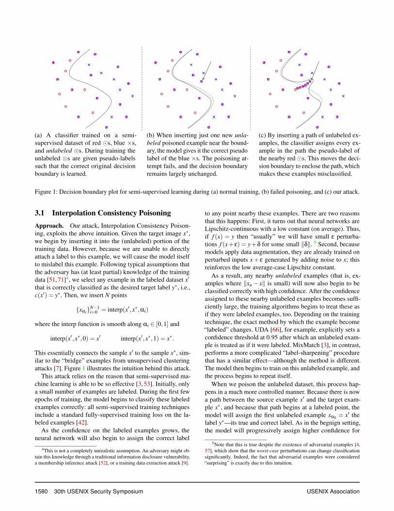
(a) A classifier trained on a semi-supervised dataset of red �s, blue ×s,and unlabeled ⊗s. During training theunlabeled ⊗s are given pseudo-labelssuch that the correct original decisionboundary is learned.

(b) When inserting just one new unla-beled poisoned example near the bound-ary, the model gives it the correct pseudolabel of the blue ×s. The poisoning at-tempt fails, and the decision boundaryremains largely unchanged.

(c) By inserting a path of unlabeled ex-amples, the classifier assigns every ex-ample in the path the pseudo-label ofthe nearby red �s. This moves the deci-sion boundary to enclose the path, whichmakes these examples misclassified.

Figure 1: Decision boundary plot for semi-supervised learning during (a) normal training, (b) failed poisoning, and (c) our attack.

3.1 Interpolation Consistency PoisoningApproach. Our attack, Interpolation Consistency Poison-ing, exploits the above intuition. Given the target image x∗,we begin by inserting it into the (unlabeled) portion of thetraining data. However, because we are unable to directlyattach a label to this example, we will cause the model itselfto mislabel this example. Following typical assumptions thatthe adversary has (at least partial) knowledge of the trainingdata [51, 71]4, we select any example in the labeled dataset x′

that is correctly classified as the desired target label y∗, i.e.,c(x′) = y∗. Then, we insert N points

{xαi}N−1i=0 = interp(x′,x∗,αi)

where the interp function is smooth along αi ∈ [0,1] and

interp(x′,x∗,0) = x′ interp(x′,x∗,1) = x∗.

This essentially connects the sample x′ to the sample x∗, sim-ilar to the “bridge” examples from unsupervised clusteringattacks [7]. Figure 1 illustrates the intuition behind this attack.

This attack relies on the reason that semi-supervised ma-chine learning is able to be so effective [3, 53]. Initially, onlya small number of examples are labeled. During the first fewepochs of training, the model begins to classify these labeledexamples correctly: all semi-supervised training techniquesinclude a standard fully-supervised training loss on the la-beled examples [42].

As the confidence on the labeled examples grows, theneural network will also begin to assign the correct label

4This is not a completely unrealistic assumption. An adversary might ob-tain this knowledge through a traditional information disclosure vulnerability,a membership inference attack [52], or a training data extraction attack [9].

to any point nearby these examples. There are two reasonsthat this happens: First, it turns out that neural networks areLipschitz-continuous with a low constant (on average). Thus,if f (x) = y then “usually” we will have small ε perturba-tions f (x+ ε) = y+δ for some small ‖δ‖. 5 Second, becausemodels apply data augmentation, they are already trained onperturbed inputs x+ ε generated by adding noise to x; thisreinforces the low average-case Lipschitz constant.

As a result, any nearby unlabeled examples (that is, ex-amples where ‖xu− x‖ is small) will now also begin to beclassified correctly with high confidence. After the confidenceassigned to these nearby unlabeled examples becomes suffi-ciently large, the training algorithms begins to treat these asif they were labeled examples, too. Depending on the trainingtechnique, the exact method by which the example become“labeled” changes. UDA [66], for example, explicitly sets aconfidence threshold at 0.95 after which an unlabeled exam-ple is treated as if it were labeled. MixMatch [3], in contrast,performs a more complicated “label-sharpening” procedurethat has a similar effect—although the method is different.The model then begins to train on this unlabeled example, andthe process begins to repeat itself.

When we poison the unlabeled dataset, this process hap-pens in a much more controlled manner. Because there is nowa path between the source example x′ and the target exam-ple x∗, and because that path begins at a labeled point, themodel will assign the first unlabeled example xα0 = x′ thelabel y∗—its true and correct label. As in the begnign setting,the model will progressively assign higher confidence for

5Note that this is true despite the existence of adversarial examples [4,57], which show that the worst-case perturbations can change classificationsignificantly. Indeed, the fact that adversarial examples were considered“surprising” is exactly due to this intuition.


this label on this example. Then, the semi-supervised learn-ing algorithms will encourage nearby samples (in particular,xα1) to be assigned the same label y∗ as the label given tothis first point xα0 . This process then repeats. The model as-signs higher and higher likelihood to the example xα1 to beclassified as y∗, which then encourages xα2 to become clas-sified as y∗ as well. Eventually all injected examples {xαi}will be labeled the same way, as y∗. This implies that finally,f (xα0) = f (xN−1) = f (x∗) = y∗ will be as well, completingthe poisoning attack.

Interpolation Strategy. It remains for us to instantiate thefunction interp. To begin we use the simplest strategy: linearpixel-wise blending between the original example x′ and thetarget example x∗. That is, we define

interp(x′,x∗,α) = x′ · (1−α)+ x∗ ·α.

This satisfies the constraints defined earlier: it is smooth, andthe boundary conditions hold. In Section 4.2 we will constructfar more sophisticated interpolation strategies (e.g., using aGAN [17] to generate semantically meaningful interpola-tions); for the remainder of this section we demonstrate theutility of a simpler strategy.

Density of poisoned samples. The final detail left to spec-ify is how we choose the values of αi. The boundary con-ditions α0 = 0 and αN−1 = 1 are fixed, but how should weinterpolate between these two extremes? The simplest strat-egy would be to sample completely linearly within the range[0,1], and set αi = i/N. This choice, though, is completelyarbitrary; we now define what it would look like to providedifferent interpolation methods that might allow for an attackto succeed more often.

Each method we consider works by first choosing a densityfunctions ρ(x) that determines the sampling rate. Given adensity function, we first normalize it

ρ(x) = ρ(x) ·(∫ 1

0ρ(x)dx

)−1

and then sample from it so that we sample α according to

Pr[p < α < q] =∫ q

pρ(x)dx.

For example, the function ρ(x) = 1 corresponds to a uni-form sampling of α in the range [0,1]. If we instead sampleaccording to ρ(x) = x then α will be more heavily samplednear 1 and less sampled near 0, causing more insertions nearthe target example and fewer insertions near the original ex-ample. Unless otherwise specified, in this paper we use thesampling function ρ(x) = 1.5− x. This is the function thatwe found to be most effective in an experiment across elevencandidate density functions—see Section 3.2.7 for details.

3.2 EvaluationWe extensively validate the efficacy of our proposed attacks onthree datasets and seven semi-supervised learning algorithms.

3.2.1 Experimental Setup

Datsets We evaluate our attack on three datasets typicallyused in semi-supervised learning:

• CIFAR-10 [29] is the most studied semi-supervisedlearning dataset, with 50,000 images from 10 classes.

• SVHN [41] is a larger dataset of 604,388 images ofhouse numbers, allowing us to evaluate the efficacy ofour attack on datasets with more examples.

• STL-10 [12] is a dataset designed for semi-supervisedlearning. It contains just 1,000 labeled images (at ahigher-resolution, 96×96), with an additional 100,000unlabeled images drawn from a similar (but not identical)distribution, making it our most realistic dataset.

Because CIFAR-10 and SVHN were initially designed forfully-supervised training, semi-supervised learning researchuses these dataset by discarding the labels of all but a smallnumber of examples—typically just 40 or 250.

Semi-Supervised Learning Methods We perform mostexperiments on the three most accurate techniques: Mix-Match [3], UDA [66], and FixMatch [53], with additionalexperiments on VAT [39], Mean Teacher [59], Pseudo La-bels [33], and Pi Model [31]. The first three methods listedabove are 3−10× more accurate compared to the next fourmethods. As a result we believe these will be most useful inthe future, and so focus on them.

We train all models with the same 1.4 million parameterResNet-28 [19] model that reaches 96.38% fully-supervisedaccuracy. This model has become the standard benchmarkmodel for semi-supervised learning [42] due to its relativesimplicity and small size while also reaching near state-of-the-art results [53]. In all experiments we confirm that poisoningthe unlabeled dataset maintains standard accuracy.

Experiment Setup Details. In each section below we an-swer several research questions; for each experimental trialwe perform 8 attack attempts and report the success rate. Ineach of these 8 cases, we choose a new random source imageand target image uniformly at random. Within each figure ortable we re-use the same randomly selected images to reducethe statistical noise of inter-table comparisons.

While it would clearly be preferable to run each experimentwith more than 8 trials, semi-superivsed machine learningalgorithms are extremely slow to train: one run of FixMatchtakes 20-GPU hours on CIFAR-10, and over five days on STL-10. Thus, with eight trials per experiment, our evaluationsrepresent hundreds of GPU-days of compute time.


Plane

Car Bird Cat DeerDog Fro

gHors

eSh

ipTru

ckAve

rage

Original Label of Poisoned Image

TruckShip

HorseFrogDog

DeerCatBirdCar

Plane

Average

Targ

et (D

esire

d) L

abel

for P

oiso

ned

Imag

e

0.0

0.2

0.4

0.6

0.8

1.0

Figure 2: Poisoning attack success rate averaged across theten CIFAR-10 classes. Each cell is the average of 16 trials.The original label of the (to-be-poisoned) image does notmake attacks (much) easier or harder, but some target labels(e.g., horse) are harder to reach than others (e.g., bird).

3.2.2 Preliminary Evaluation

We begin by demonstrating the efficacy of our attack on onemodel (FixMatch) on one dataset (CIFAR-10) for one poi-son ratio (0.1%). Further sections will perform additionalexperiments that expand on each of these dimensions. Whenwe run our attack eight different times with eight differentimage-label pairs, we find that it succeeds in seven of thesecases. However, as mentioend above, only performing eighttrials is limiting—maybe some images are easier or harderto successfully poison, or maybe some images are better orworse source images to use for the attack.

3.2.3 Evaluation across source- and target-image

In order to ensure our attack remains consistently effective,we now train an additional 40×40 models. For each model,we construct a different poison set by selecting 40 source(respectively, target) images from the training (testing) sets,with 4 images from each of the 10 classes.

We record each trial as a success if the target example endsup classified as the desired label—or failure if not. To reducetraining time, we remove half of the unlabeled examples (andmaintain a 0.1% poison ratio of the now-reduced-size dataset)and train for a quarter the number of epochs. Because we havereduced the total training, our attack success rate is reducedto 51% (future experiments will confirm the baseline >80%attack success rate found above).

Figure 2 gives the attack success rate broken down by thetarget image’s true (original) label, and the desired poison

Target (Test) Images

Sour

ce (L

abel

ed) I

mag

es

0.0

0.2

0.4

0.6

0.8

1.0

Figure 3: Poisoning attack success rate for all 40×40 source-target pairs; six (uniformly spaced) example images are shownon each axis. Each cell represents a single run of FixMatchpoisoning that source-target pair, and its color indicates if theattack succeeded (yellow) or failed (purple). The rows andcolumns are sorted by average attack success rate.

label. Some desired label such as “bird” or “cat” succeed in85% of cases, compared to the most difficult label of “horse”that succeeds in 25% of cases.

Perhaps more interesting than the aggregate statistics isconsidering the success rate on an image-by-image basis (seeFigure 3). Some images (e.g., in the first column) can rarelybe successfully poisoned to reach the desired label, whileother images (e.g., in the last column) are easily poisoned.Similarly, some source images (e.g., the last row) can poisonalmost any image, but other images (e.g., the top row) are poorsources. Despite several attempts, we have no explanation forwhy some images are easier or harder to attack.

3.2.4 Evaluation across training techniques

The above attack shows that it is possible to poison FixMatchon CIFAR-10 by poisoning 0.1% of the training dataset. Wenow broaden our argument by evaluating the attack successrate across seven different training techniques–but again forjust CIFAR-10. As stated earlier, in all cases the poisonedmodels retain their original test accuracy compared to thebenignly trained baseline on an unpoisoned dataset.

Figure 4 plots the main result of this experiment, whichcompares the accuracy of the final trained model to the poi-soning attack success rate. The three most recent methodsare all similarly vulnerable, with our attacks succeeding over80% of the time. When we train the four older techniques tothe highest test accuracy they can reach—roughly 60%—ourpoisoning attacks rarely succeed.


Dataset CIFAR-10 SVHN STL-10(% poisoned) 0.1% 0.2% 0.5% 0.1% 0.2% 0.5% 0.1% 0.2% 0.5%

MixMatch 5/8 6/8 8/8 4/8 5/8 5/8 4/8 6/8 7/8UDA 5/8 7/8 8/8 5/8 5/8 6/8 - - -FixMatch 7/8 8/8 8/8 7/8 7/8 8/8 6/8 8/8 8/8

Table 1: Success rate of our poisoning attack across datasets and algorithms, when poisoning between 0.1% and 0.5% ofthe unlabeled dataset. CIFAR-10 and SVHN use 40 labeled examples, and STL-10 all 1000. Our attack has a 67% success ratewhen poisoning 0.1% of the unlabeled dataset, and 91% at 0.5% of the unlabeled dataset (averaged across experiments).

0.0 0.2 0.4 0.6 0.8 1.0Mean (CIFAR-10) Model Accuracy

0.0

0.2

0.4

0.6

0.8

1.0

Atta

ck S

ucce

ss R

ate

(CIF

AR-1

0) FixMatchUDAMixMatchVATMeanTeacherPseudoLabelPiModel

Figure 4: More accurate techniques are more vulnerable.Success rate of poisoning CIFAR-10 with 250 labeled exam-ples and 0.2% poisoning rate. Each point averages ten trainedmodels. FixMatch, UDA, and MixMatch were trained undertwo evaluation settings, one standard (to obtain high accuracy)and one small-model to artificially reduce model accuracy.

This leaves us with the question: why does our attack workless well on these older methods? Because it is not possi-ble to artificially increase the accuracy of worse-performingtechniques, we artificially decrease the accuracy of the state-of-the-art techniques. To do this, we train FixMatch, UDA,and MixMatch for fewer total steps of training using a slightlysmaller model in order to reduce their final accuracy to be-tween 70−80%. This allows us correlate the techniques ac-curacy with its susceptibility to poisoning.

We find a clear relationship between the poisoning suc-cess rate and the technique’s accuracy. We hypothesize thisis caused by the better techniques extracting more “mean-ing” from the unlabeled data. (It is possible that, because weprimarily experimented with recent techniques, we have im-plicitly designed our attack to work better on these techniques.We believe the simplicity of our attack makes this unlikely.)This has strong implications for the future. It suggests thatdeveloping better training techniques is unlikely to preventpoisoning attacks—and will instead make the problem worse.

Dataset CIFAR-10 SVHN(# labels) 40 250 4000 40 250 4000

MixMatch 5/8 4/8 1/8 6/8 4/8 5/8UDA 5/8 5/8 2/8 5/8 4/8 4/8FixMatch 7/8 7/8 7/8 7/8 6/8 7/8

Table 2: Success rate of our attack when poisoning 0.1% ofthe unlabeled dataset when varying the number of labeledexamples in the dataset. Models provided with more labelsare often (but not always) more robust to attack.

3.2.5 Evaluation across datasets

The above evaluation considers only one dataset at one poi-soning ratio; we now show that this attack is general acrossthree datasets and three poisoning ratios.

Table 1 reports results for FixMatch, UDA, and MixMatch,as these are the methods that achieve high accuracy. (We omitUDA on STL-10 because it was not shown effective on thisdataset in [66].) Across all datasets, poisoning 0.1% of theunlabeled data is sufficient to successfully poison the modelwith probability at least 50%. Increasing the poisoning ratiobrings the attack success rate to near-100%.

As before, we find that the techniques that perform betterare consistently more vulnerable across all experiment setups.For example, consider the poisoning success rate on SVHN.Here again, FixMatch is more vulnerable to poisoning, withthe attack succeeding in aggregate for 20/24 cases comparedto 15/24 for MixMatch.

3.2.6 Evaluation across number of labeled examples

Semi-supervised learning algorithms can be trained with avarying number of labeled examples. When more labels areprovided, models typically perform more accurately. We nowinvestigate to what extent introducing more labeled examplesimpacts the efficacy of our poisoning attack. Table 2 summa-rizes the results. Notice that our prior observation comparingtechnique accuracy to vulnerability does not imply more ac-curate models are more vulnerable—with more training data,models are able to learn with less guesswork and so becomeless vulnerable.


CIFAR-10 % PoisonedDensity Function 0.1% 0.2% 0.5%

(1− x)2 0/8 3/8 7/8φ(x+ .5) 1/8 5/8 7/8φ(x+ .3) 2/8 7/8 8/8x 3/8 4/8 6/8x4 +(1− x)4 3/8 5/8 8/8√

1− x 3/8 6/8 6/8x2 +(1− x)2 4/8 5/8 8/81 4/8 6/8 8/8(1− x)2 + .5 5/8 7/8 8/81− x 5/8 8/8 8/81.5− x 7/8 8/8 8/8

Table 3: Success rate of poisoning a semi-supervised machinelearning model using different density functions to interpolatebetween the labeled example x′ (when α = 0) and the targetexample x∗ (when α = 1). Higher values near 0 indicate amore dense sampling near x′ and higher values near 1 indicatea more dense sampling near x∗. Experiments conducted withFixMatch on CIFAR-10 using 40 labeled examples.

3.2.7 Evaluation across density functions

All of the prior (and future) experiments in this paper usethe same density function ρ(·). In this section we evaluatedifferent choices to understand how the choice of functionimpacts the attack success rate.

Table 3 presents these results. We evaluate each samplingmethod across three different poisoning ratios. As a generalrule, the best sampling strategies sample slightly more heavilyfrom the source example, and less heavily from the target thatwill be poisoned. The methods that perform worst do notsample sufficiently densely near either the source or targetexample, or do not sample sufficiently near the middle.

For example, when we run our attack with the functionρ(x) = (1−x)2, then we sample frequently around the sourceimage x′, but infrequently around the target example x∗. Asa result, this density function fails at poisoning x∗ almostalways, because the density near x∗ is not high enough forthe model’s consistency regularization to take hold. We findthat the label successfully propagates almost all the way tothe final instance (to approximately α = .9) but the attackfails to change the classification of the final target example.Conversely, for a function like ρ(x) = x, the label propagationusually fails near α = 0, but whenever it succeed at gettingpast α > .25 then it always succeeds at reaching α = 1.

Experimentally the best density function we identifiedwas ρ(x) = 1.5− x, which samples three times more heavilyaround the source example x′ than around the target x∗.

α = 0.0 α = 1.0

0 20 40 60 80 100Training iteration

1.0

0.8

0.6

0.4

0.2

0.0Conf

iden

ce in

poi

sone

d la

bel

α= 0.00α= 0.25α= 0.50α= 0.75α= 1.00

Figure 5: Label propagation of a poisoning attack over train-ing epochs. The classifier begins by classifying the correctly-labeled source example x′ (when α = 0; image shown in theupper left) as the poisoned label. This propagates to the in-terpolation α > 0 one by one, and eventually on to the finalexample x∗ (when α = 1; image shown in the upper right).

3.3 Why does this attack work?Earlier in this section, and in Figure 1, we provided visualintuition why we believed our attack should succeed. If ourintuition is correct, we should expect two properties:

1. As training progresses, the confidence of the model oneach poisoned example should increase over time.

2. The example α0 = 0 should become classified as thetarget label first, followed by α1, then α2, on to αN = 1.

We validate this intuition by saving all intermediate modelpredictions after every epoch of training. This gives us a col-lection of model predictions for each epoch, for each poisonedexample in the unlabeled dataset.

In Figure 5, we visualize the predictions across a single Fix-Match training run.6 Initially, the model assigns all poisonedexamples 10% probability (because this is a ten-class clas-sification problem). After just ten epochs, the model beginsto classify the example α = 0 correctly. This makes sense:α = 0 is an example in the labeled dataset and so it shouldbe learned quickly. As α = 0 begins to be learned correctly,this prediction propagates to the samples α > 0. In particular,the example α = .25 (as shown) begins to become labeled asthe desired target. This process continues until the poisonedexample x∗ (where α = 1) begins to become classified as thepoisoned class label at epoch 80. By the end of training, allpoisoned examples are classified as the desired target label.

6Shown above are the poisoned samples. While blended images may lookout-of-distribution, Section 4.2 develops techniques to alleviate this.


4 Extending the Poisoning Attack

Interpolation Consistency Poisoning is effective at poisoningsemi-supervised machine learning models under this baselinesetup, but there are many opportunities for extending thisattack. Below we focus on three extensions that allow us to

1. attack without knowledge of any training datapoints,

2. attack with a more general interpolation strategy, and

3. attack transfer learning and fine-tuning.

4.1 Zero-Knowledge Attack

Our first attack requires the adversary knows at least oneexample in the labeled dataset. While there are settings wherethis is realistic [52], in general an adversary might have noknowledge of the labeled training dataset. We now developan attack that removes this assumption.

As an initial experiment, we investigate what would happenif we blindly connected the target point x∗ with an arbitraryexample x′ (not already contained within the labeled trainingdataset). To do this we mount exactly our earlier attack with-out modification, interpolating between an arbitrary unlabeledexample x′ (that should belong to class y∗, despite this labelnot being attached), and the target example x∗.

As we should expect, across all trials, when we connectdifferent source and target examples the trained model consis-tently labels both x′ and x∗ as the same final label. Unexpect-edly, we found that while the final label the model assignedwas rarely y∗ = c(x′) (our attack objective label), and insteadmost often the final label was a label neither y∗ nor c(x∗).

Why should connecting an example with label c(x′) andanother example with label c(x∗) result in a classifier that as-signs neither of these two labels? We found that the reason thishappens is that, by chance, some intermediate image xα willexceed the confidence threshold. Once this happens, both xα1

and xαN−1 become classified as however xα was classified—which often is not the label as either endpoint.

In order to better regularize the attack process we provideadditional support. To do this, we choose additional images{xi} and then connect each of these examples to x′ with apath, blending as we do with the target example.

These additional interpolations make it more likely for x′ tobe labeled correctly as y∗, and when this happens, then morelikely that the attack will succeed.

Evaluation Table 6 reports the results of this poisoningattack. Our attack success rate is lower, with roughly halfof attacks succeeding at 1% of training data poisoned. Allof these attacks succeed at making the target example x∗

becoming mislabeled (i.e., f (x∗) 6= c(x∗)) even though it isnot necessary labeled as the desired target label.

Dataset CIFAR-10 SVHN(% poisoned) 0.5% 1.0% 0.5% 1.0%

MixMatch 2/8 4/8 3/8 4/8UDA 2/8 3/8 4/8 4/8FixMatch 3/8 4/8 3/8 5/8

Figure 6: Success rate of our attack at poisoning the unlabeleddataset without knowledge of any training examples. As inTable 1, experiments are across three algorithms, but hereacross two datasets.

4.2 Generalized Interpolation

When performing linear blending between the source andtarget example, human visual inspection of the poisoned ex-amples could identify them as out-of-distribution. While itmay be prohibitively expensive for a human to label all of theexamples in the unlabeled dataset, it may not be expensiveto discard examples that are clearly incorrect. For example,while it may take a medical professional to determine whethera medical scan shows signs of some disease, any human couldreject images that were obviously not medical scans.

Fortunately there is more than one way to interpolate be-tween the source example x′ and the target example x∗. Earlierwe used a linear pixel-space interpolation. In principle, anyinterpolation strategy should remain effective—we now con-sider an alternate interpolation strategy as an example.

Making our poisoning attack inject samples that are notoverly suspicious therefore requires a more sophisticated inter-polation strategy. Generative Adversarial Networks (GANs)[17] are neural networks designed to generate synthetic im-ages. For brevity we omit details about training GANs as ourresults are independent of the method used. The generator ofa GAN is a function g : Rn→ X , taking a latent vector z∈Rn

and returning an image. GANs are widely used because oftheir ability to generate photo-realistic images.

One property of GANs is their ability to perform semanticinterpolation. Given two latent vectors z1 and z2 (for example,latent vectors corresponding to a picture of person facing leftand a person facing right), linearly interpolating between z1and z2 will semantically interpolate between the two images(in this case, by rotating the face from left to right).

For our attack, this means that it is possible to take our twoimages x′ and x∗, compute the corresponding latent vectorsz′ and z∗ so that G(z′) = x′ and G(z∗) = x∗, and then linearlyinterpolate to obtain xi = G((1−αi)z′+αiz∗). There is onesmall detail: in practice it is not always possible to obtaina latent vector z′ so that exactly G(z′) = x′ holds. Instead,the best we can hope for is that ‖G(z′)− x′‖ is small. Thus,we perform the attack as above interpolating between G(z′)and G(z∗) and then finally perform the small interpolationbetween x′ and G(z′), and similarly x∗ and G(z∗).


Evaluation. We use a DC-GAN [46] pre-trained on CIFAR-10 to perform the interpolations. We again perform the sameattack as above, where we poison 1% of the unlabeled exam-ples by interpolating in between the latent spaces of z′ and z∗.Our attack succeeds in 9 out of 10 trials. This slightly reducedattack success rate is a function of the fact that while the twoimages are similarly far apart, the path taken is less direct.

4.3 Attacking Transfer LearningOften models are not trained from scratch but instead ini-tialized from the weights of a different model, and then finetuned on additional data [43]. This is done either to speed uptraining via “warm-starting”, or when limited data is available(e.g., using ImageNet weights for cancer detection [15]).

Fine-tuning is known to make attacks easier. For example,if it’s public knowledge that a model has been fine-tuned froma particular ImageNet model, it becomes easier to generate ad-versarial examples on the fine-tuned model [63]. Similarly, ad-versaries might attempt to poison or backdoor a high-qualitysource model, so that when a victim uses it for transfer learn-ing their model becomes compromised as well [68].

Consistent with prior work we find that it is easier to poisonmodels that are initialized from a pretrained model [51]. Theintuition here is simple. The first step of our standard attackswaits for the model to assign x′ the (correct) label y∗ before itcan propagate to the target label f (x∗) = y∗. If we know theinitial model weights θinit, then we can directly compute

x′ = arg minδ : fθinit (x

∗+δ)=y∗‖δ‖.

That is, we search for an example x′ that is nearby the desiredtarget x∗ so that the initial model fθinit already assigns examplex′ the label y∗. Because this initial model assigns x′ the labely∗, then the label will propagate to x∗—but because the twoexamples are closer, the propagation happens more quickly.

Evaluation We find that this attack is even more effectivethan our baseline attack. We initialize our model with a semi-supervised learning model trained on the first 50% of theunlabeled dataset to convergence. Then, we provide this ini-tial model weights θinit to the adversary. The adversary solvesthe minimization formulation above using standard gradientdescent, and then interpolates between that x′ and the samerandomly selected x∗. Finally, the adversary inserts poisonedexamples into the second 50% of the unlabeled dataset, modi-fying just 0.1% of the unlabeled dataset.

We resume training on this additional clean data (alongwith the poisoned examples). We find that, very quickly, thetarget example becomes successfully poisoned. This matchesour expectation: because the distance between the two exam-ples is very small, the model’s decision boundary does nothave to change by much in order to cause the target exampleto become misclassified. In 8 of 10 trials, this attack succeeds.

4.4 Negative ResultsWe attempted five different extensions of our attack that didnot work. Because we believe these may be illuminating, wenow present each of these in turn.

Analytically computing the optimal density function InTable 3 we studied eleven different density functions. Initially,we attempted to analytically compute the optimal densityfunction, however this did not end up succeeding. Our firstattempt repeatedly trained classifiers and performed binarysearch to determine where along the bridge to insert newpoisoned examples. We also started with a dense interpolationof 500 examples, and removed examples while the attacksucceeded. Finally, we also directly computed the maximumdistance ε so that training on example u would cause theconfidence of u+δ (for ‖δ‖2 = ε) to increase.

Unfortunately, each of these attempts failed for the samereason: the presence or absence of one particular example isnot independent of the other examples. Therefore, it is difficultto accurately measure the true influence of any particularexample, and greedy searches typically got stuck in localminima that required more insertions than just a constantinsertion density with fewer starting examples.

Multiple intersection points Our attack chooses onesource x′ and connects a path of unlabeled examples from thatsource x′ to the target x∗. However, suppose instead that weselected multiple samples {x′i}n

i=1 and then constructed pathsfrom each x′i to x∗. This might make it appear more likely tosucceed: following the same intuition behind our “additionalsupport” attack, if one of the paths breaks, one of the otherpaths might still succeed.

However, for the same insertion budget, experimentally wefind it is always better to use the entire budget on one singlepath from x′ to x∗ than to spread it out among multiple paths.

Adding noise to the poisoned examples When interpolat-ing between x′ and x∗ we experimented with adding point-wise Gaussian or uniform noise to xα. Because images arediscretized into {0,1, . . . ,255}hwc, it is possible that two suf-ficiently close α,α′ will have discretize(xα) = discretize(xα′)even though xα 6= xα′ . By adding a small amount of noise,this property is no longer true, and therefore the model willnot see the same unlabeled example twice.

However, doing this did not improve the efficacy of the at-tack for small values of σ, and made it worse for larger valuesof σ. Inserting the same example into the unlabeled datasettwo times was more effective than just one time, because themodel trains on that example twice as often.

Increasing attack success rate. Occasionally, our attackgets “stuck”, and x′ becomes classified as y∗ but x∗ does not.When this happens, the poisoned label only propagates part


of the way through the bridge of poisoned examples. That is,for some threshold t, we have that xi<t = y∗ but for xi>t 6= y∗.Even if t = 0.9, and the propagation has made it almost allthe way to the final label, past a certain time in training themodel’s label assignments become fixed and the predictedlabels no longer change. It would be interesting to betterunderstand why these failures occur.

Joint labeled and unlabeled poisoning. Could our attackimprove if we gave the adversary the power to inject a sin-gle, correctly labeled, poisoned example (as in a clean-labelpoisoning attack)? We attempted various strategies to do this,ranging from inserting out-of-distribution data [48] to mount-ing a Poison Frog attack [51]. However, none of these ideasworked better than just choosing a good source example asdetermined in Figure 3. Unfortunately, we currently do nothave a technique to predict which samples will be good orbad sources (other than brute force training).

5 Defenses

We now shift our focus to preventing the poisoning attack wehave just developed. While we believe existing defense arenot well suited to defend against our attacks, we believe thatby combining automatic techniques to identify potentially-malicious examples, and then manually reviewing these lim-ited number of cases, it may be possible to prevent this attack.

5.1 General-Purpose Poisoning Defenses

While there are a large class of defenses to indiscriminatepoisoning attacks [8, 11, 22, 23, 56], there are many fewerdefenses that prevent the targeted poisoning attacks we study.We briefly consider two defenses here.

Fine-tuning based defenses [34] take a (potentially poi-soned) model and fine-tune it on clean, un-poisoned data.These defenses hope (but can not guarantee) that doing thiswill remove any unwanted memorization of the model. Inprinciple these defenses should work as well on our settingas any other if there is sufficient data available—however,because semi-supervised learning was used in the first case, itis unlikely there will exist a large, clean, un-poisoned dataset.

Alternatively, other defenses [20] alter the training processto apply differentially private SGD [1] in order to mitigate theability of the model to memorize training examples. However,because the vulnerability of this defense scales exponentiallywith the number of poisoned examples, these defenses areonly effective at preventing extremely limited poisoning at-tacks that insert fewer than three or five examples.

Our task and threat model are sufficiently different fromthese prior defenses that they are a poor fit for our problemdomain: the threat models do not closely align.

5.2 Dataset Inspection & Cleaning

We now consider two defenses tailored specifically to preventour attacks. While it is undesirable to pay a human to manu-ally inspect the entire unlabeled dataset (if this was acceptablethen the entire dataset might as well be labeled), this does notpreclude any human review. Our methods directly process theunlabeled dataset and filter out a small subset of the examplesto have reviewed by a human for general correctness (e.g.,“does this resemble anything like a dog?” compared to “whichof the 100+ breeds of dog in the ImageNet dataset is this?”).

Detecting pixel-space interpolations Our linear imageblending attack is trivially detectable. Recall that for thisattack we set xαi = (1−αi) · x′+αi · x∗. Given the unlabeleddataset U, this means that there will exist at least three ex-amples u,v,w ∈ U that are colinear in pixel space. For ourdataset sizes, a trivial trial-and-error sampling identifies thepoisoned examples in under ten minutes on a GPU. Whileeffective for this particular attack, it can not, for example,detect our GAN latent space attack.

We can improve on this to detect arbitrary interpolations.Agglomerative Clustering [64] creates clusters of similar ex-amples (under a pixel-space `2 norm, for example). Initiallyevery example is placed into its own set. Then, after comput-ing the pairwise distance between all sets, the two sets withminimal distance are merged to form one set. The processrepeats until the smallest distance exceeds some threshold.

Because our poisoned examples are all similar in pixel-space to each other, it is likely that they will be all placed inthe same cluster. Indeed, running a standard implementationof agglomerative clustering [45] is effective at identifyingthe poisoned examples in our attacks. Thus, by removing thelargest cluster, we can completely prevent this attack.

The inherent limitation of this defenses is that it assumethat the defender can create a useful distance function. Using`2 distance above worked because our attack performed pixel-space blending. However, if the adversary inserted examplesthat applied color-jitter, or small translations, this defensewould no longer able to identify the cluster of poisoned ex-amples. This is a cat-and-mouse game we want to avoid.

5.3 Monitoring Training Dynamics

Unlike the prior defenses that inspect the dataset directly todetect if an example is poisoned or not, we now develop asecond strategy that predicts if an example is poisoned byhow it impacts the training process.

Recall the reason our attack succeeds: semi-supervisedlearning slowly grows the correct decision boundary out fromthe initial labeled examples towards the “nearest neighbors”in the unlabeled examples, and continuing outwards. Theguessed label of each unlabeled example will therefore beinfluenced by (several) other unlabeled examples. For benign


examples in the unlabeled set, we should expect that they willbe influenced by many other unlabeled examples simultane-ously, of roughly equal importance. However, by construction,our poisoned examples are designed to predominantly impactthe prediction of the other poisoned examples—and not beaffected by, or affect, the other unlabeled examples.

We now construct a defense that relies on this observation.By monitoring the training dynamics of the semi-supervisedlearning algorithm, we isolate out (and then remove) thoseexamples that are influenced by only a few other examples.

Computing pairwise influence What does it mean for oneexample to influence the training of another example? Inthe context of fully-supervised training, there are rigorousdefinitions of influence functions [28] that allow for one to(somewhat) efficiently compute the training examples thatmaximally impacted a given prediction. However, our influ-ence question has an important difference: we ask not whattraining points influenced a given test point, but what (unla-beled) training points influenced another (unlabeled) trainingpoint. We further find that it is not necessary to resort tosuch sophisticated approaches, and a simpler (and 10−100×faster) method is able to effectively recover influence.

While we can not completely isolate out correlation andcausation without modifying the training process, we makethe following observation that is fundamental to this defense:

If example u influences example v, thenwhen the prediction of u changes, the pre-diction of v should change in a similar way.

After every epoch of training, we record the model’s pre-dictions on each unlabeled example. Let fθi(u j) denote themodel’s prediction vector after epoch i on the jth unlabeledexample. For example, in a binary decision task, if at epoch 6the model assigns example u5 class 0 with probability .7 andclass 1 with .3, then fθ6(u5) =

[.7 .3

]. From here, define

∂ fθi(u j) = fθi+1(u j)− fθi(u j)

with subtraction taken component-wise. That is, ∂ f representsthe difference in the models predictions on a particular exam-ple from one epoch to the next. This allows us to formallycapture the intuition for “the prediction changing”.

Then, for each example, we let

µ(a,b)j =[∂ fθa(u j) ∂ fθa+1(u j) . . . ∂ fθb−1(u j) fθb(u j)

]be the model’s collection of prediction deltas from epoch a toepoch b. We compute the influence of example ui on u j as

Influence(ui,u j) = ‖µ(0,K−2)i −µ(1,K−1)

j ‖22.

That is, example ui influences example u j if when exam-ple ui makes a particular change at epoch k, then exampleu j makes a similar change in the next epoch—because it has

10−5 10−4 10−3 10−2 10−1 100

Mean Influence of 5 Nearest Neighbors

100

101

102

103

Freq

uenc

y (lo

g sc

aled

)

Benign ExamplesPoisoned Examples

Figure 7: Our training-dynamics defense perfectly separatesthe inserted poisoned examples from the benign unlabeledexamples on CIFAR-10 for a FixMatch poisoned model. Plot-ted is the frequency of the influence value across the unla-beled examples. Benign unlabeled examples are not heavilyinfluenced by their nearest neighbors (indicated by the highvalues), but poisoned examples are highly dependent on theother poisoned examples (indicated by the low values).

been influenced by ui. This definition of influence is clearlya simplistic approximation, and is unable to capture sophisti-cated relationships between examples. We nevertheless findthat this definition of influence is useful.

Identifying poisoned examples For each example in theunlabeled training set, we compute the average influence ofthe 5 nearest neighbors

avg influence(u) =15 ∑

v∈UInfluence(u,v) ·1[close5(u,v)]

where close5(u,v) is true if v is one of the 5 closest (by in-fluence) neighbors to u. (Our result is not sensitive to thearbitrary choice of 5; values from 2 to 10 perform similarly.)

Results. This technique perfectly separates the clean andpoisoned examples for each task we consider. In Figure 7we plot a representative histogram of influence values forbenign and poisoned examples; here we train a FixMatchmodel poisoning 0.2% of the CIFAR-10 dataset and 40 la-beled examples. The natural data is well-clustered with anaverage influence of 2 ·10−2, and the injected poisoned exam-ples all have an influence lower than 2 ·10−4, with a mean of3 ·10−5. Appendix B shows 8 more plots for additional runsof FixMatch and MixMatch on CIFAR-10, and SVHN.

When the attack itself fails to poison the target class, it isstill possible to identify all of the poisoned examples that havebeen inserted (i.e., with a true positive rate of 100%), but the


Figure 8: Our defenses’s near false positives are dupli-cated images. The left-most column contains five imagesfrom the CIFAR-10 unlabeled dataset that our defense iden-tifies as near false positives. At right are the four next-most-similar images from the CIFAR-10 unlabeled set as computedby our average influence definition. All of these similar im-ages are visual (near-)duplicates of the first.

false positive rate increases slightly to 0.1%. In practice, allthis means the defender should collect a few percent moreunlabeled examples more than are required so that any mali-cious examples can be removed. Even if extra training data isnot collected, training on 99.9% of the unlabeled dataset withthe false positives removed does not statistically significantlyreduce clean model accuracy.

Thus, at cost of doubling the training time—training oncewith poisoned examples, and a second time after removingthem—it is possible to completely prevent our attack. Multi-ple rounds of this procedure might improve its success ratefurther if not all examples can be removed in one iteration.

Examining (near) false positives. Even the near false pos-itives of our defense are insightful to analyze. In Figure 8 weshow five (representative) images of the benign examples inthe CIFAR-10 training dataset that our defense almost rejectsas if they were poisoned examples.

Because these examples are all nearly identical, they heav-ily influence each other according to our definition. When oneexamples prediction changes, the other examples predictionsare likely to change as well. This also explains why removingnear-false-positives does not reduce model accuracy.

Counter-attacks to these defenses. No defense is full-proof, and this defense is no different. It is likely that futureattacks will defeat this defense, too. However, we believe thatdefenses of this style are a promising direction that (a) serveas a strong baseline for defending against unlabeled datasetpoisoning attacks, and (b) could be extended in future work.

6 Conclusion

Within the past years, semi-supervised learning has gone from“completely unusable” [61] to nearly as accurate as the fully-supervised baselines despite using 100× less labeled data.However, using semi supervised learning in practice will re-quire understanding what new vulnerabilities will arise as aresult of training on this under-specified problem.

In this paper we study the ability for an adversary to poisonsemi-supervised learning algorithms by injecting unlabeleddata. As a result of our attacks, production systems will notbe able to just take all available unlabeled data, feed it intoa classifier, and hope for the best. If this is done, an adver-sary will be able to cause specific, targeted misclassifications.Training semi-supervised learning algorithms on real-worlddata will require defenses tailored to preventing poisoningattacks whenever collecting data from untrusted sources.

Surprisingly, we find that more accurate semi-supervisedlearning methods are more vulnerable to poisoning attacks.Our attack never succeeds on MeanTeacher because it has a50% error rate on CIFAR-10; in contrast, FixMatch reaches a5% error rate and as a result is easily poisoned. This suggeststhat simply waiting for more accurate methods not only won’tsolve the problem, but may even make the problem worse asfuture methods become more accurate.

Defending against poisoning attacks also can not beachieved through extensive use of human review—doing sowould reduce or eliminate the only reason to apply semi-supervised learning in the first place. Instead, we study de-fenses that isolate a small fraction of examples that should bereviewed or removed. Our defenses are effective at preventingthe poisoning attack we present, and we believe it will providea strong baseline by which future work can be evaluated.

More broadly, we believe that or analysis highlights thatthe recent trend where machine learning systems are trainedon any and all available data, without regard to its quality ororigin, might introduce new vulnerabilities. Similar trendshave recently been observed in other domains; for example,neural language models trained on unlabeled data scrapedfrom the Internet can be poisoned to perform targeted mis-predictions [49]. We expect that other forms of unlabeledtraining, such as self -supervised learning, will be similarlyvulnerable to these types of attacks. We hope our analysiswill allow future work to perform additional study of thisphenomenon in other settings where uncurated data is used totrain machine learning models.

Acknowledgements

We are grateful to Andreas Terzis, David Berthelot, and theanonymous reviewers for the discussion, suggestions, andfeedback that significantly improved this paper.


References[1] M. Abadi, A. Chu, I. Goodfellow, H. B. McMahan, I. Mironov, K. Tal-

war, and L. Zhang, “Deep learning with differential privacy,” in Pro-ceedings of the 2016 ACM SIGSAC Conference on Computer andCommunications Security, 2016, pp. 308–318.

[2] M. Barreno, B. Nelson, R. Sears, A. D. Joseph, and J. D. Tygar, “Canmachine learning be secure?” in Proceedings of the 2006 ACM Sympo-sium on Information, computer and communications security, 2006.

[3] D. Berthelot, N. Carlini, I. Goodfellow, N. Papernot, A. Oliver, and C. A.Raffel, “Mixmatch: A holistic approach to semi-supervised learning,”in Advances in Neural Information Processing Systems, 2019.

[4] B. Biggio, I. Corona, D. Maiorca, B. Nelson, N. Šrndic, P. Laskov,G. Giacinto, and F. Roli, “Evasion attacks against machine learningat test time,” in Joint European conference on machine learning andknowledge discovery in databases. Springer, 2013, pp. 387–402.

[5] B. Biggio, B. Nelson, and P. Laskov, “Poisoning attacks against supportvector machines,” 2012.

[6] B. Biggio, I. Pillai, S. Rota Bulò, D. Ariu, M. Pelillo, and F. Roli, “Isdata clustering in adversarial settings secure?” in Proceedings of the2013 ACM workshop on Artificial intelligence and security, 2013.

[7] B. Biggio, K. Rieck, D. Ariu, C. Wressnegger, I. Corona, G. Giacinto,and F. Roli, “Poisoning behavioral malware clustering,” in Proceedingsof the 2014 workshop on artificial intelligent and security workshop,2014, pp. 27–36.

[8] E. J. Candès, X. Li, Y. Ma, and J. Wright, “Robust principal componentanalysis?” Journal of the ACM (JACM), vol. 58, no. 3, pp. 1–37, 2011.

[9] N. Carlini, C. Liu, Ú. Erlingsson, J. Kos, and D. Song, “The secretsharer: Evaluating and testing unintended memorization in neural net-works,” in 28th USENIX Security Symposium (USENIX Security 19),2019, pp. 267–284.

[10] X. Chen, C. Liu, B. Li, K. Lu, and D. Song, “Targeted backdoor at-tacks on deep learning systems using data poisoning,” arXiv preprintarXiv:1712.05526, 2017.

[11] Y. Chen, C. Caramanis, and S. Mannor, “Robust sparse regressionunder adversarial corruption,” in International Conference on MachineLearning, 2013.

[12] A. Coates, A. Ng, and H. Lee, “An analysis of single-layer networksin unsupervised feature learning,” in Proceedings of the fourteenthinternational conference on artificial intelligence and statistics, 2011,pp. 215–223.

[13] E. D. Cubuk, B. Zoph, D. Mane, V. Vasudevan, and Q. V. Le, “Autoaug-ment: Learning augmentation strategies from data,” in Proceedings ofthe IEEE Conference on Computer Vision and Pattern Recognition,2019.

[14] T. DeVries and G. W. Taylor, “Improved regularization of convolutionalneural networks with cutout,” arXiv preprint arXiv:1708.04552, 2017.

[15] A. Esteva, B. Kuprel, R. A. Novoa, J. Ko, S. M. Swetter, H. M. Blau,and S. Thrun, “Dermatologist-level classification of skin cancer withdeep neural networks,” Nature, vol. 542, no. 7639, pp. 115–118, 2017.

[16] R. Geirhos, J.-H. Jacobsen, C. Michaelis, R. Zemel, W. Brendel,M. Bethge, and F. A. Wichmann, “Shortcut learning in deep neuralnetworks,” in Nat Mach Intell 2, 2020, pp. 665—-673.

[17] I. Goodfellow, J. Pouget-Abadie, M. Mirza, B. Xu, D. Warde-Farley,S. Ozair, A. Courville, and Y. Bengio, “Generative adversarial nets,” inAdvances in Neural Information Processing Systems, 2014.

[18] T. Gu, B. Dolan-Gavitt, and S. Garg, “Badnets: Identifying vulnerabil-ities in the machine learning model supply chain,” in Proceedings ofthe NIPS Workshop on Mach. Learn. and Comp. Sec, 2017.

[19] K. He, X. Zhang, S. Ren, and J. Sun, “Deep residual learning for imagerecognition,” in Proceedings of the IEEE conference on computer visionand pattern recognition, 2016, pp. 770–778.

[20] S. Hong, V. Chandrasekaran, Y. Kaya, T. Dumitras, and N. Papernot,“On the effectiveness of mitigating data poisoning attacks with gradientshaping,” arXiv preprint arXiv:2002.11497, 2020.

[21] A. Ilyas, S. Santurkar, D. Tsipras, L. Engstrom, B. Tran, and A. Madry,“Adversarial examples are not bugs, they are features,” in Advances inNeural Information Processing Systems, 2019, pp. 125–136.

[22] M. Jagielski, A. Oprea, B. Biggio, C. Liu, C. Nita-Rotaru, and B. Li,“Manipulating machine learning: Poisoning attacks and countermea-sures for regression learning,” in 2018 IEEE Symposium on Securityand Privacy (SP). IEEE, 2018, pp. 19–35.

[23] M. Kearns and M. Li, “Learning in the presence of malicious errors,”SIAM Journal on Computing, vol. 22, no. 4, pp. 807–837, 1993.

[24] N. S. Keskar, D. Mudigere, J. Nocedal, M. Smelyanskiy, and P. T. P.Tang, “On large-batch training for deep learning: Generalization gapand sharp minima,” International Conference on Learning Representa-tions, 2017.

[25] D. P. Kingma and J. Ba, “Adam: A method for stochastic optimization,”International Conference on Learning Representations, 2015.

[26] M. Kloft and P. Laskov, “Online anomaly detection under adversarialimpact,” in Proceedings of the thirteenth international conference onartificial intelligence and statistics, 2010, pp. 405–412.

[27] ——, “Security analysis of online centroid anomaly detection,” TheJournal of Machine Learning Research, vol. 13, no. 1, 2012.

[28] P. W. Koh and P. Liang, “Understanding black-box predictions via in-fluence functions,” in Proceedings of the 34th International Conferenceon Machine Learning-Volume 70. JMLR. org, 2017, pp. 1885–1894.

[29] A. Krizhevsky, G. Hinton et al., “Learning multiple layers of featuresfrom tiny images,” (Technical Report), 2009.

[30] A. Krogh and J. A. Hertz, “A simple weight decay can improve gen-eralization,” in Advances in Neural Information Processing Systems,1992, pp. 950–957.

[31] S. Laine and T. Aila, “Temporal ensembling for semi-supervised learn-ing,” International Conference on Learning Representations, 2017.

[32] Y. LeCun, Y. Bengio, and G. Hinton, “Deep learning,” nature, vol. 521,no. 7553, pp. 436–444, 2015.

[33] D.-H. Lee, “Pseudo-label: The simple and efficient semi-supervisedlearning method for deep neural networks,” in Workshop on challengesin representation learning, ICML, vol. 3, 2013, p. 2.

[34] K. Liu, B. Dolan-Gavitt, and S. Garg, “Fine-pruning: Defending againstbackdooring attacks on deep neural networks,” in International Sym-posium on Research in Attacks, Intrusions, and Defenses. Springer,2018, pp. 273–294.

[35] X. Liu, S. Si, X. Zhu, Y. Li, and C.-J. Hsieh, “A unified frameworkfor data poisoning attack to graph-based semi-supervised learning,”Advances in Neural Information Processing Systems, 2020.

[36] Y. Liu, X. Ma, J. Bailey, and F. Lu, “Reflection backdoor: A naturalbackdoor attack on deep neural networks,” in European Conference onComputer Vision. Springer, 2020, pp. 182–199.

[37] D. Mahajan, R. Girshick, V. Ramanathan, K. He, M. Paluri, Y. Li,A. Bharambe, and L. van der Maaten, “Exploring the limits of weaklysupervised pretraining,” in Proceedings of the European Conferenceon Computer Vision (ECCV), 2018, pp. 181–196.

[38] G. J. McLachlan, “Iterative reclassification procedure for constructingan asymptotically optimal rule of allocation in discriminant analysis,”Journal of the American Statistical Association, vol. 70, no. 350, pp.365–369, 1975.

[39] T. Miyato, S.-i. Maeda, M. Koyama, and S. Ishii, “Virtual adversarialtraining: a regularization method for supervised and semi-supervisedlearning,” IEEE transactions on pattern analysis and machine intelli-gence, vol. 41, no. 8, pp. 1979–1993, 2018.


[40] B. Nelson, M. Barreno, F. J. Chi, A. D. Joseph, B. I. Rubinstein,U. Saini, C. A. Sutton, J. D. Tygar, and K. Xia, “Exploiting machinelearning to subvert your spam filter.” LEET, vol. 8, pp. 1–9, 2008.

[41] Y. Netzer, T. Wang, A. Coates, A. Bissacco, B. Wu, and A. Y. Ng,“Reading digits in natural images with unsupervised feature learning,”Workshop on Deep Learning and Unsupervised Feature Learning, 2011.

[42] A. Oliver, A. Odena, C. A. Raffel, E. D. Cubuk, and I. Goodfellow,“Realistic evaluation of deep semi-supervised learning algorithms,” inAdvances in Neural Information Processing Systems, 2018.

[43] S. J. Pan and Q. Yang, “A survey on transfer learning,” IEEE Trans-actions on knowledge and data engineering, vol. 22, no. 10, pp. 1345–1359, 2009.

[44] D. S. Park, Y. Zhang, Y. Jia, W. Han, C.-C. Chiu, B. Li, Y. Wu, and Q. V.Le, “Improved noisy student training for automatic speech recognition,”arXiv preprint arXiv:2005.09629, 2020.

[45] F. Pedregosa, G. Varoquaux, A. Gramfort, V. Michel, B. Thirion,O. Grisel, M. Blondel, P. Prettenhofer, R. Weiss, V. Dubourg et al.,“Scikit-learn: Machine learning in python,” the Journal of machineLearning research, vol. 12, pp. 2825–2830, 2011.

[46] A. Radford, L. Metz, and S. Chintala, “Unsupervised representationlearning with deep convolutional generative adversarial networks,”arXiv preprint arXiv:1511.06434, 2015.

[47] B. Recht, R. Roelofs, L. Schmidt, and V. Shankar, “Do ImageNet clas-sifiers generalize to ImageNet?” in Proceedings of the 36th Interna-tional Conference on Machine Learning, ser. Proceedings of MachineLearning Research, K. Chaudhuri and R. Salakhutdinov, Eds., vol. 97.PMLR, 09–15 Jun 2019, pp. 5389–5400.

[48] O. Russakovsky, J. Deng, H. Su, J. Krause, S. Satheesh, S. Ma,Z. Huang, A. Karpathy, A. Khosla, M. Bernstein et al., “Imagenet largescale visual recognition challenge,” International journal of computervision, vol. 115, no. 3, pp. 211–252, 2015.

[49] R. Schuster, C. Song, E. Tromer, and V. Shmatikov, “You autocom-plete me: Poisoning vulnerabilities in neural code completion,” in 30th{USENIX} Security Symposium ({USENIX} Security 21), 2021.

[50] H. Scudder, “Probability of error of some adaptive pattern-recognitionmachines,” IEEE Transactions on Information Theory, vol. 11, no. 3,pp. 363–371, 1965.

[51] A. Shafahi, W. R. Huang, M. Najibi, O. Suciu, C. Studer, T. Dumitras,and T. Goldstein, “Poison frogs! targeted clean-label poisoning attackson neural networks,” in Advances in Neural Information ProcessingSystems, 2018, pp. 6103–6113.

[52] R. Shokri, M. Stronati, C. Song, and V. Shmatikov, “Membership infer-ence attacks against machine learning models,” in 2017 IEEE Sympo-sium on Security and Privacy (SP). IEEE, 2017, pp. 3–18.

[53] K. Sohn, D. Berthelot, C.-L. Li, Z. Zhang, N. Carlini, E. D. Cubuk,A. Kurakin, H. Zhang, and C. Raffel, “Fixmatch: Simplifying semi-supervised learning with consistency and confidence,” Advances inNeural Information Processing Systems, 2020.

[54] K. Sohn, Z. Zhang, C.-L. Li, H. Zhang, C.-Y. Lee, and T. Pfister, “Asimple semi-supervised learning framework for object detection,” arXivpreprint arXiv:2005.04757, 2020.

[55] N. Srivastava, G. Hinton, A. Krizhevsky, I. Sutskever, and R. Salakhut-dinov, “Dropout: a simple way to prevent neural networks from over-fitting,” The journal of machine learning research, vol. 15, no. 1, pp.1929–1958, 2014.

[56] J. Steinhardt, P. W. W. Koh, and P. S. Liang, “Certified defenses fordata poisoning attacks,” in Advances in neural information processingsystems, 2017, pp. 3517–3529.

[57] C. Szegedy, W. Zaremba, I. Sutskever, J. Bruna, D. Erhan, I. Goodfellow,and R. Fergus, “Intriguing properties of neural networks,” InternationalConference on Learning Representations, 2014.

[58] R. Taori, A. Dave, V. Shankar, N. Carlini, B. Recht, and L. Schmidt,“Measuring robustness to natural distribution shifts in image classifica-tion,” Advances in Neural Information Processing Systems, 2020.

[59] A. Tarvainen and H. Valpola, “Mean teachers are better role models:Weight-averaged consistency targets improve semi-supervised deeplearning results,” in Advances in Neural Information Processing Sys-tems, 2017, pp. 1195–1204.

[60] A. Turner, D. Tsipras, and A. Madry, “Label-consistent backdoor at-tacks,” arXiv preprint arXiv:1912.02771, 2019.

[61] V. Vanhoucke, “The quiet semi-supervised revolution,”2019. [Online]. Available: https://towardsdatascience.com/the-quiet-semi-supervised-revolution-edec1e9ad8c

[62] V. Vapnik, “Principles of risk minimization for learning theory,” inAdvances in Neural Information Processing Systems, 1992.

[63] B. Wang, Y. Yao, B. Viswanath, H. Zheng, and B. Y. Zhao, “With greattraining comes great vulnerability: Practical attacks against transferlearning,” in 27th USENIX Security Symposium (USENIX Security 18),2018, pp. 1281–1297.

[64] J. H. Ward Jr, “Hierarchical grouping to optimize an objective function,”Journal of the American statistical association, vol. 58, no. 301, pp.236–244, 1963.

[65] C. Xie, M. Tan, B. Gong, J. Wang, A. L. Yuille, and Q. V. Le, “Ad-versarial examples improve image recognition,” in Proceedings of theIEEE/CVF Conference on Computer Vision and Pattern Recognition,2020, pp. 819–828.

[66] Q. Xie, Z. Dai, E. Hovy, M.-T. Luong, and Q. V. Le, “Unsuperviseddata augmentation for consistency training,” Advances in Neural Infor-mation Processing Systems, 2020.

[67] Q. Xie, M.-T. Luong, E. Hovy, and Q. V. Le, “Self-training withnoisy student improves imagenet classification,” in Proceedings of theIEEE/CVF Conference on Computer Vision and Pattern Recognition(CVPR), June 2020.

[68] Y. Yao, H. Li, H. Zheng, and B. Y. Zhao, “Latent backdoor attacks ondeep neural networks,” in Proceedings of the 2019 ACM SIGSAC Con-ference on Computer and Communications Security, 2019, pp. 2041–2055.

[69] C. Zhang, S. Bengio, M. Hardt, B. Recht, and O. Vinyals, “Understand-ing deep learning requires rethinking generalization,” InternationalConference on Learning Representations, 2017.

[70] H. Zhang, M. Cisse, Y. N. Dauphin, and D. Lopez-Paz, “mixup: Beyondempirical risk minimization,” International Conference on LearningRepresentations, 2018.

[71] C. Zhu, W. R. Huang, A. Shafahi, H. Li, G. Taylor, C. Studer, andT. Goldstein, “Transferable clean-label poisoning attacks on deep neuralnets,” Proceedings of Machine Learning Research. Volume 97., 2019.

[72] X. J. Zhu, “Semi-supervised learning literature survey,” University ofWisconsin-Madison Department of Computer Sciences, Tech. Rep.,2005.

A Semi-Supervised Learning Methods Details

We begin with a description of three state-of-the-art methods:

• MixMatch [3] generates a label guess for each unla-beled image, and sharpens this distribution by increas-ing the softmax temperature. During training MixMatchpenalizes the L2 loss between this sharpened distributionand another prediction on the unlabeled example. As ad-ditional regularization, MixMatch applies MixUp [70],weight decay [30], an exponential moving average ofmodel parameters, trained with the Adam optimizer [25].


https://towardsdatascience.com/the-quiet-semi-supervised-revolution-edec1e9ad8c

https://towardsdatascience.com/the-quiet-semi-supervised-revolution-edec1e9ad8c

• UDA [66] at its core behaves similarly to MixMatch,and generates label guesses and matches the sharpenedguess as MixMatch does. Instead of applying standardweak augmentation, UDA was the first method to showthat strong augmentation can effectively increase theaccuracy of semi-supervised learning algorithms. UDAagain also contains a number of implementation details,including a cosine decayed learning rate, an additionalKL-divergence loss regularizer, and training signal an-nealing.

• FixMatch [53] is a simplification of MixMatch andUDA. FixMatch again generates a guessed label andtrains on this label, however it uses hard pseudo-labelsinstead of a sharpened label distribution and only trainson examples that exceed a confidence threshold. By care-fully tuning parameters, FixMatch is able to remove fromMixMatch the MixUp regularization and Adam training,and remove from UDA all of the details above (KLDloss, training signal annealing). Because it is a simplermethods, it is easier to determine optimal hyperparame-ter choices and it is able to achieve higher accuracy.

We also describe the four prior methods:

• Pseudo Labels [33] is one of the early semi-supervisedlearning methods that gave high accuracy, and is builton by most others. This technique introduced the labelguessing procedure, and exclusively works by generatinga guessed label for each unlabeled example, and thentraining on that guessed label.

• Virtual Adversarial Training [39] proceeds by guess-ing a label for each unlabeled example using the currentmodel weights. Then, it minimizes two terms. First, itminimizes the entropy of the guessed label, to encourageconfident predictions on unlabeled examples. Then, itgenerates an adversarial perturbation δ for each unla-beled example and encourages the prediction f (xu) tobe similar to the prediction f (xu +δ).

• Mean Teacher [59] again generates a pseudo label foreach unlabeled example and trains on this pseudo label.However, instead of generating a pseudo label usingthe current model weights, it generates the pseudo labelusing an exponential moving average of prior modelweights.

• PiModel [31] relies heavily on consistency regular-ization. This technique introduces the augmentation-consistency as used in prior techniques, however thispaper uses network dropout instead of input-space per-turbations to regularize the model predictions.

B Additional Defense Figures

10−5 10−4 10−3 10−2 10−1 10−0


10−2

10−1

10−0Freq

uenc

y (lo

g sc

aled

)

10−5 10−4 10−3 10−2 10−1 10−0


10−2

10−1

10−0Freq

uenc

y (lo

g sc

aled

)

Figure 9: Our defense reliably detects poisoning attacks usingFixMatch on CIFAR-10. In all cases, we perfectly separate thestandard training data from the injected poisoned examples.

10−5 10−4 10−3 10−2 10−1 10−0


10−2

10−1

10−0Freq

uenc

y (lo

g sc

aled

)

10−5 10−4 10−3 10−2 10−1 10−0


10−2

10−1

10−0Freq

uenc

y (lo

g sc

aled

)

Figure 10: Our defense reliably detects poisoning attacksusing MixMatch on CIFAR-10. In all cases, we perfectlyseparate the standard training data from the injected

10−5 10−4 10−3 10−2 10−1 10−0


10−2

10−1

10−0Freq

uenc

y (lo

g sc

aled

)

10−5 10−4 10−3 10−2 10−1 10−0


10−2

10−1

10−0Freq

uenc

y (lo

g sc

aled

)

Figure 11: Our defense reliably detects poisoning attacksusing MixMatch on SVHN. In all cases, we perfectly separatethe standard training data from injected poisoned examples.

10−5 10−4 10−3 10−2 10−1 10−0


10−2

10−1

10−0Freq

uenc

y (lo

g sc

aled

)

10−5 10−4 10−3 10−2 10−1 10−0


10−2

10−1

10−0Freq

uenc

y (lo

g sc

aled

)

Figure 12: Our defense reliably detects poisoning attacks us-ing FixMatch on SVHN. In all cases, we perfectly separate thestandard training data from the injected poisoned examples.


Documents

Poisoning the Unlabeled Dataset of Semi-Supervised Learning