Embed Size (px)
Citation preview

The Physics of Cellulose Biosynthesis
Polymerization and Self-Organization,from plants to bacteria
Promotoren: prof.dr. B.M. Mulderhoogleraar Theoretische celfysica
prof.dr. A.M.C. Emonshoogleraar plantencelbiologie
Promotiecommissie: prof.dr. R.M. Brown Jr. (University of Texas, Austin, USA)prof.dr. J.-F. Joanny (Institut Curie, Paris, France)dr. D.P. Lowe (Universiteit van Amsterdam)prof.dr. J.M. Molenaar (Wageningen Universiteit)
Dit onderzoek is uitgevoerd binnen de onderzoeksschool EPS (Experimental Plant Sciences).
ii
The Physics of Cellulose Biosynthesis
Polymerization and Self-Organization,
from plants to bacteria
Proefschrift
ter verkrijging van de graad van doctorop gezag van de rector magnificus
van Wageningen UniversiteitProf.dr. M. J. Kropff
in het openbaar te verdedigenop vrijdag 26 oktober 2007
des namiddags te 13.30 uur in de Aula
iii

ISBN 978-90-8504-719-3
iv
Ai miei nonni
v

“Amico miopermetti una domandasai gia’ che iodomani parto per l’Olanda...”
Banalita’, Daniele Silvestri
Contents
1 Prologue 1
2 Introduction 32.1 What is cellulose? . . . . . . . . . . . . . . . . . . . . . . . . . . . . . . . . 32.2 Different types of cellulose . . . . . . . . . . . . . . . . . . . . . . . . . . . 42.3 Biogenesis of Cellulose I . . . . . . . . . . . . . . . . . . . . . . . . . . . . 5
2.3.1 Polymerization and Crystallization . . . . . . . . . . . . . . . . . . . 62.4 The role of cellulose in Nature . . . . . . . . . . . . . . . . . . . . . . . . . 72.5 This Thesis . . . . . . . . . . . . . . . . . . . . . . . . . . . . . . . . . . . 9
3 The Cellulose Synthase Complex 113.1 A bit of history... . . . . . . . . . . . . . . . . . . . . . . . . . . . . . . . . 113.2 The diversity of CSCs: shape and arrangement . . . . . . . . . . . . . . . . . 12
3.2.1 Algae . . . . . . . . . . . . . . . . . . . . . . . . . . . . . . . . . . 123.2.2 Bacteria . . . . . . . . . . . . . . . . . . . . . . . . . . . . . . . . . 133.2.3 Amoebae . . . . . . . . . . . . . . . . . . . . . . . . . . . . . . . . 143.2.4 Animals . . . . . . . . . . . . . . . . . . . . . . . . . . . . . . . . . 14
3.3 Cellulose CSCs in higher plants . . . . . . . . . . . . . . . . . . . . . . . . 153.3.1 CESA proteins: localization and function . . . . . . . . . . . . . . . 163.3.2 Isoforms: really identical? . . . . . . . . . . . . . . . . . . . . . . . 163.3.3 Mutants . . . . . . . . . . . . . . . . . . . . . . . . . . . . . . . . . 17
3.4 Rosette structure . . . . . . . . . . . . . . . . . . . . . . . . . . . . . . . . 173.4.1 Model for CESAs interactions in primary cell wall . . . . . . . . . . 183.4.2 Model for CESAs interactions in secondary cell wall . . . . . . . . . 19
3.4.2.1 Experimental evidence . . . . . . . . . . . . . . . . . . . 193.4.2.2 Rosette self-assembly in secondary wall: the model . . . . 20
3.5 How does a rosette assemble? Monte Carlo answers... . . . . . . . . . . . . . 213.5.1 The simulation . . . . . . . . . . . . . . . . . . . . . . . . . . . . . 24
3.5.1.1 Need of a chaperone? . . . . . . . . . . . . . . . . . . . . 243.5.2 What about Micrasterias? . . . . . . . . . . . . . . . . . . . . . . . 25
3.6 Conclusions . . . . . . . . . . . . . . . . . . . . . . . . . . . . . . . . . . . 26
4 A polymerization driven molecular motor 274.1 Functioning of the CSC . . . . . . . . . . . . . . . . . . . . . . . . . . . . . 284.2 The Browian Polymerization Ratchet . . . . . . . . . . . . . . . . . . . . . . 29
4.2.1 Extracting the chemical energy . . . . . . . . . . . . . . . . . . . . . 30
vii
Contents
4.2.2 BPR for rigid filaments . . . . . . . . . . . . . . . . . . . . . . . . . 314.2.3 BPR for semiflexible filaments . . . . . . . . . . . . . . . . . . . . . 32
4.3 Modelling the movement of CSC . . . . . . . . . . . . . . . . . . . . . . . . 334.3.1 The model . . . . . . . . . . . . . . . . . . . . . . . . . . . . . . . 344.3.2 Analytical treatment . . . . . . . . . . . . . . . . . . . . . . . . . . 35
4.3.2.1 Results . . . . . . . . . . . . . . . . . . . . . . . . . . . . 394.3.3 Stochastic simulation . . . . . . . . . . . . . . . . . . . . . . . . . . 41
4.3.3.1 Results . . . . . . . . . . . . . . . . . . . . . . . . . . . . 424.4 Conclusions . . . . . . . . . . . . . . . . . . . . . . . . . . . . . . . . . . . 43
5 Modeling the architecture of the plant cell wall 455.1 Genesis of the cell wall . . . . . . . . . . . . . . . . . . . . . . . . . . . . . 455.2 The close-packing hypothesis . . . . . . . . . . . . . . . . . . . . . . . . . . 485.3 The Geomodel . . . . . . . . . . . . . . . . . . . . . . . . . . . . . . . . . 48
5.3.1 Insertion domains . . . . . . . . . . . . . . . . . . . . . . . . . . . . 495.3.2 Heuristic Mechanism . . . . . . . . . . . . . . . . . . . . . . . . . . 495.3.3 Implementation of the dynamics . . . . . . . . . . . . . . . . . . . . 50
5.3.3.1 Motion of rosettes . . . . . . . . . . . . . . . . . . . . . . 525.3.3.2 Constructing the complete evolution equation . . . . . . . 525.3.3.3 Dimensionless Equation . . . . . . . . . . . . . . . . . . . 545.3.3.4 Method of solution . . . . . . . . . . . . . . . . . . . . . 555.3.3.5 The helicoidal solution . . . . . . . . . . . . . . . . . . . 56
5.4 Testing the robustness of the Geomodel . . . . . . . . . . . . . . . . . . . . 585.4.1 The Triangular birth rate function . . . . . . . . . . . . . . . . . . . 59
5.4.1.1 Helicoidal texture . . . . . . . . . . . . . . . . . . . . . . 605.4.1.2 Visualization of solutions . . . . . . . . . . . . . . . . . . 62
5.4.2 Aging . . . . . . . . . . . . . . . . . . . . . . . . . . . . . . . . . . 635.4.2.1 The evolution equation . . . . . . . . . . . . . . . . . . . 635.4.2.2 Example: the Poissonian Decay . . . . . . . . . . . . . . . 655.4.2.3 General solution . . . . . . . . . . . . . . . . . . . . . . . 66
5.4.3 Effect of fluctuations . . . . . . . . . . . . . . . . . . . . . . . . . . 695.4.3.1 Solving the problem of overcrowding . . . . . . . . . . . . 695.4.3.2 Deterministic case . . . . . . . . . . . . . . . . . . . . . . 715.4.3.3 Simulating the fluctuations . . . . . . . . . . . . . . . . . 715.4.3.4 Plotting the results . . . . . . . . . . . . . . . . . . . . . . 73
5.5 Conclusions . . . . . . . . . . . . . . . . . . . . . . . . . . . . . . . . . . . 74
6 Acetobacter: a case study 756.1 Making cellulose from vinegar? . . . . . . . . . . . . . . . . . . . . . . . . 756.2 Acetobacter Xylinum . . . . . . . . . . . . . . . . . . . . . . . . . . . . . . 76
6.2.1 The Ribbon assembly . . . . . . . . . . . . . . . . . . . . . . . . . . 776.2.2 The Band structure . . . . . . . . . . . . . . . . . . . . . . . . . . . 78
6.3 Motion of A. Xylinum . . . . . . . . . . . . . . . . . . . . . . . . . . . . . . 796.3.1 Euler Buckling: a simple explanation . . . . . . . . . . . . . . . . . 81
viii
Contents
6.4 Hydrodynamic Buckling . . . . . . . . . . . . . . . . . . . . . . . . . . . . 836.4.1 Energy functional . . . . . . . . . . . . . . . . . . . . . . . . . . . . 846.4.2 Dynamic equations . . . . . . . . . . . . . . . . . . . . . . . . . . . 856.4.3 Linearized equation . . . . . . . . . . . . . . . . . . . . . . . . . . . 86
6.4.3.1 Stationary solution . . . . . . . . . . . . . . . . . . . . . . 876.4.3.2 Linear stability . . . . . . . . . . . . . . . . . . . . . . . . 87
6.4.4 Simulating the hydrodynamic buckling . . . . . . . . . . . . . . . . 896.4.5 Discussion on results . . . . . . . . . . . . . . . . . . . . . . . . . . 906.4.6 Is this enough? . . . . . . . . . . . . . . . . . . . . . . . . . . . . . 91
6.5 Coupling filaments by hydrodynamics: a BD simulation . . . . . . . . . . . . 936.5.1 Load and Fire . . . . . . . . . . . . . . . . . . . . . . . . . . . . . . 946.5.2 Brownian motion and Hydrodynamic interactions . . . . . . . . . . . 956.5.3 Results . . . . . . . . . . . . . . . . . . . . . . . . . . . . . . . . . 966.5.4 Measuring the velocity of the bacterium . . . . . . . . . . . . . . . . 99
6.6 Conclusions . . . . . . . . . . . . . . . . . . . . . . . . . . . . . . . . . . . 100
7 Appendices 1017.1 Appendix A: The Method of Characteristics . . . . . . . . . . . . . . . . . . 101
7.1.1 General Strategy . . . . . . . . . . . . . . . . . . . . . . . . . . . . 1027.2 Appendix B: Brownian Dynamics . . . . . . . . . . . . . . . . . . . . . . . 103
7.2.1 The Langevin Equation . . . . . . . . . . . . . . . . . . . . . . . . . 1037.2.2 Adding Hydrodynamic Interactions . . . . . . . . . . . . . . . . . . 1047.2.3 Simulation technique . . . . . . . . . . . . . . . . . . . . . . . . . . 105
7.3 Appendix C: Feynman’s Brownian Ratchet . . . . . . . . . . . . . . . . . . 107
Bibliography 109
Summary 115
Samenvatting 117
List of Publications 119
Aknowledgments 121
ix

1 Prologue
“Why study cellulose, why is it important? ”I think that this question perfectly summarizes what most of you must have thought readingthe title of this thesis. And, probably, it is the same thing I wondered the moment I was offereda PhD position on this subject. What I can tell you for sure is that now, after four years ofresearch on this theme, I realize how fundamental is the role of this biopolymer in nature, andhow beautiful are the several mysteries still shrouded around it.
The topics I shall discuss in this thesis, though being related, are quite different. For thisreason, I have structured the present work so that each chapter has its own introductory section,and can be read independently from the others. As a bonus for the reader, I have decidedto start with a discussion on some general aspects of cellulose, setting up a comprehensiveframework that allows an easier reading of the following chapters.
Let’s start saying that, if you think about it carefully, it is easy to understand that celluloseis all around us: we wear it, eat it, build with it, print on it, burn it. But yet, who even thinksabout it, or knows what it is?
1

2 Introduction
2.1 What is cellulose?
Cellulose is the most abundant macromolecule on earth (1), with an estimated 180 billion tonsproduced annually. A great deal of the world’s economy depends directly upon it: this polysac-charide is the major constituent of cotton (over 94%) and wood (over 50%), which togetherare the basic resources for all cellulose-based products such as paper, textiles, constructionmaterials, as well as such cellulose derivatives as cellophane and rayon.
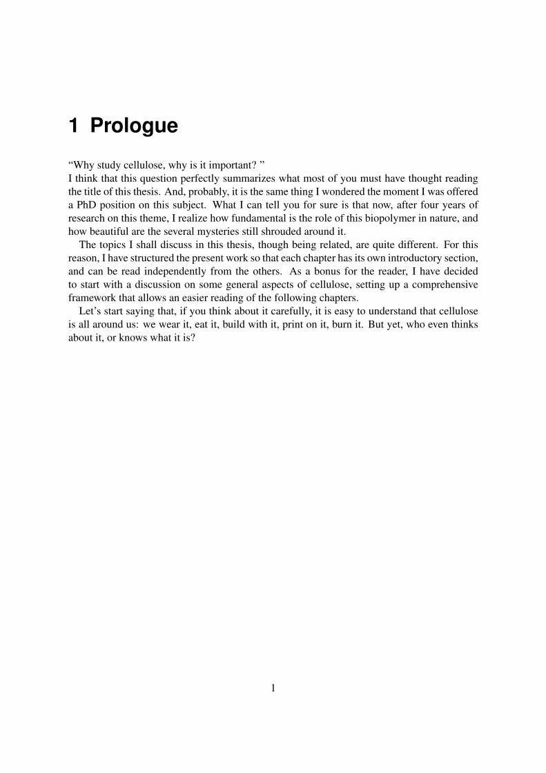
Chemically, cellulose appears simple: it is a linear polymer of β-(1,4) glucose, where everytwo adjacent glucose molecules are linked together in opposite orientations (Fig. 2.1a). Cel-lobiose, which consists of a pair of glucose residues rotated of 180 with respect to each other,is thus the repeating structural unit of cellulose. The linkage pattern and the flat conformationof the glucan rings confer a ribbon-like shape and semi-rigid properties to the polymer, andthis particular molecular structure enables the cellulose molecules to crystallize into rigid rodscalled microfibrils (CMFs) (Fig. 2.1b). This crystalline, microfibrillar form, allows celluloseto play its structural role in nature.
Figure 2.1: a) Chemical structure of a single cellulose chain. b) Crystalline cellulose microfib-ril (CMF)
Most of the cellulose is made by vascular plants, but its synthesis also occurs in the algae, inthe slime mold Dictyostelium, in a number of bacterial species, and in tunicates in the animalkingdom. Photosynthetic microbes, the first in the vast food chain, also represent an importantresource for cellulose production in nature: without these organisms all animal life in the
3

2 Introduction
oceans would cease to exist. Land plants assemble cellulose from glucose, which is created inthe living plant cell through photosynthesis. In the oceans, most of the cellulose is producedby unicellular plankton or algae using the same type of carbon dioxide fixation found in thephotosynthesis of vascular plants.
2.2 Different types of cellulose
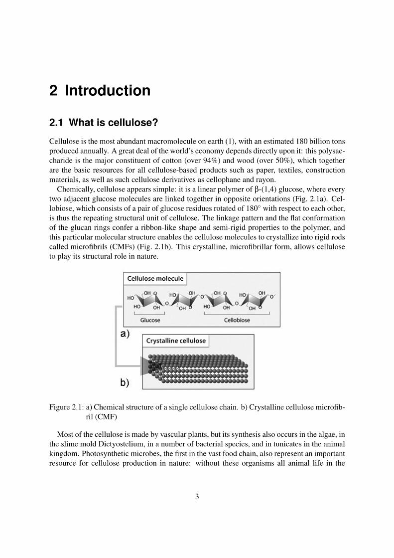
Cellulose is a remarkable structure, and depending on the sources from which it is obtained, itsphysical properties, such as the degree of crystallinity and the molecular weight, may be highlyvariable. There are crystalline and noncrystalline forms of cellulose: the first one is character-ized by a tensile strength greater than steel, and it can be found as cellulose I or cellulose II(Fig. 2.2). Both of these two allomorphs can be directly synthesized in nature; however, cellu-lose I is by far the most prevalent, and no eukaryotic cells are known to abundantly synthesizecellulose II in vivo. Surprisingly, the cellulose I allomorph is a thermodynamically metastableform (2), and can be converted directly to cellulose II with treatment of a high concentrationof sodium hydroxide (NaOH), a process called mercerization; however, cellulose II cannot bedirectly converted to cellulose I.
• Cellulose IIn nature, and in most of all plants, cellulose is generally produced as crystalline cellu-lose I (Fig. 2.2a/c and Fig. 2.3b), in which the glucan chains are parallel to each other(3; 4) and are packed side by side to form CMFs that are typically 3nm thick, but whichcan reach widths of 60nm in certain algae. There are two known suballomorphs ofcellulose I: Ia and Ib (5; 6). These two forms differ with respect to their molecularconformation, hydrogen bonding and crystal packing, but can usually coexist togetherwithin a given CMF, whose physical properties will be dependent on the ratio of thesetwo suballomorphs. Cellulose from some algae and bacteria is found to be Ia rich, whilecellulose from cotton wood is Ib rich (7). The tunicates, the only animal to producecellulose (8), appear to synthesize almost exclusively cellulose Ib.
• Cellulose IIA few organisms produce crystalline cellulose II (Fig. 2.2b/d) naturally. This form isgenerally synthesized by mutants of Acetobacter Xylinum (9), a bacterium that normallyproduces cellulose I. The glucan chains arrangement in cellulose II has been proposedto be antiparallel (Fig. 2.3c), and this disposition may take place as a result of chainfolding during synthesis (9). An additional hydrogen bond per glucan chain residue incellulose II makes this allomorph be the most thermodynamically stable form. CelluloseI which has undergone mercerization is cellulose II: however, chain folding has not beendemonstrated in this type of cellulose II. Understanding the structure of cellulose IIderived from mercerized products is one of the remaining issue about cellulose structureto be elucidated.
• Non-crystalline celluloseApart from the crystalline states, cellulose also occurs in non-crystalline states, and
4
2 Introduction
this form has been observed to be present along with the cellulose I crystallites in someCMFs. A new form of derived cellulose, referred to as nematic ordered cellulose (NOC),is obtained by dissolving native cellulose and reprecipitating it in a unique manner toform a distinctive structure (10) highly ordered yet not crystalline: films obtained fromthis type of cellulose exhibit properties different from conventional cellulose films. Inthe majority of cases, cellulose modified after synthesis has properties not found in thenative cellulose that is obtained from living organisms.
Figure 2.2: Images of (a) cellulose I and (b) cellulose II specimen. Projections of the 3d struc-ture of (c) cellulose Ib and (d) cellulose II
2.3 Biogenesis of Cellulose I
As mentioned in the previous section, the most common natural allomorph of cellulose iscellulose I. Since in this thesis we will be mostly concerned with this type of cellulose, in thefollowing we recall the basic concepts related to the biogenesis of this polymer.
Cellulose I consists of crystalline CMFs in which the glucan chains are parallel and ex-tended. The substrate for cellulose synthesis is UDP-glucose, which is channeled through thecellulose synthase complex (CSC) and transformed into linear chains of glucose residues (seeChapter 4 for details). The CSCs are multiparticulate enzymes, that are usually found in the
5
2 Introduction
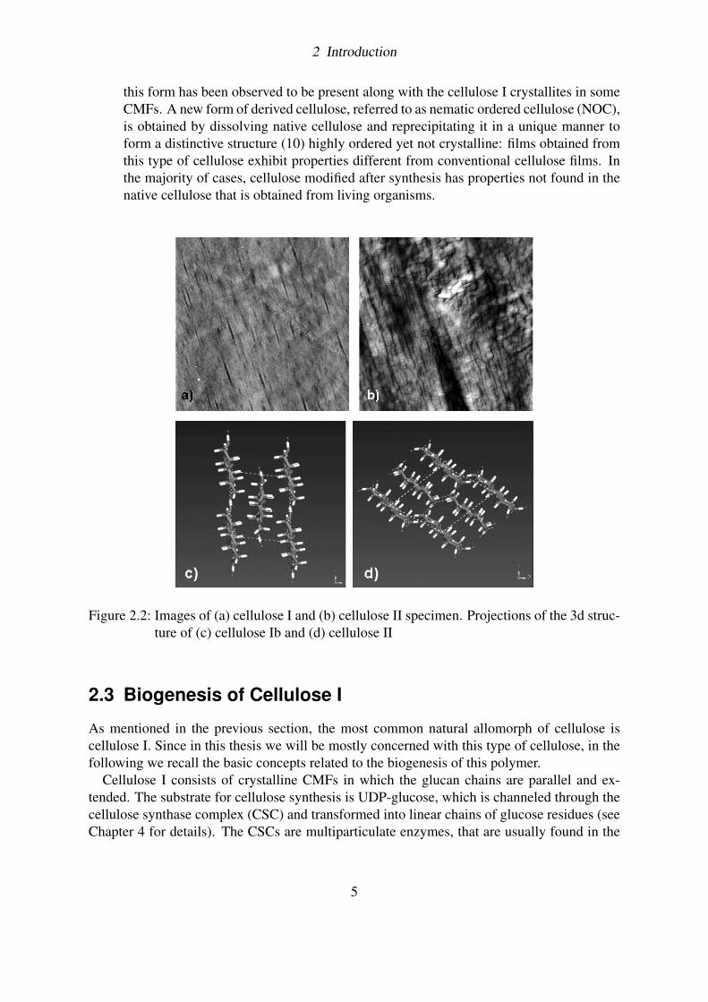
membranes of cells (plants, algae and bacteria), and which contain a number of catalytic siteseach putatively polymerizing a single glucan chain. Surveying all the different type of existingCSCs in nature (see Chapter 3 for details), it is believed that the mechanism of polymerizationis conserved in all these enzymes: cellulose is synthesized processively, with the growing endof the glucan chain (the non-reducing end) tightly associated with the catalytic region of theCSC.
Figure 2.3: b) Parallel and c) antiparallel arrangement of a) cellulose chains
This description indicates that there are two main levels of organization of cellulose (11):first, glucose molecules have to be synthesized and linked into a long chain (polymerization);second, many cellulose polymers coalesce together to form the CMF (crystallization). Thesize, shape and degree of crystalline perfection is largely due to the geometrical positioningof the catalytic sites within the enzyme complex (see Chapter 3 and Chapter 4 for details).Because of these hierarchical levels of cellulose organization, it is most appropriate to refer tocellulose biogenesis rather than simply biosynthesis.
2.3.1 Polymerization and Crystallization
Recently, a lot of work has been done in order to produce the in vitro synthesis of celluloseI. One of the reasons that have made these experiments so intriguing and so difficult, is thatcellulose I is only a metastable state (2): thus, in vitro systems must be mimicking in some waythe conditions favoured not only for β-(1,4) linked polymerization, but also for crystallizationinto a less stable state. Cellulose biogenesis is a hierarchical process, with polymerizationand crystallization being two distinct, but not completely separated, events (11), linked insuch a way to influence each other: the parallel arrangement of the glucan chains in the CMFrequires in fact the newly synthesized polymers to align with each other and lock into a specificcrystal structure (cellulose I), otherwise they would fold into the more thermodynamicallystable cellulose II, or simply exist as non-crystalline cellulose. The coordinated synthesis of alarge number of glucan chains from ordered sites present in the CSC, allows these polymersto be positioned adjacent to each other before they crystallize.
The main proof that polymerization and crystallization are coupled processes in cellulosebiogenesis comes from studies on Acetobacter Xylinum: in this cellulose producing bac-
6
2 Introduction
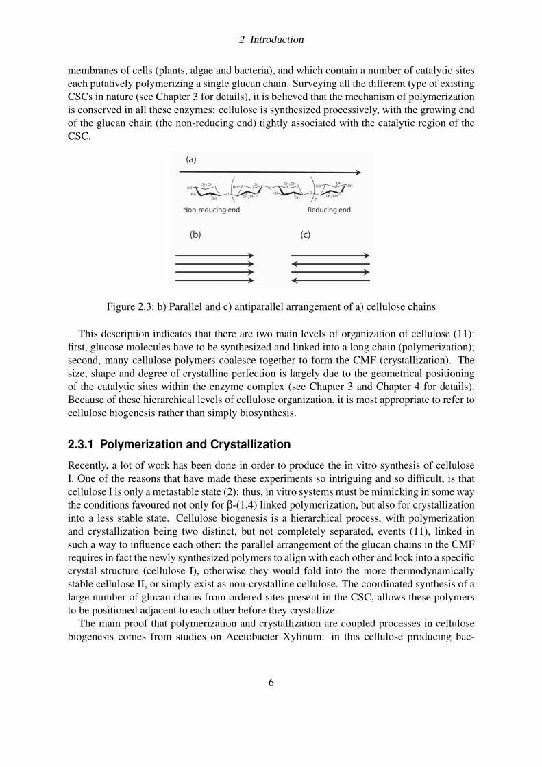
terium, it has been seen that an optical brightener, Calcofluor White ST (11), inhibits thecrystallization preventing the formation of the cellulose CMFs. Interestingly enough, this re-sults in an increase in the rate of cellulose polymerization by an amount that varies between 2and 4 times the control rate. This could indicate that the time required for the glucan chainsto crystallize limits the rate at which polymerization proceeds. In any case, it demonstrates aclear inter-dependence between these two processes.
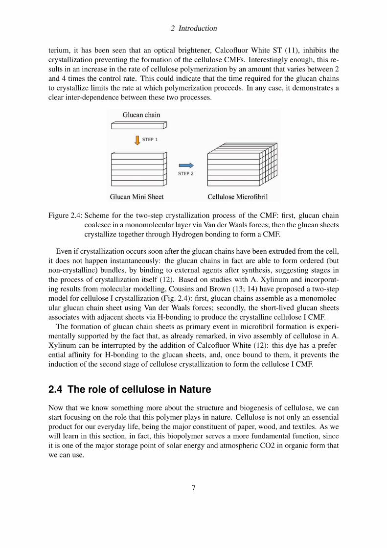
Figure 2.4: Scheme for the two-step crystallization process of the CMF: first, glucan chaincoalesce in a monomolecular layer via Van der Waals forces; then the glucan sheetscrystallize together through Hydrogen bonding to form a CMF.
Even if crystallization occurs soon after the glucan chains have been extruded from the cell,it does not happen instantaneously: the glucan chains in fact are able to form ordered (butnon-crystalline) bundles, by binding to external agents after synthesis, suggesting stages inthe process of crystallization itself (12). Based on studies with A. Xylinum and incorporat-ing results from molecular modelling, Cousins and Brown (13; 14) have proposed a two-stepmodel for cellulose I crystallization (Fig. 2.4): first, glucan chains assemble as a monomolec-ular glucan chain sheet using Van der Waals forces; secondly, the short-lived glucan sheetsassociates with adjacent sheets via H-bonding to produce the crystalline cellulose I CMF.
The formation of glucan chain sheets as primary event in microfibril formation is experi-mentally supported by the fact that, as already remarked, in vivo assembly of cellulose in A.Xylinum can be interrupted by the addition of Calcofluor White (12): this dye has a prefer-ential affinity for H-bonding to the glucan sheets, and, once bound to them, it prevents theinduction of the second stage of cellulose crystallization to form the cellulose I CMF.
2.4 The role of cellulose in Nature
Now that we know something more about the structure and biogenesis of cellulose, we canstart focusing on the role that this polymer plays in nature. Cellulose is not only an essentialproduct for our everyday life, being the major constituent of paper, wood, and textiles. As wewill learn in this section, in fact, this biopolymer serves a more fundamental function, sinceit is one of the major storage point of solar energy and atmospheric CO2 in organic form thatwe can use.
7
2 Introduction
Let’s start from the beginning: as previously said in this chapter, cellulose is made up ofglucose, which is a primary product of photosynthesis. This process, that can be illustrated asfollows
6H2O+6CO2 + light energy−→ C6H12O6 +6O2
essentially converts light energy in chemical energy, producing a molecule of glucose plus sixof oxygen starting from water, carbon dioxide (CO2), and light. Through the process of photo-synthesis, green plants absorb solar energy and remove CO2 from the atmosphere to producesugars. Plants and animals burn these carbohydrates (and other products derived from them)through respiration, the reverse of photosynthesis, a process that releases the energy containedin sugars for use in metabolism, and renders the carbohydrate fuel back to carbon dioxide.Together, respiration and decomposition (respiration that consumes organic matter mostly bybacteria and fungi) return the biologically fixed carbon back to the atmosphere. This vast in-terplay between the CO2 of the atmosphere and its "fixation" via photosynthesis into organicproducts, among which cellulose is the most abundant, is called “carbon cycle”(Fig. 2.5).
In addition to the natural fluxes of carbon through the Earth system, human activities, par-ticularly fossil fuel burning and deforestation, are also releasing carbon dioxide into the atmo-sphere. When we mine coal and extract oil from the Earth’s crust, and then burn these fossilfuels for transportation, heating, cooking, electricity, and manufacturing, we are effectivelymoving carbon more rapidly into the atmosphere than is being removed naturally throughthe sedimentation of carbon, ultimately causing the concentration of atmospheric CO2 to in-crease. Moreover, by clearing forests to support agriculture, we are transferring carbon fromliving biomass into the atmosphere (dry wood is about 50 percent carbon). The result is thathumans are adding ever-increasing amounts of extra carbon dioxide into the atmosphere. Be-cause of this, atmospheric CO2 concentrations are higher today than they have been over thelast half-million years or longer. This emerging problem could have immense consequencesif the CO2 content continues to rise: the global warming cycle, affected by the emergence ofthe industrial age, is in fact closely related to this issue.
In this context, the role of cellulose within the global carbon cycle is fundamental: cellulosecan be thought of as a giant carbon "sink" that fixes the atmospheric CO2 in organic form.Most of the organic compounds that are formed as a result of CO2 fixation in the bodies ofphotosynthetic organisms are ultimately broken down and released back into the atmosphereor water. However, certain carbon-containing compounds, such as cellulose, are more resistantto breakdown than others, and carbon incorporation into cellulose remains in the product fora rather lengthy time, sometimes for thousands of years. This makes clear the importance thatthis biopolymer has not only in our everyday’s life, but also, and most of all, on large timescale events, through the balancing of CO2 levels over long time periods.
A possible solution to the extra CO2 amounts in the atmosphere would be to reverse theconversion process by increasing photosynthesis, which results in the trapping of more carbondioxide. It is straightforward to understand that a good way to accomplish this task is toenhance the production of cellulose, developing organisms that are able to synthesize thispolymer more efficiently and in improved forms. It is also clear that in order to do that, weneed to know more about the mechanisms that control and regulate cellulose production indifferent organisms.
8

2 Introduction
Figure 2.5: The carbon Cycle on earth: the numbers show the total amount of stored carbon(black) and the annual carbon fluxes (gray)
2.5 This Thesis
In this context this thesis can be thought of as an attempt to gather together and elucidatea number of open biological problems concerning the synthesis, crystallization and self-organization of cellulose. Using theoretical methods coupled to simulation techniques, weanalyze the mechanism at the basis of cellulose biosynthesis by focusing on two of the mostimportant cellulose producing entities: plant cells and Acetobacter bacteria. The first threechapters of this thesis (3-5) will be therefore related to different issues concerning cellulosebiosynthesis in plant cells, while the last chapter will deal with cellulose production in Aceto-bacter cells.
We start in Chapter 3 proposing a mechanism for the the self-assembly of the cellulosesynthase complex (CSC) in higher plants. At present, rather little is know about the internalstructure of this protein, as well as about the molecular mechanism that regulates its forma-tion. This enzyme, named also hexagonal rosette, is a transmembrane complex thought to becomposed of 36 subunits, the CESA proteins. Using experimental evidences and results frommutants analysis, it is possible to obtain information on the mutual and specific interactionsbetween the CESA. The knowledge of this interaction scheme allows the formulation of adynamical model, which we will subsequently implement in a MonteCarlo simulation, that isable to reproduce the processive assembly of the final hexagonal complex.
After having studied the formation of the CSC, we pursue presenting a biophysical modelthat explains the force generating mechanism underlying the propulsion of this enzyme. Whilepolymerizing the cellulose microfibrils (CMFs), the CSC walks through the plasma membraneof plant cells. Early theories assumed the CSC to be linked by motor proteins to the cortical
9
2 Introduction
microtubules, supposed to act as rails to guide its motion. In Chapter 4 we present an alter-native model for the propulsion of the CSC: we show how the growth of the cellulose CMFsagainst the membrane causes an accumulation of elastic energy: the energy release, controlledby thermal fluctuations, happens in the form of unidirectional force and propels the CSCthrough the membrane. Our model is able to provide an estimate for the velocity of the CSCas a function of the other relevant parameters of the system (bending energies, temperatureand polymerization rate constants) that is very close to the experimental value.
We go on investigating in Chapter 5 the process involved in cell wall deposition: dependingon the orientation of the CMFs in the plant cell wall, one can obtain very regular and differenttextures, among which the helicoidal pattern is the most striking one. A fundamental andfascinating question is how the CMFs become oriented during the deposition at the plasmamembrane. The current textbook explanation for this phenomenon is again a guidance systemmediated by cortical microtubules. However, too many contradictions are known for this tobe a universal mechanism, notably in the case of helicoidal arrangements, which occur inmany situations. Our aim in this Chapter is to use geometrical considerations to formulate amathematical model for the spatio-temporal evolution of the orientation of the CMFs in thecell wall. We show how the solutions of our model can generate a great variety of textures,including the helicoidal one. Moreover, we show that our solutions are robust against differentperturbations and noise effects, suggesting that this mechanism can be considered a strong andsuccessful tool for the explanation of a great variety of cell wall textures.
Finally, in Chapter 6, we focus our attention on Acetobacter bacteria. These rod-shapedorganisms live at the air-liquid interface and swim while producing a long and flat celluloseribbon. The ribbon is composed by cellulose CMFs that are synthesized by a row of catalyticsites positioned along the long axis of the cell. Once polymerized, the CMFs cooperativelybend and become oriented along the axis of the bacterium. The aim of this Chapter is toexplain such orientation mechanism, by the means of theoretical and numerical techniques.Our goal is to correlate this phenomenon with a hydrodynamic effect due to the interactionsbetween the cellulose chains and the fluid in which they are immersed. To demonstrate thatthis can actually be the case, in the second part of the Chapter we implement a Brownian Dy-namics simulation which explicitly reproduces the bacterial motion together with the celluloseorientation mechanism.
With this work we hope to contribute in elucidating some key questions, both regarding thecell biology of plants as well as concerning the physics of interacting filaments and complexmacromolecular assemblies.
10
3 The Cellulose Synthase Complex
The universal distribution of cellulose among prokaryotic and eukaryotic organisms attests toits ancient evolutionary history. This polysaccharide is in fact synthesized by all land plants, anumber of bacterial species, many groups of algae, the slime mold Dictyostelium and tunicatesin the animal kingdom. It is an extracellular polymer, and with the exception of bacteria andtunicates, it is generally the main component of the cell-wall, a rigid shell that surrounds thecell. The diverse function that cellulose plays in different groups of organisms is reflected bythe particular structure of the polymerizing enzyme, the cellulose synthase complex (CSC), ineach of the different species. Even though specific features are found in CSCs from differentorganisms, it is believed that the catalytic region is conserved in all these enzymes.
The goal of this chapter is to provide a comprehensive view of the structure and the featuresof the CSC in different organisms. To do this, we first illustrate examples of CSCs in variousspecies. Then we narrow our attention to plants, analyzing in detail the structure and thechemical composition of the CSC in this case. Finally, we build a model that elucidatesthe assembly of this enzyme in plants, algae and bacteria, and which suggests how a uniquemechanism may be responsible for the formation of this multiform protein complex at least inthese three species.
3.1 A bit of history...
One of the great enigmas in plant biology is the biosynthesis of cellulose. During the past50 years, the site of cellulose synthesis has been investigated intensively, but until few yearsago there had been no direct proof for the presence of the multimeric enzyme complex whoseexistence had been postulated by Preston in 1964 (15). According to Preston’s theory, the“Ordered Granule Hypothesis”, an array of catalytic subunits forming the cellulose synthase,would function together to synthesize glucan chains that would then self-assemble to form acellulose microfibril (CMF). In the 1960s, with the advent of the freeze fracture technique, ca-pable of revealing replicas of the interior of membrane surfaces, investigators began to noticehighly ordered, multiparticulate protein subunits in association with cell membranes. In 1976Preston’s vision was realized as being most likely true with the first successful application offreeze fracture on the membrane of the fresh water alga “Oocystis apiculata” (Fig. 3.1a) thatled to the imaging of ordered structures at the tip of the CMFs.
These structures were linear multimeric arrays, termed “linear terminal complexes” (linearTCs), and consisted of three rows of subunit particles. The complexes were intimately as-sociated with the CMFs, as clearly evidenced by impressions of the cellulose fibrils on theE-fracture face of the plasma membrane. Subsequently, in 1980, a different arrangement wasfound for the cellulose enzyme (16), a cluster of six particles associated with CMF’s imprints
11
3 The Cellulose Synthase Complex
in the P-fracture face of the plasma membrane of corn root cells (Fig. 3.1b). Due to the regularhexagonal arrangement of its six transmembrane subunits these particles were named “rosetteTCs”. Although already identified for several decades, the definite biochemical proof thatthese structures indeed are the location of the cellulose synthases in vascular plants, was onlyprovided in 1999 (17). Eventually the rosettes have been found to be exclusive for all landplant cellulose assembly, including mosses, ferns, liveworts and certain green alga.
In the following we will use for the cellulose TCs (linear or rosette) the most general nomen-clature “cellulose synthase complex” (CSC).
3.2 The diversity of CSCs: shape and arrangement
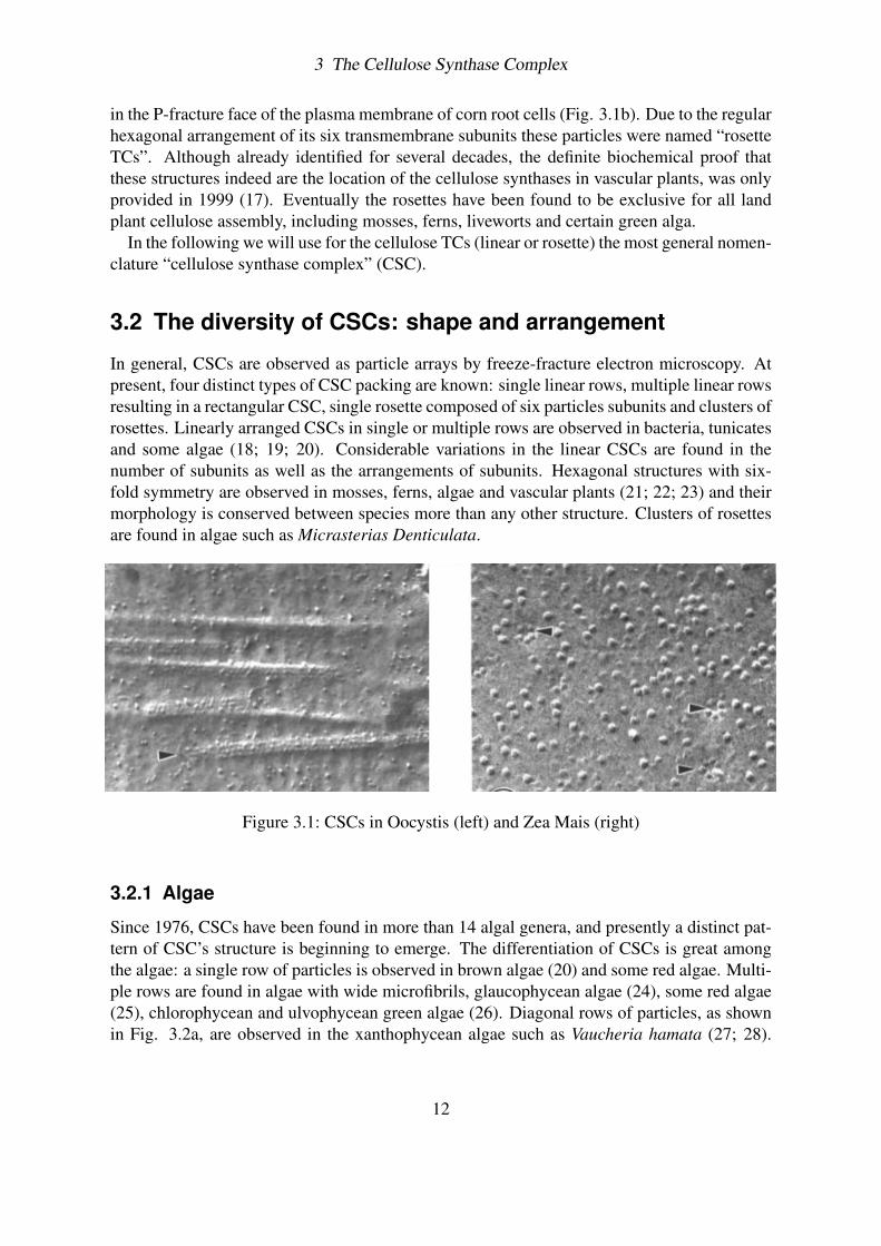
In general, CSCs are observed as particle arrays by freeze-fracture electron microscopy. Atpresent, four distinct types of CSC packing are known: single linear rows, multiple linear rowsresulting in a rectangular CSC, single rosette composed of six particles subunits and clusters ofrosettes. Linearly arranged CSCs in single or multiple rows are observed in bacteria, tunicatesand some algae (18; 19; 20). Considerable variations in the linear CSCs are found in thenumber of subunits as well as the arrangements of subunits. Hexagonal structures with six-fold symmetry are observed in mosses, ferns, algae and vascular plants (21; 22; 23) and theirmorphology is conserved between species more than any other structure. Clusters of rosettesare found in algae such as Micrasterias Denticulata.
Figure 3.1: CSCs in Oocystis (left) and Zea Mais (right)
3.2.1 Algae
Since 1976, CSCs have been found in more than 14 algal genera, and presently a distinct pat-tern of CSC’s structure is beginning to emerge. The differentiation of CSCs is great amongthe algae: a single row of particles is observed in brown algae (20) and some red algae. Multi-ple rows are found in algae with wide microfibrils, glaucophycean algae (24), some red algae(25), chlorophycean and ulvophycean green algae (26). Diagonal rows of particles, as shownin Fig. 3.2a, are observed in the xanthophycean algae such as Vaucheria hamata (27; 28).
12

3 The Cellulose Synthase Complex
In contrast to linear CSCs, some species of algae show rosette CSCs which appear identicalto those in vascular plants. All embryophytes, the Zygnematales, the Coleochateles and theCharales, which are thought to be the closest relatives of land plants, (23) have six particlesrosette, except for Coleochaete Scutata, which has a unique CSC consisting of eight particles.Differently from any other alga, the Micrasterias Denticulata shows the typical rosette CSConly during primary wall synthesis. During secondary wall synthesis in fact the single rosettesaggregate forming hexagonally ordered complexes (Fig. 3.2b) that result in synthesis of bandsof thicker microfibrils (29).
Figure 3.2: CSCs in Vaucheria (left) and Micrasterias Denticulata (right)
3.2.2 Bacteria
Among the prokaryotes, the purple bacteria are thought to be the most advanced (30), beingconsidered as progenitors of mitochondria in the eukaryotic cell (31). Interestingly, manygenera in this group synthesize cellulose. The best known examples are various species ofAcetobacter, Rhizobium and Agrobacterium (32; 33). Among these, Acetobacter Xylinum isa model system for the understanding of cellulose biosynthesis from the aspects of moleculargenetics and biochemistry: it produces massive amounts of cellulose, which is secreted not asa cell wall polymer like in eukaryotes, but as an extracellular pellicle (for more informationon Acetobacter Xylinum go to Chapter 6). In all purple bacteria the site of cellulose synthesisis a linear row of particles parallel to the longitudinal axis of the cell (18).
In addition to this bacterial group, also Escherichia Coli, Klebsiella Pneumoniae, Salmonella(34) and Sarcina Ventriculi (35) produce cellulose.
13
3 The Cellulose Synthase Complex
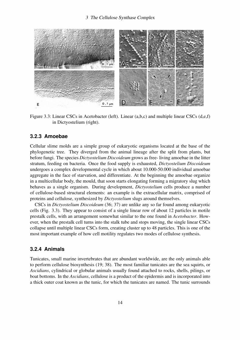
Figure 3.3: Linear CSCs in Acetobacter (left). Linear (a,b,c) and multiple linear CSCs (d,e,f)in Dictyostelium (right).
3.2.3 Amoebae
Cellular slime molds are a simple group of eukaryotic organisms located at the base of thephylogenetic tree. They diverged from the animal lineage after the split from plants, butbefore fungi. The species Dictyostelium Discoideum grows as free- living amoebae in the litterstratum, feeding on bacteria. Once the food supply is exhausted, Dictyostelium Discoideumundergoes a complex developmental cycle in which about 10.000-50.000 individual amoebaeaggregate in the face of starvation, and differentiate. At the beginning the amoebae organizein a multicellular body, the mould, that soon starts elongating forming a migratory slug whichbehaves as a single organism. During development, Dictyostelium cells produce a numberof cellulose-based structural elements: an example is the extracellular matrix, comprised ofproteins and cellulose, synthesized by Dictyostelium slugs around themselves.
CSCs in Dictyostelium Discoideum (36; 37) are unlike any so far found among eukaryoticcells (Fig. 3.3). They appear to consist of a single linear row of about 12 particles in motileprestalk cells, with an arrangement somewhat similar to the one found in Acetobacter. How-ever, when the prestalk cell turns into the stalk tube and stops moving, the single linear CSCscollapse until multiple linear CSCs form, creating cluster up to 48 particles. This is one of themost important example of how cell motility regulates two modes of cellulose synthesis.
3.2.4 Animals
Tunicates, small marine invertebrates that are abundant worldwide, are the only animals ableto perform cellulose biosynthesis (19; 38). The most familiar tunicates are the sea squirts, orAscidians, cylindrical or globular animals usually found attached to rocks, shells, pilings, orboat bottoms. In the Ascidians, cellulose is a product of the epidermis and is incorporated intoa thick outer coat known as the tunic, for which the tunicates are named. The tunic surrounds
14

3 The Cellulose Synthase Complex
the surface of the animal’s soft body to protect it against predators, it is often transparent ortranslucent and varies in consistency from gelatinous to leathery. The structure of CSCs inTunicates was categorized at first to the linear type (21). However, the CSCs of most of theAscidians have a unique feature as compared with other types of linear CSCs that have beenfound in bacteria, algae and slime molds. They are composed of two kinds of membraneparticles (Fig. 3.4): small subunits (7.2 nm) corresponding to the cellulose synthases, andlarge particles (14.5 nm in diameter) surrounding the synthase complexes. It is not clear,however, whether this feature of “double CSCs” is universal in all Ascidians or not.
Figure 3.4: CSCs in Tunicates
3.3 Cellulose CSCs in higher plants
Interestingly, among the vascular plants only the rosette CSC (Fig. 3.5) has been found.Thus, algal ancestors with rosette CSCs have assumed additional importance with respectto understanding the evolution of land plants. The rosette CSC was first described by Mullerand Brown in 1980 in Zea mays (16). In vascular plants, like mosses and ferns, gymnospermsand angiosperms (39), this enzyme appears as a protein complex with a six-fold symmetry anda diameter of 25nm.
The genes that encode the catalytic subunits of cellulose synthase are called CESA genes.They were first identified at the molecular level in the cellulose producing bacteria Acetobacterand Agrobacterium (review in (22)). From the sequences of these enzymes, motifs character-istic of cellulose synthase have subsequently been recognized. In the late 1990 the first CESAsof a plant were identified trough molecular and genetic studies (40; 41). Presently the mostinformation is known about the Arabidopsis Thaliana CESA gene family, the AtCESA, sincethe Arabidopsis genome is fully sequenced. In this model plant the CESA family contains atleast ten genes, which are expressed in different tissues and cell types. Sequence data indicatethat the CESA gene family is as large, or larger, in other plants species.
15
3 The Cellulose Synthase Complex
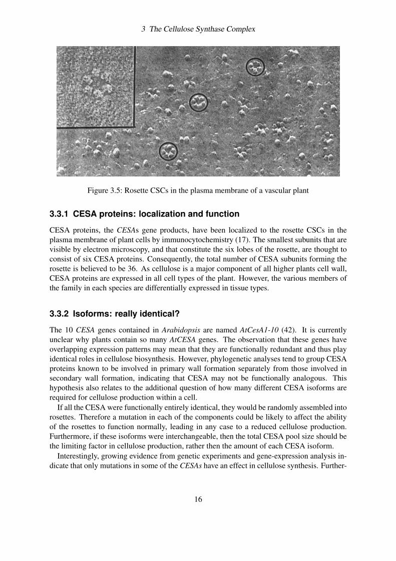
Figure 3.5: Rosette CSCs in the plasma membrane of a vascular plant
3.3.1 CESA proteins: localization and function
CESA proteins, the CESAs gene products, have been localized to the rosette CSCs in theplasma membrane of plant cells by immunocytochemistry (17). The smallest subunits that arevisible by electron microscopy, and that constitute the six lobes of the rosette, are thought toconsist of six CESA proteins. Consequently, the total number of CESA subunits forming therosette is believed to be 36. As cellulose is a major component of all higher plants cell wall,CESA proteins are expressed in all cell types of the plant. However, the various members ofthe family in each species are differentially expressed in tissue types.
3.3.2 Isoforms: really identical?
The 10 CESA genes contained in Arabidopsis are named AtCesA1-10 (42). It is currentlyunclear why plants contain so many AtCESA genes. The observation that these genes haveoverlapping expression patterns may mean that they are functionally redundant and thus playidentical roles in cellulose biosynthesis. However, phylogenetic analyses tend to group CESAproteins known to be involved in primary wall formation separately from those involved insecondary wall formation, indicating that CESA may not be functionally analogous. Thishypothesis also relates to the additional question of how many different CESA isoforms arerequired for cellulose production within a cell.
If all the CESA were functionally entirely identical, they would be randomly assembled intorosettes. Therefore a mutation in each of the components could be likely to affect the abilityof the rosettes to function normally, leading in any case to a reduced cellulose production.Furthermore, if these isoforms were interchangeable, then the total CESA pool size should bethe limiting factor in cellulose production, rather then the amount of each CESA isoform.
Interestingly, growing evidence from genetic experiments and gene-expression analysis in-dicate that only mutations in some of the CESAs have an effect in cellulose synthesis. Further-
16
3 The Cellulose Synthase Complex
more, it has been shown that in some cases one CESA isoform cannot effectively compensatefor the loss of another. This strongly suggests that the presence of some of the isoforms is crit-ical for cellulose synthesis, and argues a case for non-random incorporation of CESA proteinsinto rosettes.
3.3.3 Mutants
There are a number of mutants currently known in plant cellulose synthase genes. Here we listthe most important mutations in Arabidopsis Thaliana (for simplicity we will omit the gene’sprefix At-).The rsw1 temperature-sensitive mutation in CESA1, when grown at the non-permissive tem-perature, causes a specific reduction in cellulose synthesis in primary cell wall, the accumu-lation of non-crystalline β(1,4) glucan, disassembly of cellulose synthase, and widespreadmorphological abnormalities (41).In addition to rsw1, mutations in CESA6 gene results in a deficiency in cellulose in primarycell wall. This suggest that both CESA1 and CESA6 are required for cellulose synthesis in theprimary cell wall.The irx3 (irregular xylem3) point mutation in CESA7 shows a defect in secondary cell wallformation in xylem. As a result, the irx3 mutant have weakened walls and collapse upon them-selves (43; 44). The irx1 point mutation in CESA8 is a member of the same family of mutantsas irx3, and causes a reduced production of cellulose in secondary wall.Not to be confused with irx is ixr1 (isoxaben resistance). There are two mutants alleles, ixr1-1and ixr1-2 that confer resistance to the cellulose biosynthesis inhibitor isoxaben. Both allelesare point mutations in the CESA3 gene, suggesting that this gene may also be required forprimary wall cellulose synthesis. Another mutation that confers resistance to isoxaben is ixr2,a point mutation in the CESA6 gene.Recently a novel mutant, irx5, has been discovered, which has severely reduced secondarycell wall cellulose. This phenotype is caused by a mutation of the CESA4 gene.Finally, procuste1 is one of a class of mutants that show decreased elongation and increasedradial expansion in hypocotyls in Arabidopsis. Procuste1 is mutation a in the CESA6 gene,the same gene as ixr2.
3.4 Rosette structure
The assembly of CESA subunits into hexamers is still not well understood. However, the dataon mutants shown above suggest that there are two different non-overlapping sets, each com-posed at least by three CESA proteins, which are responsible for the formation of an operativecellulose-synthesizing complex. The triplet CESA4, CESA7 and CESA8 (whose mutationcorresponds respectively to the irx5, irx3, and irx1 mutants) is required to correctly assemblethe cellulose rosette in the secondary cell wall (45); on the other hand, CESA1, CESA3 andCESA6 (corresponding to the ixr1, ixr2 and rsw1 mutants) are needed for the synthesis of theprimary wall (41; 46). This hypothesis is consistent with the idea that CESA proteins are notfunctionally redundant but, rather, play distinct roles in the cellulose biosynthesis mechanism.
17
3 The Cellulose Synthase Complex
Understanding how three CESAs interact to form a functional rosette CSC is essential for aproper comprehension of how single β(1,4) chains of glucose are synthesized, and how thesechains become organized into crystalline microfibrils. So far there are two main models pro-posed for the architecture of the rosette: the first one is based on the hypothesized CESAsinteractions in primary cell wall, while the second one makes use of the known experimentalevidences in secondary cell wall extracts.
3.4.1 Model for CESAs interactions in primary cell wall
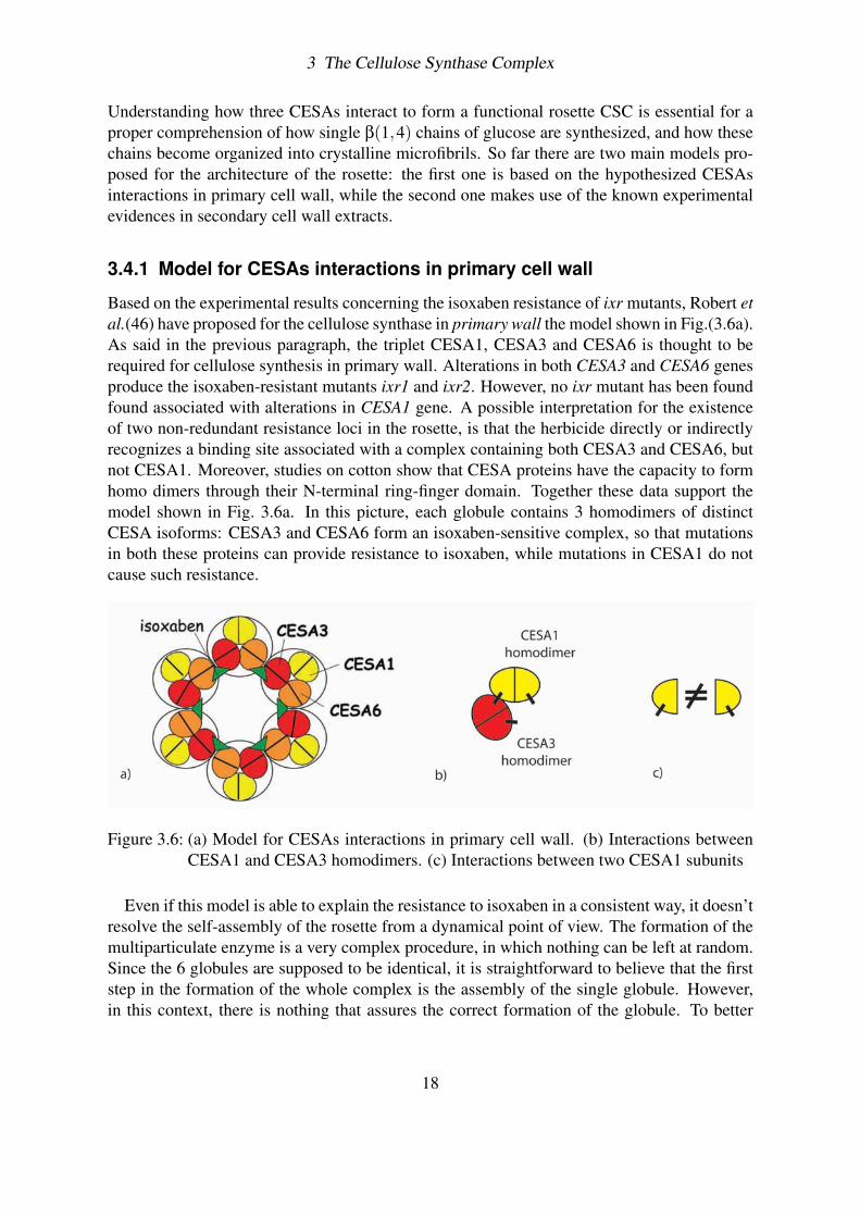
Based on the experimental results concerning the isoxaben resistance of ixr mutants, Robert etal.(46) have proposed for the cellulose synthase in primary wall the model shown in Fig.(3.6a).As said in the previous paragraph, the triplet CESA1, CESA3 and CESA6 is thought to berequired for cellulose synthesis in primary wall. Alterations in both CESA3 and CESA6 genesproduce the isoxaben-resistant mutants ixr1 and ixr2. However, no ixr mutant has been foundfound associated with alterations in CESA1 gene. A possible interpretation for the existenceof two non-redundant resistance loci in the rosette, is that the herbicide directly or indirectlyrecognizes a binding site associated with a complex containing both CESA3 and CESA6, butnot CESA1. Moreover, studies on cotton show that CESA proteins have the capacity to formhomo dimers through their N-terminal ring-finger domain. Together these data support themodel shown in Fig. 3.6a. In this picture, each globule contains 3 homodimers of distinctCESA isoforms: CESA3 and CESA6 form an isoxaben-sensitive complex, so that mutationsin both these proteins can provide resistance to isoxaben, while mutations in CESA1 do notcause such resistance.
Figure 3.6: (a) Model for CESAs interactions in primary cell wall. (b) Interactions betweenCESA1 and CESA3 homodimers. (c) Interactions between two CESA1 subunits
Even if this model is able to explain the resistance to isoxaben in a consistent way, it doesn’tresolve the self-assembly of the rosette from a dynamical point of view. The formation of themultiparticulate enzyme is a very complex procedure, in which nothing can be left at random.Since the 6 globules are supposed to be identical, it is straightforward to believe that the firststep in the formation of the whole complex is the assembly of the single globule. However,in this context, there is nothing that assures the correct formation of the globule. To better
18
3 The Cellulose Synthase Complex
understand this last point, let’s focus on the interactions between the CESA1- and CESA3-homodimers: in order to bind to each other these dimers must share some binding loci, forexample the binding arms shown in Fig. 3.6b. However, for symmetry reason, the proteinsthat form each of the dimers (the two CESA1 and the two CESA3) must be identical to eachother. As you can see form Fig. 3.6c, this is clearly impossible. It is therefore very hardto understand how the three homodimers can interact in the right way to form a functionalglobule, and subsequently a functional rosette.
3.4.2 Model for CESAs interactions in secondary cell wall
The model for the architecture of the rosette in secondary cell wall has been originally pro-posed by Scheible in 2001. In this section we first examine in detail the experimental evidencesthat led to the formulation of this model. Then, based on these results, we build an interactionscheme for the CESAs proteins in secondary cell wall extract. Finally, we implement these in-teractions in a dynamical model, which we demonstrate to be able to reproduce the processiveassembly of the cellulose synthase complex.
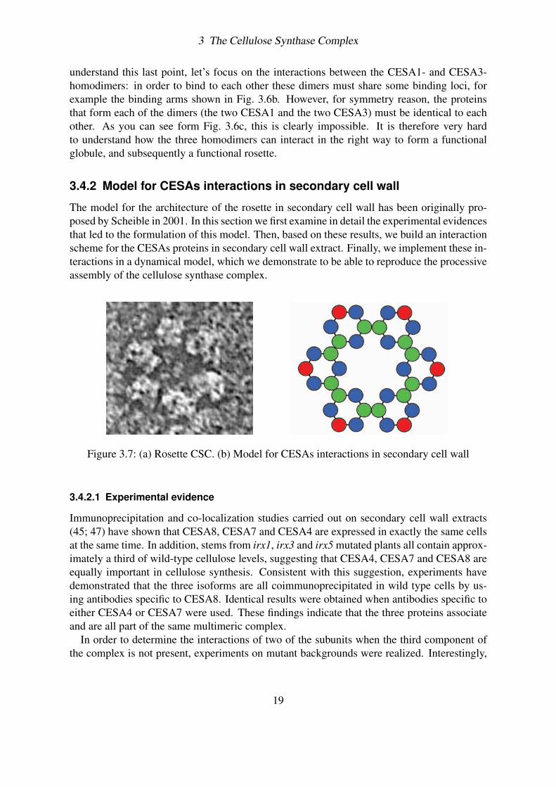
Figure 3.7: (a) Rosette CSC. (b) Model for CESAs interactions in secondary cell wall
3.4.2.1 Experimental evidence
Immunoprecipitation and co-localization studies carried out on secondary cell wall extracts(45; 47) have shown that CESA8, CESA7 and CESA4 are expressed in exactly the same cellsat the same time. In addition, stems from irx1, irx3 and irx5 mutated plants all contain approx-imately a third of wild-type cellulose levels, suggesting that CESA4, CESA7 and CESA8 areequally important in cellulose synthesis. Consistent with this suggestion, experiments havedemonstrated that the three isoforms are all coimmunoprecipitated in wild type cells by us-ing antibodies specific to CESA8. Identical results were obtained when antibodies specific toeither CESA4 or CESA7 were used. These findings indicate that the three proteins associateand are all part of the same multimeric complex.
In order to determine the interactions of two of the subunits when the third component ofthe complex is not present, experiments on mutant backgrounds were realized. Interestingly,
19
3 The Cellulose Synthase Complex
they demonstrate that in solubilized extracts from irx5-1 plants, in which there is no detectableCESA4 protein, CESA8 is no longer precipitated by the anti-CESA7 antibody. At the sametime, in these types of cells, CESA7 is no longer detectable in the proteins precipitated by theanti-CESA8 antibody. To check the validity of the experiment, control tests were conducted:they clearly indicate that CESA8 and CESA7 are both present in the irx5-1 extracts.
Another analysis was performed using a mutated form of CESA8 (in irx1-1 plants). In irx1-1 extracts, antibodies specifically recognizing CESA7 and CESA4 were able to coprecipitateCESA8, in a manner identical to that seen in wild-type. Thus, the presence of a mutated formof CESA8 did not affect the interactions of the three proteins. This suggests that CESA8 maydiffer from CESA4 in that it is not required for assembly of the other two subunits.
3.4.2.2 Rosette self-assembly in secondary wall: the model
If we consider the rosette assembly purely from a theoretical perspective, at least two dif-ferent types of interactions can be envisaged, one between CESA proteins within a rosettesubunit and one between rosette subunits. For symmetry reasons, we consider the six lobesof the rosette being structurally identical. As said before, each of the lobes is thought to becomposed of 6 CESAs, that have to assemble in a highly ordered manner to make a full sizecomplex. Assuming the spatial extent of the three different CESAs to be comparable, weargue an hexagonal arrangement of the six proteins within each rosette subunit.
This disposition implies that the CESAs should have at least two binding sites positionedat 120 one from each other (Fig 3.9). On the other hand, each of the lobes is itself a subunitof the hexagonal rosette, and therefore it also should have two binding sites positioned a 120
one from each other. This is possible only if at least one of the three CESA types possess athird binding sites that links two of the rosette lobes (Fig. 3.8a). Therefore, there must beat least two isoforms, one with 2 binding sites and one with 3 binding sites, for the correctassembly of the rosette to occur. What, then, is the role of the third isoform discussed in theprevious section?
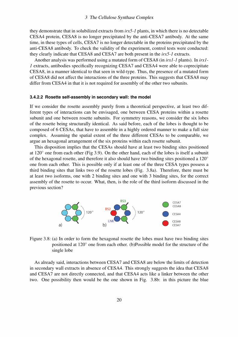
Figure 3.8: (a) In order to form the hexagonal rosette the lobes must have two binding sitespositioned at 120 one from each other. (b)Possible model for the structure of thesingle lobe
As already said, interactions between CESA7 and CESA8 are below the limits of detectionin secondary wall extracts in absence of CESA4. This strongly suggests the idea that CESA8and CESA7 are not directly connected, and that CESA4 acts like a linker between the othertwo. One possibility then would be the one shown in Fig. 3.8b: in this picture the blue
20

3 The Cellulose Synthase Complex
particles, which we will call “linkers” (LNK) from now on, represent the CESA4 proteins; thegreen spheres with three binding sites (BS3) could be exclusively the CESA7 or the CESA8,and the red subunits (BS2) would correspond to the third component of the system. Thisscheme is consistent with the mutant analysis discussed in the last section: in normal cells infact, CESA7 and CESA8 (BS3 and BS2) are linked through CESA4 (LNK) and manage tocoimmunoprecipitate. If LNK is removed, however, like it happens with CESA4 in the irx5-1plant cells, BS2 and BS3 particles are no more connected and behave independently.
Based on these considerations, Doblin proposed for the rosette CSC the structure shown inFig. 3.7b (48; 49). In this model the CESAs are represented as spherical particles that interactwith each other through oriented binding-arms. As illustrated in Fig. 3.9, each of these threeparticle has specific interactions. In particular, LNK can bind with BS3 as well as BS2, BS2can bind only to LNK and BS3 can bind with itself as well as with LNK.
Figure 3.9: Scheme of CESAs interactions
3.5 How does a rosette assemble? Monte Carlo answers...
In order to demonstrate that the interaction scheme displayed in Fig. 3.9 is actually able toresolve the self-assembly of the rosette, we have performed a Monte Carlo simulation. TheMonte Carlo scheme consists of a series of stochastic transitions between different systemconfigurations, all satisfying the imposed constraints. In our simulation each Monte Carlostep involves the displacement (translation or rotation) of a randomly chosen particle. Thesimulation starts with all the particles, of diameter σ, positioned at the vertexes of a grid, ina planar box with reflecting boundary conditions. Since the CESAs particles are thought to
21
3 The Cellulose Synthase Complex
assemble in the plasma membrane, we have performed our simulation in a two-dimensionalspace.
The probability of a given move depends on the energy difference between two successiveconfigurations, i.e. the trial move is accepted with a probability
P(Ei → E f ) = min[1,e−β(E f−Ei)]
where E f and Ei are respectively the energies of the final and initial system state. This rulesatisfies the detailed balance condition that ensures the correct sampling of the equilibriumphase space. After the trial move has been carried out, three situations can occur: 1) theparticle has moved over another particle, in which case the move is rejected because we aresupposing hard-core interactions among the spheres; 2) the particle has moved over a freespot; 3) the particle has bound to another particle.
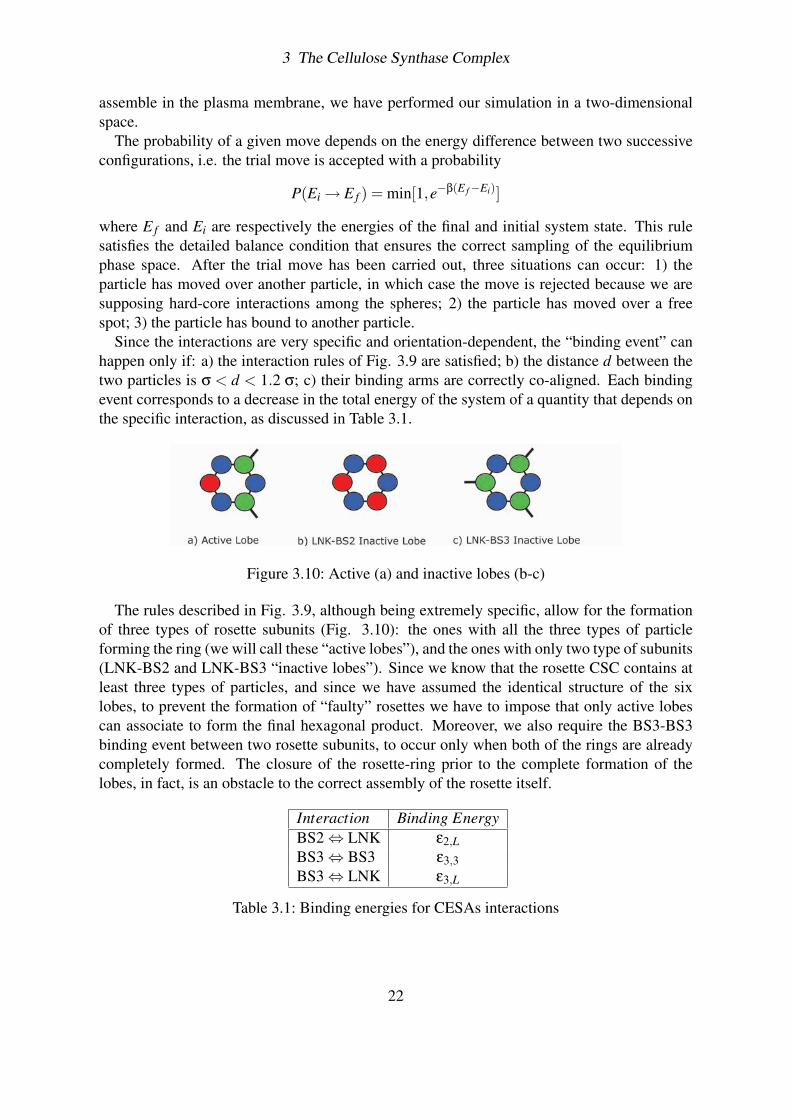
Since the interactions are very specific and orientation-dependent, the “binding event” canhappen only if: a) the interaction rules of Fig. 3.9 are satisfied; b) the distance d between thetwo particles is σ < d < 1.2 σ; c) their binding arms are correctly co-aligned. Each bindingevent corresponds to a decrease in the total energy of the system of a quantity that depends onthe specific interaction, as discussed in Table 3.1.
Figure 3.10: Active (a) and inactive lobes (b-c)
The rules described in Fig. 3.9, although being extremely specific, allow for the formationof three types of rosette subunits (Fig. 3.10): the ones with all the three types of particleforming the ring (we will call these “active lobes”), and the ones with only two type of subunits(LNK-BS2 and LNK-BS3 “inactive lobes”). Since we know that the rosette CSC contains atleast three types of particles, and since we have assumed the identical structure of the sixlobes, to prevent the formation of “faulty” rosettes we have to impose that only active lobescan associate to form the final hexagonal product. Moreover, we also require the BS3-BS3binding event between two rosette subunits, to occur only when both of the rings are alreadycompletely formed. The closure of the rosette-ring prior to the complete formation of thelobes, in fact, is an obstacle to the correct assembly of the rosette itself.
Interaction Binding EnergyBS2 ⇔ LNK ε2,LBS3 ⇔ BS3 ε3,3BS3 ⇔ LNK ε3,L
Table 3.1: Binding energies for CESAs interactions
22
3 The Cellulose Synthase Complex
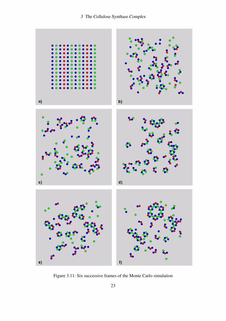
Figure 3.11: Six successive frames of the Monte Carlo simulation
23
3 The Cellulose Synthase Complex
3.5.1 The simulation
Here we present the results of our simulation. The total number of particles in the system is144, and the initial ratio of the three system’s components is exactly the one needed for thecorrect assembly of 4 single rosettes.
Fig. 3.11 shows six snapshots of the simulation. During the first stages of aggregation, theCESAs undergo brownian motion and start to interact forming dimers and trimers of subunits.Subsequently the first rosette subunits begin to emerge (Fig. 3.11b-c), and some of themrapidly aggregate with each other forming two- three-lobes structures (Fig. 3.11d-e). Thesestructures then bind together and the rosette is finally formed (Fig. 3.11f).
Looking carefully at the images we can see that the trimers which are initially formed aremostly LNK-BS2-LNK (blue-red-blue) type. This specific pre-aggregation event is essentialfor the correct formation of active lobes, and strictly depends on the choice of the bindingenergies. By setting conveniently the energies ratios in such a way to have ε2,L >> ε3,L (seeTable 3), it is possible to favour the LNK-BS2-LNK linking with respect to the LNK-BS3-LNK one, and increase in this way its stability. Once these main LNK-BS2-LNK trimersare created, the six lobes can correctly complete their self-assembly. Fig. 3.11b shows somelobes already formed in a pool of subunits. Interestingly, together with correctly assembledlobes, here we can note also the presence of LNK-BS3 inactive complexes, i.e. lobes in whichthe BS2 subunit is missing. Even if the interaction rules of Fig. 3.9 in principle allow forthis anomalous binding to happen, their occurring is rare due to the low stability of thesecomplexes.
3.5.1.1 Need of a chaperone?
For the correct assembly of the rosette to happen we had to make two main assumptions: onlya) active and b) completed lobes can associate to form the hexagon. However, these conditionsare not sufficient to ensure the formation of an intact rosette. The BS3-BS3 binding site in factshould be blocked in some manner for a ring rather than a linear array to be assembled.
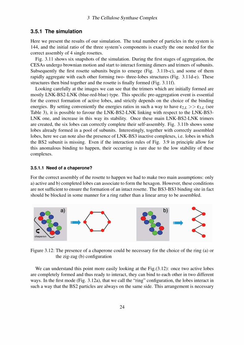
Figure 3.12: The presence of a chaperone could be necessary for the choice of the ring (a) orthe zig-zag (b) configuration
We can understand this point more easily looking at the Fig.(3.12): once two active lobesare completely formed and thus ready to interact, they can bind to each other in two differentways. In the first mode (Fig. 3.12a), that we call the “ring” configuration, the lobes interact insuch a way that the BS2 particles are always on the same side. This arrangement is necessary
24
3 The Cellulose Synthase Complex
for the correct formation of the hexagon ring (Fig. 3.7). In the “zig-zag” configuration thelobes interact in such a way that the red particles are always on opposite sides. Interestingly,this arrangement is not inconsequential, but it brings to the assembly of linear complexes verysimilar in structure at the ones found in some algae and bacteria (Fig. 3.14).
The task of selecting one of the BS3-BS3 binding modes could be performed by chaperones.The chaperone is a molecular complex that aids in the folding of a protein and prevents it fromtaking conformations that would be inactive. In this case one or more chaperones would haveto act like switches, choosing between the linear and the zig-zag configurations depending onthe final CSCs structure that has to form.
3.5.2 What about Micrasterias?
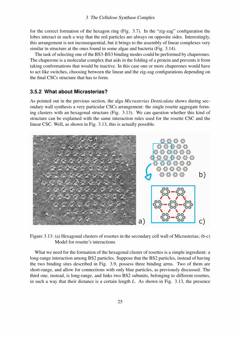
As pointed out in the previous section, the alga Micrasterias Denticulata shows during sec-ondary wall synthesis a very particular CSCs arrangement: the single rosette aggregate form-ing clusters with an hexagonal structure (Fig. 3.13). We can question whether this kind ofstructure can be explained with the same interaction rules used for the rosette CSC and thelinear CSC. Well, as shown in Fig. 3.13, this is actually possible.
Figure 3.13: (a) Hexagonal clusters of rosettes in the secondary cell wall of Micrasterias; (b-c)Model for rosette’s interactions
What we need for the formation of the hexagonal cluster of rosettes is a simple ingredient: along-range interaction among BS2 particles. Suppose that the BS2 particles, instead of havingthe two binding sites described in Fig. 3.9, possess three binding arms. Two of them areshort-range, and allow for connections with only blue particles, as previously discussed. Thethird one, instead, is long-range, and links two BS2 subunits, belonging to different rosettes,in such a way that their distance is a certain length L. As shown in Fig. 3.13, the presence
25
3 The Cellulose Synthase Complex
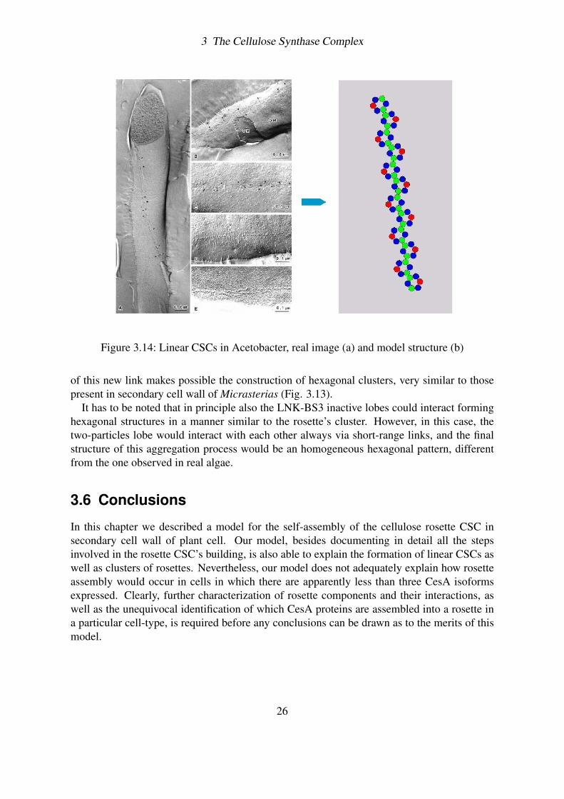
Figure 3.14: Linear CSCs in Acetobacter, real image (a) and model structure (b)
of this new link makes possible the construction of hexagonal clusters, very similar to thosepresent in secondary cell wall of Micrasterias (Fig. 3.13).
It has to be noted that in principle also the LNK-BS3 inactive lobes could interact forminghexagonal structures in a manner similar to the rosette’s cluster. However, in this case, thetwo-particles lobe would interact with each other always via short-range links, and the finalstructure of this aggregation process would be an homogeneous hexagonal pattern, differentfrom the one observed in real algae.
3.6 Conclusions
In this chapter we described a model for the self-assembly of the cellulose rosette CSC insecondary cell wall of plant cell. Our model, besides documenting in detail all the stepsinvolved in the rosette CSC’s building, is also able to explain the formation of linear CSCs aswell as clusters of rosettes. Nevertheless, our model does not adequately explain how rosetteassembly would occur in cells in which there are apparently less than three CesA isoformsexpressed. Clearly, further characterization of rosette components and their interactions, aswell as the unequivocal identification of which CesA proteins are assembled into a rosette ina particular cell-type, is required before any conclusions can be drawn as to the merits of thismodel.
26
4 A polymerization driven molecularmotor
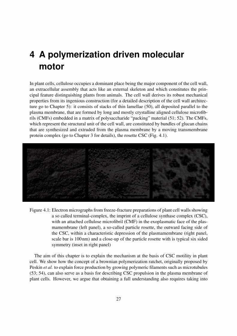
In plant cells, cellulose occupies a dominant place being the major component of the cell wall,an extracellular assembly that acts like an external skeleton and which constitutes the prin-cipal feature distinguishing plants from animals. The cell wall derives its robust mechanicalproperties from its ingenious construction (for a detailed description of the cell wall architec-ture go to Chapter 5): it consists of stacks of thin lamellae (50), all deposited parallel to theplasma membrane, that are formed by long and mostly crystalline aligned cellulose microfib-rils (CMFs) embedded in a matrix of polysaccharide “packing” material (51; 52). The CMFs,which represent the structural unit of the cell wall, are constituted by bundles of glucan chainsthat are synthesized and extruded from the plasma membrane by a moving transmembraneprotein complex (go to Chapter 3 for details), the rosette CSC (Fig. 4.1).
Figure 4.1: Electron micrographs from freeze-fracture preparations of plant cell walls showinga so called terminal-complex, the imprint of a cellulose synthase complex (CSC),with an attached cellulose microfibril (CMF) in the exoplasmatic face of the plas-mamembrane (left panel), a so-called particle rosette, the outward facing side ofthe CSC, within a characteristic depression of the plasmamembrane (right panel,scale bar is 100nm) and a close-up of the particle rosette with is typical six sidedsymmetry (inset in right panel)
The aim of this chapter is to explain the mechanism at the basis of CSC motility in plantcell. We show how the concept of a brownian polymerization ratchet, originally proposed byPeskin et al. to explain force production by growing polymeric filaments such as microtubules(53; 54), can also serve as a basis for describing CSC propulsion in the plasma membrane ofplant cells. However, we argue that obtaining a full understanding also requires taking into
27
4 A polymerization driven molecular motor
account the geometry of the deposition process, the additional driving force provided by thecrystallization of the cellulose, and finally the role of the elastic energy stored in the nascentmicrofibril as well as in the deformable plasma membrane.
4.1 Functioning of the CSC
The assembly of the CSC occurs in the interior of the cell, presumably in the endoplasmicreticulum and in the Golgi apparatus. Current estimates of the diameter of the CSC on the en-doplasmic side are in the range of 40 – 60 nm (55), making the CSC one of the largest proteincomplexes so far observed. Once assembled, the complex is then transported to the plasmamembrane for activation and cellulose synthesis. Since most of the structure of the CSC isdeeply embedded in the cytoplasm of the cell, EM images of freeze fracture preparations ofthe P-face of plant membranes are only able to show a small fraction of the structural unit.What these pictures reveal is a characteristic structure of six hexagonally arranged particlesforming a ring, or “rosette” (56; 16), with diameter of approximately 25 nm (Fig.4.1). At thelocus of the rosette, a depression on the P-side of the membrane (Fig. 4.1b) can be seen toassociate with a bulge on the E-side, from which the growing tip of a CMF departs (Fig. 4.1aand Fig. 4.2a).
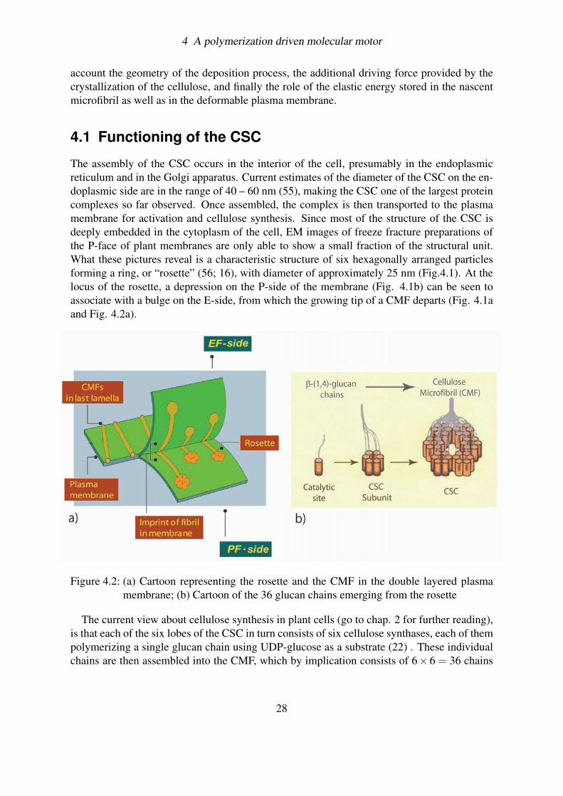
Figure 4.2: (a) Cartoon representing the rosette and the CMF in the double layered plasmamembrane; (b) Cartoon of the 36 glucan chains emerging from the rosette
The current view about cellulose synthesis in plant cells (go to chap. 2 for further reading),is that each of the six lobes of the CSC in turn consists of six cellulose synthases, each of thempolymerizing a single glucan chain using UDP-glucose as a substrate (22) . These individualchains are then assembled into the CMF, which by implication consists of 6× 6 = 36 chains
28

4 A polymerization driven molecular motor
(Fig. 4.2b), consistent with the known crystal structure and the measured cross-section ofapproximately 3.5 nm (22; 57). Since the cell wall is deposited from the inside out, andsince the CSC is bound to the membrane, the deposition of new CMFs has to take place in thelimited space between the outer surface of the fluid plasmamembrane and the earlier depositedrigid cell wall. For this process to work it had to be assumed that the CSC would have to movein the plane of the membrane (58), leaving behind a CMF in its track. The latter hypothesishas now finally been confirmed (59).
Although the idea that the CSC moves was widely accepted, the question of the origin ofthis movement has so far received less attention. Obvious candidates for the required forceproduction are motor proteins, molecular chemical energy transducers that are involved inmany different biological tasks (60; 53). Examples are processive molecular motors such askinesin, that can transport organelles and vesicles using cytoskeletal elements as tracks, ornon-processive motors such as myosins that deliver the power strokes for muscle contraction,both using ATP as fuel. Indeed, one of the early theories (61) assumed the CSC to be linkedby a motor protein to a cortical microtubule, that then acted as a rail to guide the motion. An-other proposal (62) had the cortical microtubules acting as force producers themselves, whichby setting up a shear flow in the membrane provide a motive force to the CSC. Later, it wasrealized that in principle the energy released by the glucose polymerization process could byitself be sufficient to propel the CSC (63). In addition, it was shown that preventing CMFcrystallization through Calcofluor treatment led to a thickening of the cell wall, suggestinga dysfunctional dispersion of the CSC along the membrane (35). This observations put incorrelation the movement of the CSC with the CMF’s polymerization and crystallization pro-cesses, but to date a detailed mechanistic explanation of how the CSC’s motion is achievedwas lacking.
In this chapter we develop an explicit biophysical model to explain CSC motility. Be-fore digging into the details of the model, however, we need to recover the basic mechanismthrough which, in a cellular environment, work can be produced from chemical energy: theBrownian Polymerization Ratchet.
4.2 The Browian Polymerization Ratchet
At the size scale of a cell or a protein assembly within a cell, Brownian motion plays a funda-mental role. Thermal collisions constantly batter cellular components, and cells have learnedto exploit some of this random motion and convert it in a directed way. In the last 15 years,different physical models have been proposed for how chemo-mechanical energy transductionis carried out at the microscopic level by filament polymerization (54; 64). These models,called Brownian Polymerization Ratchets (BPRs), are variations on the theme of the ’Brow-nian ratchet’, whose name comes from the hypothetical perpetual motion machine proposedby Feynman (65). Feynman’s ratchet shows how random thermal motion can be harnessedwith the help of an external energy source such as a temperature gradient (the details of thismachine are reported in Appendix C). Even if large temperature gradients are essentially im-possible to maintain over small cellular distances, Feynman’s concept of the Brownian ratchetcan be readily extended to other energy sources, such as electric fields and non-equilibrium
29
4 A polymerization driven molecular motor
chemical reactions that are available to cells (66).Brownian ratchets of all sorts share three basic characteristics. First, there is a discrete step
or event that defines the steps of the ratchet: a potential of some kind with periodic energyminima in space or time. Second, there is random thermal motion in some component of thesystem, providing variability somewhere so that the machinery can move both forward andbackward. Third, critically, there is an energetic asymmetry, either in the periodic potentialor in some other potential, that creates a preferred direction for the cycle to turn. In most in-teresting biological cases, the asymmetry is provided by a non-equilibrium chemical reaction.In our case, this non-equilibrium reaction is a polymerization process where the attachmentevent is much more frequent the the detachment one.
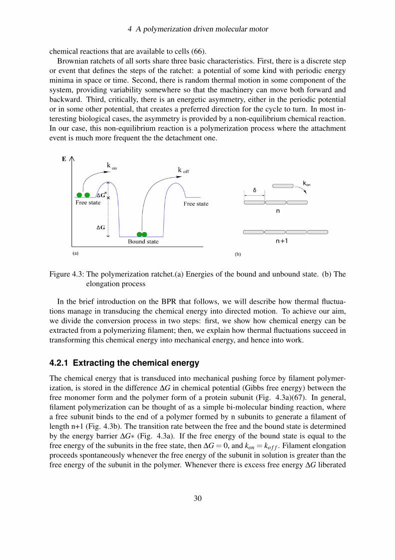
Figure 4.3: The polymerization ratchet.(a) Energies of the bound and unbound state. (b) Theelongation process
In the brief introduction on the BPR that follows, we will describe how thermal fluctua-tions manage in transducing the chemical energy into directed motion. To achieve our aim,we divide the conversion process in two steps: first, we show how chemical energy can beextracted from a polymerizing filament; then, we explain how thermal fluctuations succeed intransforming this chemical energy into mechanical energy, and hence into work.
4.2.1 Extracting the chemical energy
The chemical energy that is transduced into mechanical pushing force by filament polymer-ization, is stored in the difference ∆G in chemical potential (Gibbs free energy) between thefree monomer form and the polymer form of a protein subunit (Fig. 4.3a)(67). In general,filament polymerization can be thought of as a simple bi-molecular binding reaction, wherea free subunit binds to the end of a polymer formed by n subunits to generate a filament oflength n+1 (Fig. 4.3b). The transition rate between the free and the bound state is determinedby the energy barrier ∆G∗ (Fig. 4.3a). If the free energy of the bound state is equal to thefree energy of the subunits in the free state, then ∆G = 0, and kon = ko f f . Filament elongationproceeds spontaneously whenever the free energy of the subunit in solution is greater than thefree energy of the subunit in the polymer. Whenever there is excess free energy ∆G liberated
30
4 A polymerization driven molecular motor
from a chemical reaction, it can in principle be harnessed and converted into another form ofenergy.
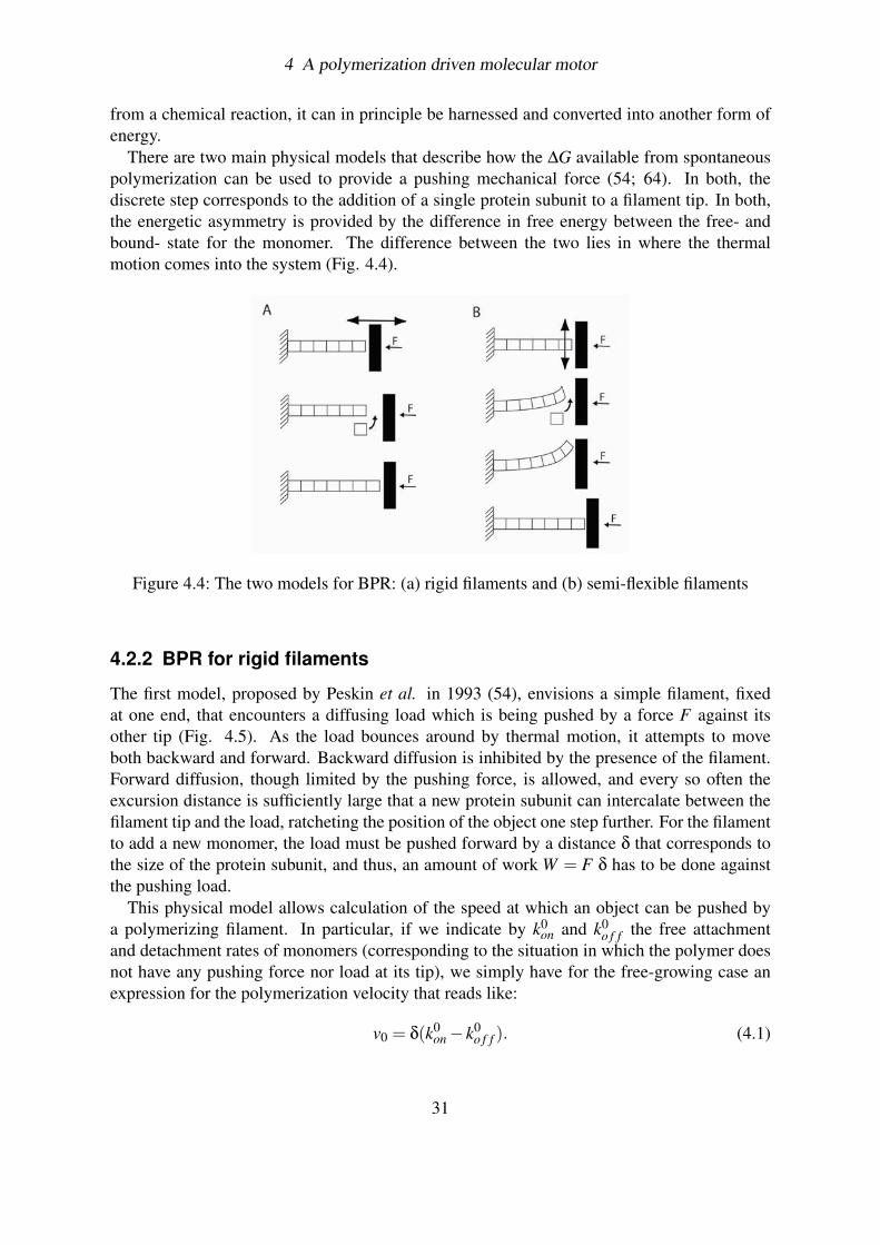
There are two main physical models that describe how the ∆G available from spontaneouspolymerization can be used to provide a pushing mechanical force (54; 64). In both, thediscrete step corresponds to the addition of a single protein subunit to a filament tip. In both,the energetic asymmetry is provided by the difference in free energy between the free- andbound- state for the monomer. The difference between the two lies in where the thermalmotion comes into the system (Fig. 4.4).
Figure 4.4: The two models for BPR: (a) rigid filaments and (b) semi-flexible filaments
4.2.2 BPR for rigid filaments
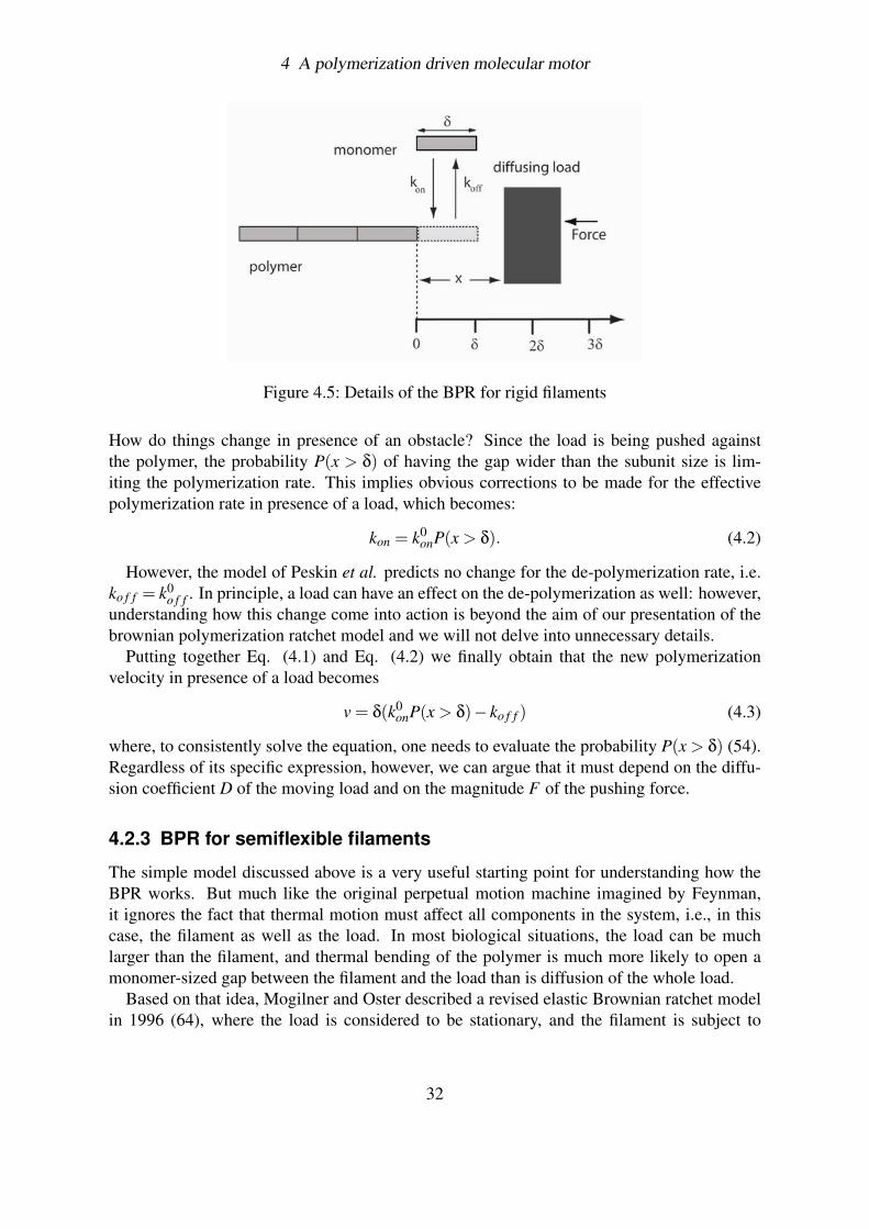
The first model, proposed by Peskin et al. in 1993 (54), envisions a simple filament, fixedat one end, that encounters a diffusing load which is being pushed by a force F against itsother tip (Fig. 4.5). As the load bounces around by thermal motion, it attempts to moveboth backward and forward. Backward diffusion is inhibited by the presence of the filament.Forward diffusion, though limited by the pushing force, is allowed, and every so often theexcursion distance is sufficiently large that a new protein subunit can intercalate between thefilament tip and the load, ratcheting the position of the object one step further. For the filamentto add a new monomer, the load must be pushed forward by a distance δ that corresponds tothe size of the protein subunit, and thus, an amount of work W = F δ has to be done againstthe pushing load.
This physical model allows calculation of the speed at which an object can be pushed bya polymerizing filament. In particular, if we indicate by k0
on and k0o f f the free attachment
and detachment rates of monomers (corresponding to the situation in which the polymer doesnot have any pushing force nor load at its tip), we simply have for the free-growing case anexpression for the polymerization velocity that reads like:
v0 = δ(k0on− k0
o f f ). (4.1)
31
4 A polymerization driven molecular motor
Figure 4.5: Details of the BPR for rigid filaments
How do things change in presence of an obstacle? Since the load is being pushed againstthe polymer, the probability P(x > δ) of having the gap wider than the subunit size is lim-iting the polymerization rate. This implies obvious corrections to be made for the effectivepolymerization rate in presence of a load, which becomes:
kon = k0onP(x > δ). (4.2)
However, the model of Peskin et al. predicts no change for the de-polymerization rate, i.e.ko f f = k0
o f f . In principle, a load can have an effect on the de-polymerization as well: however,understanding how this change come into action is beyond the aim of our presentation of thebrownian polymerization ratchet model and we will not delve into unnecessary details.
Putting together Eq. (4.1) and Eq. (4.2) we finally obtain that the new polymerizationvelocity in presence of a load becomes
v = δ(k0onP(x > δ)− ko f f ) (4.3)
where, to consistently solve the equation, one needs to evaluate the probability P(x > δ) (54).Regardless of its specific expression, however, we can argue that it must depend on the diffu-sion coefficient D of the moving load and on the magnitude F of the pushing force.
4.2.3 BPR for semiflexible filaments
The simple model discussed above is a very useful starting point for understanding how theBPR works. But much like the original perpetual motion machine imagined by Feynman,it ignores the fact that thermal motion must affect all components in the system, i.e., in thiscase, the filament as well as the load. In most biological situations, the load can be muchlarger than the filament, and thermal bending of the polymer is much more likely to open amonomer-sized gap between the filament and the load than is diffusion of the whole load.
Based on that idea, Mogilner and Oster described a revised elastic Brownian ratchet modelin 1996 (64), where the load is considered to be stationary, and the filament is subject to
32
4 A polymerization driven molecular motor
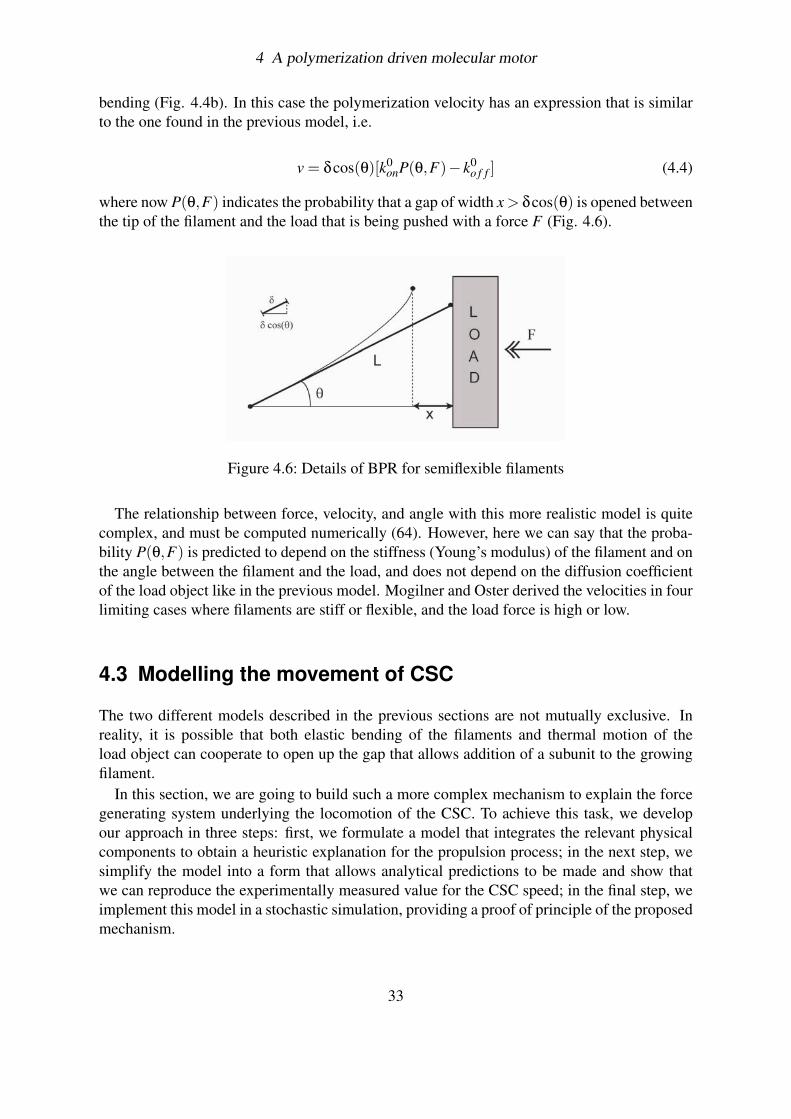
bending (Fig. 4.4b). In this case the polymerization velocity has an expression that is similarto the one found in the previous model, i.e.
v = δcos(θ)[k0onP(θ,F)− k0
o f f ] (4.4)
where now P(θ,F) indicates the probability that a gap of width x > δcos(θ) is opened betweenthe tip of the filament and the load that is being pushed with a force F (Fig. 4.6).
Figure 4.6: Details of BPR for semiflexible filaments
The relationship between force, velocity, and angle with this more realistic model is quitecomplex, and must be computed numerically (64). However, here we can say that the proba-bility P(θ,F) is predicted to depend on the stiffness (Young’s modulus) of the filament and onthe angle between the filament and the load, and does not depend on the diffusion coefficientof the load object like in the previous model. Mogilner and Oster derived the velocities in fourlimiting cases where filaments are stiff or flexible, and the load force is high or low.
4.3 Modelling the movement of CSC
The two different models described in the previous sections are not mutually exclusive. Inreality, it is possible that both elastic bending of the filaments and thermal motion of theload object can cooperate to open up the gap that allows addition of a subunit to the growingfilament.
In this section, we are going to build such a more complex mechanism to explain the forcegenerating system underlying the locomotion of the CSC. To achieve this task, we developour approach in three steps: first, we formulate a model that integrates the relevant physicalcomponents to obtain a heuristic explanation for the propulsion process; in the next step, wesimplify the model into a form that allows analytical predictions to be made and show thatwe can reproduce the experimentally measured value for the CSC speed; in the final step, weimplement this model in a stochastic simulation, providing a proof of principle of the proposedmechanism.
33
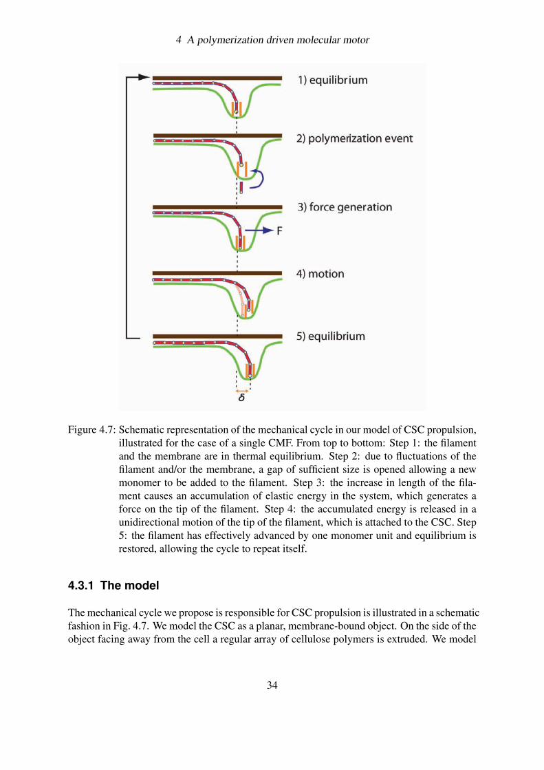
4 A polymerization driven molecular motor
Figure 4.7: Schematic representation of the mechanical cycle in our model of CSC propulsion,illustrated for the case of a single CMF. From top to bottom: Step 1: the filamentand the membrane are in thermal equilibrium. Step 2: due to fluctuations of thefilament and/or the membrane, a gap of sufficient size is opened allowing a newmonomer to be added to the filament. Step 3: the increase in length of the fila-ment causes an accumulation of elastic energy in the system, which generates aforce on the tip of the filament. Step 4: the accumulated energy is released in aunidirectional motion of the tip of the filament, which is attached to the CSC. Step5: the filament has effectively advanced by one monomer unit and equilibrium isrestored, allowing the cycle to repeat itself.
4.3.1 The model
The mechanical cycle we propose is responsible for CSC propulsion is illustrated in a schematicfashion in Fig. 4.7. We model the CSC as a planar, membrane-bound object. On the side of theobject facing away from the cell a regular array of cellulose polymers is extruded. We model
34
4 A polymerization driven molecular motor
these polymers as inextensible semiflexible chains of beads. The configuration of these poly-mers is constrained by three factors. The first is their attachment to the CSC itself. Here weassume that this attachment not only fixes the location of the polymer tips, but also specifiesthe orientation of their first bonds to be perpendicular to the plane of the CSC. The latter as-sumption is consistent with the hypothesis that the chains emerge from narrow channels in thecomplex. The second constraining factor is the confining influence of the already depositedcell wall, which we model as an impenetrable barrier. The final constraint arises from the factthat the polymers are at their other ends all linked up into a nascent CMF, which on this scaleis an effectively rigid linear structure constrained to lie in the plane of the membrane.
Because the polymers have a finite resistance to bending, the combination of geometricalconstraints imposed on them implies that they are in a non-relaxed conformation, resulting inforces acting on their attachment points. At the loci where the polymers emerge from the CSCthese forces will typically have both a perpendicular component and an in-plane component.The perpendicular component has two effects: (i) it acts as a barrier for the polymerizationprocess, thus influencing the rate of addition of new monomers, and (ii) it contributes to a netforce which pushes the CSC downward, counteracted by an elastic response of the membrane.The latter effect is consistent with the membrane-indentations that are seen in some freeze-fracture images of the CSC (68) (See also Fig.4.1). Note that we disregard the possibility thatthe CSC “tilts” with respect to the global membrane orientation, as the energetic cost of suchshort length-scale deformations of the membrane is probably appreciable.
The resultant of all the in-plane force components due to the individual polymers is thenet force that drives the linear motion of the CSC. Energy is injected into this system by thepolymerization- as well as the crystallization process, as both will tend to increase the stressin the polymers. The energy is dissipated by the work the CSC as a whole performs againstthe frictional forces it experiences. We stress the fact that thermal fluctuations, which area dominant effect at the relevant molecular scale, play a crucial role in the whole process,making possible the opening of a gap big enough for the insertion of a new polymer subunit.It is these fluctuations which allow the system to cross (and also to re-cross) the energeticbarriers associated with the mechanical constraints imposed on the polymerization process.Like in the BPRs models discussed in the previous sections, it is the rectification of thesefluctuations that allow the system to convert chemical energy into directed motion.
4.3.2 Analytical treatment
Now that we have illustrated how the proposed mechanism manages in pushing the CSCthrough the membrane, we undertake to strip the model to its bare essentials, focusing ona single growing polymer constrained to a 2D planar geometry interacting with an 3D elasticmembrane. In this simplified setting, whose projection on a vertical plane is already illus-trated in Fig. 4.7, the model can be solved exactly, allowing the polymerization velocity to bedetermined.
In our analytical picture the chain is modeled as a semiflexible filament with a persistencelength ξ f significantly larger than the typical dimensions of the region where the filament isbent. The membrane is fixed at its edges to a rigid frame of size Ω = l2, and its equilibrium po-sition is taken to coincide with the hard top wall which represents the already extant cell wall.
35
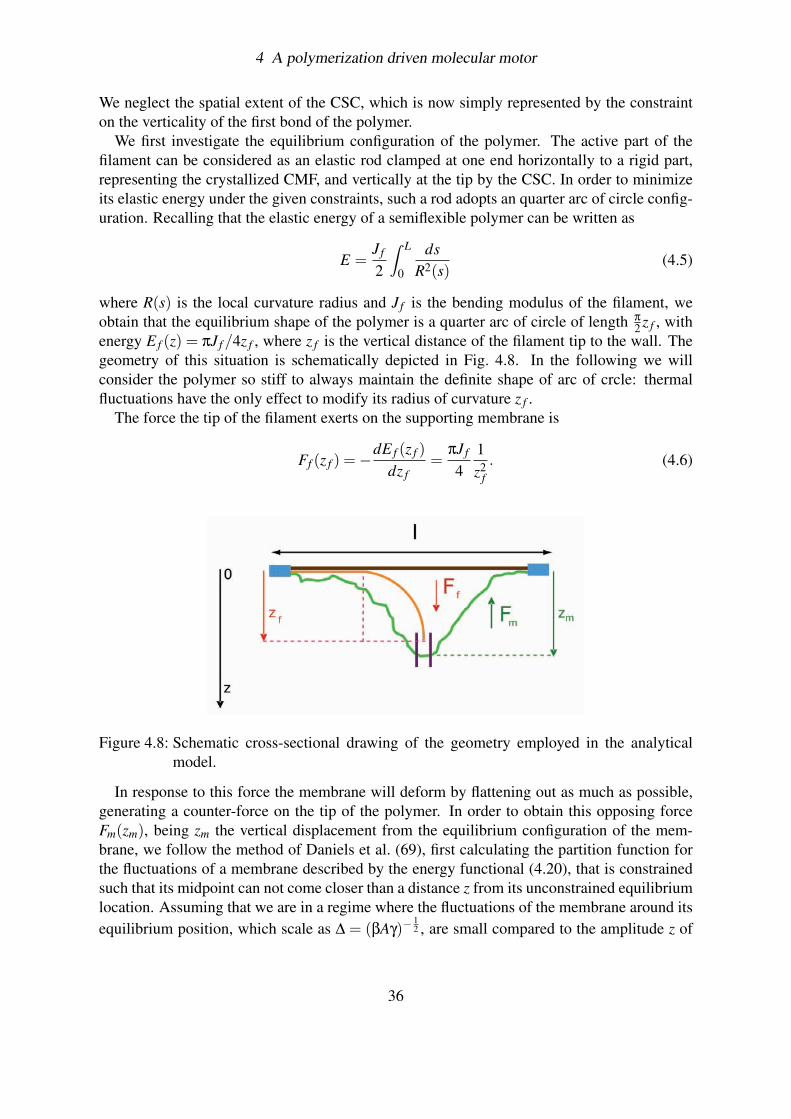
4 A polymerization driven molecular motor
We neglect the spatial extent of the CSC, which is now simply represented by the constrainton the verticality of the first bond of the polymer.
We first investigate the equilibrium configuration of the polymer. The active part of thefilament can be considered as an elastic rod clamped at one end horizontally to a rigid part,representing the crystallized CMF, and vertically at the tip by the CSC. In order to minimizeits elastic energy under the given constraints, such a rod adopts an quarter arc of circle config-uration. Recalling that the elastic energy of a semiflexible polymer can be written as
E =J f
2
Z L
0
dsR2(s)
(4.5)
where R(s) is the local curvature radius and J f is the bending modulus of the filament, weobtain that the equilibrium shape of the polymer is a quarter arc of circle of length π
2 z f , withenergy E f (z) = πJ f /4z f , where z f is the vertical distance of the filament tip to the wall. Thegeometry of this situation is schematically depicted in Fig. 4.8. In the following we willconsider the polymer so stiff to always maintain the definite shape of arc of crcle: thermalfluctuations have the only effect to modify its radius of curvature z f .
The force the tip of the filament exerts on the supporting membrane is
Ff (z f ) =−dE f (z f )
dz f=
πJ f
41z2
f. (4.6)
Figure 4.8: Schematic cross-sectional drawing of the geometry employed in the analyticalmodel.
In response to this force the membrane will deform by flattening out as much as possible,generating a counter-force on the tip of the polymer. In order to obtain this opposing forceFm(zm), being zm the vertical displacement from the equilibrium configuration of the mem-brane, we follow the method of Daniels et al. (69), first calculating the partition function forthe fluctuations of a membrane described by the energy functional (4.20), that is constrainedsuch that its midpoint can not come closer than a distance z from its unconstrained equilibriumlocation. Assuming that we are in a regime where the fluctuations of the membrane around itsequilibrium position, which scale as ∆ = (βAγ)−
12 , are small compared to the amplitude z of
36
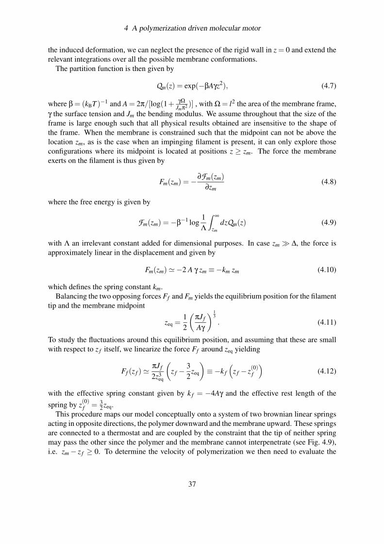
4 A polymerization driven molecular motor
the induced deformation, we can neglect the presence of the rigid wall in z = 0 and extend therelevant integrations over all the possible membrane conformations.
The partition function is then given by
Qm(z) = exp(−βAγz2), (4.7)
where β = (kBT )−1 and A = 2π/[log(1+ γΩ
Jmπ2 )] , with Ω = l2 the area of the membrane frame,γ the surface tension and Jm the bending modulus. We assume throughout that the size of theframe is large enough such that all physical results obtained are insensitive to the shape ofthe frame. When the membrane is constrained such that the midpoint can not be above thelocation zm, as is the case when an impinging filament is present, it can only explore thoseconfigurations where its midpoint is located at positions z ≥ zm. The force the membraneexerts on the filament is thus given by
Fm(zm) =−∂Fm(zm)∂zm
(4.8)
where the free energy is given by
Fm(zm) =−β−1 log
1Λ
Z∞
zm
dzQm(z) (4.9)
with Λ an irrelevant constant added for dimensional purposes. In case zm ∆, the force isapproximately linear in the displacement and given by
Fm(zm)'−2 A γ zm ≡−km zm (4.10)
which defines the spring constant km.Balancing the two opposing forces Ff and Fm yields the equilibrium position for the filament
tip and the membrane midpoint
zeq =12
(πJ f
Aγ
) 13
. (4.11)
To study the fluctuations around this equilibrium position, and assuming that these are smallwith respect to z f itself, we linearize the force Ff around zeq yielding
Ff (z f )'πJ f
2z3eq
(z f −
32
zeq
)≡−k f
(z f − z(0)
f
)(4.12)
with the effective spring constant given by k f = −4Aγ and the effective rest length of thespring by z(0)
f = 32zeq.
This procedure maps our model conceptually onto a system of two brownian linear springsacting in opposite directions, the polymer downward and the membrane upward. These springsare connected to a thermostat and are coupled by the constraint that the tip of neither springmay pass the other since the polymer and the membrane cannot interpenetrate (see Fig. 4.9),i.e. zm− z f ≥ 0. To determine the velocity of polymerization we then need to evaluate the
37
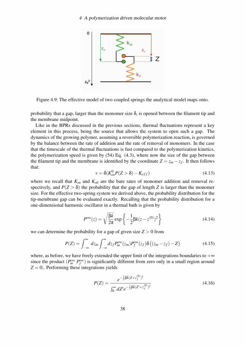
4 A polymerization driven molecular motor
Figure 4.9: The effective model of two coupled springs the analytical model maps onto.
probability that a gap, larger than the monomer size δ, is opened between the filament tip andthe membrane midpoint.
Like in the BPRs discussed in the previous sections, thermal fluctuations represent a keyelement in this process, being the source that allows the system to open such a gap. Thedynamics of the growing polymer, assuming a reversible polymerization reaction, is governedby the balance between the rate of addition and the rate of removal of monomers. In the casethat the timescale of the thermal fluctuations is fast compared to the polymerization kinetics,the polymerization speed is given by (54) Eq. (4.3), where now the size of the gap betweenthe filament tip and the membrane is identified by the coordinate Z = zm− z f . It then followsthat:
v = δ(K0onP(Z > δ)−Ko f f ) (4.13)
where we recall that Kon and Koff are the bare rates of monomer addition and removal re-spectively, and P(Z > δ) the probability that the gap of length Z is larger than the monomersize. For the effective two-spring system we derived above, the probability distribution for thetip-membrane gap can be evaluated exactly. Recalling that the probability distribution for aone-dimensional harmonic oscillator in a thermal bath is given by
Posc(z) =
√βk2π
exp−1
2βk(z− z(0))2
(4.14)
we can determine the probability for a gap of given size Z > 0 from
P(Z) =Z
∞
−∞
dzm
Z∞
−∞
dz f Poscm (zm)Posc
f (z f )δ((zm− z f )−Z
)(4.15)
where, as before, we have freely extended the upper limit of the integrations boundaries to +∞
since the product (Poscm Posc
f ) is significantly different from zero only in a small region aroundZ = 0;. Performing these integrations yields
P(Z) =e−
12 βk(Z+z(0)
f )2
R∞
0 dZ′e−12 βk(Z′+z(0)
f )2(4.16)
38
4 A polymerization driven molecular motor
where the effective spring constant of the coupled system is given by k = kmk f /(km + k f ). Inorder to assess the validity of the approximations made in deriving the analytical model, wecompare the prediction of the gap distribution in Eq. (4.16) with the results we obtain fromsampling of a one-filament version of the full stochastic model that will be presented in section4.3.3. The results are presented in Fig. 4.10 and show a perfect agreement.
Eq. (4.16) in turns allows the explicit evaluation of the probability that the gap is larger thanthe monomer size
P(Z > δ) =Z
∞
δ
dZ′P(Z′) =1+ erf
(√12βk (z(0)
f −δ))
1+ erf(√
12βk z(0)
f
) (4.17)
where erf(x) is the error function, z(0)f the equilibrium position of the linearized polymer-
spring, k an effective spring constant and β = 1/kBT the standard inverse temperature. Takentogether, Eqs. (4.13) and (4.17) allow the polymerization velocity, which equals the velocityof motion of the CSC, to be determined as a function of all the relevant parameters. Deferringthe numerical estimate of this velocity to the next section, we remark that we can readilydeduce that the polymerization velocity increases with increasing temperature and decreaseswith increasing stiffness of the system, caused either by increased stiffness of the filaments orthe membrane. Interestingly the former consideration is backed up with experimental evidence(unpublished data, Brown lab).
4.3.2.1 Results
We can now employ the results obtained through this analytical approach to estimate the ve-locity of the CSC. In this attempt we are of course limited by the availability of quantitativeestimates of the relevant parameters.
We first consider the bending modulus of the effective filament, arguably the least welldetermined parameter. Using crystallographic data we can provide an upper and a lower boundto the value of J f as the Young’s modulus Y of cellulose is known to vary between 5 GPa for theamorphous state and 150 GPa for the crystalline state (70). We can, however, extract a moreappropriate estimate from the depth of the observed indentation of the plasma membrane at thelocus of the CSC, which provides an estimate for the equilibrium value of the filament tip towall distance zeq. Through the use of relation Eq. (4.11) we can then determine J f = 8 Aγz3
eq/π.For typical values of the membrane surface tension γ = 5×10⁻⁵ N/m, the membrane bendingmodulus Jm = 2× 10⁻²⁰ Nm, an indentation depth of zeq = 100 nm and size of the relevantmembrane patch l≈ 300 nm, we find J f = 2.5×10⁻²⁵ Pa m4. Taking the radius of the effectivefilament to be r = 1/2 diameter of CMF = 2nm, we obtain an estimate of Y = 4J f /(πr4) =20 Gpa, which falls squarely between the bounds mentioned above. We have to keep in mindthat, even if the structure of the CMF is almost perfectly crystalline, at the moment of theextrusion from the CSC the glucan chain aggregates are in a non-crystallized phase. Thus theeffective Young’s modulus of the aggregate is much lower that the one of a cellulose crystal.
For the polymerization rate we use the value of free polymerization of cellulose achieved bythe bacterium Acetobacter, the so-called vinegar bacterium that lives at the water-air interface
39
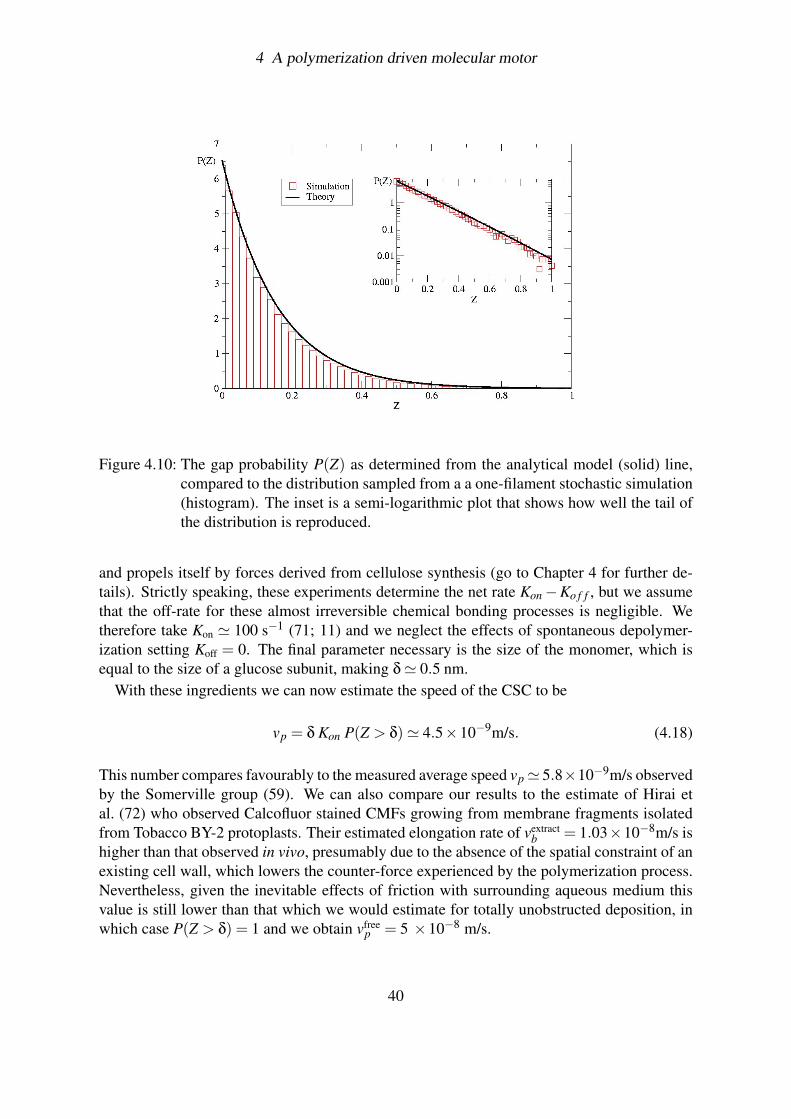
4 A polymerization driven molecular motor
Figure 4.10: The gap probability P(Z) as determined from the analytical model (solid) line,compared to the distribution sampled from a a one-filament stochastic simulation(histogram). The inset is a semi-logarithmic plot that shows how well the tail ofthe distribution is reproduced.
and propels itself by forces derived from cellulose synthesis (go to Chapter 4 for further de-tails). Strictly speaking, these experiments determine the net rate Kon−Ko f f , but we assumethat the off-rate for these almost irreversible chemical bonding processes is negligible. Wetherefore take Kon ' 100 s−1 (71; 11) and we neglect the effects of spontaneous depolymer-ization setting Koff = 0. The final parameter necessary is the size of the monomer, which isequal to the size of a glucose subunit, making δ' 0.5 nm.
With these ingredients we can now estimate the speed of the CSC to be
vp = δ Kon P(Z > δ)' 4.5×10⁻⁹m/s. (4.18)
This number compares favourably to the measured average speed vp' 5.8×10⁻⁹m/s observedby the Somerville group (59). We can also compare our results to the estimate of Hirai etal. (72) who observed Calcofluor stained CMFs growing from membrane fragments isolatedfrom Tobacco BY-2 protoplasts. Their estimated elongation rate of vextract
b = 1.03×10⁻⁸m/s ishigher than that observed in vivo, presumably due to the absence of the spatial constraint of anexisting cell wall, which lowers the counter-force experienced by the polymerization process.Nevertheless, given the inevitable effects of friction with surrounding aqueous medium thisvalue is still lower than that which we would estimate for totally unobstructed deposition, inwhich case P(Z > δ) = 1 and we obtain vfree
p = 5 ×10⁻⁸ m/s.
40
4 A polymerization driven molecular motor
4.3.3 Stochastic simulation
We now implement the conceptual model presented in sect. 4.3.1 in terms of a stochasticsimulation. In the following, even though the simulated systems are discretized for numer-ical purposes, we will express their Hamiltonians in the continuum limit. The Monte Carloscheme used in the stochastic simulation consists of a series of stochastic transitions betweendifferent system configurations, all satisfying the imposed constraints. The probability of agiven transition depends on the energy difference between the two successive configurationsand satisfies the detailed balance condition that ensures the correct sampling of the equilibriumphase space.
For simplicity we consider a CSC producing 6 effective filaments (EFs), each representing6 cellulose chains. This simplification is consistent with the mechanism proposed by Cousinset al. (13) in which the approximately 36 cellulose strands that emerge from the CSC are firstassembled into 6 glucan chain aggregates, which subsequently coalesce crystallizing into aCMF. The EFs are modelled as bead-chains with a bending potential governing the relativeorientation of pairs of neighboring bonds. Each filament is represented as a discrete linearchain of N f spherical beads of diameter σ that are rigidly connected by bonds of fixed lengthδ = σ. The length of each chain is thus l fi = N fiσ, where the subscript i = (1..6) refers tothe i-th filament. The angular bending potential between two subsequent bonds in the chainis given by U(θ) = J f [1− cos(θ)], where θ is the angle and J f is the bending constant thatdetermines the stiffness of the filament.
The already extant cell wall is taken to be a rigid wall located at z = 0, into which thebeads are not allowed to enter. The EFs emerge from six hexagonally arranged channelsrepresenting the CSC. The first monomer-monomer bond (tip) of each filament is constrainedto be perpendicular to the plane of the CSC (i.e. is oriented along the vertical axis of thelaboratory frame) while the last monomer-monomer bond (tail) is parallel to the horizontalaxis. Because of the morphology of the CSC, the tips of the filaments are also constrained tobe located at the vertexes of a regular hexagon, with edge-length Rhex = 6σ. In addition, thebeads on different chains have a short range attractive interaction allowing them to crystallizeinto a compact arrangement.
The individual filaments can be described by inextensible space curves r(s), where s is thearc-length parameter. The constraint of inextensibility implies that d
dsr(s) = 0, so that the
local curvature of a filament is given by κ(s) =∣∣∣ d2
ds2 r(s)∣∣∣. In the absence of the constraints, the
Hamiltonian for the full bundle of 6 filaments is then given by
H bundlep =
12
J f
6
∑i=1
Z l fi
0dsiκi(si)− εσ
−2∑
1≤i< j≤6
Z l fi
0dsi
Z l f j
0ds j θ
(√2σ−
∣∣ri(si)− r j(s j)∣∣)
(4.19)where the binding energy ε is attributed to each pair of monomers on different filaments thatare closer than the attraction radius
√2σ.
The whole construct (EF+hexagon) interacts with a fluid membrane modelled as a dynam-ically reconfigurable squared network of beads and springs. The liquid bilayer is representedas a l× l grid of N2
m point particles of size σ that are capable of moving only in the verti-cal direction. The edges of the membrane are kept fixed at z = 0. The Hamiltonian for the
41
4 A polymerization driven molecular motor
membrane is described by the Helfrich functional (73)
Hm =Z (Jm
2(∇2h)2 +
γ
2(∇h)2
)dxdy (4.20)
where h is the local vertical distance with respect to the equilibrium position, Jm the bendingmodulus, γ the surface tension contribution and the integration runs over the area of the mem-brane. This Hamiltonian is the base-model to describe lipid bilayers, since such membranesare fluid in their lateral direction but resistant to stretching forces due to the hydrophobic ef-fect. In this model we neglect the internal pressure P of the cell, since it has been shown thatit makes only a trivial contribution (74).
The fact that the tips of the EFs cannot penetrate the membrane, couples the EFs energeti-cally to the membrane. Starting from an initial condition in which the end of one of the chainsis clamped, the simulation now proceeds as follows. An attempt is made to move one of theparticles in the system (either a chain or a membrane bead). The proposed movement is ac-cepted with a probability proportional to the Boltzmann weight of the associated change inenergy of the whole system (including the energies associated with various constraints). Thisprocedure is then repeated for several sweeps over all the particles in the system. This stan-dard Metropolis Monte Carlo scheme allows the system to equilibrate its state to the currentlengths of the individuals EFs. After this equilibration step, the gap between the tips of theEFs and the membrane is monitored for all the EFs. If this gap is larger than the size of achain bead, a new bead is added at the tip, preserving the perpendicular orientation of the firstbond. The system is then allowed to equilibrate again, and the whole cycle is repeated. Notethat this algorithm is a microscopic implementation of a Brownian ratchet, in the case that thefluctuations are fast compared to the polymerization rate.
4.3.3.1 Results
The results of our simulation show that after initial effects have died down, a stationary regimeis reached in which the CSC moves with a statistically stationary velocity in a direction dic-tated by the essentially straight CMF produced. This shows that indeed, the polymerizationand crystallization processes, both exothermic, coupled by thermal fluctuations to the mem-brane and the partially flexible chains as energy transducers, are sufficient to obtain the di-rected motion of the synthase.
Fig. 4.11 shows four snapshots of our simulation at successive times. We note that althoughthe trajectory of the CSC is approximately linear, the complex itself undergoes a rotationduring its motion. This is caused by the helical nature of the crystalline structure of ourpseudo-CMF, which is a natural consequence of the maximization of the binding energy. In-triguingly, cellulose microfibrils have also been observed experimentally to "twist" (75; 76),an effect generally attributed to the chirality of the planar glucan chains, which spontaneously“twist” to relieve the strain built around the oxygen bridge that holds the glucan together. Clearevidence of this phenomenon is given by the twisted cellulose ribbon produced by the Aceto-bacter, whose cells move undergoing a continuous rotation on their longitudinal axis: this iscaused by the relieving of the stress induced by the non-linear crystallization of the nascentglucan chains during the biogenesis of the CMF (18). Also clearly visible in the side views of
42
4 A polymerization driven molecular motor
Fig. 4.11 is the marked indentation of the membrane at the locus of CSC, over an area severaltimes the area of the complex itself. This indentation is a consequence of the forces generatedby the bent EFs, and has been observed experimentally (see Fig. 4.1 and (68)), and as suchprovides direct evidence in favour of our model.
4.4 Conclusions
The model proposed for the mechanism of the CSC propulsion in this chapter achieves threegoals. First of all, on a conceptual level it provides an explicit and physically consistentheuristic for understanding CSC motion. Secondly, the analytical approach, which abstractsthe model to its bare essentials, allows the observable result of the mechanism, i.e. the velocityof motion of the CSC, to be quantified in terms of the underlying physico-chemical parameters.Finally, our stochastic simulations, albeit simplified with respect to reality, provide a proof ofprinciple of this mechanism. The fundamental assumption of the model, i.e. the microscopicfluctuations occur on timescale fast compared to that of the motion of the CSC, justifies theuse of the coarse graining that underlies the analytical approach: this manages in replacing themany individual microscopic degrees of freedom with a small number of effective ones.
We contend that the biophysical model presented here provides a solid basis for understand-ing the propulsion of an individual CSC . Moreover, it gives an estimate for the polymerizationvelocity of the CMF that is consistent with the observed speed of the CSC within the uncer-tainty imposed by the approximations used. This opens the way for considering the muchmore challenging problem of understanding the full dynamics of cell wall deposition, whichinvolves the simultaneous and apparently highly coordinated deposition of many CMFs. In-deed, the question of the origin of the highly regular CMF textures found in secondary cellwalls is still actively debated. Whilst the textbook explanation involves the guidance of CSCsby ordered arrays of cortical microtubules (77), there is also a body of evidence against thisidea, and a few models have been suggested that rely more strongly on the physical inter-actions between the CSCs and the CMFs they produce (see e.g (78; 79)). Clearly, all theseapproaches will benefit from a fuller understanding of the motive processes of the CSC ininteraction with its direct environment.
43
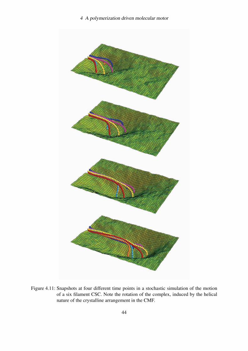
4 A polymerization driven molecular motor
Figure 4.11: Snapshots at four different time points in a stochastic simulation of the motionof a six filament CSC. Note the rotation of the complex, induced by the helicalnature of the crystalline arrangement in the CMF.
44
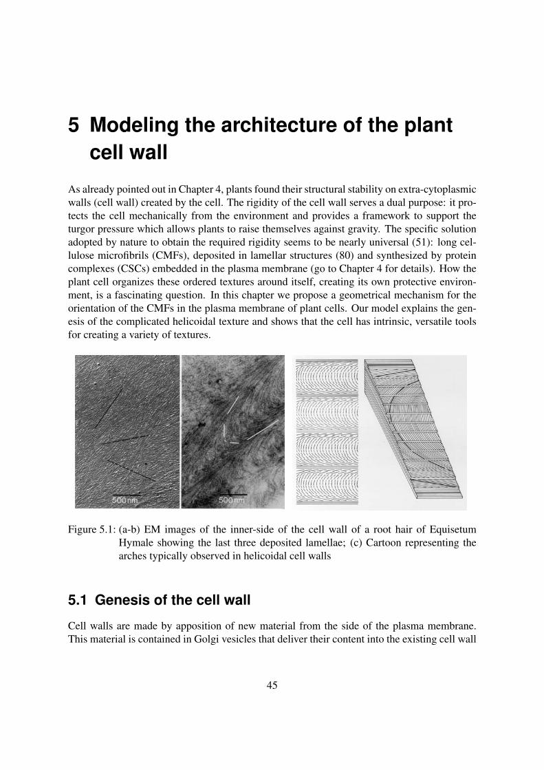
5 Modeling the architecture of the plantcell wall
As already pointed out in Chapter 4, plants found their structural stability on extra-cytoplasmicwalls (cell wall) created by the cell. The rigidity of the cell wall serves a dual purpose: it pro-tects the cell mechanically from the environment and provides a framework to support theturgor pressure which allows plants to raise themselves against gravity. The specific solutionadopted by nature to obtain the required rigidity seems to be nearly universal (51): long cel-lulose microfibrils (CMFs), deposited in lamellar structures (80) and synthesized by proteincomplexes (CSCs) embedded in the plasma membrane (go to Chapter 4 for details). How theplant cell organizes these ordered textures around itself, creating its own protective environ-ment, is a fascinating question. In this chapter we propose a geometrical mechanism for theorientation of the CMFs in the plasma membrane of plant cells. Our model explains the gen-esis of the complicated helicoidal texture and shows that the cell has intrinsic, versatile toolsfor creating a variety of textures.
Figure 5.1: (a-b) EM images of the inner-side of the cell wall of a root hair of EquisetumHymale showing the last three deposited lamellae; (c) Cartoon representing thearches typically observed in helicoidal cell walls
5.1 Genesis of the cell wall
Cell walls are made by apposition of new material from the side of the plasma membrane.This material is contained in Golgi vesicles that deliver their content into the existing cell wall
45
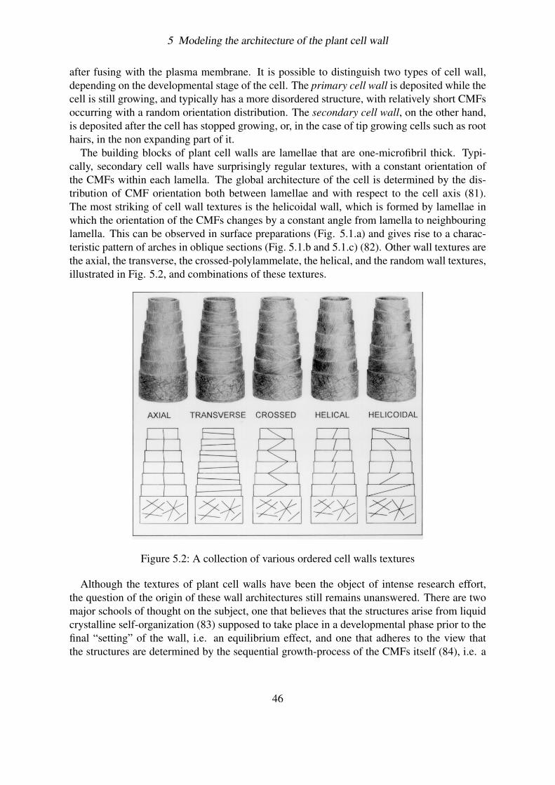
5 Modeling the architecture of the plant cell wall
after fusing with the plasma membrane. It is possible to distinguish two types of cell wall,depending on the developmental stage of the cell. The primary cell wall is deposited while thecell is still growing, and typically has a more disordered structure, with relatively short CMFsoccurring with a random orientation distribution. The secondary cell wall, on the other hand,is deposited after the cell has stopped growing, or, in the case of tip growing cells such as roothairs, in the non expanding part of it.
The building blocks of plant cell walls are lamellae that are one-microfibril thick. Typi-cally, secondary cell walls have surprisingly regular textures, with a constant orientation ofthe CMFs within each lamella. The global architecture of the cell is determined by the dis-tribution of CMF orientation both between lamellae and with respect to the cell axis (81).The most striking of cell wall textures is the helicoidal wall, which is formed by lamellae inwhich the orientation of the CMFs changes by a constant angle from lamella to neighbouringlamella. This can be observed in surface preparations (Fig. 5.1.a) and gives rise to a charac-teristic pattern of arches in oblique sections (Fig. 5.1.b and 5.1.c) (82). Other wall textures arethe axial, the transverse, the crossed-polylammelate, the helical, and the random wall textures,illustrated in Fig. 5.2, and combinations of these textures.
Figure 5.2: A collection of various ordered cell walls textures
Although the textures of plant cell walls have been the object of intense research effort,the question of the origin of these wall architectures still remains unanswered. There are twomajor schools of thought on the subject, one that believes that the structures arise from liquidcrystalline self-organization (83) supposed to take place in a developmental phase prior to thefinal “setting” of the wall, i.e. an equilibrium effect, and one that adheres to the view thatthe structures are determined by the sequential growth-process of the CMFs itself (84), i.e. a
46
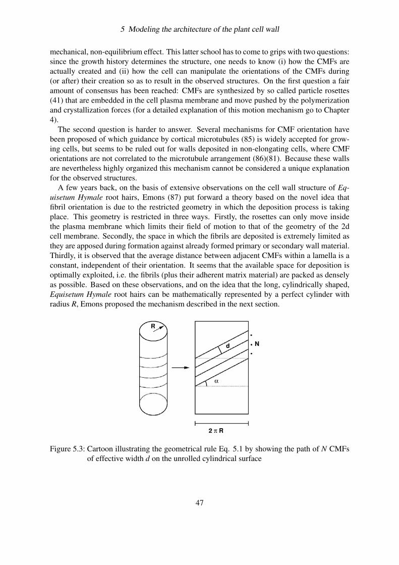
5 Modeling the architecture of the plant cell wall
mechanical, non-equilibrium effect. This latter school has to come to grips with two questions:since the growth history determines the structure, one needs to know (i) how the CMFs areactually created and (ii) how the cell can manipulate the orientations of the CMFs during(or after) their creation so as to result in the observed structures. On the first question a fairamount of consensus has been reached: CMFs are synthesized by so called particle rosettes(41) that are embedded in the cell plasma membrane and move pushed by the polymerizationand crystallization forces (for a detailed explanation of this motion mechanism go to Chapter4).
The second question is harder to answer. Several mechanisms for CMF orientation havebeen proposed of which guidance by cortical microtubules (85) is widely accepted for grow-ing cells, but seems to be ruled out for walls deposited in non-elongating cells, where CMForientations are not correlated to the microtubule arrangement (86)(81). Because these wallsare nevertheless highly organized this mechanism cannot be considered a unique explanationfor the observed structures.
A few years back, on the basis of extensive observations on the cell wall structure of Eq-uisetum Hymale root hairs, Emons (87) put forward a theory based on the novel idea thatfibril orientation is due to the restricted geometry in which the deposition process is takingplace. This geometry is restricted in three ways. Firstly, the rosettes can only move insidethe plasma membrane which limits their field of motion to that of the geometry of the 2dcell membrane. Secondly, the space in which the fibrils are deposited is extremely limited asthey are apposed during formation against already formed primary or secondary wall material.Thirdly, it is observed that the average distance between adjacent CMFs within a lamella is aconstant, independent of their orientation. It seems that the available space for deposition isoptimally exploited, i.e. the fibrils (plus their adherent matrix material) are packed as denselyas possible. Based on these observations, and on the idea that the long, cylindrically shaped,Equisetum Hymale root hairs can be mathematically represented by a perfect cylinder withradius R, Emons proposed the mechanism described in the next section.
Figure 5.3: Cartoon illustrating the geometrical rule Eq. 5.1 by showing the path of N CMFsof effective width d on the unrolled cylindrical surface
47
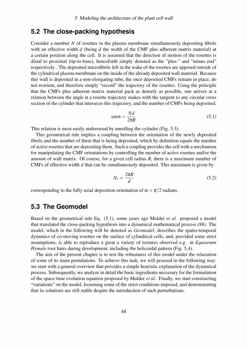
5 Modeling the architecture of the plant cell wall
5.2 The close-packing hypothesis
Consider a number N of rosettes in the plasma membrane simultaneously depositing fibrilswith an effective width d (being d the width of the CMF plus adherent matrix material) ata certain position along the cell. It is assumed that the direction of motion of the rosettes isdistal to proximal (tip-to-base), henceforth simply denoted as the ”plus-” and ”minus end”respectively . The deposited microfibrils left in the wake of the rosettes are apposed outside ofthe cylindrical plasma membrane on the inside of the already deposited wall material. Becausethis wall is deposited in a non-elongating tube, the once deposited CMFs remain in place, donot reorient, and therefore simply “record” the trajectory of the rosettes. Using the principlethat the CMFs plus adherent matrix material pack as densely as possible, one arrives at arelation between the angle α a rosette trajectory makes with the tangent to any circular crosssection of the cylinder that intersects this trajectory, and the number of CMFs being deposited.
sinα =Nd2πR
(5.1)
This relation is most easily understood by unrolling the cylinder (Fig. 5.3).This geometrical rule implies a coupling between the orientation of the newly deposited
fibrils and the number of them that is being deposited, which by definition equals the numberof active rosettes that are depositing them. Such a coupling provides the cell with a mechanismfor manipulating the CMF orientations by controlling the number of active rosettes and/or theamount of wall matrix. Of course, for a given cell radius R, there is a maximum number ofCMFs of effective width d that can be simultaneously deposited. This maximum is given by
N∗ =2πR
d(5.2)
corresponding to the fully axial deposition orientation of α = π/2 radians.
5.3 The Geomodel
Based on the geometrical rule Eq. (5.1), some years ago Mulder et al. proposed a modelthat translated the close-packing hypothesis into a dynamical mathematical process (88). Themodel, which in the following will be denoted as Geomodel, describes the spatio-temporaldynamics of co-moving rosettes on the surface of cylindrical cells, and, provided some strictassumptions, is able to reproduce a great a variety of textures observed e.g. in EquisetumHymale root hairs during development, including the helicoidal pattern (Fig. 5.4).
The aim of the present chapter is to test the robustness of this model under the relaxationof some of its main postulations. To achieve this task, we will proceed in the following way:we start with a general overview that provides a simple heuristic explanation of the dynamicalprocess. Subsequently, we analyze in detail the basic ingredients necessary for the formulationof the space-time evolution equation proposed by Mulder et al.. Finally, we start constructing“variations” on the model, loosening some of the strict conditions imposed, and demonstratingthat its solutions are still stable despite the introduction of such perturbations.
48
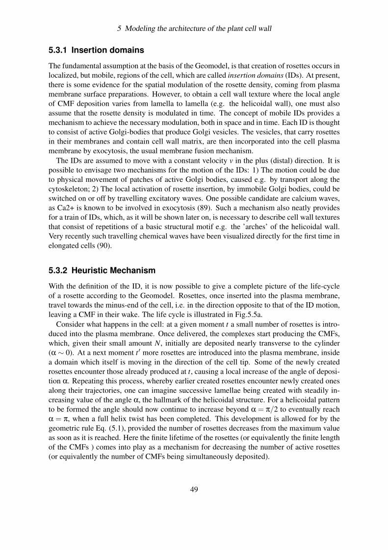
5 Modeling the architecture of the plant cell wall
5.3.1 Insertion domains
The fundamental assumption at the basis of the Geomodel, is that creation of rosettes occurs inlocalized, but mobile, regions of the cell, which are called insertion domains (IDs). At present,there is some evidence for the spatial modulation of the rosette density, coming from plasmamembrane surface preparations. However, to obtain a cell wall texture where the local angleof CMF deposition varies from lamella to lamella (e.g. the helicoidal wall), one must alsoassume that the rosette density is modulated in time. The concept of mobile IDs provides amechanism to achieve the necessary modulation, both in space and in time. Each ID is thoughtto consist of active Golgi-bodies that produce Golgi vesicles. The vesicles, that carry rosettesin their membranes and contain cell wall matrix, are then incorporated into the cell plasmamembrane by exocytosis, the usual membrane fusion mechanism.
The IDs are assumed to move with a constant velocity v in the plus (distal) direction. It ispossible to envisage two mechanisms for the motion of the IDs: 1) The motion could be dueto physical movement of patches of active Golgi bodies, caused e.g. by transport along thecytoskeleton; 2) The local activation of rosette insertion, by immobile Golgi bodies, could beswitched on or off by travelling excitatory waves. One possible candidate are calcium waves,as Ca2+ is known to be involved in exocytosis (89). Such a mechanism also neatly providesfor a train of IDs, which, as it will be shown later on, is necessary to describe cell wall texturesthat consist of repetitions of a basic structural motif e.g. the ’arches’ of the helicoidal wall.Very recently such travelling chemical waves have been visualized directly for the first time inelongated cells (90).
5.3.2 Heuristic Mechanism
With the definition of the ID, it is now possible to give a complete picture of the life-cycleof a rosette according to the Geomodel. Rosettes, once inserted into the plasma membrane,travel towards the minus-end of the cell, i.e. in the direction opposite to that of the ID motion,leaving a CMF in their wake. The life cycle is illustrated in Fig.5.5a.
Consider what happens in the cell: at a given moment t a small number of rosettes is intro-duced into the plasma membrane. Once delivered, the complexes start producing the CMFs,which, given their small amount N, initially are deposited nearly transverse to the cylinder(α ∼ 0). At a next moment t ′ more rosettes are introduced into the plasma membrane, insidea domain which itself is moving in the direction of the cell tip. Some of the newly createdrosettes encounter those already produced at t, causing a local increase of the angle of deposi-tion α. Repeating this process, whereby earlier created rosettes encounter newly created onesalong their trajectories, one can imagine successive lamellae being created with steadily in-creasing value of the angle α, the hallmark of the helicoidal structure. For a helicoidal patternto be formed the angle should now continue to increase beyond α = π/2 to eventually reachα = π, when a full helix twist has been completed. This development is allowed for by thegeometric rule Eq. (5.1), provided the number of rosettes decreases from the maximum valueas soon as it is reached. Here the finite lifetime of the rosettes (or equivalently the finite lengthof the CMFs ) comes into play as a mechanism for decreasing the number of active rosettes(or equivalently the number of CMFs being simultaneously deposited).
49
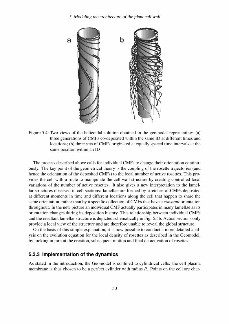
5 Modeling the architecture of the plant cell wall
Figure 5.4: Two views of the helicoidal solution obtained in the geomodel representing: (a)three generations of CMFs co-deposited within the same ID at different times andlocations; (b) three sets of CMFs originated at equally spaced time intervals at thesame position within an ID
The process described above calls for individual CMFs to change their orientation continu-ously. The key point of the geometrical theory is the coupling of the rosette trajectories (andhence the orientation of the deposited CMFs) to the local number of active rosettes. This pro-vides the cell with a route to manipulate the cell wall structure by creating controlled localvariations of the number of active rosettes. It also gives a new interpretation to the lamel-lar structures observed in cell sections: lamellae are formed by stretches of CMFs depositedat different moments in time and different locations along the cell that happen to share thesame orientation, rather than by a specific collection of CMFs that have a constant orientationthroughout. In the new picture an individual CMF actually participates in many lamellae as itsorientation changes during its deposition history. This relationship between individual CMFsand the resultant lamellar structure is depicted schematically in Fig. 5.5b. Actual sections onlyprovide a local view of the structure and are therefore unable to reveal the global structure.
On the basis of this simple explanation, it is now possible to conduct a more detailed anal-ysis on the evolution equation for the local density of rosettes as described in the Geomodel,by looking in turn at the creation, subsequent motion and final de-activation of rosettes.
5.3.3 Implementation of the dynamics
As stated in the introduction, the Geomodel is confined to cylindrical cells: the cell plasmamembrane is thus chosen to be a perfect cylinder with radius R. Points on the cell are char-
50
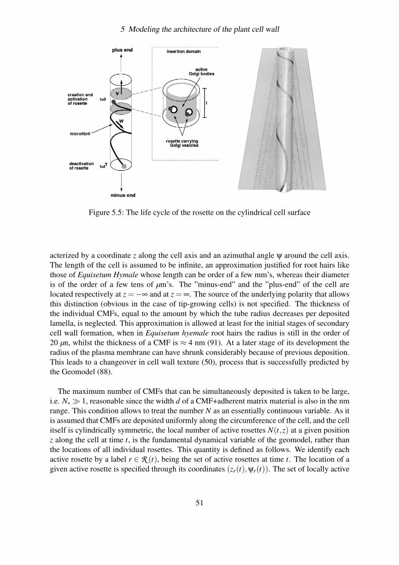
5 Modeling the architecture of the plant cell wall
Figure 5.5: The life cycle of the rosette on the cylindrical cell surface
acterized by a coordinate z along the cell axis and an azimuthal angle ψ around the cell axis.The length of the cell is assumed to be infinite, an approximation justified for root hairs likethose of Equisetum Hymale whose length can be order of a few mm’s, whereas their diameteris of the order of a few tens of µm’s. The ”minus-end” and the ”plus-end” of the cell arelocated respectively at z =−∞ and at z = ∞. The source of the underlying polarity that allowsthis distinction (obvious in the case of tip-growing cells) is not specified. The thickness ofthe individual CMFs, equal to the amount by which the tube radius decreases per depositedlamella, is neglected. This approximation is allowed at least for the initial stages of secondarycell wall formation, when in Equisetum hyemale root hairs the radius is still in the order of20 µn, whilst the thickness of a CMF is ≈ 4 nm (91). At a later stage of its development theradius of the plasma membrane can have shrunk considerably because of previous deposition.This leads to a changeover in cell wall texture (50), process that is successfully predicted bythe Geomodel (88).
The maximum number of CMFs that can be simultaneously deposited is taken to be large,i.e. N∗ 1, reasonable since the width d of a CMF+adherent matrix material is also in the nmrange. This condition allows to treat the number N as an essentially continuous variable. As itis assumed that CMFs are deposited uniformly along the circumference of the cell, and the cellitself is cylindrically symmetric, the local number of active rosettes N(t,z) at a given positionz along the cell at time t, is the fundamental dynamical variable of the geomodel, rather thanthe locations of all individual rosettes. This quantity is defined as follows. We identify eachactive rosette by a label r ∈ R (t), being the set of active rosettes at time t. The location of agiven active rosette is specified through its coordinates (zr(t),ψr(t)). The set of locally active
51
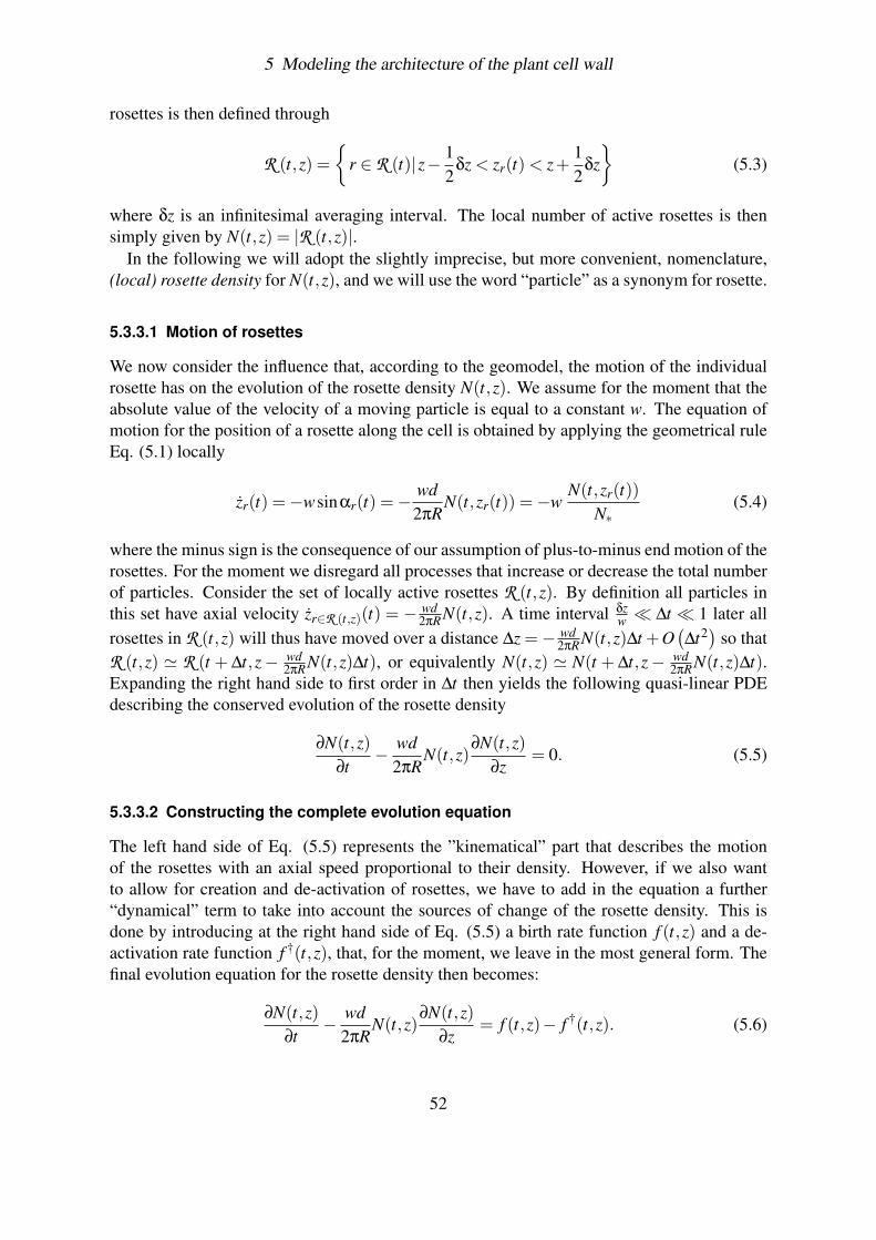
5 Modeling the architecture of the plant cell wall
rosettes is then defined through
R (t,z) =
r ∈ R (t)|z− 12
δz < zr(t) < z+12
δz
(5.3)
where δz is an infinitesimal averaging interval. The local number of active rosettes is thensimply given by N(t,z) = |R (t,z)|.
In the following we will adopt the slightly imprecise, but more convenient, nomenclature,(local) rosette density for N(t,z), and we will use the word “particle” as a synonym for rosette.
5.3.3.1 Motion of rosettes
We now consider the influence that, according to the geomodel, the motion of the individualrosette has on the evolution of the rosette density N(t,z). We assume for the moment that theabsolute value of the velocity of a moving particle is equal to a constant w. The equation ofmotion for the position of a rosette along the cell is obtained by applying the geometrical ruleEq. (5.1) locally
zr(t) =−wsinαr(t) =− wd2πR
N(t,zr(t)) =−wN(t,zr(t))
N∗(5.4)
where the minus sign is the consequence of our assumption of plus-to-minus end motion of therosettes. For the moment we disregard all processes that increase or decrease the total numberof particles. Consider the set of locally active rosettes R (t,z). By definition all particles inthis set have axial velocity zr∈R (t,z)(t) = − wd
2πRN(t,z). A time interval δzw ∆t 1 later all
rosettes in R (t,z) will thus have moved over a distance ∆z =− wd2πRN(t,z)∆t +O
(∆t2) so that
R (t,z) ' R (t + ∆t,z− wd2πRN(t,z)∆t), or equivalently N(t,z) ' N(t + ∆t,z− wd
2πRN(t,z)∆t).Expanding the right hand side to first order in ∆t then yields the following quasi-linear PDEdescribing the conserved evolution of the rosette density
∂N(t,z)∂t
− wd2πR
N(t,z)∂N(t,z)
∂z= 0. (5.5)
5.3.3.2 Constructing the complete evolution equation
The left hand side of Eq. (5.5) represents the ”kinematical” part that describes the motionof the rosettes with an axial speed proportional to their density. However, if we also wantto allow for creation and de-activation of rosettes, we have to add in the equation a further“dynamical” term to take into account the sources of change of the rosette density. This isdone by introducing at the right hand side of Eq. (5.5) a birth rate function f (t,z) and a de-activation rate function f †(t,z), that, for the moment, we leave in the most general form. Thefinal evolution equation for the rosette density then becomes:
∂N(t,z)∂t
− wd2πR
N(t,z)∂N(t,z)
∂z= f (t,z)− f †(t,z). (5.6)
52
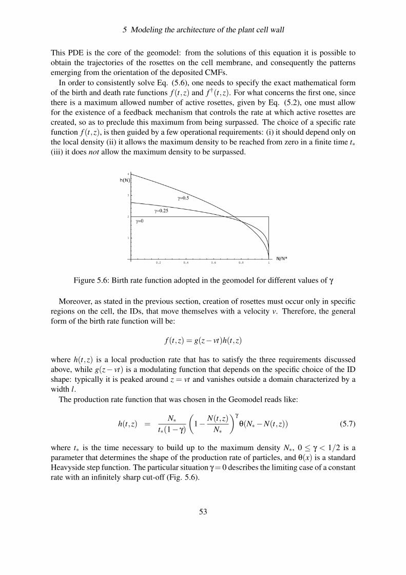
5 Modeling the architecture of the plant cell wall
This PDE is the core of the geomodel: from the solutions of this equation it is possible toobtain the trajectories of the rosettes on the cell membrane, and consequently the patternsemerging from the orientation of the deposited CMFs.
In order to consistently solve Eq. (5.6), one needs to specify the exact mathematical formof the birth and death rate functions f (t,z) and f †(t,z). For what concerns the first one, sincethere is a maximum allowed number of active rosettes, given by Eq. (5.2), one must allowfor the existence of a feedback mechanism that controls the rate at which active rosettes arecreated, so as to preclude this maximum from being surpassed. The choice of a specific ratefunction f (t,z), is then guided by a few operational requirements: (i) it should depend only onthe local density (ii) it allows the maximum density to be reached from zero in a finite time t∗(iii) it does not allow the maximum density to be surpassed.
Figure 5.6: Birth rate function adopted in the geomodel for different values of γ
Moreover, as stated in the previous section, creation of rosettes must occur only in specificregions on the cell, the IDs, that move themselves with a velocity v. Therefore, the generalform of the birth rate function will be:
f (t,z) = g(z− vt)h(t,z)
where h(t,z) is a local production rate that has to satisfy the three requirements discussedabove, while g(z− vt) is a modulating function that depends on the specific choice of the IDshape: typically it is peaked around z = vt and vanishes outside a domain characterized by awidth l.
The production rate function that was chosen in the Geomodel reads like:
h(t,z) =N∗
t∗(1− γ)
(1− N(t,z)
N∗
)γ
θ(N∗−N(t,z)) (5.7)
where t∗ is the time necessary to build up to the maximum density N∗, 0 ≤ γ < 1/2 is aparameter that determines the shape of the production rate of particles, and θ(x) is a standardHeavyside step function. The particular situation γ = 0 describes the limiting case of a constantrate with an infinitely sharp cut-off (Fig. 5.6).
53
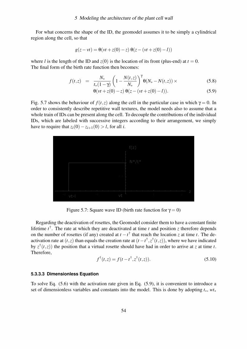
5 Modeling the architecture of the plant cell wall
For what concerns the shape of the ID, the geomodel assumes it to be simply a cylindricalregion along the cell, so that
g(z− vt) = θ(vt + z(0)− z) θ(z− (vt + z(0)− l))
where l is the length of the ID and z(0) is the location of its front (plus-end) at t = 0.The final form of the birth rate function then becomes:
f (t,z) =N∗
t∗(1− γ)
(1− N(t,z)
N∗
)γ
θ(N∗−N(t,z))× (5.8)
θ(vt + z(0)− z) θ(z− (vt + z(0)− l)). (5.9)
Fig. 5.7 shows the behaviour of f (t,z) along the cell in the particular case in which γ = 0. Inorder to consistently describe repetitive wall textures, the model needs also to assume that awhole train of IDs can be present along the cell. To decouple the contributions of the individualIDs, which are labeled with successive integers according to their arrangement, we simplyhave to require that zi(0)− zi+1(0) > l, for all i.
Figure 5.7: Square wave ID (birth rate function for γ = 0)
Regarding the deactivation of rosettes, the Geomodel consider them to have a constant finitelifetime t†. The rate at which they are deactivated at time t and position z therefore dependson the number of rosettes (if any) created at t− t† that reach the location z at time t. The de-activation rate at (t,z) than equals the creation rate at (t− t†,z†(t,z)), where we have indicatedby z†(t,z)) the position that a virtual rosette should have had in order to arrive at z at time t.Therefore,
f †(t,z) = f (t− t†,z†(t,z)). (5.10)
5.3.3.3 Dimensionless Equation
To solve Eq. (5.6) with the activation rate given in Eq. (5.9), it is convenient to introduce aset of dimensionless variables and constants into the model. This is done by adopting t∗, wt∗
54
5 Modeling the architecture of the plant cell wall
and N∗ as our units of time, length and density respectively. We are left then with the reducedindependent time, space and density variables
τ =tt∗
ζ =z
wt∗ν =
NN∗
. (5.11)
The dimensionless parameters of the model are therefore
λ = l/(wt∗) β = v/w τ† = t†/t∗ (5.12)
and the evolution equation (5.6) becomes
∂ν(τ,ζ)∂τ
−ν(τ,ζ)∂ν(τ,ζ)
∂ζ= φ(τ,ζ)−φ
†(τ,ζ) (5.13)
where
φ(τ,ζ) =(1−ν(τ,ζ))γ
1− γΘ(1−ν(τ,ζ))Θ(βτ−ζ)Θ(ζ− (βτ−λ)) (5.14)
andφ
†(τ,ζ) = φ(τ− τ†,ζ†(τ,ζ)).
We will return to the problem of self consistently determining ζ†(τ,ζ)) when we construct thesolutions of the evolution equation using the method of characteristics.
5.3.3.4 Method of solution
In order to solve Eq. (5.13) we apply the method of characteristics. The details of this methodof solution are reported in Appendix. Since we wish to study the solutions of the evolutionequation in absence of any transient or boundary related effects, we assume that cell walldeposition has started sufficiently long ago that all transient effects have died down: we areessentially in a steady state in which IDs from a long train are passing the origin (middle ofthe cell) at regular intervals. The zero of our timescale is now arbitrarily chosen such that atτ = 0, the front of a new ID is located at ζ = 0. The rosettes created in this ID will for τ > 0start spinning CMFs that will contribute to a new lamella being deposited in the regime ζ > 0.
The equations for the characteristics, which are parametrized by the variable s and identifiedby the initial value parameter p, follow directly from Eq. (5.13)
dτ(s; p)ds
= 1 (5.15)
dζ(s; p)ds
= −ν(s; p) (5.16)
dν(s; p)ds
= φ(s; p)−φ†(s; p) (5.17)
with initial conditions
τ(0; p) = 0 (5.18)ζ(0; p) = p (5.19)ν(0, p) = 0. (5.20)
55
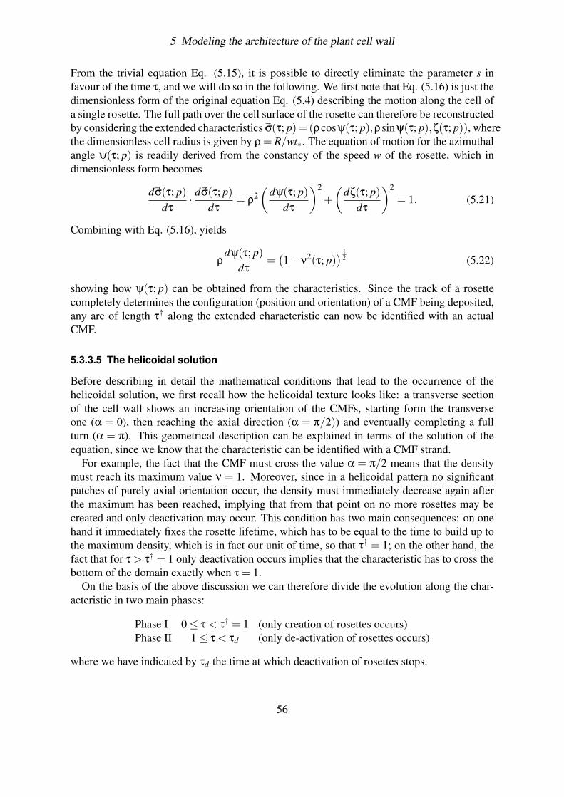
5 Modeling the architecture of the plant cell wall
From the trivial equation Eq. (5.15), it is possible to directly eliminate the parameter s infavour of the time τ, and we will do so in the following. We first note that Eq. (5.16) is just thedimensionless form of the original equation Eq. (5.4) describing the motion along the cell ofa single rosette. The full path over the cell surface of the rosette can therefore be reconstructedby considering the extended characteristics~σ(τ; p)= (ρcosψ(τ; p),ρsinψ(τ; p),ζ(τ; p)), wherethe dimensionless cell radius is given by ρ = R/wt∗. The equation of motion for the azimuthalangle ψ(τ; p) is readily derived from the constancy of the speed w of the rosette, which indimensionless form becomes
d~σ(τ; p)dτ
· d~σ(τ; p)dτ
= ρ2(
dψ(τ; p)dτ
)2
+(
dζ(τ; p)dτ
)2
= 1. (5.21)
Combining with Eq. (5.16), yields
ρdψ(τ; p)
dτ=(1−ν
2(τ; p)) 1
2 (5.22)
showing how ψ(τ; p) can be obtained from the characteristics. Since the track of a rosettecompletely determines the configuration (position and orientation) of a CMF being deposited,any arc of length τ† along the extended characteristic can now be identified with an actualCMF.
5.3.3.5 The helicoidal solution
Before describing in detail the mathematical conditions that lead to the occurrence of thehelicoidal solution, we first recall how the helicoidal texture looks like: a transverse sectionof the cell wall shows an increasing orientation of the CMFs, starting form the transverseone (α = 0), then reaching the axial direction (α = π/2)) and eventually completing a fullturn (α = π). This geometrical description can be explained in terms of the solution of theequation, since we know that the characteristic can be identified with a CMF strand.
For example, the fact that the CMF must cross the value α = π/2 means that the densitymust reach its maximum value ν = 1. Moreover, since in a helicoidal pattern no significantpatches of purely axial orientation occur, the density must immediately decrease again afterthe maximum has been reached, implying that from that point on no more rosettes may becreated and only deactivation may occur. This condition has two main consequences: on onehand it immediately fixes the rosette lifetime, which has to be equal to the time to build up tothe maximum density, which is in fact our unit of time, so that τ† = 1; on the other hand, thefact that for τ > τ† = 1 only deactivation occurs implies that the characteristic has to cross thebottom of the domain exactly when τ = 1.
On the basis of the above discussion we can therefore divide the evolution along the char-acteristic in two main phases:
Phase I 0≤ τ < τ† = 1 (only creation of rosettes occurs)Phase II 1≤ τ < τd (only de-activation of rosettes occurs)
where we have indicated by τd the time at which deactivation of rosettes stops.
56
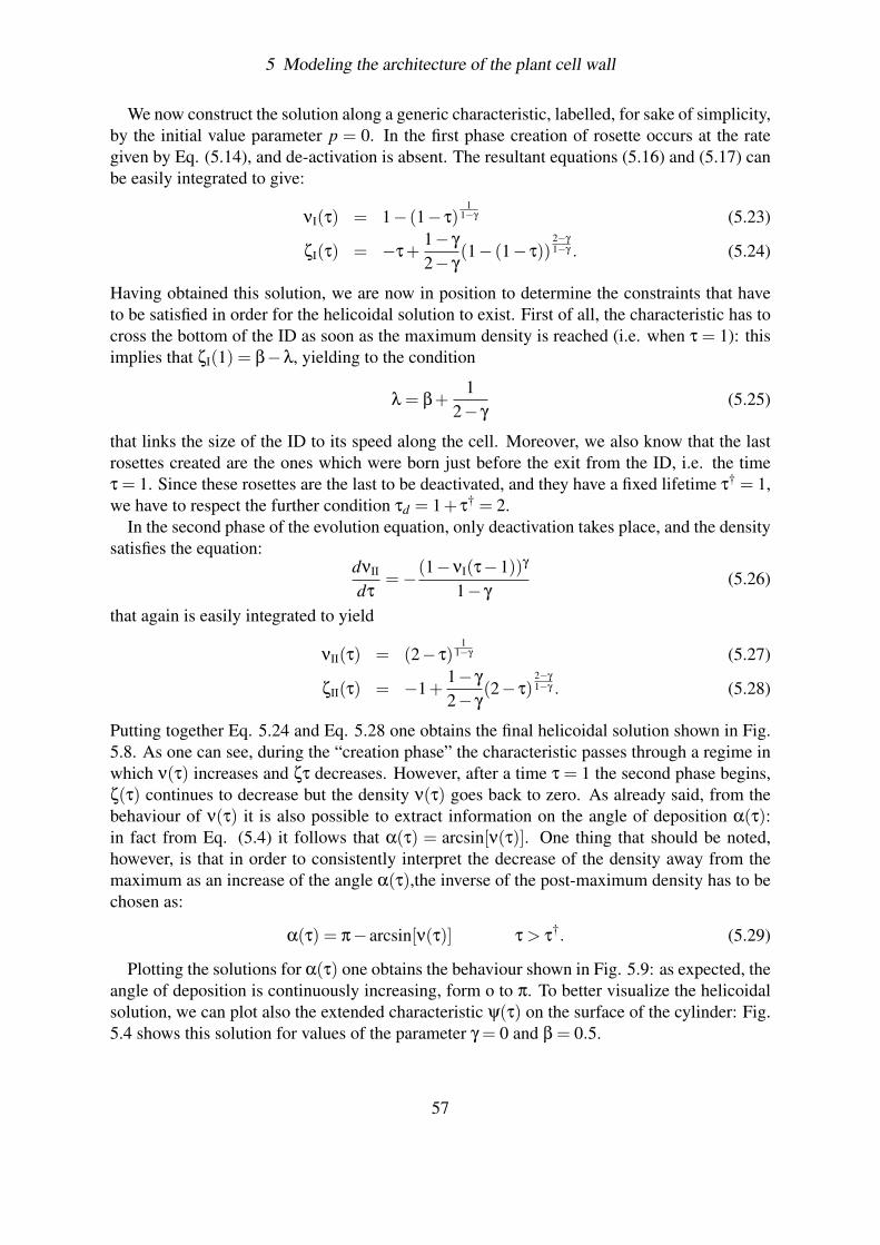
5 Modeling the architecture of the plant cell wall
We now construct the solution along a generic characteristic, labelled, for sake of simplicity,by the initial value parameter p = 0. In the first phase creation of rosette occurs at the rategiven by Eq. (5.14), and de-activation is absent. The resultant equations (5.16) and (5.17) canbe easily integrated to give:
νI(τ) = 1− (1− τ)1
1−γ (5.23)
ζI(τ) = −τ+1− γ
2− γ(1− (1− τ))
2−γ
1−γ . (5.24)
Having obtained this solution, we are now in position to determine the constraints that haveto be satisfied in order for the helicoidal solution to exist. First of all, the characteristic has tocross the bottom of the ID as soon as the maximum density is reached (i.e. when τ = 1): thisimplies that ζI(1) = β−λ, yielding to the condition
λ = β+1
2− γ(5.25)
that links the size of the ID to its speed along the cell. Moreover, we also know that the lastrosettes created are the ones which were born just before the exit from the ID, i.e. the timeτ = 1. Since these rosettes are the last to be deactivated, and they have a fixed lifetime τ† = 1,we have to respect the further condition τd = 1+ τ† = 2.
In the second phase of the evolution equation, only deactivation takes place, and the densitysatisfies the equation:
dνII
dτ=−(1−νI(τ−1))γ
1− γ(5.26)
that again is easily integrated to yield
νII(τ) = (2− τ)1
1−γ (5.27)
ζII(τ) = −1+1− γ
2− γ(2− τ)
2−γ
1−γ . (5.28)
Putting together Eq. 5.24 and Eq. 5.28 one obtains the final helicoidal solution shown in Fig.5.8. As one can see, during the “creation phase” the characteristic passes through a regime inwhich ν(τ) increases and ζτ decreases. However, after a time τ = 1 the second phase begins,ζ(τ) continues to decrease but the density ν(τ) goes back to zero. As already said, from thebehaviour of ν(τ) it is also possible to extract information on the angle of deposition α(τ):in fact from Eq. (5.4) it follows that α(τ) = arcsin[ν(τ)]. One thing that should be noted,however, is that in order to consistently interpret the decrease of the density away from themaximum as an increase of the angle α(τ),the inverse of the post-maximum density has to bechosen as:
α(τ) = π− arcsin[ν(τ)] τ > τ†. (5.29)
Plotting the solutions for α(τ) one obtains the behaviour shown in Fig. 5.9: as expected, theangle of deposition is continuously increasing, form o to π. To better visualize the helicoidalsolution, we can plot also the extended characteristic ψ(τ) on the surface of the cylinder: Fig.5.4 shows this solution for values of the parameter γ = 0 and β = 0.5.
57
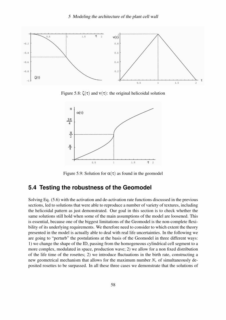
5 Modeling the architecture of the plant cell wall
Figure 5.8: ζ(τ) and ν(τ): the original helicoidal solution
Figure 5.9: Solution for α(τ) as found in the geomodel
5.4 Testing the robustness of the Geomodel
Solving Eq. (5.6) with the activation and de-activation rate functions discussed in the previoussections, led to solutions that were able to reproduce a number of variety of textures, includingthe helicoidal pattern as just demonstrated. Our goal in this section is to check whether thesame solutions still hold when some of the main assumptions of the model are loosened. Thisis essential, because one of the biggest limitations of the Geomodel is the non-complete flexi-bility of its underlying requirements. We therefore need to consider to which extent the theorypresented in the model is actually able to deal with real life uncertainties. In the following weare going to “perturb” the postulations at the basis of the Geomodel in three different ways:1) we change the shape of the ID, passing from the homogeneous cylindrical cell segment to amore complex, modulated in space, production wave; 2) we allow for a non fixed distributionof the life time of the rosettes; 2) we introduce fluctuations in the birth rate, constructing anew geometrical mechanism that allows for the maximum number N∗ of simultaneously de-posited rosettes to be surpassed. In all these three cases we demonstrate that the solutions of
58
5 Modeling the architecture of the plant cell wall
the geomodel are still stable and that the helicoidal pattern can be obtained as well.
5.4.1 The Triangular birth rate function
We start analyzing the effect that a spatially inhomogeneous birth rate has on the solutions ofthe Geomodel. Consider a constant production rate
h(t,z) =f∗l
Θ(N∗−N(t,z)) (5.30)
associated with a triangular modulating function
g(z− vt) = (vt− z)Θ(vt− z) Θ(z+ l− vt)+(z− vt +2l)Θ(vt− l− z) Θ(z− vt +2l).
The final birth rate function then becomes:
f (t,z) =
f∗l (vt− z) Θ(N∗−N(t,z)) if vt− l < z < vt,f∗l (z− vt +2l) Θ(N∗−N(t,z)) if vt−2l < z < vt− l.
and its behaviour is depicted schematically in Fig. 5.10. Here the ID has a total length 2l andtravels towards the cell plus end with a constant velocity v. The rosettes have a finite life-timet† and their rate of creation is not uniform along the domain but reaches its maximum valuef ∗ whenever z = vt− l (provided of course that N(t,z) < N∗).
Figure 5.10: Triangular local rate of production
In order solve Eq. (5.6) with this new activation rate, we again non-dimensionalize adoptingt∗ = N∗/ f∗, wt∗ and N∗ as our units of time, length and density respectively. With these newparameter the shape of the birth rate is described by the function
φ(τ,ζ) =
1λ
(βτ−ζ) Θ(1−ν(τ,ζ)) if βτ−λ < ζ < βτ,1λ
(ζ−βτ+2λ) Θ(1−ν(τ,ζ)) if βτ−2λ < ζ < βτ−λ.
where againφ
†(τ,ζ) = φ(τ− τ†,ζ†(τ,ζ)).
59

5 Modeling the architecture of the plant cell wall
5.4.1.1 Helicoidal texture
We start studying the solution along a characteristic labelled by the initial value parameter p =0. For the considerations carried out previously, we know that in order to have the helicoidalsolution, deactivation of rosettes has to begin exactly when creation stops, because the angleof deposition α has to decrease as soon as its maximum value π/2 is reached. This implies thatthe maximum number of active rosettes must be reached as soon as the characteristic crossesthe bottom of the ID. The evolution along the characteristic can be divided in four phases:
Phase I 0≤ τ < τ1 (passage of first region of triangular domain - negative slope)Phase II τ1 ≤ τ < τ2 (passage of second region triangular domain - positive slope)Phase III τ2 ≤ τ < τ1 + τ2 (death of rosette born during Phase I)Phase IV τ1 + τ2 ≤ τ < 2τ2 (death of rosette born during Phase II)
Phase I and II: In the first phase creation of rosettes is due to the passage of the first regionof the triangular domain, and deactivation is absent. The governing equations are therefore:
dζI
dτ= −νI(τ) (5.31)
dνI
dτ=
1λ(βτ−ζI(τ)) (5.32)
with initial conditions
ζI(0) = 0 (5.33)νI(0) = 0. (5.34)
The above system is easily integrated and gives
ζI(τ) = β
(τ−
√λ sinh
[τ√λ
])(5.35)
This solution is valid until a time τ1 =√
λ asinh[√
λ
β
], where the variable τ1 satisfies the
condition ζI(τ1) = βτ1−λ. At this time, in fact, the characteristic ζI(τ) crosses the region ofthe triangular domain with a negative slope. In this second phase deactivation is still absent,and the equations read like:
dζII
dτ= −νII(τ) (5.36)
dνII
dτ=
1λ(2λ−βτ+ζII(τ)) (5.37)
with initial conditions:
ζII(τ1) = ζI(τ1) (5.38)νII(τ1) = νI(τ1). (5.39)
60
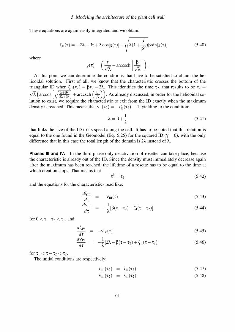
5 Modeling the architecture of the plant cell wall
These equations are again easily integrated and we obtain:
ζII(τ) =−2λ+βτ+λcos[g(τ)]−
√λ(1+
λ
β2 )βsin[g(τ)] (5.40)
where
g(τ) =(
τ√λ− arccsch
[β√λ
]).
At this point we can determine the conditions that have to be satisfied to obtain the he-licoidal solution. First of all, we know that the characteristic crosses the bottom of thetriangular ID when ζII(τ2) = βτ2 − 2λ. This identifies the time τ2, that results to be τ2 =√
λ
(arccos
[√λ+β2
2λ+β2
]+ arccsch
(β√λ
)). As already discussed, in order for the helicoidal so-
lution to exist, we require the characteristic to exit from the ID exactly when the maximumdensity is reached. This means that νII(τ2) =−ζ′II(τ2)≡ 1, yielding to the condition:
λ = β+12
(5.41)
that links the size of the ID to its speed along the cell. It has to be noted that this relation isequal to the one found in the Geomodel (Eq. 5.25) for the squared ID (γ = 0), with the onlydifference that in this case the total length of the domain is 2λ instead of λ.
Phases III and IV: In the third phase only deactivation of rosettes can take place, becausethe characteristic is already out of the ID. Since the density must immediately decrease againafter the maximum has been reached, the lifetime of a rosette has to be equal to the time atwhich creation stops. That means that
τ† = τ2 (5.42)
and the equations for the characteristics read like:
dζIII
dτ= −νIII(τ) (5.43)
dνIII
dτ= −1
λ[β(τ− τ2)−ζI(τ− τ2)] (5.44)
for 0 < τ− τ2 < τ1, and:
dζIV
dτ= −νIV(τ) (5.45)
dνIV
dτ= −1
λ[2λ−β(τ− τ2)+ζII(τ− τ2)] (5.46)
for τ1 < τ− τ2 < τ2.The initial conditions are respectively:
ζIII(τ2) = ζII(τ2) (5.47)νIII(τ2) = νII(τ2) (5.48)
61
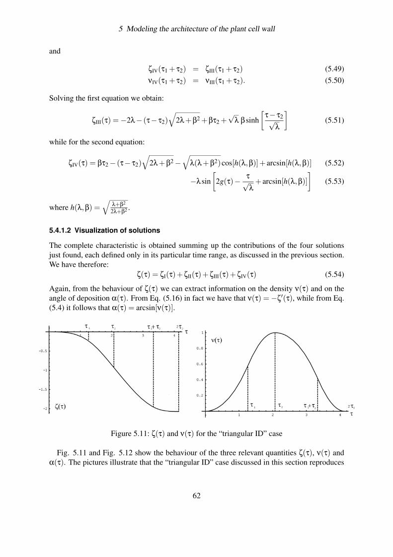
5 Modeling the architecture of the plant cell wall
and
ζIV(τ1 + τ2) = ζIII(τ1 + τ2) (5.49)νIV(τ1 + τ2) = νIII(τ1 + τ2). (5.50)
Solving the first equation we obtain:
ζIII(τ) =−2λ− (τ− τ2)√
2λ+β2 +βτ2 +√
λ βsinh[
τ− τ2√λ
](5.51)
while for the second equation:
ζIV(τ) = βτ2− (τ− τ2)√
2λ+β2−√
λ(λ+β2)cos[h(λ,β)]+ arcsin[h(λ,β)] (5.52)
−λsin[
2g(τ)− τ√λ
+ arcsin[h(λ,β)]]
(5.53)
where h(λ,β) =√
λ+β2
2λ+β2 .
5.4.1.2 Visualization of solutions
The complete characteristic is obtained summing up the contributions of the four solutionsjust found, each defined only in its particular time range, as discussed in the previous section.We have therefore:
ζ(τ) = ζI(τ)+ζII(τ)+ζIII(τ)+ζIV(τ) (5.54)
Again, from the behaviour of ζ(τ) we can extract information on the density ν(τ) and on theangle of deposition α(τ). From Eq. (5.16) in fact we have that ν(τ) =−ζ′(τ), while from Eq.(5.4) it follows that α(τ) = arcsin[ν(τ)].
Figure 5.11: ζ(τ) and ν(τ) for the “triangular ID” case
Fig. 5.11 and Fig. 5.12 show the behaviour of the three relevant quantities ζ(τ), ν(τ) andα(τ). The pictures illustrate that the “triangular ID” case discussed in this section reproduces
62
5 Modeling the architecture of the plant cell wall
well the helicoidal solution examined in the Geomodel: once assumed the post maximumsolution to be
α(τ) = π− arcsin[ν(τ)] τ > τ2.
we have that the angle of deposition α(t) in fact is continuously increasing until the valueα = π.
Figure 5.12: α(t) for the “triangular ID” case
5.4.2 Aging
The next step to test the robustness of the geomodel is to allow for a non-constant life timeof the rosettes. In order to do this, we need to introduce the concept of “age”: let thereforen(µ;z, t)dµ denote the number of synthases of age µ per unit length at position z at time t.From this definition it follows that
N (z, t) =Z
∞
0dµ n(µ;z, t) (5.55)
is the total number of synthases per unit length at position z and time t. Our goal in this sectionis to build up a structured population version of the evolution equation for the rosette densityand to resume the same solutions already found in the Geomodel.
5.4.2.1 The evolution equation
We begin recovering Eq. (5.5) starting from the dynamics of this new variable. In the absenceof “birth” and “death” processes the equation of motion for n(µ;z, t) can be derived as follows:in a small time interval dt the sub population n(µ;z, t) ages by dt and moves down the cellover a distance dz =− wd
2πRN (z, t)dt, as already discussed in section 5.3.3.1. Hence
n(
µ+dt;z− wd2πR
N (z, t)dt, t +dt)
= n(µ;z, t) . (5.56)
63
5 Modeling the architecture of the plant cell wall
Expanding the left hand side then yields
∂n(µ;z, t)∂µ
− wd2πR
N (z, t)∂n(µ;z, t)
∂z+
∂n(µ;z, t)∂t
= 0 (5.57)
and integrating over µ leads us to Eq. (5.5):
− wd2πR
N (z, t)∂N (z, t)
∂z+
∂N (z, t)∂t
= 0 (5.58)
were we have used the fact that n(0;z, t) = 0 as no new synthases are produced (the birth rateis zero) and n(∞;z, t) = 0 for finite t.
We now turn to the problem of determining the spatio-temporal evolution equation forn(µ; t,z). Consider for the moment non-moving synthases (w = 0), and new synthase pro-duction occurring at a fixed location z0 by a function f (N (t,z0)). For µ > 0 we have
n(µ+dt; t +dt,z0) = n(µ; t,z0) (5.59)
so that∂n(µ; t,z0)
∂µ+
∂n(µ; t,z0)∂t
= 0 (5.60)
which is solved by an arbitrary function n(µ; t,z0) = n(t−µ,z0) . Now consider what happensfor µ = 0: the number of rosettes of age µ = 0 in z0 is equal, by definition, to the number ofrosettes created in z0 by the local rate of production f (N(t)). This implies that:
n(0; t,z0) = f (N (t,z0)) = n(t,z0) (5.61)
and hencen(µ; t,z0) = f (N (t−µ,z0)) (5.62)
We now generalize to the case in which new synthase production takes place not only at afixed location z0, but within an insertion domain (ID), that in itself moves with a velocity v.The local rate of production is then described by a function
n(0;z, t) = F (z, t,N(z, t)) = g(z− vt) f (N (z, t)) (5.63)
where, as said in the previous section, g(z) depends upon the specific choice of the ID shape.Finally, we turn to the “de-activation” processes. With the definition of the new variable
n(µ; t,z), it is now possible to allow for death rates that depend on the age µ of the rosettes.We assume, therefore, that synthases are deactivated at a generic rate r (µ). The full equationbecomes
∂n(µ;z, t)∂µ
− wd2πR
N (z, t)∂n(µ;z, t)
∂z+
∂n(µ;z, t)∂t
=−r (µ)n(µ;z, t) (5.64)
n(0;z, t) = F (z, t,N (z, t)) . (5.65)
Looking at this equation it is possible to note that, differently from what we have seen in theprevious section, the birth rate function n(0;z, t) doesn’t appear anymore in the right handside of the evolution equation. Rather, it plays the role of a boundary condition that has to bespecified to consistently solve the equation. We will return to this point in the next section.
64

5 Modeling the architecture of the plant cell wall
5.4.2.2 Example: the Poissonian Decay
To better elucidate the meaning of the new evolution equation, we start focusing our attentionon a quite simple example. Let r (µ) be a Poissonian decay rate, i.e. r (µ) = −µ−1
† . Here µ†is a constant that represents the average time after which the number of rosettes significantlydecreases, independently from the specific age of the particles. We are going to couple thisdecay process with the standard “square wave” ID and constant production rate (Eq. 5.9), sothat the full equation becomes
∂n(µ;z, t)∂µ
− wd2πR
N (z, t)∂n(µ;z, t)
∂z+
∂n(µ;z, t)∂t
=− 1µ†
n(µ;z, t) (5.66)
n(0;z, t) =N∗
t∗θ(vt− z)θ(l− (vt− z))θ(N∗−N (z, t)) (5.67)
where t∗ is the time necessary to build up to the maximum density. As the death rate does notdepend on age we can integrate over µ to obtain
∂N (z, t)∂t
− wd2πR
N (z, t)∂N (z, t)
∂z= f∗θ(vt− z)θ(l− (vt− z))θ(N∗−N (z, t))− 1
µ†N (z, t)
(5.68)so that we are back to the evolution equation for our original variable N(t,z): as one can see,this equation is just a specific case of Eq. (5.6) with a non-constant life time of the rosettes. Ifwe non-dimensionalize by setting
τ =tt∗
ζ =z
wt∗ν =
NN∗
we then obtain the final equation
∂ν(ζ,τ)∂τ
−ν(ζ,τ)∂ν(ζ,τ)
∂ζ= θ(βτ−ζ)θ(λ− (βτ−ζ))θ(1−ν(ζ,τ))− 1
ϕ†ν(ζ,τ) (5.69)
whereβ =
vw
λ =l
wt∗ϕ† =
µ†
t∗.
We now follow the procedures described in Appendix to obtain the solution along a character-istic specified by the initial data
ζ(0; p) = p (5.70)ν(0; p) = 0. (5.71)
Along the characteristics we have the coupled equations
dζ(τ; p)dτ
=−ν(τ; p) (5.72)
dν(τ; p)dτ
= θ(βτ−ζ(τ; p))θ(λ− (βτ−ζ(τ; p)))θ(1−ν(τ; p))− 1ϕ†
ν(τ; p) . (5.73)
65
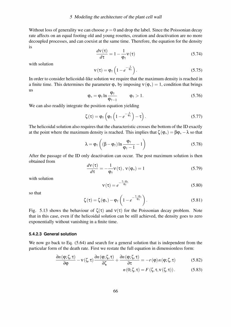
5 Modeling the architecture of the plant cell wall
Without loss of generality we can choose p = 0 and drop the label. Since the Poissonian decayrate affects on an equal footing old and young rosettes, creation and deactivation are no moredecoupled processes, and can coexist at the same time. Therefore, the equation for the densityis
dν(τ)dτ
= 1− 1ϕ†
ν(τ) (5.74)
with solutionν(τ) = ϕ†
(1− e
− τ
ϕ†
). (5.75)
In order to consider helicoidal-like solution we require that the maximum density is reached ina finite time. This determines the parameter ϕ∗ by imposing ν(ϕ∗) = 1, condition that bringsus
ϕ∗ = ϕ† lnϕ†
ϕ†−1ϕ† > 1. (5.76)
We can also readily integrate the position equation yielding
ζ(τ) = ϕ†
(ϕ†
(1− e
− τ
ϕ†
)− τ
). (5.77)
The helicoidal solution also requires that the characteristic crosses the bottom of the ID exactlyat the point where the maximum density is reached. This implies that ζ(ϕ∗) = βϕ∗−λ so that
λ = ϕ†
((β−ϕ†) ln
ϕ†
ϕ†−1−1)
(5.78)
After the passage of the ID only deactivation can occur. The post maximum solution is thenobtained from
dν(τ)dτ
=− 1ϕ†
ν(τ) , ν(ϕ∗) = 1 (5.79)
with solutionν(τ) = e
− τ−ϕ∗ϕ† (5.80)
so that
ζ(τ) = ζ(ϕ∗)−ϕ†
(1− e
− τ−ϕ∗ϕ†
). (5.81)
Fig. 5.13 shows the behaviour of ζ(τ) and ν(τ) for the Poissonian decay problem. Notethat in this case, even if the helicoidal solution can be still achieved, the density goes to zeroexponentially without vanishing in a finite time.
5.4.2.3 General solution
We now go back to Eq. (5.64) and search for a general solution that is independent from theparticular form of the death rate. First we restate the full equation in dimensionless form:
∂n(ϕ;ζ,τ)∂ϕ
−ν(ζ,τ)∂n(ϕ;ζ,τ)
∂ζ+
∂n(ϕ;ζ,τ)∂τ
=−r (ϕ)n(ϕ;ζ,τ) (5.82)
n(0;ζ,τ) = F (ζ,τ,ν(ζ,τ)) . (5.83)
66
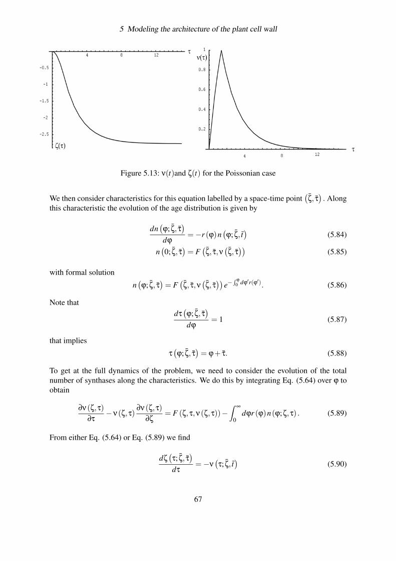
5 Modeling the architecture of the plant cell wall
Figure 5.13: ν(t)and ζ(t) for the Poissonian case
We then consider characteristics for this equation labelled by a space-time point(ζ, τ). Along
this characteristic the evolution of the age distribution is given by
dn(ϕ; ζ, τ
)dϕ
=−r (ϕ)n(ϕ; ζ, t
)(5.84)
n(0; ζ, τ
)= F
(ζ, τ,ν
(ζ, τ))
(5.85)
with formal solution
n(ϕ; ζ, τ
)= F
(ζ, τ,ν
(ζ, τ))
e−R ϕ
0 dϕ′r(ϕ′). (5.86)
Note thatdτ(ϕ; ζ, τ
)dϕ
= 1 (5.87)
that implies
τ(ϕ; ζ, τ
)= ϕ+ τ. (5.88)
To get at the full dynamics of the problem, we need to consider the evolution of the totalnumber of synthases along the characteristics. We do this by integrating Eq. (5.64) over ϕ toobtain
∂ν(ζ,τ)∂τ
−ν(ζ,τ)∂ν(ζ,τ)
∂ζ= F (ζ,τ,ν(ζ,τ))−
Z∞
0dϕr (ϕ)n(ϕ;ζ,τ) . (5.89)
From either Eq. (5.64) or Eq. (5.89) we find
dζ(τ; ζ, τ
)dτ
=−ν(τ; ζ, t
)(5.90)
67
5 Modeling the architecture of the plant cell wall
so that along the characteristic we have
dν(τ; ζ, τ
)dτ
= F(ζ(τ; ζ, τ
),τ,ν
(ζ(τ; ζ, τ
),τ))−
Z∞
0dϕr (ϕ)n
(ϕ;ζ
(τ−ϕ; ζ, τ
),τ−ϕ
)= F
(ζ(τ; ζ, τ
),τ,ν
(ζ(τ; ζ, τ
),τ))
−Z
∞
0dϕr (ϕ)F
(ζ(τ−ϕ; ζ, τ
),τ−ϕ,ν
(τ−ϕ; ζ, τ
))e−
R ϕ
0 dϕ′r(ϕ′) (5.91)
which is a functional delay equation.If
r (ϕ) =
0 0≤ ϕ < ϕ†∞ ϕ≥ ϕ†
(5.92)
then
dν(τ; ζ, τ
)dτ
= F(ζ(τ; ζ, τ
),τ,ν
(ζ(τ; ζ, τ
),τ))−F
(ζ(τ−ϕ†; ζ, τ
),τ−ϕ†,ν
(τ−ϕ; ζ, τ
))(5.93)
which is the original case considered in the geomodel.The second term on the right hand side of Eq. (5.91) can also be partially integrated to yield
dν(τ; ζ, τ
)dτ
=−Z
∞
0dϕe−
R ϕ
0 dϕ′r(ϕ′) ddϕ
F(ζ(τ−ϕ; ζ, τ
),τ−ϕ,ν
(τ−ϕ; ζ, τ
)). (5.94)
The latter form is especially convenient when F is of the “square wave” constant productionrate type. In this case the derivative dF
dϕthen is identically zero except at the switching points,
where it becomes a δ-function. Let us denote
R(ϕ) =Z
ϕ
0dϕ
′r(ϕ′) . (5.95)
and consider the characteristic starting from ζ = τ = 0. In the pre-maximum density phase,the solution must then obey
dν< (τ)dτ
=Z
∞
0dϕe−R(ϕ)
δ(τ−ϕ) = e−R(τ) (5.96)
ν< (0) = 0 (5.97)
with solution
ν< (τ) =Z
τ
0dϕe−R(ϕ). (5.98)
Let τ1 be the time at which the maximum density is reached, so that
ν< (τ1) =Z
τ1
0dϕe−R(ϕ) = 1. (5.99)
68
5 Modeling the architecture of the plant cell wall
Assume also that at τ1 the helicoidal condition is met, so that production is fully cut off. Thenthe post maximum equation is
dν> (τ)dτ
=−Z
∞
0dϕe−R(ϕ) −δ(τ−ϕ)+δ(τ−ϕ− τ1)= e−R(τ)− e−R(τ−τ1) (5.100)
ν> (τ1) = 1 (5.101)
with solution
ν> (τ) = 1+Z
τ
τ1
dϕ
e−R(ϕ)− e−R(ϕ−τ1)
. Inserting R(ϕ) = ϕ
ϕ†and τ1 = ϕ† ln ϕ†
ϕ†−1and some algebra retrieves the previously discussed
Poissonian case. Another special case is R(ϕ) = 0 for ϕ ≤ 1 and R(ϕ) = ∞ for ϕ > 1 (thehelicoidal γ = 0 case of the original model). Here we recover
ν< (τ) = τ (5.102)
andν> (τ) = 2− τ (5.103)
which essentially are the results Eqs. (5.23) and (5.27) presented before.
5.4.3 Effect of fluctuations
Another way to test the robustness of the Geomodel, is to verify the validity of its solutions inpresence of fluctuations of the birth rate of rosettes. From now on, we will then assume thatthe local production rate of particles is described by a function
G(t,z) = h(t,z)+η(t,z) (5.104)
where h(t,z) is a deterministic production rate, like for example the ones discussed in Eq.(5.7) or Eq. (5.30), and η(t,z) represents the effect of fluctuations that can locally increase ordecrease the number of created rosettes.
5.4.3.1 Solving the problem of overcrowding
To fully take into account the effect of this randomness on the trajectories of the rosettes, andtherefore on the orientation of the deposited CMFs, we need to slightly modify one of themain elements of the original Geomodel: we have to allow for the maximum local number N∗of particles to be surpassed. The main consequence of the presence of a noise term in the birthrate, in fact, is to provoke in some cases an overcrowding of the rosettes, whose number canthen increase beyond the maximum value N∗. The original geomodel would be inconsistentwith respect to such a perturbation: from Eq. (5.4) it is clear, in fact, that, if N(t,z) > N∗, theaxial speed z(t) of a particle would be greater than its present absolute velocity w.
69
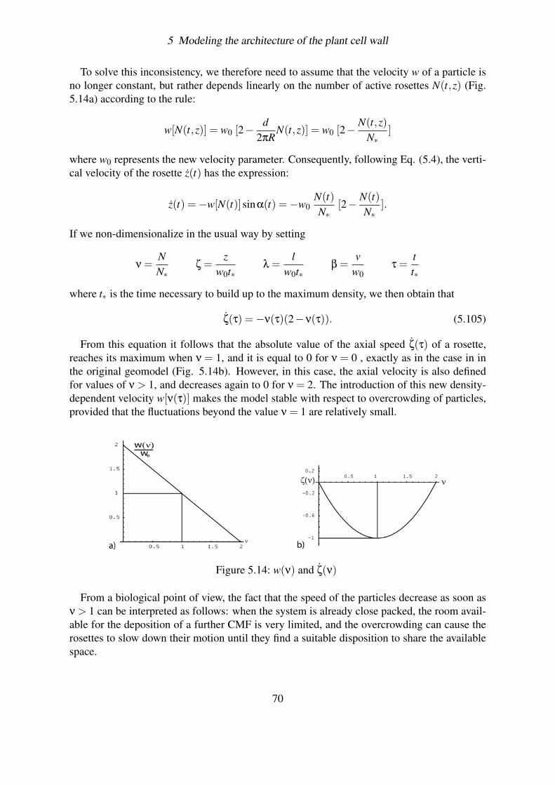
5 Modeling the architecture of the plant cell wall
To solve this inconsistency, we therefore need to assume that the velocity w of a particle isno longer constant, but rather depends linearly on the number of active rosettes N(t,z) (Fig.5.14a) according to the rule:
w[N(t,z)] = w0 [2− d2πR
N(t,z)] = w0 [2− N(t,z)N∗
]
where w0 represents the new velocity parameter. Consequently, following Eq. (5.4), the verti-cal velocity of the rosette z(t) has the expression:
z(t) =−w[N(t)]sinα(t) =−w0N(t)N∗
[2− N(t)N∗
].
If we non-dimensionalize in the usual way by setting
ν =NN∗
ζ =z
w0t∗λ =
lw0t∗
β =v
w0τ =
tt∗
where t∗ is the time necessary to build up to the maximum density, we then obtain that
ζ(τ) =−ν(τ)(2−ν(τ)). (5.105)
From this equation it follows that the absolute value of the axial speed ζ(τ) of a rosette,reaches its maximum when ν = 1, and it is equal to 0 for ν = 0 , exactly as in the case in inthe original geomodel (Fig. 5.14b). However, in this case, the axial velocity is also definedfor values of ν > 1, and decreases again to 0 for ν = 2. The introduction of this new density-dependent velocity w[ν(τ)] makes the model stable with respect to overcrowding of particles,provided that the fluctuations beyond the value ν = 1 are relatively small.
Figure 5.14: w(ν) and ζ(ν)
From a biological point of view, the fact that the speed of the particles decrease as soon asν > 1 can be interpreted as follows: when the system is already close packed, the room avail-able for the deposition of a further CMF is very limited, and the overcrowding can cause therosettes to slow down their motion until they find a suitable disposition to share the availablespace.
70
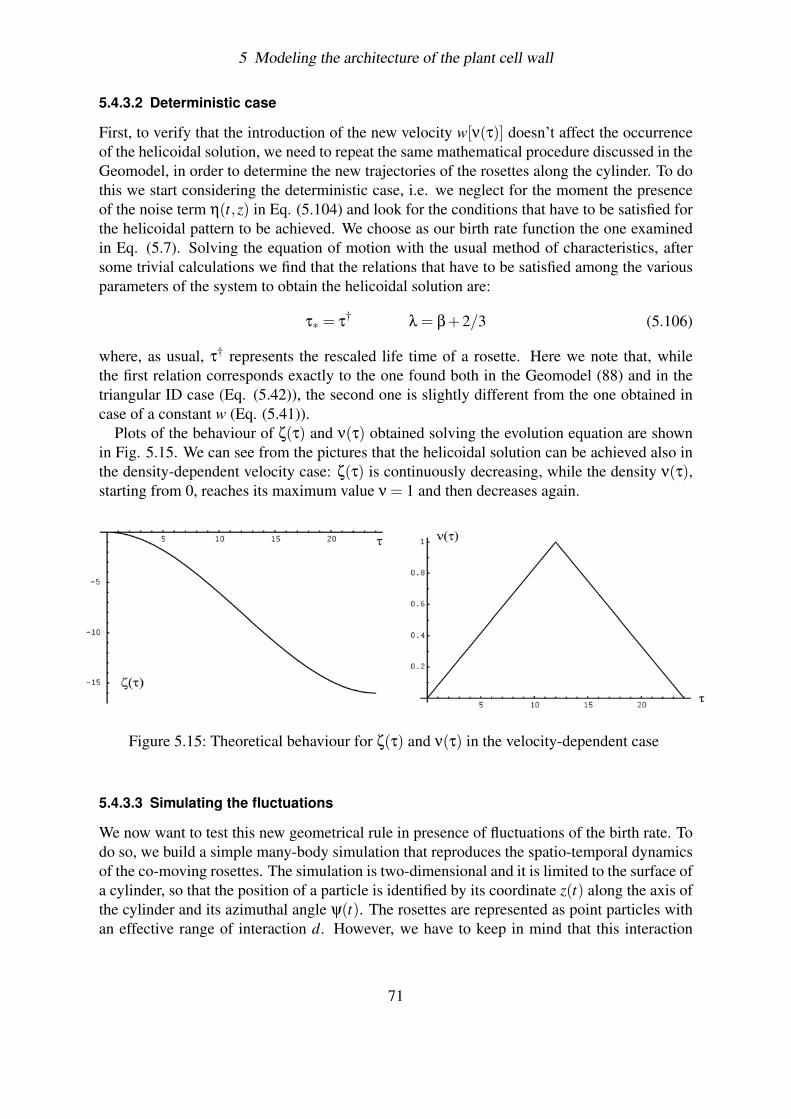
5 Modeling the architecture of the plant cell wall
5.4.3.2 Deterministic case
First, to verify that the introduction of the new velocity w[ν(τ)] doesn’t affect the occurrenceof the helicoidal solution, we need to repeat the same mathematical procedure discussed in theGeomodel, in order to determine the new trajectories of the rosettes along the cylinder. To dothis we start considering the deterministic case, i.e. we neglect for the moment the presenceof the noise term η(t,z) in Eq. (5.104) and look for the conditions that have to be satisfied forthe helicoidal pattern to be achieved. We choose as our birth rate function the one examinedin Eq. (5.7). Solving the equation of motion with the usual method of characteristics, aftersome trivial calculations we find that the relations that have to be satisfied among the variousparameters of the system to obtain the helicoidal solution are:
τ∗ = τ†
λ = β+2/3 (5.106)
where, as usual, τ† represents the rescaled life time of a rosette. Here we note that, whilethe first relation corresponds exactly to the one found both in the Geomodel (88) and in thetriangular ID case (Eq. (5.42)), the second one is slightly different from the one obtained incase of a constant w (Eq. (5.41)).
Plots of the behaviour of ζ(τ) and ν(τ) obtained solving the evolution equation are shownin Fig. 5.15. We can see from the pictures that the helicoidal solution can be achieved also inthe density-dependent velocity case: ζ(τ) is continuously decreasing, while the density ν(τ),starting from 0, reaches its maximum value ν = 1 and then decreases again.
Figure 5.15: Theoretical behaviour for ζ(τ) and ν(τ) in the velocity-dependent case
5.4.3.3 Simulating the fluctuations
We now want to test this new geometrical rule in presence of fluctuations of the birth rate. Todo so, we build a simple many-body simulation that reproduces the spatio-temporal dynamicsof the co-moving rosettes. The simulation is two-dimensional and it is limited to the surface ofa cylinder, so that the position of a particle is identified by its coordinate z(t) along the axis ofthe cylinder and its azimuthal angle ψ(t). The rosettes are represented as point particles withan effective range of interaction d. However, we have to keep in mind that this interaction
71
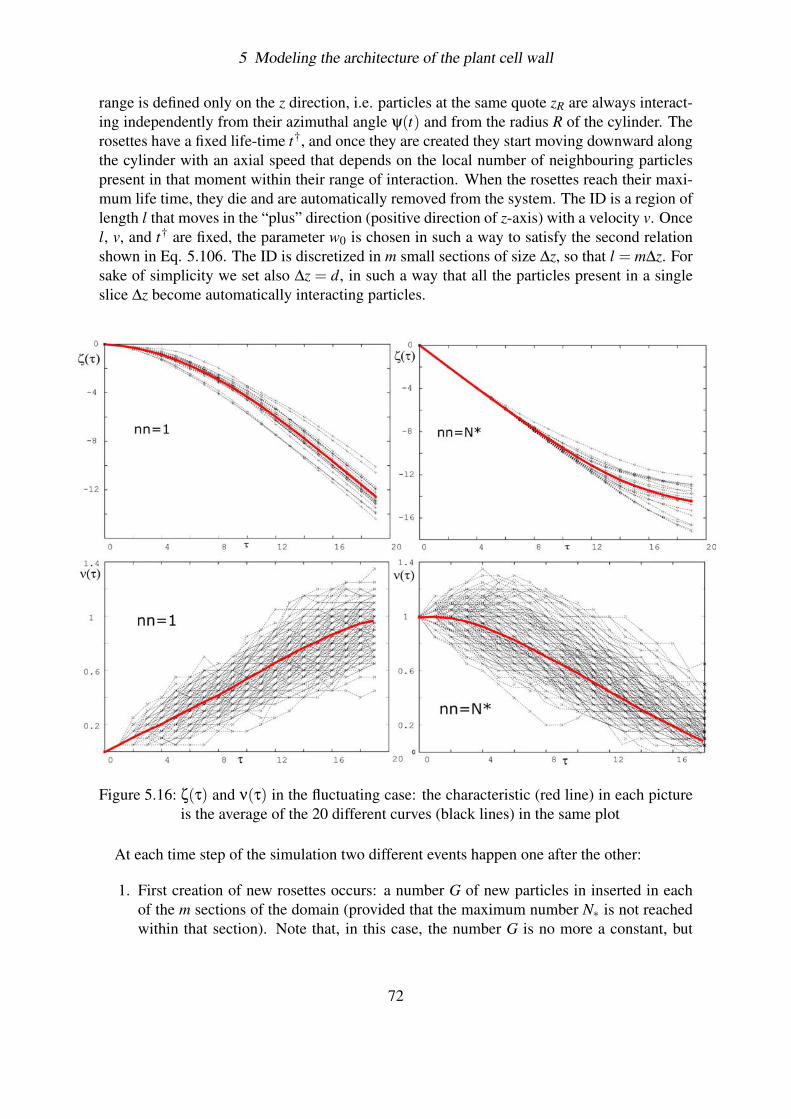
5 Modeling the architecture of the plant cell wall
range is defined only on the z direction, i.e. particles at the same quote zR are always interact-ing independently from their azimuthal angle ψ(t) and from the radius R of the cylinder. Therosettes have a fixed life-time t†, and once they are created they start moving downward alongthe cylinder with an axial speed that depends on the local number of neighbouring particlespresent in that moment within their range of interaction. When the rosettes reach their maxi-mum life time, they die and are automatically removed from the system. The ID is a region oflength l that moves in the “plus” direction (positive direction of z-axis) with a velocity v. Oncel, v, and t† are fixed, the parameter w0 is chosen in such a way to satisfy the second relationshown in Eq. 5.106. The ID is discretized in m small sections of size ∆z, so that l = m∆z. Forsake of simplicity we set also ∆z = d, in such a way that all the particles present in a singleslice ∆z become automatically interacting particles.
Figure 5.16: ζ(τ) and ν(τ) in the fluctuating case: the characteristic (red line) in each pictureis the average of the 20 different curves (black lines) in the same plot
At each time step of the simulation two different events happen one after the other:
1. First creation of new rosettes occurs: a number G of new particles in inserted in eachof the m sections of the domain (provided that the maximum number N∗ is not reachedwithin that section). Note that, in this case, the number G is no more a constant, but
72
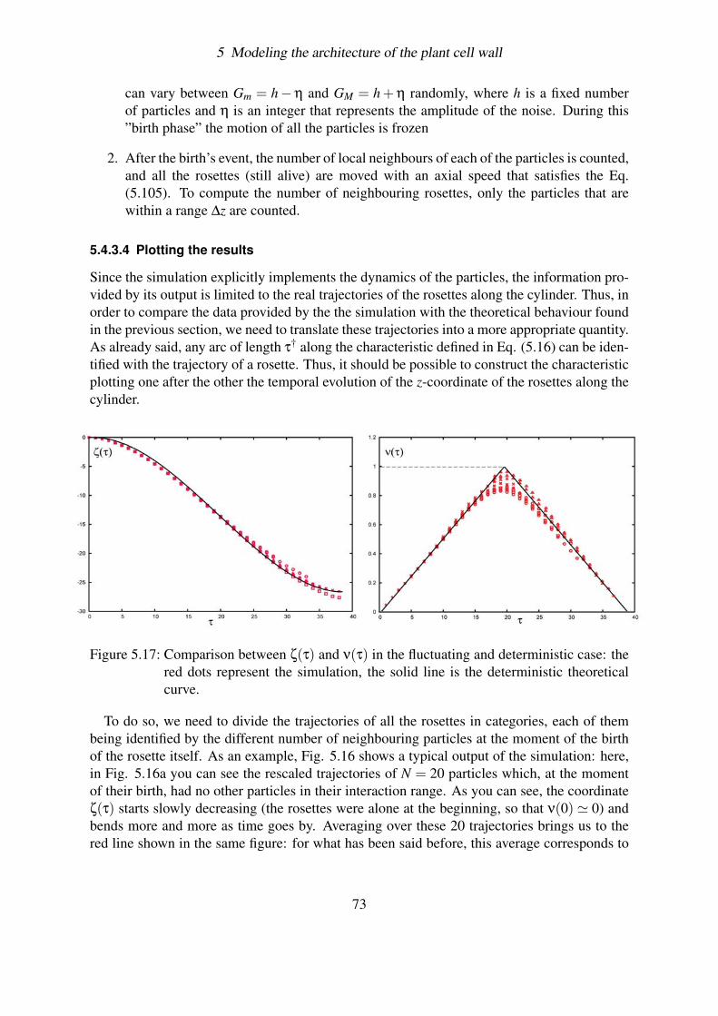
5 Modeling the architecture of the plant cell wall
can vary between Gm = h−η and GM = h + η randomly, where h is a fixed numberof particles and η is an integer that represents the amplitude of the noise. During this”birth phase” the motion of all the particles is frozen
2. After the birth’s event, the number of local neighbours of each of the particles is counted,and all the rosettes (still alive) are moved with an axial speed that satisfies the Eq.(5.105). To compute the number of neighbouring rosettes, only the particles that arewithin a range ∆z are counted.
5.4.3.4 Plotting the results
Since the simulation explicitly implements the dynamics of the particles, the information pro-vided by its output is limited to the real trajectories of the rosettes along the cylinder. Thus, inorder to compare the data provided by the the simulation with the theoretical behaviour foundin the previous section, we need to translate these trajectories into a more appropriate quantity.As already said, any arc of length τ† along the characteristic defined in Eq. (5.16) can be iden-tified with the trajectory of a rosette. Thus, it should be possible to construct the characteristicplotting one after the other the temporal evolution of the z-coordinate of the rosettes along thecylinder.
Figure 5.17: Comparison between ζ(τ) and ν(τ) in the fluctuating and deterministic case: thered dots represent the simulation, the solid line is the deterministic theoreticalcurve.
To do so, we need to divide the trajectories of all the rosettes in categories, each of thembeing identified by the different number of neighbouring particles at the moment of the birthof the rosette itself. As an example, Fig. 5.16 shows a typical output of the simulation: here,in Fig. 5.16a you can see the rescaled trajectories of N = 20 particles which, at the momentof their birth, had no other particles in their interaction range. As you can see, the coordinateζ(τ) starts slowly decreasing (the rosettes were alone at the beginning, so that ν(0) ' 0) andbends more and more as time goes by. Averaging over these 20 trajectories brings us to thered line shown in the same figure: for what has been said before, this average corresponds to
73
5 Modeling the architecture of the plant cell wall
the first part of the theoretical characteristic. Let’s now consider the case of rosettes that wereborn with a number N∗ of neighbouring particles in their interaction range. In this case, asyou can see from Fig. 5.16b ,the trajectories start very bent (the maximum number N∗ in factcorresponds to a value ν(0) = 1) and slowly decrease in time.
The same procedure can be applied for ν(τ): in this case, to plot the temporal behaviour ofthis quantity, it is sufficient to count the number of particles that a rosette encounters alongthis trajectory. As an example, Fig. 5.16c-d show the temporal evolution of the number ofparticles encountered by N = 20 different rosettes, in case in which they had 0 (Fig. 5.16c) orN∗ (Fig. 5.16d) neighbouring particles in their interaction range at the moment of their birth.
Plotting these averages (conveniently rescaled) for all the categories one after the other, itis then possible to construct the theoretical characteristics, both for ν(τ) and for ζ(τ). Fig.5.17 shows the comparison between the theoretical results and the output of the simulation: asyou can see there is a good agreement between the data: the presence of fluctuations doesn’tprevent the helicoidal pattern of CMFs from occurring.
5.5 Conclusions
In this chapter we have illustrated and improved the model for cell wall deposition, proposedby Mulder et al. (88), aimed at understanding the regularity of the cellulose pattern in the wallof plant cells. This dynamical geometrical model is based on a phenomenological equation ofmotion of the rosettes on the cell surface, and takes into account the global geometrical andpacking constraints imposed on the deposited CMFs. In this chapter we were able to validatethe robustness of this model against a number of different perturbations and noise effects(different shapes of production waves, generic life-time distribution of rosettes, fluctuationsof local birth events), demonstrating that the described mechanism can be considered a strongand successful tool in explaining and predicting the occurring of helicoidal textures in the cellwall of a wide variety of plant species and cell types.
74
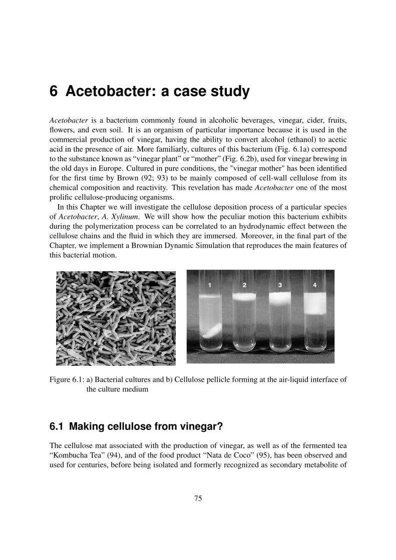
6 Acetobacter: a case study
Acetobacter is a bacterium commonly found in alcoholic beverages, vinegar, cider, fruits,flowers, and even soil. It is an organism of particular importance because it is used in thecommercial production of vinegar, having the ability to convert alcohol (ethanol) to aceticacid in the presence of air. More familiarly, cultures of this bacterium (Fig. 6.1a) correspondto the substance known as “vinegar plant” or “mother” (Fig. 6.2b), used for vinegar brewing inthe old days in Europe. Cultured in pure conditions, the "vinegar mother" has been identifiedfor the first time by Brown (92; 93) to be mainly composed of cell-wall cellulose from itschemical composition and reactivity. This revelation has made Acetobacter one of the mostprolific cellulose-producing organisms.
In this Chapter we will investigate the cellulose deposition process of a particular speciesof Acetobacter, A. Xylinum. We will show how the peculiar motion this bacterium exhibitsduring the polymerization process can be correlated to an hydrodynamic effect between thecellulose chains and the fluid in which they are immersed. Moreover, in the final part of theChapter, we implement a Brownian Dynamic Simulation that reproduces the main features ofthis bacterial motion.
Figure 6.1: a) Bacterial cultures and b) Cellulose pellicle forming at the air-liquid interface ofthe culture medium
6.1 Making cellulose from vinegar?
The cellulose mat associated with the production of vinegar, as well as of the fermented tea“Kombucha Tea” (94), and of the food product “Nata de Coco” (95), has been observed andused for centuries, before being isolated and formerly recognized as secondary metabolite of
75

6 Acetobacter: a case study
the bacterium Acetobacter. Described by Louis Pasteur as “a sort of moist skin, swollen,gelatinous and slippery” substance, this cellulose product has started drawing a scientificinterest only when microscopic observations disclosed bacteria distributed throughout the ma-trix.
Although the solid portion in the gel-like substance is less than one percent by weight, itis almost pure cellulose free of lignin, pectin and hemicellulose as well as other biogenicproducts, which are associated with plant-derived cellulose. This pure cellulose mat can becleaned and dried, and the product used for many applications. One of the unique featuresof the bacterial cellulose membrane is that it is very strong in the dried state, and it can holdhundreds of times its own weight in water. This great absorptivity and mechanical strength,together with the high crystallinity, constitute three of the main features of microbial cellulose.
Figure 6.2: a) Matrix of interwoven ribbons and b) Vinegar mother
The reason why Acetobacter generate cellulose has long been a puzzle for biologists. Onehypothesis is that these aerobic bacteria produce a pellicle to maintain their position close tothe oxygen-rich surface of the culture solution (96; 97). Another theory assumes that the bac-teria generate cellulose to guard themselves from ultraviolet radiation (98). Another opinionis that they use it to construct a “cage” in which they confine themselves to protect themselvesfrom enemies, whereas nutrients can be still supplied by diffusion (99).
6.2 Acetobacter Xylinum
Acetobacter Xylinum is a particular species of Acetobacter. This rod-shaped, motile, non-photosynthetic organism, can be simply grown in a shallow tray with a culture medium suchas coconut juice, sugarcane juice, vinegar, and fermented beverage (100; 101). Starting fromthese materials, it can procure glucose, sugar and other organic substrates and convert theminto pure cellulose. A. Xylinum is nature’s most prolific cellulose-producing bacterium: atypical single cell can convert up to 108 glucose molecules per hour into cellulose. Since abouta million cells can be packed into a large liquid droplet, the amount of cellulose produced bya culture of these bacteria during few hours can be substantial.
76
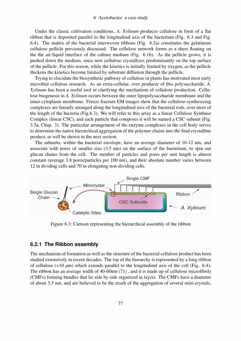
6 Acetobacter: a case study
Under the classic cultivation conditions, A. Xylinum produces cellulose in form of a flatribbon that is deposited parallel to the longitudinal axis of the bacterium (Fig. 6.3 and Fig.6.4). The matrix of the bacterial interwoven ribbons (Fig. 6.2a) constitutes the gelatinouscellulose pellicle previously discussed. The cellulose network forms as a sheet floating onthe the air-liquid interface of the culture medium (Fig. 6.1b). As the pellicle grows, it ispushed down the medium, since new cellulose crystallizes predominantly on the top surfaceof the pellicle. For this reason, while the kinetics is initially limited by oxygen, as the pelliclethickens the kinetics become limited by substrate diffusion through the pellicle.
Trying to elucidate the biosynthetic pathway of cellulose in plants has motivated most earlymicrobial cellulose research. As an extra-cellular, over producer of this polysaccharide, A.Xylinum has been a useful tool in clarifying the mechanism of cellulose production. Cellu-lose biogenesis in A. Xylinum occurs between the outer lipopolysaccharide membrane and theinner cytoplasm membrane. Freeze fracture EM images show that the cellulose-synthesizingcomplexes are linearly arranged along the longitudinal axis of the bacterial rods, over most ofthe length of the bacteria (Fig.6.3). We will refer to this array as a linear Cellulose SynthaseComplex (linear CSC), and each particle that composes it will be named a CSC subunit (Fig.3.3a, Chap. 3). The particular arrangement of the enzyme complexes in the cell body servesto determine the native hierarchical aggregation of the polymer chains into the final crystallineproduct, as will be shown in the next section.
The subunits, within the bacterial envelope, have an average diameter of 10-12 nm, andassociate with pores of smaller size (3.5 nm) on the surface of the bacterium, to spin outglucan chains from the cell. The number of particles and pores per unit length is almostconstant (average 3.8 pores/particles per 100 nm), and their absolute number varies between12 in dividing cells and 70 in elongating non-dividing cells.
Figure 6.3: Cartoon representing the hierarchical assembly of the ribbon
6.2.1 The Ribbon assembly
The mechanism of formation as well as the structure of the bacterial cellulose product has beenstudied extensively in recent decades. The top of the hierarchy is represented by a long ribbonof cellulose (>10 µm) which extends parallel to the longitudinal axis of the cell (Fig. 6.4).The ribbon has an average width of 40-60nm (71) , and it is made up of cellulose microfibrils(CMFs) forming bundles that lie side by side organized in layers. The CMFs have a diameterof about 3.5 nm, and are believed to be the result of the aggregation of several mini-crystals,
77
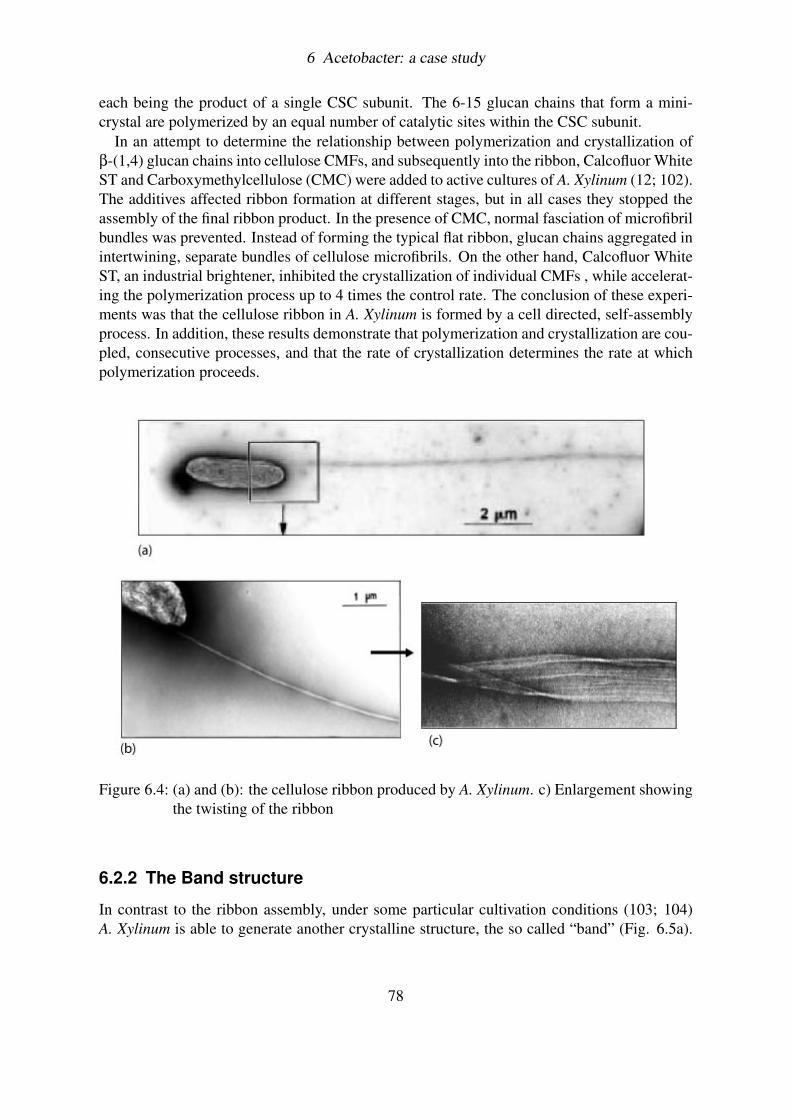
6 Acetobacter: a case study
each being the product of a single CSC subunit. The 6-15 glucan chains that form a mini-crystal are polymerized by an equal number of catalytic sites within the CSC subunit.
In an attempt to determine the relationship between polymerization and crystallization ofβ-(1,4) glucan chains into cellulose CMFs, and subsequently into the ribbon, Calcofluor WhiteST and Carboxymethylcellulose (CMC) were added to active cultures of A. Xylinum (12; 102).The additives affected ribbon formation at different stages, but in all cases they stopped theassembly of the final ribbon product. In the presence of CMC, normal fasciation of microfibrilbundles was prevented. Instead of forming the typical flat ribbon, glucan chains aggregated inintertwining, separate bundles of cellulose microfibrils. On the other hand, Calcofluor WhiteST, an industrial brightener, inhibited the crystallization of individual CMFs , while accelerat-ing the polymerization process up to 4 times the control rate. The conclusion of these experi-ments was that the cellulose ribbon in A. Xylinum is formed by a cell directed, self-assemblyprocess. In addition, these results demonstrate that polymerization and crystallization are cou-pled, consecutive processes, and that the rate of crystallization determines the rate at whichpolymerization proceeds.
Figure 6.4: (a) and (b): the cellulose ribbon produced by A. Xylinum. c) Enlargement showingthe twisting of the ribbon
6.2.2 The Band structure
In contrast to the ribbon assembly, under some particular cultivation conditions (103; 104)A. Xylinum is able to generate another crystalline structure, the so called “band” (Fig. 6.5a).
78
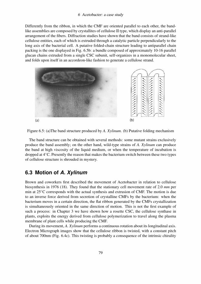
6 Acetobacter: a case study
Differently from the ribbon, in which the CMF are oriented parallel to each other, the band-like assemblies are composed by crystallites of cellulose II type, which display an anti-parallelarrangement of the fibers. Diffraction studies have shown that the band consists of strand-likecellulose entities, each of which is extruded through a catalytic particle perpendicularly to thelong axis of the bacterial cell. A putative folded-chain structure leading to antiparallel chainpacking is the one displayed in Fig. 6.5b: a bundle composed of approximately 10-16 parallelglucan chains extruded from a single CSC subunit, self-organizes in a monomolecular sheet,and folds upon itself in an accordeon-like fashion to generate a cellulose strand.
Figure 6.5: (a)The band structure produced by A. Xylinum. (b) Putative folding mechanism
The band structure can be obtained with several methods: some mutant strains exclusivelyproduce the band assembly; on the other hand, wild-type strains of A. Xylinum can producethe band at high viscosity of the liquid medium, or when the temperature of incubation isdropped at 4C. Presently the reason that makes the bacterium switch between these two typesof cellulose structure is shrouded in mystery.
6.3 Motion of A. Xylinum
Brown and coworkers first described the movement of Acetobacter in relation to cellulosebiosynthesis in 1976 (18). They found that the stationary cell movement rate of 2.0 mm permin at 25C corresponds with the actual synthesis and extrusion of CMF. The motion is dueto an inverse force derived from secretion of crystalline CMFs by the bacterium: when thebacterium moves in a certain direction, the flat ribbon generated by the CMFs crystallizationis simultaneously oriented in the same direction of motion. This is not the first example ofsuch a process: in Chapter 3 we have shown how a rosette CSC, the cellulose synthase inplants, exploits the energy derived from cellulose polymerization to travel along the plasmamembrane of plant cells while producing the CMF.
During its movement, A. Xylinum performs a continuous rotation about its longitudinal axis.Electron Micrograph images show that the cellulose ribbon is twisted, with a constant pitchof about 700nm (Fig. 6.4c). This twisting is probably a consequence of the intrinsic chirality
79
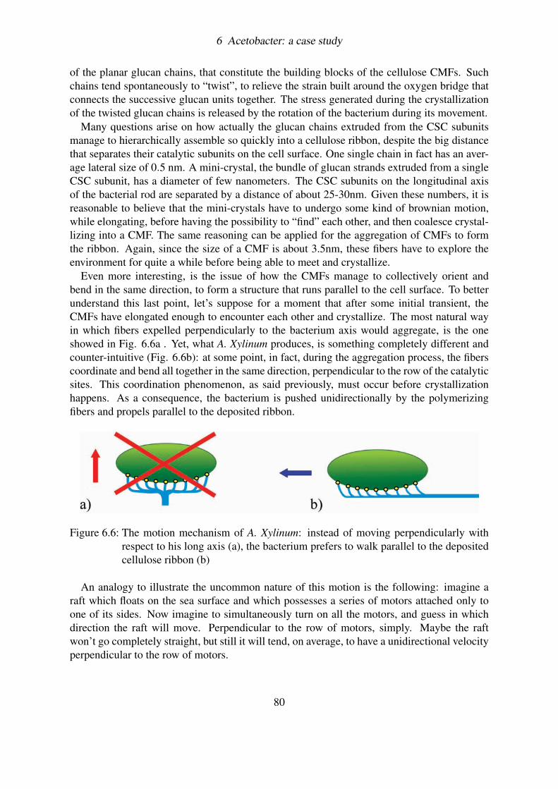
6 Acetobacter: a case study
of the planar glucan chains, that constitute the building blocks of the cellulose CMFs. Suchchains tend spontaneously to “twist”, to relieve the strain built around the oxygen bridge thatconnects the successive glucan units together. The stress generated during the crystallizationof the twisted glucan chains is released by the rotation of the bacterium during its movement.
Many questions arise on how actually the glucan chains extruded from the CSC subunitsmanage to hierarchically assemble so quickly into a cellulose ribbon, despite the big distancethat separates their catalytic subunits on the cell surface. One single chain in fact has an aver-age lateral size of 0.5 nm. A mini-crystal, the bundle of glucan strands extruded from a singleCSC subunit, has a diameter of few nanometers. The CSC subunits on the longitudinal axisof the bacterial rod are separated by a distance of about 25-30nm. Given these numbers, it isreasonable to believe that the mini-crystals have to undergo some kind of brownian motion,while elongating, before having the possibility to “find” each other, and then coalesce crystal-lizing into a CMF. The same reasoning can be applied for the aggregation of CMFs to formthe ribbon. Again, since the size of a CMF is about 3.5nm, these fibers have to explore theenvironment for quite a while before being able to meet and crystallize.
Even more interesting, is the issue of how the CMFs manage to collectively orient andbend in the same direction, to form a structure that runs parallel to the cell surface. To betterunderstand this last point, let’s suppose for a moment that after some initial transient, theCMFs have elongated enough to encounter each other and crystallize. The most natural wayin which fibers expelled perpendicularly to the bacterium axis would aggregate, is the oneshowed in Fig. 6.6a . Yet, what A. Xylinum produces, is something completely different andcounter-intuitive (Fig. 6.6b): at some point, in fact, during the aggregation process, the fiberscoordinate and bend all together in the same direction, perpendicular to the row of the catalyticsites. This coordination phenomenon, as said previously, must occur before crystallizationhappens. As a consequence, the bacterium is pushed unidirectionally by the polymerizingfibers and propels parallel to the deposited ribbon.
Figure 6.6: The motion mechanism of A. Xylinum: instead of moving perpendicularly withrespect to his long axis (a), the bacterium prefers to walk parallel to the depositedcellulose ribbon (b)
An analogy to illustrate the uncommon nature of this motion is the following: imagine araft which floats on the sea surface and which possesses a series of motors attached only toone of its sides. Now imagine to simultaneously turn on all the motors, and guess in whichdirection the raft will move. Perpendicular to the row of motors, simply. Maybe the raftwon’t go completely straight, but still it will tend, on average, to have a unidirectional velocityperpendicular to the row of motors.
80
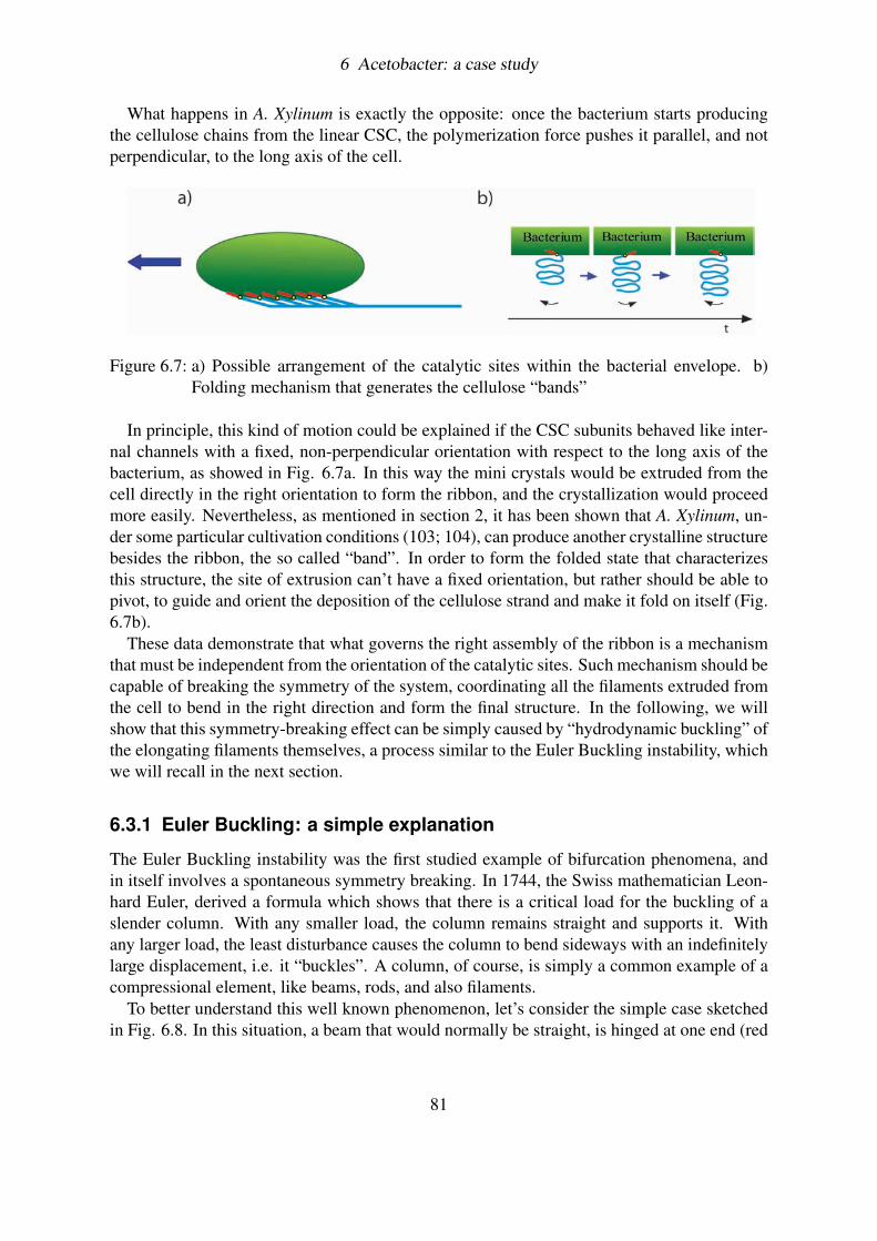
6 Acetobacter: a case study
What happens in A. Xylinum is exactly the opposite: once the bacterium starts producingthe cellulose chains from the linear CSC, the polymerization force pushes it parallel, and notperpendicular, to the long axis of the cell.
Figure 6.7: a) Possible arrangement of the catalytic sites within the bacterial envelope. b)Folding mechanism that generates the cellulose “bands”
In principle, this kind of motion could be explained if the CSC subunits behaved like inter-nal channels with a fixed, non-perpendicular orientation with respect to the long axis of thebacterium, as showed in Fig. 6.7a. In this way the mini crystals would be extruded from thecell directly in the right orientation to form the ribbon, and the crystallization would proceedmore easily. Nevertheless, as mentioned in section 2, it has been shown that A. Xylinum, un-der some particular cultivation conditions (103; 104), can produce another crystalline structurebesides the ribbon, the so called “band”. In order to form the folded state that characterizesthis structure, the site of extrusion can’t have a fixed orientation, but rather should be able topivot, to guide and orient the deposition of the cellulose strand and make it fold on itself (Fig.6.7b).
These data demonstrate that what governs the right assembly of the ribbon is a mechanismthat must be independent from the orientation of the catalytic sites. Such mechanism should becapable of breaking the symmetry of the system, coordinating all the filaments extruded fromthe cell to bend in the right direction and form the final structure. In the following, we willshow that this symmetry-breaking effect can be simply caused by “hydrodynamic buckling” ofthe elongating filaments themselves, a process similar to the Euler Buckling instability, whichwe will recall in the next section.
6.3.1 Euler Buckling: a simple explanation
The Euler Buckling instability was the first studied example of bifurcation phenomena, andin itself involves a spontaneous symmetry breaking. In 1744, the Swiss mathematician Leon-hard Euler, derived a formula which shows that there is a critical load for the buckling of aslender column. With any smaller load, the column remains straight and supports it. Withany larger load, the least disturbance causes the column to bend sideways with an indefinitelylarge displacement, i.e. it “buckles”. A column, of course, is simply a common example of acompressional element, like beams, rods, and also filaments.
To better understand this well known phenomenon, let’s consider the simple case sketchedin Fig. 6.8. In this situation, a beam that would normally be straight, is hinged at one end (red
81
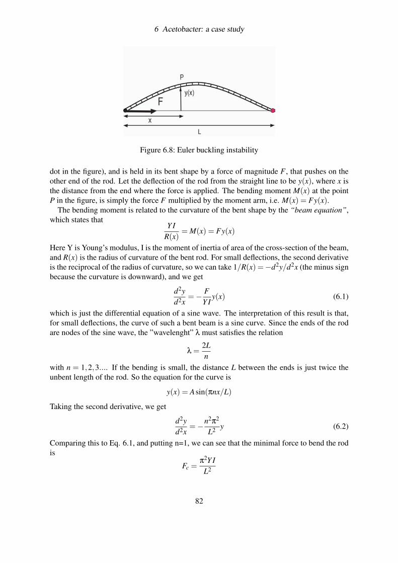
6 Acetobacter: a case study
Figure 6.8: Euler buckling instability
dot in the figure), and is held in its bent shape by a force of magnitude F , that pushes on theother end of the rod. Let the deflection of the rod from the straight line to be y(x), where x isthe distance from the end where the force is applied. The bending moment M(x) at the pointP in the figure, is simply the force F multiplied by the moment arm, i.e. M(x) = Fy(x).
The bending moment is related to the curvature of the bent shape by the “beam equation”,which states that
Y IR(x)
= M(x) = Fy(x)
Here Y is Young’s modulus, I is the moment of inertia of area of the cross-section of the beam,and R(x) is the radius of curvature of the bent rod. For small deflections, the second derivativeis the reciprocal of the radius of curvature, so we can take 1/R(x) =−d2y/d2x (the minus signbecause the curvature is downward), and we get
d2yd2x
=− FY I
y(x) (6.1)
which is just the differential equation of a sine wave. The interpretation of this result is that,for small deflections, the curve of such a bent beam is a sine curve. Since the ends of the rodare nodes of the sine wave, the ”wavelenght” λ must satisfies the relation
λ =2Ln
with n = 1,2,3.... If the bending is small, the distance L between the ends is just twice theunbent length of the rod. So the equation for the curve is
y(x) = Asin(πnx/L)
Taking the second derivative, we get
d2yd2x
=−n2π2
L2 y (6.2)
Comparing this to Eq. 6.1, and putting n=1, we can see that the minimal force to bend the rodis
Fc =π2Y I
L2
82
6 Acetobacter: a case study
Note that for small bending the force is independent of the bending displacement y(x).We have, then, the following result physically: Fc, often called “Euler force”, is the force
above which the beam is unstable and suddenly bends a large amount, buckling. It is foundfrom practice that this theory gives good results for columns and filaments that are more than30 times longer than wide. As one can clearly see, Fc is proportional to 1/L2, so the sup-porting capacity of a column decreases rapidly with an increase in length. Moreover, lookingat the equation for the bending moment M(x), it is possible to see that M(x) increases withthe displacement y(x), meaning that any buckling merely encourages further buckling. Thisexplains why such failure is catastrophic.
6.4 Hydrodynamic Buckling
Of course, everything discussed above is valid only for small bending of the beam. Whenthe displacement gets large the approximation 1/R(x) = −d2y/d2x is no more valid. To findthe force necessary to bend the rod for a large deformation of the beam, we should proceedin a more detailed and correct way, taking into account the complete energy functional of therod. This more general description is also useful because it allows us to derive the bucklingphenomenon for different systems, for example for a filament immersed in a viscous liquidlike in the case of Acetobacter cellulose chains.
Our aim in this section is to derive the mathematical conditions that determine the bucklingtransition for a semiflexible filament which is moving in a fluid with a velocity v. Our idea isthat the elongation of the cellulose chain from the bacterial catalytic site is able to generate,when the chain approaches a critical length Lc, an instability similar to the one described byEuler for the bending of columns. However, in this case, differently from Euler buckling, thereis no constant force pushing the end of the filament. Rather, what determines the bucklinginstability, is the viscous drag that the fluid exerts on the elongating filament itself.
To understand this concept more easily, remember that to make a rod of length L move in afluid of viscosity η with a tangential velocity v‖, it is necessary to apply a pushing force equalto:
F = v‖ξ‖L
where, according to the slender-body theory (105), the tangential friction coefficient, ξ‖ =2πη/[ln(2L)− 0.5]. As you can see from this formula, the greater the length of the rod L,bigger the force you have to apply to maintain the velocity v‖. Imagine now a filament that iselongating in a viscous medium with a constant velocity, like, for example, a cellulose chainbeing polymerized by A. Xylinum. At the beginning the filament is very short, and the resistingfriction force it experiences is very small. However, when the length reaches a certain criticalvalue Lc, the viscous force is so big to hydrodynamically “buckle” the filament, in the sameway as was discussed previously for the Euler instability.
In the following paragraphs we mathematically derive this critical length, and we demon-strate that the hydrodynamic buckling can serve as an explanation for the breaking of sym-metry that occurs during the polymerization process of A. Xylinum, and also as a basic phe-nomenon to understand the longitudinal motion of this bacterium .
83
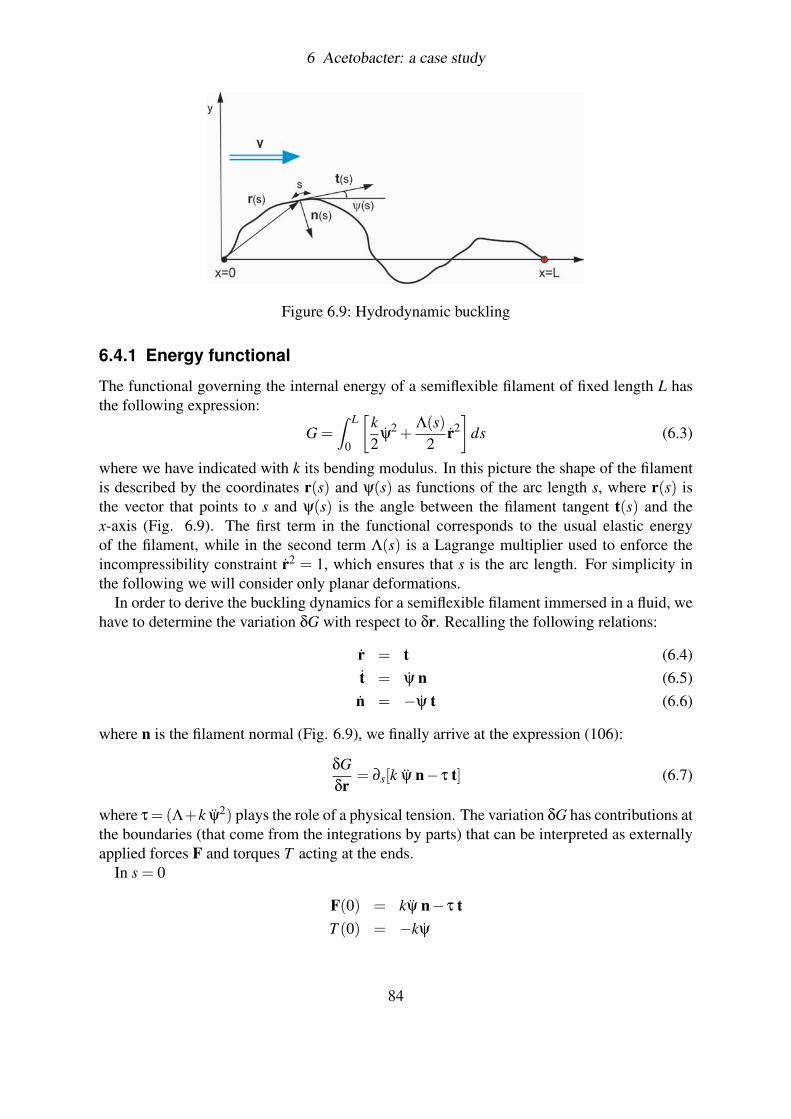
6 Acetobacter: a case study
Figure 6.9: Hydrodynamic buckling
6.4.1 Energy functional
The functional governing the internal energy of a semiflexible filament of fixed length L hasthe following expression:
G =Z L
0
[k2
ψ2 +
Λ(s)2
r2]
ds (6.3)
where we have indicated with k its bending modulus. In this picture the shape of the filamentis described by the coordinates r(s) and ψ(s) as functions of the arc length s, where r(s) isthe vector that points to s and ψ(s) is the angle between the filament tangent t(s) and thex-axis (Fig. 6.9). The first term in the functional corresponds to the usual elastic energyof the filament, while in the second term Λ(s) is a Lagrange multiplier used to enforce theincompressibility constraint r2 = 1, which ensures that s is the arc length. For simplicity inthe following we will consider only planar deformations.
In order to derive the buckling dynamics for a semiflexible filament immersed in a fluid, wehave to determine the variation δG with respect to δr. Recalling the following relations:
r = t (6.4)t = ψ n (6.5)n = −ψ t (6.6)
where n is the filament normal (Fig. 6.9), we finally arrive at the expression (106):
δGδr
= ∂s[k ψ n− τ t] (6.7)
where τ = (Λ+k ψ2) plays the role of a physical tension. The variation δG has contributions atthe boundaries (that come from the integrations by parts) that can be interpreted as externallyapplied forces F and torques T acting at the ends.
In s = 0
F(0) = kψ n− τ tT (0) = −kψ
84
6 Acetobacter: a case study
while in s = L
F(L) = −kψ n+ τ tT (L) = kψ.
These value will be fixed by the initial conditions of the problem.
6.4.2 Dynamic equations
Now that we have the expression for the functional derivative δGδr , we can focus on the dy-
namics of an elastic filament immersed in a low Reynolds number fluid. In fluid mechanicsthe Reynolds number Re=ρvl/η, is the ratio of inertial forces (vρ) to viscous forces (η/l) andis used to determine whether a flow is laminar or turbulent. Here v is the fluid velocity, ρ isthe fluid density, η the fluid viscosity and l is a characteristic length of the system. Laminarflow occurs at low Reynolds numbers (Re < 2100), where viscous forces are dominant, andis characterized by smooth, constant fluid motion. Turbulent flow, on the other hand, occursat high Reynolds numbers (Re> 4000) and is dominated by inertial forces, producing vertexesand other flow fluctuations.
If we are interested in studying the dynamics of biological filaments, we are concernednearly always with the low Reynolds number regime. In fact, because of their size and typicalvelocities, inertia is essentially irrelevant for these kind of systems. It is thus possible to use asimplified description for the filament dynamics, namely through an over-damped (negligiblemass) equation of motion, that can be written as:
(∂tr−v) =−
(1
ξ⊥nn+
1ξ‖
tt
)· δG
δr. (6.8)
Here, ∂tr is the local velocity of the polymer, and v is any background velocity that may bepresent in the problem. Following slender-body theory, the effect of the surrounding fluid istaken as a drag force that is proportional and opposite to the local velocity. This is anisotropicdue to the elongated shape of the filament. We therefore require two different local frictioncoefficients, ξ‖ and ξ⊥, for tangential and normal motion, respectively: ξ‖ is associated withthe projector tt along the tangent vector t, while ξ⊥ corresponds to the projector nn and actsalong the normal vector n. Each of these coefficients (per unit length) is intended to be con-stant, i.e. in the following we will neglect their weak logarithmic dependence on the length Lof the filament.
In order to study the hydrodynamic buckling for a semiflexible filament of fixed length L,we start by focusing on an initially straight polymer that is anchored with one end in x = L.We then may consider either forcing the filament by longitudinally moving the anchor witha negative velocity v = −v ex), or moving the fluid relative to the polymer with a positivevelocity, v = v ex. In the following, for sake of simplicity, we are going to solve the Eq. 6.8with the boundary conditions referred to the latter case. However, the equivalence of the twosystems will be provided by the comparison of the theoretical results with the simulations thatwill be presented later on.
85
6 Acetobacter: a case study
Substituting the expression for δG/δr found in the previous section we have:
∂tr =n
ξ⊥(−k
...ψ + ψτ)+
tξ‖
(kψψ+ τ)+v. (6.9)
The tension τ is determined by the constraint of incompressibility ∂tt2 = 2t · ∂tt = 0. Thiscondition leads to a differential equation for the tension profile (106):
τ−ξ‖ξ⊥
ψ2τ =−k∂s(ψψ)− k
ξ‖ξ⊥
ψ...ψ + ψv⊥− v‖. (6.10)
where v‖ and v⊥ are the component of the fluid velocity along the tangential and normaldirection, respectively.
6.4.3 Linearized equation
Let’s consider the case of a filament of length L initially lying along the horizontal axis andhinged in x = L. Let’s assume that the velocity of the fluid runs along the x-axis too, i.e.v = v ex, as depicted in Fig. 6.9. At the linear order, for small deviation from a horizontal line,s' x, t' ex, n'−ey, ψ = y, and we can rewrite the Eqs. 6.9 and 6.10 as:
ξ⊥∂ty = (−k....y + τ y)
ξ‖∂tx = (τ+ v ξ‖)
andτ = 0 (6.11)
Since the filament is hinged in x = L we have ∂ty(L) = ∂tx(L) = 0, from which it follows thatτ(L) = −v ξ‖ . This result, together with eq.(6.11), leads to τ(x) = −v ξ‖. Now we look atthe boundary conditions at the free end. Since there are no external forces acting in x = 0, wefind from eq. (6.8) that (F(0) · ex) =−τ(0) = 0, that leads us to the expression for the tensionbehaviour along the filament, τ(x) = −v ξ‖ x. Substituting this result in eq. (6.11) we finallyobtain:
ξ⊥∂ty = (−k....y − v ξ‖ x y) (6.12)
This is the simplest linearized expression we will work on. As we intuitively expect,y(x, t) ≡ 0 ∀x, t is clearly a trivial solution of this equation, corresponding to the completelystiff horizontal configuration of the filament. This solution is however stable only for smallvalues of v. In fact, as in normal buckling phenomena, when the critical force acting on thefree end of the filament exceeds a critical values Fc, the filament buckles. In our case, as al-ready said, the force is due to the viscous drag, and consequently it increases as the length L ofthe filament or the fluid velocity v increase. For a filament of fixed length L, at a certain criticalvelocity vc the viscous force becomes so strong to buckle the rod. This case corresponds to anon-trivial solution for y(x, t).
86
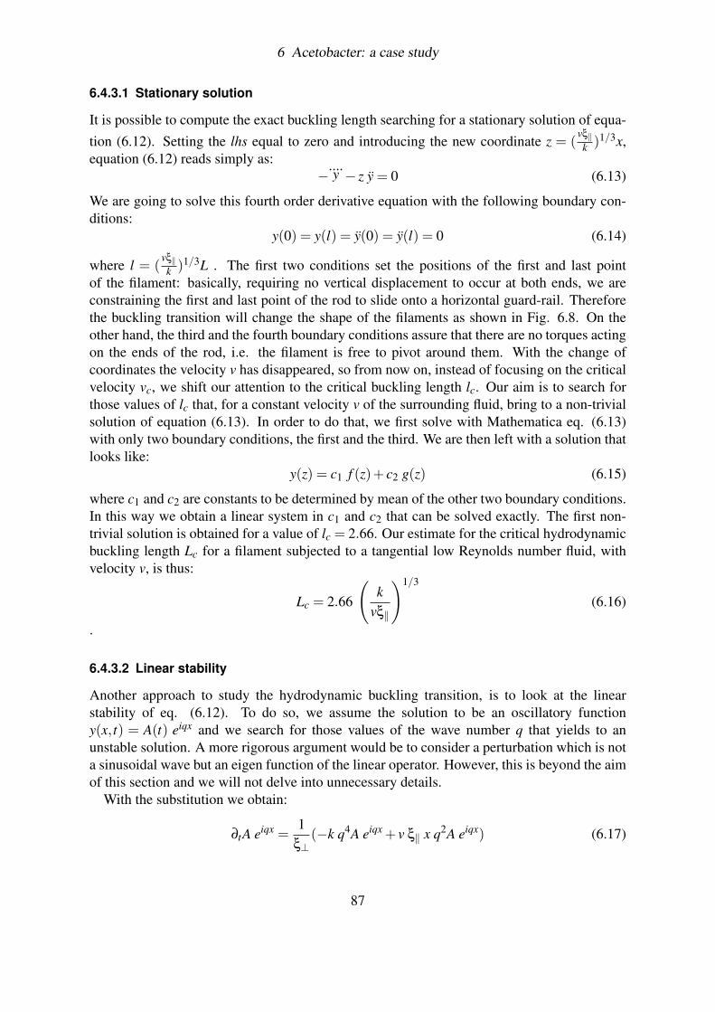
6 Acetobacter: a case study
6.4.3.1 Stationary solution
It is possible to compute the exact buckling length searching for a stationary solution of equa-tion (6.12). Setting the lhs equal to zero and introducing the new coordinate z = (
vξ‖k )1/3x,
equation (6.12) reads simply as:−
....y − z y = 0 (6.13)
We are going to solve this fourth order derivative equation with the following boundary con-ditions:
y(0) = y(l) = y(0) = y(l) = 0 (6.14)
where l = (vξ‖k )1/3L . The first two conditions set the positions of the first and last point
of the filament: basically, requiring no vertical displacement to occur at both ends, we areconstraining the first and last point of the rod to slide onto a horizontal guard-rail. Thereforethe buckling transition will change the shape of the filaments as shown in Fig. 6.8. On theother hand, the third and the fourth boundary conditions assure that there are no torques actingon the ends of the rod, i.e. the filament is free to pivot around them. With the change ofcoordinates the velocity v has disappeared, so from now on, instead of focusing on the criticalvelocity vc, we shift our attention to the critical buckling length lc. Our aim is to search forthose values of lc that, for a constant velocity v of the surrounding fluid, bring to a non-trivialsolution of equation (6.13). In order to do that, we first solve with Mathematica eq. (6.13)with only two boundary conditions, the first and the third. We are then left with a solution thatlooks like:
y(z) = c1 f (z)+ c2 g(z) (6.15)
where c1 and c2 are constants to be determined by mean of the other two boundary conditions.In this way we obtain a linear system in c1 and c2 that can be solved exactly. The first non-trivial solution is obtained for a value of lc = 2.66. Our estimate for the critical hydrodynamicbuckling length Lc for a filament subjected to a tangential low Reynolds number fluid, withvelocity v, is thus:
Lc = 2.66
(k
vξ‖
)1/3
(6.16)
.
6.4.3.2 Linear stability
Another approach to study the hydrodynamic buckling transition, is to look at the linearstability of eq. (6.12). To do so, we assume the solution to be an oscillatory functiony(x, t) = A(t) eiqx and we search for those values of the wave number q that yields to anunstable solution. A more rigorous argument would be to consider a perturbation which is nota sinusoidal wave but an eigen function of the linear operator. However, this is beyond the aimof this section and we will not delve into unnecessary details.
With the substitution we obtain:
∂tA eiqx =1
ξ⊥(−k q4A eiqx + v ξ‖ x q2A eiqx) (6.17)
87

6 Acetobacter: a case study
Setting ω(q) =−kq4 + vξ‖xq2 and cancelling the exponential we are left with the expression:
∂tA = ω(q) A (6.18)
which has a solutionA(t) = A(0) eω(q)t (6.19)
This solution in stable and converges to zero only for negative values of ω(q) Therefore, we
can say that the filament buckles whenever ω(q) > 0, i.e. q2 <v ξ‖ x
k . For a filament of lengthL with both ends fixed in y = 0, the allowed wave numbers are only the ones that satisfy therelation q = nπ/L, with n being an integer. This means that the filament buckles whenever
L2 >π2k
v ξ‖ x(6.20)
where since we are interested in the first non-trivial solution we have put n = 1. The expression(6.20) is a bit nasty since it depends on the unknown quantity x. To get rid of it we repeatthe same procedure described at the beginning of this section, for the symmetric case of ourproblem, the one in which we have the filament hinged in x = 0 and subjected to a fluidvelocity v =−v ex. For symmetry considerations we have to find the same buckling length Lc.
0 10 20 30 40 50 60L
0
0.2
0.4
0.6
0.8
1
d/L
k=10k=50k=150k=300k=500k=700k=1000
Figure 6.10: Buckling transitions for different values of the bending parameter k
Doing all the calculations for the symmetric case we finally arrive at a similar expression,except for the fact that instead of x we have now (L−x). This implies that in this case ω(q) > 0whenever L2 > π2k
v ξ‖ (L−x) .
88
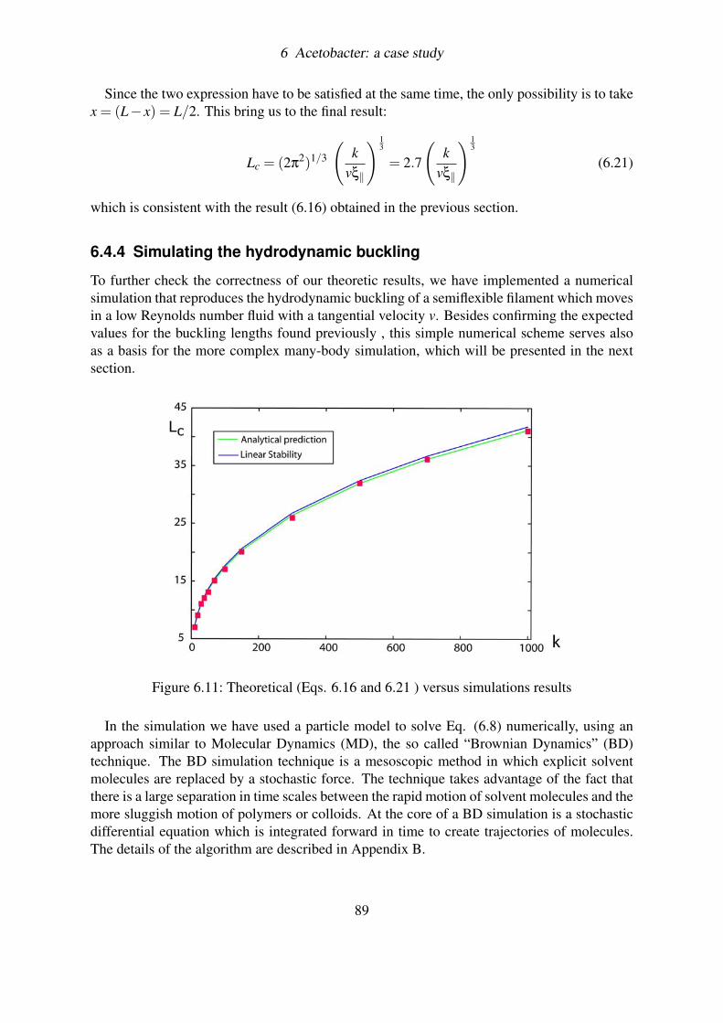
6 Acetobacter: a case study
Since the two expression have to be satisfied at the same time, the only possibility is to takex = (L− x) = L/2. This bring us to the final result:
Lc = (2π2)1/3
(k
vξ‖
) 13
= 2.7
(k
vξ‖
) 13
(6.21)
which is consistent with the result (6.16) obtained in the previous section.
6.4.4 Simulating the hydrodynamic buckling
To further check the correctness of our theoretic results, we have implemented a numericalsimulation that reproduces the hydrodynamic buckling of a semiflexible filament which movesin a low Reynolds number fluid with a tangential velocity v. Besides confirming the expectedvalues for the buckling lengths found previously , this simple numerical scheme serves alsoas a basis for the more complex many-body simulation, which will be presented in the nextsection.
Figure 6.11: Theoretical (Eqs. 6.16 and 6.21 ) versus simulations results
In the simulation we have used a particle model to solve Eq. (6.8) numerically, using anapproach similar to Molecular Dynamics (MD), the so called “Brownian Dynamics” (BD)technique. The BD simulation technique is a mesoscopic method in which explicit solventmolecules are replaced by a stochastic force. The technique takes advantage of the fact thatthere is a large separation in time scales between the rapid motion of solvent molecules and themore sluggish motion of polymers or colloids. At the core of a BD simulation is a stochasticdifferential equation which is integrated forward in time to create trajectories of molecules.The details of the algorithm are described in Appendix B.
89

6 Acetobacter: a case study
In our model, time is discretized and the filament is described as a set of n particles of diam-eter σ rigidly connected by n−1 links. The stochastic force, that depends on the temperatureT , is the source of fluctuations that makes the buckling transition possible. In fact, in absenceof any noise (T = 0), a straight filament pushed along its longitudinal direction won’t buckle atall in a numerical simulation, because there would be no transversal components of the forceto bend it. The role of the stochastic force is thus to introduce the small fluctuations necessaryto break the symmetry. However, in order to compare the numerical results to the theory, wehave performed the simulations with T → 0. This also makes an accurate evaluation of thebuckling lengths easier, because the data are less noisy and the transitions more pronounced.
We consider a filament of fixed length L = nσ, initially lying along the horizontal direction,that is longitudinally moving with a constant velocity v in a low Reynolds number fluid. Fol-lowing the boundary conditions given by Eq. (6.14), both ends of the filament are constrainedto slide on a horizontal guide rail and they can’t experience any vertical displacement. Inaddition, the ends of the filaments are not clamped, i.e. there are no torques acting on them.
We define our order parameter ψ = d/L, as the ratio of the distance 0 < d < L between theends, and the contour length L of the filament. At the beginning of the simulation the rod isstraight, i.e. ψ = 1. Then the filament is pushed in the fluid with a velocity v for a time t untilit reaches a stationary configuration. If the filament is very short, or very stiff, then the orderparameter of the stationary configuration remains always around the value ψ' 1. For greaterfilament lengths L, or a smaller bending constant k, the rod buckles, and the order parameterψ → 0. In Fig. 6.10, each curve shows the result of a single run of simulations, in whichwe have measured the value of the order parameter ψ as a function of the filament length L,with the stiffness k, the velocity v and the viscosity η of the fluid kept constant. The criticalbuckling length Lc is identified as the last value of L for which ψ = 1. Repeating the samerun of simulations for different values of the bending parameter k, we obtain all the curvesdisplayed in Fig. 6.10.
The buckling transition is very pronounced: the value of the order parameter drops verysharply form 1 to 0. If we plot the critical lengths versus the bending parameter k, we cancompare the simulation with the theoretically predicted behaviour of the previous sections(Fig. 6.11). As one can clearly see, the agreement is excellent.
6.4.5 Discussion on results
The persistence length Lp of a single cellulose chain in aqueous solution has been estimatedby MD simulations (107), which provide an upper limit of Lp = 14.5±1nm. The persistencelength is related to the bending modulus k by the relation Lp = k/KBT , and at room tem-perature this corresponds to a value of k = 5.6 10−29Nm2. The parallel drag coefficient of afilament, neglecting the weak logarithmic dependence on its length, is ξ‖ ' 2πη, where η isthe viscosity of the medium in which the filament is dipped. In our case we have η = 1cP(viscosity of water) so that ξ‖ ' 6.2 10−3cP. We put the velocity at which the filament isdipped into the medium equal to the polymerization velocity of cellulose, v = 12 10−8m/s.Substituting these values in the Eq. 6.16, we find that the buckling length at which a poly-merizing cellulose chain is bent is Lc ' 1.1 10−6m. If we repeat the same procedure for the
90
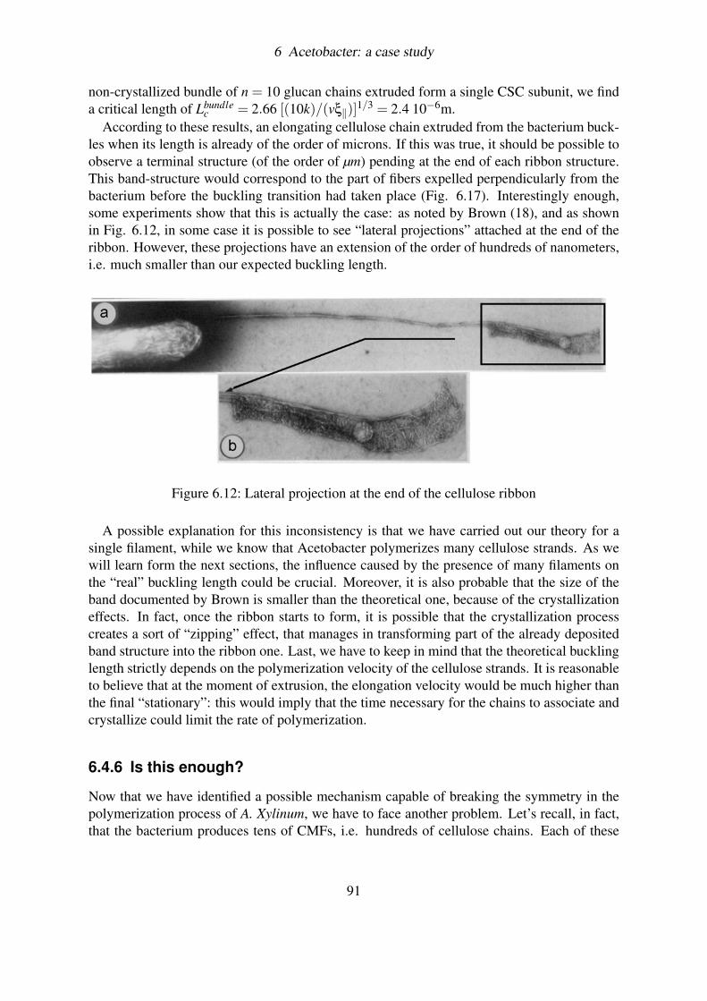
6 Acetobacter: a case study
non-crystallized bundle of n = 10 glucan chains extruded form a single CSC subunit, we finda critical length of Lbundle
c = 2.66 [(10k)/(vξ‖)]1/3 = 2.4 10−6m.According to these results, an elongating cellulose chain extruded from the bacterium buck-
les when its length is already of the order of microns. If this was true, it should be possible toobserve a terminal structure (of the order of µm) pending at the end of each ribbon structure.This band-structure would correspond to the part of fibers expelled perpendicularly from thebacterium before the buckling transition had taken place (Fig. 6.17). Interestingly enough,some experiments show that this is actually the case: as noted by Brown (18), and as shownin Fig. 6.12, in some case it is possible to see “lateral projections” attached at the end of theribbon. However, these projections have an extension of the order of hundreds of nanometers,i.e. much smaller than our expected buckling length.
Figure 6.12: Lateral projection at the end of the cellulose ribbon
A possible explanation for this inconsistency is that we have carried out our theory for asingle filament, while we know that Acetobacter polymerizes many cellulose strands. As wewill learn form the next sections, the influence caused by the presence of many filaments onthe “real” buckling length could be crucial. Moreover, it is also probable that the size of theband documented by Brown is smaller than the theoretical one, because of the crystallizationeffects. In fact, once the ribbon starts to form, it is possible that the crystallization processcreates a sort of “zipping” effect, that manages in transforming part of the already depositedband structure into the ribbon one. Last, we have to keep in mind that the theoretical bucklinglength strictly depends on the polymerization velocity of the cellulose strands. It is reasonableto believe that at the moment of extrusion, the elongation velocity would be much higher thanthe final “stationary”: this would imply that the time necessary for the chains to associate andcrystallize could limit the rate of polymerization.
6.4.6 Is this enough?
Now that we have identified a possible mechanism capable of breaking the symmetry in thepolymerization process of A. Xylinum, we have to face another problem. Let’s recall, in fact,that the bacterium produces tens of CMFs, i.e. hundreds of cellulose chains. Each of these
91
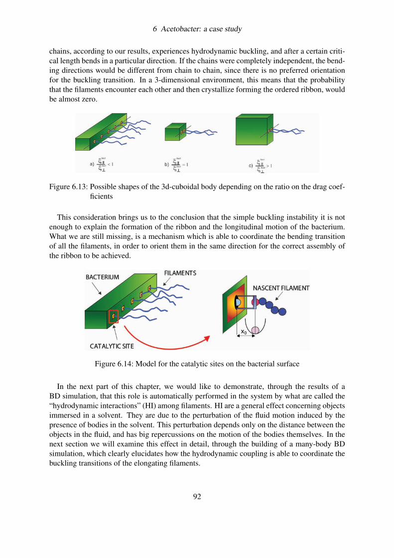
6 Acetobacter: a case study
chains, according to our results, experiences hydrodynamic buckling, and after a certain criti-cal length bends in a particular direction. If the chains were completely independent, the bend-ing directions would be different from chain to chain, since there is no preferred orientationfor the buckling transition. In a 3-dimensional environment, this means that the probabilitythat the filaments encounter each other and then crystallize forming the ordered ribbon, wouldbe almost zero.
Figure 6.13: Possible shapes of the 3d-cuboidal body depending on the ratio on the drag coef-ficients
This consideration brings us to the conclusion that the simple buckling instability it is notenough to explain the formation of the ribbon and the longitudinal motion of the bacterium.What we are still missing, is a mechanism which is able to coordinate the bending transitionof all the filaments, in order to orient them in the same direction for the correct assembly ofthe ribbon to be achieved.
Figure 6.14: Model for the catalytic sites on the bacterial surface
In the next part of this chapter, we would like to demonstrate, through the results of aBD simulation, that this role is automatically performed in the system by what are called the“hydrodynamic interactions” (HI) among filaments. HI are a general effect concerning objectsimmersed in a solvent. They are due to the perturbation of the fluid motion induced by thepresence of bodies in the solvent. This perturbation depends only on the distance between theobjects in the fluid, and has big repercussions on the motion of the bodies themselves. In thenext section we will examine this effect in detail, through the building of a many-body BDsimulation, which clearly elucidates how the hydrodynamic coupling is able to coordinate thebuckling transitions of the elongating filaments.
92
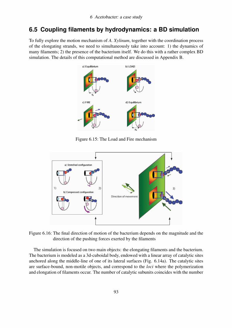
6 Acetobacter: a case study
6.5 Coupling filaments by hydrodynamics: a BD simulation
To fully explore the motion mechanism of A. Xylinum, together with the coordination processof the elongating strands, we need to simultaneously take into account: 1) the dynamics ofmany filaments; 2) the presence of the bacterium itself. We do this with a rather complex BDsimulation. The details of this computational method are discussed in Appendix B.
Figure 6.15: The Load and Fire mechanism
Figure 6.16: The final direction of motion of the bacterium depends on the magnitude and thedirection of the pushing forces exerted by the filaments
The simulation is focused on two main objects: the elongating filaments and the bacterium.The bacterium is modeled as a 3d-cuboidal body, endowed with a linear array of catalytic sitesanchored along the middle-line of one of its lateral surfaces (Fig. 6.14a). The catalytic sitesare surface-bound, non-motile objects, and correspond to the loci where the polymerizationand elongation of filaments occur. The number of catalytic subunits coincides with the number
93
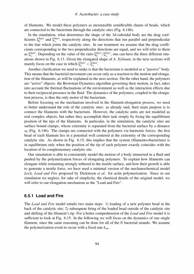
6 Acetobacter: a case study
of filaments. We model these polymers as inextensible semiflexible chains of beads, whichare connected to the bacterium through the catalytic sites (Fig. 6.14b).
In the simulation, what determines the shape of the 3d-cuboidal body are the drag coef-ficients ξbact
‖ and ξbact⊥ , respectively along the directions that run parallel and perpendicular
to the line which joints the catalytic sites. In our treatment we assume that the drag coeffi-cients corresponding to the two perpendicular directions are equal, and we will refer to themas ξbact
⊥ . Depending on the value of the ratio ξbact‖ /ξbact
⊥ , one can have the three different situ-ations shown in Fig. 6.13. Given the elongated shape of A. Xylinum, in the next sections willmainly focus on the case in which ξbact
‖ < ξbact⊥ .
Another clarification we need to make is that the bacterium is modeled as a “passive” body.This means that the bacterial movement can occur only as a reaction to the motion and elonga-tion of the filaments, as will be explained in the next section. On the other hand, the polymersare “active” objects: the Brownian Dynamics algorithm governing their motion, in fact, takesinto account the thermal fluctuations of the environment as well as the interaction effects dueto their reciprocal presence in the fluid. The dynamics of the polymers, coupled to the elonga-tion process, is thus the only motor of the bacterium.
Before focusing on the mechanism involved in the filament-elongation process, we needto better understand the role of the catalytic sites: as already said, their main purpose is toconnect the filaments with the bacterium. However, the catalytic units are not modeled asreal complex objects, but rather they accomplish their task simply by fixing the equilibriumposition of the tips of the filaments. In particular, in the simulation, the catalytic sites aresurface bound clamps, whose extremity is separated from the bacterial surface by a distancex0 (Fig. 6.14b). The clamps are connected with the polymers via harmonic forces: the firstbead of each filament lies in a potential well centered at the extremity of the correspondingcatalytic site. As shown in Fig. 6.15, this implies that the system (filaments+bacterium) isin equilibrium only when the position of the tip of each polymer exactly coincides with thelocation of its complementary catalytic site.
Our simulation is able to consistently model the motion of a body immersed in a fluid andpushed by the polymerization forces of elongating polymers. To explain how filaments canelongate while remaining strongly tethered to the motile surface, and how their growth is ableto generate a motile force, we have used a minimal version of the mechanochemical modelLock, Load and Fire proposed by Dickinson et al. for actin polymerization. Since in oursimulation we neglect, for sake of simplicity, the chemical details of the original model, wewill refer to our elongation mechanism as the “Load and Fire”.
6.5.1 Load and Fire
The Load and Fire model entails two main steps: 1) loading of a new polymer bead in theback of the catalytic site; 2) subsequent firing of the loaded bead outside of the catalytic siteand shifting of the filament’s tip. For a better comprehension of the Load and Fire model it issufficient to look at Fig. 6.15. In the following we will focus on the dynamics of one singlefilament, since the same reasoning can be done for all of the N bacterial strands. We assumethe polymerization event to occur with a fixed rate kon.
94
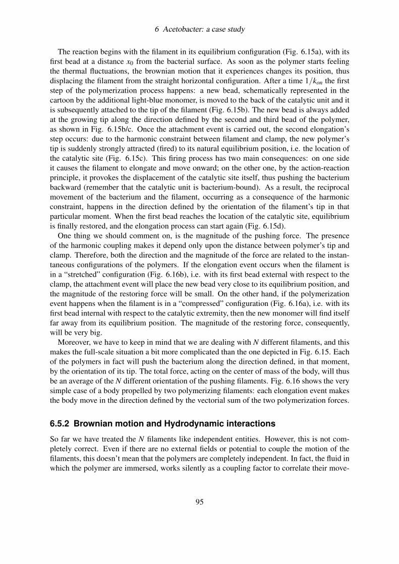
6 Acetobacter: a case study
The reaction begins with the filament in its equilibrium configuration (Fig. 6.15a), with itsfirst bead at a distance x0 from the bacterial surface. As soon as the polymer starts feelingthe thermal fluctuations, the brownian motion that it experiences changes its position, thusdisplacing the filament from the straight horizontal configuration. After a time 1/kon the firststep of the polymerization process happens: a new bead, schematically represented in thecartoon by the additional light-blue monomer, is moved to the back of the catalytic unit and itis subsequently attached to the tip of the filament (Fig. 6.15b). The new bead is always addedat the growing tip along the direction defined by the second and third bead of the polymer,as shown in Fig. 6.15b/c. Once the attachment event is carried out, the second elongation’sstep occurs: due to the harmonic constraint between filament and clamp, the new polymer’stip is suddenly strongly attracted (fired) to its natural equilibrium position, i.e. the location ofthe catalytic site (Fig. 6.15c). This firing process has two main consequences: on one sideit causes the filament to elongate and move onward; on the other one, by the action-reactionprinciple, it provokes the displacement of the catalytic site itself, thus pushing the bacteriumbackward (remember that the catalytic unit is bacterium-bound). As a result, the reciprocalmovement of the bacterium and the filament, occurring as a consequence of the harmonicconstraint, happens in the direction defined by the orientation of the filament’s tip in thatparticular moment. When the first bead reaches the location of the catalytic site, equilibriumis finally restored, and the elongation process can start again (Fig. 6.15d).
One thing we should comment on, is the magnitude of the pushing force. The presenceof the harmonic coupling makes it depend only upon the distance between polymer’s tip andclamp. Therefore, both the direction and the magnitude of the force are related to the instan-taneous configurations of the polymers. If the elongation event occurs when the filament isin a “stretched” configuration (Fig. 6.16b), i.e. with its first bead external with respect to theclamp, the attachment event will place the new bead very close to its equilibrium position, andthe magnitude of the restoring force will be small. On the other hand, if the polymerizationevent happens when the filament is in a “compressed” configuration (Fig. 6.16a), i.e. with itsfirst bead internal with respect to the catalytic extremity, then the new monomer will find itselffar away from its equilibrium position. The magnitude of the restoring force, consequently,will be very big.
Moreover, we have to keep in mind that we are dealing with N different filaments, and thismakes the full-scale situation a bit more complicated than the one depicted in Fig. 6.15. Eachof the polymers in fact will push the bacterium along the direction defined, in that moment,by the orientation of its tip. The total force, acting on the center of mass of the body, will thusbe an average of the N different orientation of the pushing filaments. Fig. 6.16 shows the verysimple case of a body propelled by two polymerizing filaments: each elongation event makesthe body move in the direction defined by the vectorial sum of the two polymerization forces.
6.5.2 Brownian motion and Hydrodynamic interactions
So far we have treated the N filaments like independent entities. However, this is not com-pletely correct. Even if there are no external fields or potential to couple the motion of thefilaments, this doesn’t mean that the polymers are completely independent. In fact, the fluid inwhich the polymer are immersed, works silently as a coupling factor to correlate their move-
95

6 Acetobacter: a case study
ment.Imagine to have a body pushed by one single polymerizing filament. The thermal fluctua-
tions that this filament experiences, make it explore the phase space isotropically. This meansthat the probability to find the polymer’s tip oriented in a certain direction is exactly equalto the probability to find it oriented in the opposite direction. Given that, it is reasonableto believe that on average, one single filament will push the bacterium along the directionperpendicular to the catalytic surface.
How do things change when there are more than one polymerizing chain? Well, in absenceof interactions among filaments, the situation wouldn’t change a lot. Again, on average eachof the filaments will push the body perpendicular to the longitudinal axis of the cell. The totalforce acting on the center of mass of the bacterium will then be the sum of N horizontal forces,and will be horizontal itself. This means that in absence of interactions among filaments, themotion of a body propelled by polymerizing forces is always perpendicular to the longitudinalaxis of the cell, just like intuition suggests (Fig. 6.6).
How then do we explain the motion of A. Xylinum? Well, what really happens in thiscase, is that even in absence of external interactions, like Coulomb or Van der Waals, thepolymers can strongly influence each other just with their presence, through what are calledthe “Hydrodynamic interactions”. Particles, or polymers, immersed in a fluid, excite long-ranged flows as they move, and similarly move in response to fluid motion. By generating andreacting to a fluid’s local velocity, the particles experience hydrodynamic interactions witheach other, that can strongly influence their motion even at relatively large separations.
In this particular case, hydrodynamic interactions couple the elongation process of the Nfilaments. As a result, after an initial transient, the arrangement and the motion of the Npolymers begins to be synchronous, and the directions of the N polymerization forces becomeparallel to each other. Interestingly, this correlation process is so strong that it can coordinatethe buckling transition of the filaments, to break the symmetry of the system and make thebacterium propel in the longitudinal direction. We will describe in detail this phenomenon inthe next section.
6.5.3 Results
Fig. 6.17 shows 6 frames of our Brownian Dynamics simulation. The simulation starts withN = 10 newborn filaments normal to the catalytic surface of the bacterium (Fig.6.17a). Ini-tially, all the strands have the same very short length, and the line that connects the tips ofthe polymers exactly coincides with the row of the catalytic sites. The system is therefore inequilibrium.
When the simulation is turned on, the filaments start to experience the brownian motioncaused by thermal fluctuations, thus shifting from their original equilibrium position. Sincethe first bead of each polymer is harmonically constrained to the catalytic sites, and henceto the bacterium, the motion of the polymers will have repercussion on the bacterial config-uration (Fig.6.17b). With a rate kon, each polymer elongates according to the Load and Firemodel, and while elongating it pushes the bacterium in the direction identified by the instan-taneous orientation of its tip. As you can see from Fig. 6.17, as long as the polymers arevery short, they remain all perpendicular to the catalytic surface, pushing the bacterium in the
96
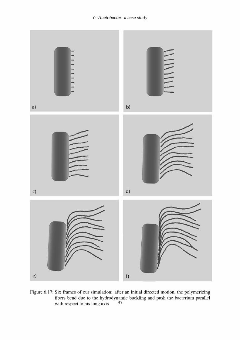
6 Acetobacter: a case study
Figure 6.17: Six frames of our simulation: after an initial directed motion, the polymerizingfibers bend due to the hydrodynamic buckling and push the bacterium parallelwith respect to his long axis 97
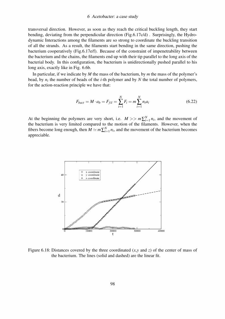
6 Acetobacter: a case study
transversal direction. However, as soon as they reach the critical buckling length, they startbending, deviating from the perpendicular direction (Fig.6.17c/d) . Surprisingly, the Hydro-dynamic Interactions among the filaments are so strong to coordinate the buckling transitionof all the strands. As a result, the filaments start bending in the same direction, pushing thebacterium cooperatively (Fig.6.17e/f). Because of the constraint of impenetrability betweenthe bacterium and the chains, the filaments end up with their tip parallel to the long axis of thebacterial body. In this configuration, the bacterium is unidirectionally pushed parallel to hislong axis, exactly like in Fig. 6.6b.
In particular, if we indicate by M the mass of the bacterium, by m the mass of the polymer’sbead, by ni the number of beads of the i-th polymer and by N the total number of polymers,for the action-reaction principle we have that:
Fbact = M ·ab = Ff il =N
∑i=1
Fi = mN
∑i=1
niai (6.22)
At the beginning the polymers are very short, i.e. M >> m∑Ni=1 ni, and the movement of
the bacterium is very limited compared to the motion of the filaments. However, when thefibers become long enough, then M ' m∑
Ni=1 ni, and the movement of the bacterium becomes
appreciable.
Figure 6.18: Distances covered by the three coordinated (x,y and z) of the center of mass ofthe bacterium. The lines (solid and dashed) are the linear fit.
98
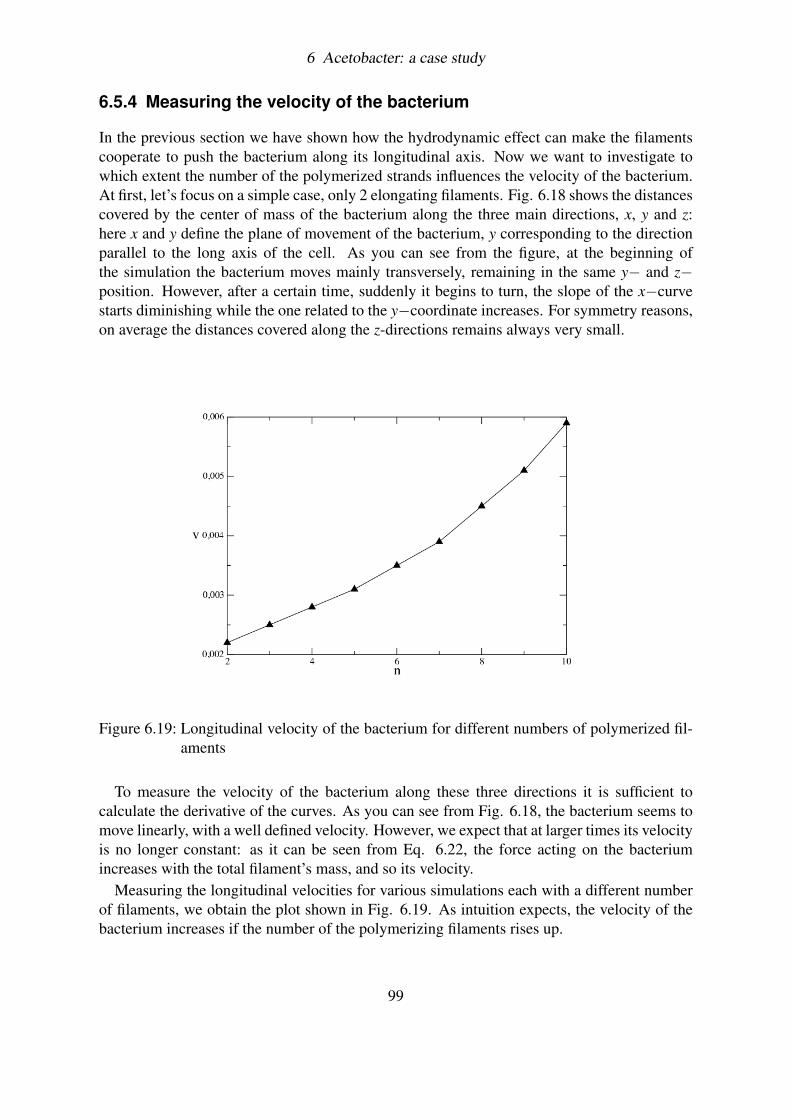
6 Acetobacter: a case study
6.5.4 Measuring the velocity of the bacterium
In the previous section we have shown how the hydrodynamic effect can make the filamentscooperate to push the bacterium along its longitudinal axis. Now we want to investigate towhich extent the number of the polymerized strands influences the velocity of the bacterium.At first, let’s focus on a simple case, only 2 elongating filaments. Fig. 6.18 shows the distancescovered by the center of mass of the bacterium along the three main directions, x, y and z:here x and y define the plane of movement of the bacterium, y corresponding to the directionparallel to the long axis of the cell. As you can see from the figure, at the beginning ofthe simulation the bacterium moves mainly transversely, remaining in the same y− and z−position. However, after a certain time, suddenly it begins to turn, the slope of the x−curvestarts diminishing while the one related to the y−coordinate increases. For symmetry reasons,on average the distances covered along the z-directions remains always very small.
Figure 6.19: Longitudinal velocity of the bacterium for different numbers of polymerized fil-aments
To measure the velocity of the bacterium along these three directions it is sufficient tocalculate the derivative of the curves. As you can see from Fig. 6.18, the bacterium seems tomove linearly, with a well defined velocity. However, we expect that at larger times its velocityis no longer constant: as it can be seen from Eq. 6.22, the force acting on the bacteriumincreases with the total filament’s mass, and so its velocity.
Measuring the longitudinal velocities for various simulations each with a different numberof filaments, we obtain the plot shown in Fig. 6.19. As intuition expects, the velocity of thebacterium increases if the number of the polymerizing filaments rises up.
99
6 Acetobacter: a case study
6.6 Conclusions
In this Chapter we have focused our attention on the bacterium A. Xylinum, a cellulose pro-ducing organism that lives in the air-liquid interface and that exhibits a very peculiar motionduring the cellulose deposition process. We have shown how the symmetry breaking effectoccurring during the bacterial movement is caused by a hydrodynamic coupling between thepolymerized cellulose filaments and the liquid in which they are immersed. To further proveour theory, in the second part of the Chapter we have implemented a Brownian Dynamicssimulation that is able to consistently model the motion of a body immersed in a fluid andpushed by the polymerization forces of elongating polymers. Our numerical simulation hasproved the existence of a symmetry-breaking transition happening during the bacterial motion,and the correlation between the velocity of the bacterium and the number and length of thepolymerized filaments. This suggests the possibility of a quantitative comparison with futureexperiments.
100

7 Appendices
7.1 Appendix A: The Method of Characteristics
The method of characteristics allows to solve the initial value problem for general linear andquasi-linear first order partial differential equations (PDEs). Consider the first order PDE
a(x, t,u)∂u(x, t)
∂x+b(x, t,u)
∂u(x, t)∂t
+ c(x, t,u) = 0 (7.1)
in the two variables (x, t), along with the initial condition
u(x,0) = f (x). (7.2)
The goal of the method of characteristics is to solve the given PDE by finding curves in thex− t plane that reduce the equation to a simple ODE.In general, any curve in the x− t plane can be expressed in parametric form as:
x = x(s)t = t(s)
(7.3)
where the variable s gives a measure of the distance along the curve. In order to label differentcurves in the x− t plane we need to introduce the parameter p such that
x(s = 0) = pt(s = 0) = 0.
(7.4)
The variable p thus identifies the initial point of the curve and it is constant along it. Thisprocedure allows us to change the coordinates from (x, t) to (p,s). In this new coordinatesystem the PDE becomes an ordinary differential equation (ODE) along the generic curve[x(s), t(s)] : 0 < s < ∞, that is called the characteristic curve or just the characteristic.
How do we find the characteristic curves given a generic PDE? Notice that if we choosedxds
= a(x, t,u)
dtds
= b(x, t,u)(7.5)
then we haveduds
=dxds
∂u∂x
+dtds
∂u∂t
= a(x, t,u)∂u∂x
+b(x, t,u)∂u∂t
(7.6)
101
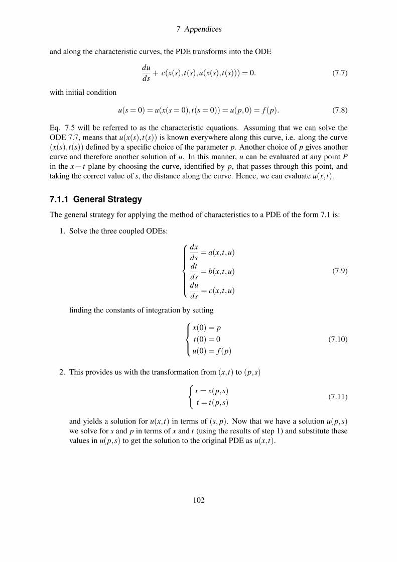
7 Appendices
and along the characteristic curves, the PDE transforms into the ODE
duds
+ c(x(s), t(s),u(x(s), t(s))) = 0. (7.7)
with initial condition
u(s = 0) = u(x(s = 0), t(s = 0)) = u(p,0) = f (p). (7.8)
Eq. 7.5 will be referred to as the characteristic equations. Assuming that we can solve theODE 7.7, means that u(x(s), t(s)) is known everywhere along this curve, i.e. along the curve(x(s), t(s)) defined by a specific choice of the parameter p. Another choice of p gives anothercurve and therefore another solution of u. In this manner, u can be evaluated at any point Pin the x− t plane by choosing the curve, identified by p, that passes through this point, andtaking the correct value of s, the distance along the curve. Hence, we can evaluate u(x, t).
7.1.1 General Strategy
The general strategy for applying the method of characteristics to a PDE of the form 7.1 is:
1. Solve the three coupled ODEs:
dxds
= a(x, t,u)
dtds
= b(x, t,u)
duds
= c(x, t,u)
(7.9)
finding the constants of integration by settingx(0) = pt(0) = 0u(0) = f (p)
(7.10)
2. This provides us with the transformation from (x, t) to (p,s)x = x(p,s)t = t(p,s)
(7.11)
and yields a solution for u(x, t) in terms of (s, p). Now that we have a solution u(p,s)we solve for s and p in terms of x and t (using the results of step 1) and substitute thesevalues in u(p,s) to get the solution to the original PDE as u(x, t).
102

7 Appendices
7.2 Appendix B: Brownian Dynamics
The Brownian Dynamics (BD) simulation technique (108; 109) is a mesoscopic method inwhich explicit solvent molecules are replaced instead by a stochastic force. The techniquetakes advantage of the fact that there is a large separation in time scales between the rapidmotion of solvent molecules and the more sluggish motion of polymers or colloids. The abilityto coarse-grain out these fast modes of the solvent allows one to simulate much larger timescales than in a molecular dynamics simulation. At the core of a BD simulation is a stochasticdifferential equation which is integrated forward in time to create trajectories of molecules.Time enters naturally into the scheme allowing for the study of the temporal evolution anddynamics of complex fluids (e.g. polymers, large proteins, DNA molecules and colloidalsolutions). Hydrodynamic and body forces, such as magnetic or electric fields, can be addedin a straightforward way. BD simulations are particularly well suited to studying the structureand rheology of complex fluids in hydrodynamic flows and other non-equilibrium situations.In the next sections we begin by recovering the theoretical governing stochastic equation, andsubsequently we discretize it and implement it in a BD algorithm.
7.2.1 The Langevin Equation
The BD method is used to describe the dynamics of particles, usually colloids or macro-molecules, that undergo Brownian motion in a viscous solvent. Because of their small mass,inertia is essentially irrelevant for these particles, and it is often neglected in the equation ofmotion. From Newton’s Second Law, Ftot = ma, we see that the neglect of inertia means thatthe total force acting on the particle is always approximately zero. This force is generally com-posed of three terms: a drag force Fd , representing the effect of the viscous solvent throughwhich the particle is moving; a Brownian force FB due to the random collisions of the solventwith the particle; and a last contribution Fnh that includes all the other non-hydrodynamicforces that can be present in the system, such as external body forces, spring forces, and ex-cluded volume interactions.For what has just been said, we therefore have that for the particle i:
Ftoti = Fd
i +FBi +Fnh
i ' 0. (7.12)
Let’s start considering the case of N non-interacting particles in a fluid. In creeping flows(flows with no inertia) and in absence of hydrodynamic interactions (free-draining case), thedrag force is taken as the Stokes drag on a sphere
Fdi =−ζ
(dri
dt
)(7.13)
where ζ = (6πηa), being a the radius of the particle and η the viscosity of the fluid, is the dragcoefficient. The differential equation governing the motion of the particle then becomes
dri
dt=
1ζ(Fnh
i (r j)+FBi (t)) (7.14)
103
7 Appendices
and is commonly called the Langevin equation. Note that in this relation the non-hydrodynamicforce depends on the set of all particle positions r j, while the hydrodynamic drag is takenas a constant for all the particles. Eq. (7.14) is a stochastic differential equation, becausethe Brownian force that act on the particle is extracted from a random distribution. In orderfor the dynamics to satisfy the fluctuation-dissipation theorem, the expectation values of theBrownian force must be
< FBi (t) > = 0 (7.15)
< FBi (t)FB
j (t′) > = 2kBT ζδi jδ(t− t ′)I (7.16)
where kB is the Boltzmann’s constant, T is the absolute temperature, δi j is the Kronecker delta,δ(t− t ′) is the Dirac delta function, and I is the unit second-order tensor. Recalling now theEinstein relation
D =kbT
ζ(7.17)
that relates the thermal motion of the particle, characterized by the diffusion coefficient D,with its response to an external force, we can rewrite the Langevin Equation Eq. (7.14) in themore convenient form:
dri
dt=
DkbT
Fnhi (r j)+
√2D ξi(t) (7.18)
where ξi(t) is a vector with components extracted from a Gaussian distribution, with averageand variance
< ξi(t) > = 0 (7.19)< ξi(t)ξ j(t ′) > = δi jδ(t− t ′)I. (7.20)
Eqs. (7.14), (7.15) and (7.16) are equivalent to the Fokker-Plank equation description, whichis a diffusion equation for the phase-space probability density (110).
7.2.2 Adding Hydrodynamic Interactions
Although the Langevin dynamics correctly describes the behaviour of a single particle (orequivalently of N non-interacting particles) immersed in a fluid, it doesn’t take into accountthe effect caused in the solvent by the presence of other molecules. As a particle movesalong its trajectory, in fact, it exerts a force on the fluid which changes the velocity field fromits undisturbed value. The disturbance velocity changes in its turn the viscous drag forceexerted on the other particles. These interaction effects, mediated by the solvent, are calledhydrodynamic interactions (HI). As a result, the diffusion coefficient of the particles is nolonger a constant (Eq. 7.17), but becomes a configuration-dependent tensor, which will bedenoted by Di j(ri,r j) (110).
The HI are included in the BD through the use of an interaction tensor Ti j, related to thediffusion tensor Di j by the expression
Di j(ri,r j) = kBT Ti j(ri,r j) (7.21)
104
7 Appendices
where the indexes refer to particles i and j. Two interaction tensors are generally used todescribe the hydrodynamic interactions between particles: the Oseen Tensor (111) and theRotne-Prager-Yamakawa tensor (RPY) (112). The first one, whose expression reads like
TOseeni j =
δi jζ
if i = j
18πηri j
(I+ ri jri j
r2i j
)if i 6= j.
is the most known and used. However, it results in a non-positive-definite diffusion tensor ifparticle separations are comparable to the particle radius a. To regularize the singularity inri j = 0, it is possible to use the RPY tensor,
TRPYi j =
δi jζ
if i = j
18πηri j
[(I+ ri jri j
r2i j
)+ 2a2
r2i j
(I3 −
ri jri j
r2i j
)]if i 6= j.
which modifies the small separation behaviour such that the diffusion tensor is always positive-definite. In analogy with Eq. (7.18), the stochastic differential equation including HI thenbecomes
dri
dt=
1kBT
N
∑j=1
Di j(ri,r j) ·Fnhj (rk)+
√2
N
∑j=1
Bi j(rk) ·ξ j(t) (7.22)
where, again, the ξ j are random vectors with expectation values given by Eqs. (7.19) and(7.20). The weighting factors Bi j that appear in Eq. (7.22) must be calculated from thediffusion tensor in order to satisfy the fluctuation-dissipation theorem
Di j(ri,r j) =N
∑p=1
Bip(rk) ·BTjp(rk). (7.23)
This relation can be inverted to calculate the Bi j by Cholesky decomposition. However, amore efficient method has been developed and implemented in BD simulations (108; 109),and will be shown in the next section.
7.2.3 Simulation technique
A BD simulation is performed by integrating the governing stochastic differential equation,(Eq. 7.22), forward in time: the trajectories of the particles in the configuration space arecalculated numerically, and are composed of successive displacements each taken over a shorttime step ∆t. Numerical accuracy limits the maximum size of the time step, requiring it tobe sufficiently short so that the force on the particles and the gradient of the diffusion tensorare essentially constant during ∆t. The stochastic nature of Eq. (7.22) implies that one has toproduce many independent trajectories, that will be subsequently averaged together, to obtainthe time-evolution of an ensemble-averaged observable.
105
7 Appendices
To simulate the diffusion of N identical interacting Brownian particles, we have to rewritethe displacement equation (7.22) in its discretized form as
ri = r0i +
1kbT
N
∑j=1
D0i j ·F0
j ∆t +Ri(∆t) (7.24)
where the subscript 0 indicates that the variable has to be evaluated at the beginning of thetime-step, the term F0
j includes all the non-hydrodynamic forces acting on the particle j (forconvenience we have dropped the superscript nh), and Ri(∆t) represents the effect of the Brow-nian force. The Ri vectors are configuration-dependent, and are composed of Gaussian randomnumbers such that their average and variance are given by
< Ri(∆t) > = 0 (7.25)< Ri(∆t)R j(∆t) > = 2D0
i j∆t. (7.26)
To determine the components of these vectors without inverting Eq. (7.23), we should proceedin the following way (108; 109): let R denote the 3N×1 column vector obtained by stackingthe N Ri column vectors (3×1) on top of each other. Then we can write
R = σ ·X (7.27)
where σ is a configuration dependent 3N × 3N matrix and X is a 3N × 1 column vector ofnormally distributed Gaussian random numbers
< Xm > = 0 (7.28)< XmXn > = 2δmn∆t (7.29)
obtained from a random number generator. If we let Q denote the symmetric 3N×3N super-matrix constructed form the Di j matrices in the following manner
Q =
D11 D12 ... D1ND21 D22 ... D2N... ... ... ...
DN1 DN2 ... DNN
then the elements of σ are simply given by
σmm =
(Qmm−
m−1
∑k=1
σ2mk
)1/2
(7.30)
σmn =
(Qmn−∑
n−1k=1 σmkσnk
)σnn
. (7.31)
106
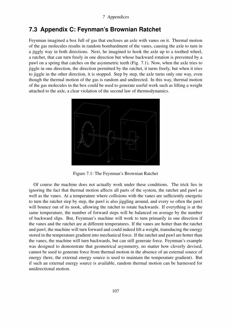
7 Appendices
7.3 Appendix C: Feynman’s Brownian Ratchet
Feynman imagined a box full of gas that encloses an axle with vanes on it. Thermal motionof the gas molecules results in random bombardment of the vanes, causing the axle to turn ina jiggly way in both directions. Next, he imagined to hook the axle up to a toothed wheel,a ratchet, that can turn freely in one direction but whose backward rotation is prevented by apawl on a spring that catches on the asymmetric teeth (Fig. 7.1). Now, when the axle tries tojiggle in one direction, the direction permitted by the ratchet, it turns freely, but when it triesto jiggle in the other direction, it is stopped. Step by step, the axle turns only one way, eventhough the thermal motion of the gas is random and undirected. In this way, thermal motionof the gas molecules in the box could be used to generate useful work such as lifting a weightattached to the axle, a clear violation of the second law of thermodynamics.
Figure 7.1: The Feynman’s Brownian Ratchet
Of course the machine does not actually work under these conditions. The trick lies inignoring the fact that thermal motion affects all parts of the system, the ratchet and pawl aswell as the vanes. At a temperature where collisions with the vanes are sufficiently energeticto turn the ratchet step by step, the pawl is also jiggling around, and every so often the pawlwill bounce out of its nook, allowing the ratchet to rotate backwards. If everything is at thesame temperature, the number of forward steps will be balanced on average by the numberof backward slips. But, Feynman’s machine will work to turn primarily in one direction ifthe vanes and the ratchet are at different temperatures. If the vanes are hotter than the ratchetand pawl, the machine will turn forward and could indeed lift a weight, transducing the energystored in the temperature gradient into mechanical force. If the ratchet and pawl are hotter thanthe vanes, the machine will turn backwards, but can still generate force. Feynman’s examplewas designed to demonstrate that geometrical asymmetry, no matter how cleverly devised,cannot be used to generate force from thermal motion in the absence of an external source ofenergy (here, the external energy source is used to maintain the temperature gradient). Butif such an external energy source is available, random thermal motion can be harnessed forunidirectional motion.
107


Bibliography
[1] M. R. Brown, Jr. Journal of Plymer Science, 42:487–495, 2004.
[2] B. G. Ranby. Acta Chem. Scand., 6:128, 1952.
[3] S. Kuga and Jr. M. R. Brown. Carbohydrate Res., 180:345, 1988.
[4] Helbert W. Amai T. Sugiyama J. Koyama, M. and B. Henrissat. Proc. Natl. Acad. Sci.USA, 94:9091, 1997.
[5] R. Atalla and D. L. VanderHart. Science, 223:283–285, 1984.
[6] Sugiyama J. Wada, M. and T. Okano. J. App. Polymer Sci., 49:1491, 1993.
[7] Persson J. Sugiyama, J. and H. Chanzy. Macromolecules, 24:2461–2466, 1991.
[8] S. Kimura and T. Itoh. Protoplasma, 194:151, 1996.
[9] Takagi S. Kuga, S. and M. R. Brown Jr. Polymer, 34:3293–3297, 1993.
[10] Togawa E. Kondo, T. and Jr. M. B. Brown. Biomacromolecules, 2:1324–1330, 2001.
[11] M. Benziman, C. H. Haigler, R. M. Brown Jr., A. R. White, and K. M. Cooper. Proc.Natl. Acad. Sci. USA, 77:6678–6682, 1980.
[12] Brown R. M. Jr. Haigler, C. H. and M. Benziman. Science, 210:903, 1980.
[13] S. K. Cousins and R. M. Brown Jr. Polymer, 36:3885–3888, 1995.
[14] S. Cousins and Jr. M. R. Brown. Polymer, 38:903, 1997.
[15] R. D. Preston. In Zimmerman M.H., ed. Formation of Wood in Forest Trees, New York,Academic Press:169–188, 1964.
[16] S. C. Mueller and R. M. Brown Jr. J. Cell Biol., 84:315–326, 1980.
[17] S. Kimura, W. Laosinchai, T. Itoh, K. Cui, C. R. Linder, and R. M. Brown Jr. The PlantCell, 11:2075–2085, 1999.
[18] R. M. Brown Jr., J. H. M. Willison, and C. L. Richardson. Proc. Natl. Acad. Sci. USA,73(12):4565–4569, 1976.
[19] Ohshima C . Hirose E . Nishikawa J . Itoh T . Kimura, S . Protoplasma, 216:71–74,2001.
109
Bibliography
[20] H. Peng and L. Jaffe. Planta, 133:57–71, 1976.
[21] M. R. Jr. Brown. Pure Appl. Chem., 10:1345–1373, 1996.
[22] D. P. Delmer. Annu. Rev. Plant. Physiol. Plant. Mol. Biol., 50:245–276, 1999.
[23] I. Tsekos. J.Phycol, 35:635–655, 1999.
[24] J. H. M. Willison and Jr. M. R. Brown. Planta, 141:51–58, 1978.
[25] I. Tsekos and H. Reiss. Protoplasma, 169:57–67, 1992.
[26] R. M. Jr. Itoh, T. Brown. Planta, 160:372–381, 1984.
[27] S. Mizuta and R. M. Jr. Brown. Protoplasma, 166:187–199, 1992.
[28] Roberts E. M. Mizuta, S. and R. M. Jr. Brown. Cellulose and wood: Chemistry andTechnology, Wiley, New York, ed. C. Schuerch:659–676, 1989.
[29] Brower D. L. Giddings, T. H. Jr. and L. A. Staehelin. J. Cell. Biol., 84(2):327–339,1980.
[30] C. R. Woese. Microbiol. Rev., 51:221–271, 1987.
[31] Oyaizu Y. Oyaizu H. Olsen G. J. Yang, D. and C. R. Woese. Proc. Natl. Acad. Sci. USA,82:4443, 1985.
[32] M. H. Deinema and L. P. T. M. Zevenhuizen. Arch. Mikrobiol., 78:42–57, 1971.
[33] Mayer R. Ross, P. and M. Benziman. Microbiol. Mol. Biol. Rev., 55:35–58, 1991.
[34] Rohde M. Bokranz W.and Ro Zogaj X., Nimtz M. Mol. Microbiol., 39:1452–1463,2001.
[35] E. Roberts. Biosynthesis of cellulose II and related carbohydrates. PhD thesis., pagesUniversity of Texas, Austin, 1991.
[36] Fuller D. Iranfar N. Grimson M. J. Blanton, R. L. and W. F. Loomis.Proc.Natl.Acad.Sci.USA, 97:2391–2396, 2000.
[37] Haigler C. H. Grimson, M. J. and R. Blanton. J. Cell. Science, 109:3079–3087, 1996.
[38] S. Kimura and T. Itoh. Cellulose, 11:377–383, 2004.
[39] Jr. R. M. Brown. Journal of Cell Science Suppl., 2:13–32, 1985.
[40] Kawagoe Y. Schreckengost W. E. Delmer D. P. Stalker D. M. Pear, J. R. Proc. Natl.Acad. Sci. USA, 93:12637–12642, 1996.
110
Bibliography
[41] T. Arioli, L. Peng, A.S. Betzner, J. Burn, W. Wittke, W. Herth, C. Camilleri, H. Höfte,J. Plazinski, R. Birch, A. Cork, J. Glover, J. Redmond, and R. E. Williamson. Science,279:717–720, 1998.
[42] T.A. Richmond and C.R. Somerville. Plant Physiol., 124:445–448, 2000.
[43] Somerville C. R. Turner, S. R. Plant Cell, 9:689–701, 1997.
[44] Scheible W. R. Cutler S. Somerville C. R. Taylor, N. G. and S. R. Turner. Plant Cell,11:769–780, 1999.
[45] Howells R. M. Huttly A. K. Vickers K . Turner S. R. Taylor, N. G. Proc. NAtl. Acad.Sci. USA, 100:1450–1455, 2003.
[46] Mouille G. Robert, S. and H. Hofte. Cellulose, 11:351–364, 2004.
[47] Taylor N.G. Gardiner, J.C. and S.R. Turner. Plant Cell, 15:1740–1748, 2003.
[48] Eshed R. Richmond T. Delmer D. Scheible, W. R. and Somerville C. Proc. Natl. Acad.Sci. USA, 98:10079–10084, 2001.
[49] Kurek I. Jacob-Wilk D. Doblin, M. S. and D.P. Delmer. Plant Cell Physiol., 43:1407–1420, 2002.
[50] A. M. C. Emons and A. M. C. Wolters-Arts. Protoplasma, 117:68–81, 1983.
[51] N. C. Carpita and D. M. Gibeaut. Plant J., 3:1–30, 1993.
[52] M. C. McCann and K. Roberts. J. Plant Sci., 96:323–334, 1990.
[53] A. Mogilner and G. Oster. Curr. Biology, 13:R721–R733, 2003.
[54] C. C. Peskin, G. M. Odell, and G. Oster. Biophys. J., 65:316–324, 1993.
[55] A. Bowling and R. M. Brown Jr. 2005. http://www.botany.utexas.edu/facstaff/-facpages/mbrown/bowling/default2.html.
[56] A. M. C. Emons. Planta, 163:350–359, 1985.
[57] R. M. Brown Jr. Pure Appl. Chem., 71:765–775, 1999.
[58] R. M. Brown Jr. and D. Montezinos. Proc. Natl. Acad. Sci. USA, 80:773–777, 1976.
[59] A. R. Paredez, C. R. Somerville, and D. W. Erhardt. Science, 312:1491, 2006.
[60] F. Jülicher, A. Ajadari, and J. Prost. RPM Colloquia, 69:1269–1281, 1997.
[61] I. B. Heath. J. Theor. Biol., 48:445–449, 1974.
[62] P. K. Hepler and B. A. Palevitz. Annu. Rev. Plant. Physiol., 25:309–362, 1974.
111

Bibliography
[63] W. Herth. J. Cell Biol., 87:442–450, 1980.
[64] A. Mogliner and G. Oster. Biophys. J., 71:3030, 1996.
[65] Leighton R. B. Feynman, R. P. and M. Sands. The Feynman lectures on Physics, 1.USA, Addison-Wesley:46.1–46.9, 1963.
[66] R.D. Astumian. Science, 276:917–922, 1997.
[67] T. L. Hill and M.W. Kirschner. Int. Rev Cytol, 78:1–125, 1982.
[68] A. M. C. Emons. In C. H. eds. Haigler and P. J. Weimer, editors, Biosynthesis andBiodegradation of Cellulose, pages 71–98. Marcel Dekker, New York, 1991.
[69] D. R. Daniels and M. S. Turner. J. Chem. Phys, 121:7401–7407, 2004.
[70] S. J. Eichhorn and R. J. Young. Cellulose, 8:197–207, 2001.
[71] C. H. Haigler and M. Benziman. Cellulose and Other Natural Polymer Systems,R.M.Brown Jr. ed., New York, Plenum Press:273–297, 1982.
[72] N. Hirai, S. Senobe, and T. Hayashi. Proc. Natl. Acad. Sci. USA, 95:15102–15106,1998.
[73] S. A. Safran. Statistical Thermodynamics of Surfaces, Interfaces, and Membranes.Addison-Wesley, Reading MA, 1994.
[74] I. Derenyi, F. Jülicher, and J. Prost. PRL, 88:238101, 2002.
[75] G. C. Ruben and G. H. Bokelman. Carbohydate Research, 160:434–443, 1986.
[76] S. J. Hanley, J. F. Revol, L. Godbout, and D. G. Gray. Cellulose, 4:209–220, 1997.
[77] P. H. Raven, R. F. Evert, and S. E. Eichhorn. Biology of Plants. W. H. Freeman, NewYork, 6th edition, 1999. pp. 66-67.
[78] A. M. C. Emons and B. M. Mulder. Proc. Natl. Acad. Sci. USA, 95:7215–7219, 1997.
[79] T.I. Baskin. Protoplasma, 215:150–171, 2001.
[80] K. Roberts. The plant extracellular matrix. Curr. Opinion Cell Biol., 5:1020–1027,1989.
[81] A. M. C. Emons and B. M. Mulder. Plant cell wall architecture. Comm. Theor. Biol., 4:115–131, 1997.
[82] D. Reis, J. C. Roland, and B. Vian. Morphogenesis of twisted cell wall: chronologyfollowing an osmotic shock. Protoplasma, 126:36–46, 1985.
[83] A.C. Neville. Biology of fibrous composites: Development beyond the cell membrane.Cambridge University Press, 1993.
112
Bibliography
[84] Saxena I. M. Brown, Jr. R. M. and K. Kudlicka. Trends in Plant Science, 1:149–156,1996.
[85] C Wymer and C Lloyd. Dynamic microtubules: implications for cell wall patterns.Trends Plant Sci., 1:222–228, 1996.
[86] A. M. C. Emons, J. Derksen, and M. M. A. Sassen. Physiol. Plant, 84:486–493, 1992.
[87] A.M.C. Emons. Winding threads around plant cells: a geometrical model for microfibrildeposition. Plant Cell and Environment, 17:3–14, 1994.
[88] B. M. Mulder and A. M. C. Emons. A dynamical model for plant cell wall deposition.J. Math. Biol., 42:261–289, 2001.
[89] N. C. A. De Ruijter, M. B. Rook, T. Bisseling, and A. M. C. Emons. Lipochito-oligosaccharides re-initiate root hair tip growth in vicia sativa with high calcium andspectrin-like antigen at the tip. Plant J., 13:341–350, 1999.
[90] H. R. Petty, R. G. Worth, and A. L. Kindzelskii. Imaging sustained dissipative patternsin the metabolism of individual living cells. Phys. Rev. Lett., 84:2754–2757, 2000.
[91] A. M. C. Emons. Acta Bot. Neerl., 37:31–38, 1988.
[92] A. J. Brown. J. Chem. soc., 49:432–439, 1886.
[93] A. J. Brown. J. Chem. soc., 51:643, 1887.
[94] Dutta D. and R. Gachhui. Int J Syst Evol Microbiol, 56:1899–1903, 2006.
[95] COUPERWHITE I. BERNARDO E. B., NEILAN B. A. Syst. appl. microbiol., 21:599–608, 1998.
[96] S. Schramm, M. Hestrin. J. Gen. Microbiol., 11:123, 1954.
[97] Kjosbakken J. Valla, S. ibid., 128:1401–1408, 1982.
[98] Cannon R. E. William W., S. Appl. Env. Microbiol., 55:2448, 1989.
[99] Yamanaka S. Budhiono A. Iguchi, M. J. Material Science, 34:261–270, 2000.
[100] M. Benziman and H. Burger-Rachamimov. J Bacteriol., 84:625–630, 1962.
[101] H. Weinhouse and M. Beriman. Biochem. J., 138:537–542, 1974.
[102] White A. R. Brown M. B. Jr. Haigler, C. H. and K. M. Cooper. J. Cell Biology, 94:64–69, 1982.
[103] Saito M. Kuga S. Shibazaki, H. and T. Okano. Cellulose.
[104] Tsuji M Hirai, A. and F. Horii. Cellulose, 9:105–113, 2002.
113

Bibliography
[105] G. K. Batchelor. J. Fluid. Mech., 44:410, 1970.
[106] Julicher F. Camalet, S. New Journal of Physics, 24:1–23, 2000.
[107] Kruiskamp P. H. Vliegenthart J. F. G. Kroon Kroon-Batemburg, L. M. J. J. Phys. ChemB, 101:8454–8459, 1997.
[108] D. L. Ermak and J. A.. McAmmon. J. Chem. Phys., 69(4):1352–1360, 1978.
[109] S.A. Allison and J. A. McAmmon. Biopolymers, 23:167–187, 1984.
[110] H. C. Ottinger. Stochastic processes in polymeric fluids. Springler-Verlag, New-York,1996.
[111] M. Doi and S. F. Edwards. The theory of polymer dynamics. Oxford Science Publica-tions, New-York, 1986.
[112] S. Rotne, J.and Prager. J. Stat. Phys., 14:153, 1976.
114
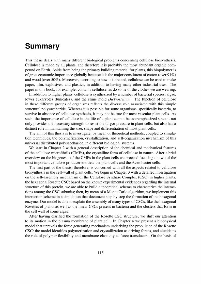
Summary
This thesis deals with many different biological problems concerning cellulose biosynthesis.Cellulose is made by all plants, and therefore it is probably the most abundant organic com-pound on Earth. Aside from being the primary building material for plants, this biopolymer isof great economic importance globally because it is the major constituent of cotton (over 94%)and wood (over 50%). Moreover, according to how it is treated, cellulose can be used to makepaper, film, explosives, and plastics, in addition to having many other industrial uses. Thepaper in this book, for example, contains cellulose, as do some of the clothes we are wearing.
In addition to higher plants, cellulose is synthesized by a number of bacterial species, algae,lower eukaryotes (tunicates), and the slime mold Dictyostelium. The function of cellulosein these different groups of organisms reflects the diverse role associated with this simplestructural polysaccharide. Whereas it is possible for some organisms, specifically bacteria, tosurvive in absence of cellulose synthesis, it may not be true for most vascular plant cells. Assuch, the importance of cellulose in the life of a plant cannot be overemphasized since it notonly provides the necessary strength to resist the turgor pressure in plant cells, but also has adistinct role in maintaining the size, shape and differentiation of most plant cells.
The aim of this thesis is to investigate, by mean of theoretical methods, coupled to simula-tion techniques, the polymerization, crystallization, and self-organization mechanism of thisuniversal distributed polysaccharide, in different biological systems.
We start in Chapter 2 with a general description of the chemical and mechanical featuresof the cellulose microfibrils (CMFs), the crystalline form of cellulose in nature. After a briefoverview on the biogenesis of the CMFs in the plant cells we proceed focusing on two of themost important cellulose producer entities: the plant cells and the Acetobacter cells.
The first part of the thesis, therefore, is concerned with all the aspects related to cellulosebiosynthesis in the cell-wall of plant cells. We begin in Chapter 3 with a detailed investigationon the self-assembly mechanism of the Cellulose Synthase Complex (CSC) in higher plants,the hexagonal Rosette CSC: based on the known experimental evidences regarding the internalstructure of this protein, we are able to build a theoretical scheme to characterize the interac-tions among the CSC subunits; then, by mean of a Monte Carlo algorithm, we implement thisinteraction scheme in a simulation that document step by step the formation of the hexagonalenzyme. Our model is able to explain the assembly of many types of CSCs, like the hexagonalRosettes of plants as well as the linear CSCs present in bacteria and the clusters that form inthe cell wall of some algae.
After having clarified the formation of the Rosette CSC structure, we shift our attentionto its motion in the plasma membrane of plant cell. In Chapter 4 we present a biophysicalmodel that unravels the force generating mechanism underlying the propulsion of the RosetteCSC: the model identifies polymerization and crystallization as driving forces, and elucidatesthe role of polymer flexibility and membrane elasticity as force transducers. On the basis of
115
Summary
our model and appropriate values for the relevant physical constants, we obtain a theoreticalestimate for the velocity of the CSC that is in agreement with the experimental value. To havea proof a principle of the proposed mechanism, we have also developed a stochastic simulationthat reproduces the movement of the Rosette CSC in the fluid membrane of the plant cell.
The last issue related to plant cells cellulose is the formulation of a mathematical model toanalyze the building of cell wall architecture (Chapter 5). The highly regular textures observedin cell walls reflect the spatial organization of the cellulose CMFs. Based on a geometricalhypothesis proposed earlier, we formulate a model that describes the space-time evolutionof the density of Rosette CSCs in the plasma membrane of plant cell. The trajectories ofthe Rosettes are assumed to be governed by an optimal packing constraint of the CMFs thatcouples the direction of motion to the density of the CSCs. Our model is based on a relativelysmall numbers of variables that can be tuned to obtain most of the cell wall textures that havebeen found experimentally. Moreover, we demonstrate that it is also robust against a numberof perturbations and noise effects.
The second part of the thesis is focused on the cellulose-producing Acetobacter cells, whichlive at the air-liquid interface and which exhibit a peculiar motion during the cellulose poly-merization process. The mechanism of formation as well as the structure of the bacterialcellulose has been studied extensively in recent decades. The cellulose product appears as along ribbon, composed of many CMFs, which extends parallel to the longitudinal axis of thecell, and which is synthesized by a linear array of particles placed along the axis of the bac-terial rod. Goal of this chapter (Chapter 6) is to correlate the peculiar motion of Acetobacterwith an hydrodynamic effect caused by the interactions between the cellulose CMFs and thefluid in which they are immersed. To further assess the correctness of our model, in the lastpart of the thesis we implement a Brownian Dynamics simulation that is able to reproduce themain features of this particular bacterial motion.
116
Samenvatting
Dit proefschrift behandelt verschillende biologische aspecten van de biosynthese van cellu-lose. Cellulose wordt door alle planten gemaakt en is daardoor waarschijnlijk het meestvoorkomende organische polymeer op aarde. Naast een van de belangrijkste bouwstoffenvan planten, is dit polymeer ook wereldwijd van groot economisch belang omdat het een be-langrijke component van katoen (meer dan 94%) en van hout (meer dan 50%) is. Bovendienkan cellulose, afhankelijk van hoe het behandeld wordt, gebruikt worden voor het maken vanpapier, film, explosieven en plastics, naast nog veel andere industriële toepassingen. Hetpapier waarop dit boek gedrukt is, en veel van de kleren die wij dragen, bevatten dan ook veelcellulose.
Naast de hogere planten, produceren ook enkele bacteriesoorten, algen, lagere eukaryotenzoals tunicaten en de slijmschimmel Dictyostelium cellulose. De uiteenlopende functies vancellulose in deze verschillende groepen van organismen, geeft de de heel verschillende rollenaan die dit simpele structurele polysaccheride kan spelen. Daar waar sommige organismenechter kunnen overleven zonder cellulose te produceren, geldt dit niet voor de vaatplanten. Alszodanig kan de rol van cellulose voor het leven van planten dan ook niet overschat worden,aangezien het de benodigde mechanische sterkte levert, die het mogelijk maakt dat planten-cellen de turgordruk weerstaan, en bovendien een belangrijke rol speelt bij het bepalen van devorm, de omvang en de differentiatie van van de meeste plantencellen.
Het doel van dit proefschrift is om met behulp van theoretische beschouwingen gekoppeldaan computersimulaties de polymerisatie, de kristallisatie en de zelforganisatie principes vandit zo universeel verbreide polysacchride te onderzoeken in verschillende biologische syste-men.
We starten in hoofdstuk 2 met een algemene beschrijving van de chemische en mechanischeeigenschappen van Cellulose Microfibrillen (CMFs), de kristallijne vorm waarin het in denatuur voorkomt. Na een kort overzicht van de biogenese van de CMFs, richten wij onsop de twee meest prominente cellulose producerende organismen, planten en Acetobacterbacteriën.
Het eerste deel van het proefschrift gaat daarom over alle aspecten van de biosynthese vancellulose in de celwanden van planten. We starten in hoofdstuk 3 met een gedetailleerdebeschrijving van het zelfassemblage proces van het Cellulose Synthase Complex (CSC) inhogere planten, het hexagonale eiwitcomplex dat ook wel “Rosette” wordt genoemd. Gebaseerdop de bestaande experimentele aanwijzingen omtrent de interne structuur van dit eiwitcom-plex, zijn we in staat een theoretisch model op te stellen voor de interacties tussen de subeen-heden van het CSC. Vervolgens implementeren we deze interacties in een Monte Carlo sim-ulatie, die de stap voor stap assemblage van het hexagonale enzymcomplex in beeld brengt.Ons model is in staat om de constructie van veel verschillende types van CSCs te beschrijven,niet alleen de hexagonale Rosettes zoals die in planten worden gevonden, maar ook the lin-
117
Samenvatting
eaire CSCs van sommige bacteriesoorten en de clusters zoals die in de celwand van sommigealgen voorkomen.
Na de vorming van de structuur van het Rosette CSC te hebben opgehelderd, richten wij onsop zijn beweging in het plasmamembraan van de cel. In hoofdstuk 4 presenteren wij een biofy-sisch model dat het krachten productie mechanisme dat ten grondslag ligt aan de voortstuwingvan het Rosette CSC ontrafelt. Het model identificeert de polymerisatie en de kristallisatie vande cellulose as drijvende krachten, en geeft opheldering over de rol van polymeerflexibiliteiten membraan elasticiteit in het overbrengen van deze krachten. Op basis van ons model en dewaarden van de relevante fysische constanten geven wij een schatting van de snelheid van hetCSC die in goede overeenstemming is met de experimentele waarde. Om het principe achterons model verder te testen, ontwikkelden we een stochastische simulatie die de beweging vanhet CSC in het membraan van de plantencel reproduceert.
Het laatste thema rond cellulose in planten cellen, is een mathematisch model voor hetbeschrijven van de bouw van de architectuur van planten celwanden (hoofdstuk 5). De zeerregelmatige texturen van planten celwanden, reflecteert de ruimtelijke organisatie van de CMFs.Gebaseerd op een eerder geformuleerde geometrische hypothese, stellen wij een model op datde ruimte-tijd evolutie van de dichtheid van Rosette CSCs in het plasmamembraan beschrijft.De baenen van de CSCs worden bepaald door een optimale pakkingvoorwaarde die de be-wegingsrichting koppelt aan de dichtheid van de CSCs. Het model heeft slechts een beperktaantal parameters, die zo gekozen kunnen worden dat de meest van de experimenteel gevon-den celwand texturen gereproduceerd worden. We laten bovendien zien dat het model robuustis tegen een aantal verstoringen en de effecten van ruis.
Het tweede deel van het proefschrift richt zich op de cellulose producerende Acebactercellen, bacteriën die leven aan het lucht-water grensvlak en die een merkwaardige bewegingvertonen gedurende het cellulose polymerisatieproces. Het vormingsproces en de structuurvan is intensief bestudeerd de afgelopen decennia. Het cellulose product verschijnt als eenlanggerekt lint, samengesteld uit vele CMFs, dat zich strekt in de richting parallel aan delange as van de cel, en dat gesynthetiseerd wordt door een lineaire reeks van deeltjes langs deas van de staafvormige bacterie. Het doel van hoofdstuk 6 is om het bewegingsmechanismevan Acetobacter in verband te brengen met een hydrodynamisch effect dat ontstaat door dewisselwerking van de CMFs en het vloeibare medium waarin zij ondergedompeld zijn. Om dejuistheid van dit principe te testen, implementeren wij in het laatste deel van het proefschrifteen Brownse Dynamica simulatie, die in staat blijkt de voornaamste kenmerken van dezeaparte vorm van bacteriële voortbeweging te reproduceren.
118
List of Publications
The work in this thesis covers the following pubblications:
Chapter 5:The Cellulose Synthase Complex: a polymerization driven supramolecular motor(Biophys J. 2007 Apr 15;92(8):2666-73.)Diotallevi F., Mulder, B.
Chapter 4:The dynamics of interacting comoving CMF synthases,(in preparation)Diotallevi F., Mulder, B.
Chapter 6:Hydrodynamic buckling drives the motion of A. Xylinum,(in preparation)Diotallevi F., Mulder, B., Joanny, J.F.
Chapter 3:A model for the assembly of the CSC in plant cells,(in preparation)Diotallevi F., Mulder, B.
Other pubblications:
Capillary filling using Lattice Boltzmann Equations: the case of multi-phase flows ,(submitted to EPJ)F. Diotallevi, L. Biferale, S. Chibbaro, A. Lamura G. Pontrelli, M. Sbragaglia, S. Succi, F.Toschi
Fluid-like behavior of a one-dimensional granular gas,(J. Chem. Phys. 120(1) 35 ( 2004))F. Diotallevi, U. Marini Bettolo Marconi, A. Puglisi, F. Cecconi
Inelastic hard-rods in a periodic potential,(J. Chem. Phys. 121, 5125 (2004))F. Diotallevi, U. Marini Bettolo Marconi, A. Puglisi, F. Cecconi

Note added in proof
We are grateful to a member of the reading committee,prof. dr. R. M. Brown Jr, an acknowl-edged world expert on cellulose, who has alerted us to a number of omissions of literaturecitations in the text as well as references to figures used from the literature in the thesis. Un-fortunately, for technical reasons we were not able to redress these in time for submission. Weapologize to any readers that justifiably feel that we have not been comprehensive enough inour referencing and figure attributions, and we assure them that we will address these issuesas fully as possible in future publications.

Acknowledgments
This work would not have been possible without the help and support of a number of people,whom I wish to thank.
First and most of all I want to thank my promotor Bela Mulder, who introduced me to therich and surprising world of cellulose. Besides being a careful and helpful supervisor, Belahas always been patient and tolerant, giving me the possibility to enrich my knowledge on thisresearch subject by mean of various collaborations with different groups and people in manycountries.I also want to express my thanks to Anne Mie Emons, with whom I had the pleasure to workespecially during the initial stage of my PhD. I am grateful to Anne Mie for her helpful advicesand suggestions, and for her kind answers to my numerous questions regarding plant biology.Together with Bela, Daan Frenkel has been my other guiding light: with his deep knowledgeand brilliant ideas Daan was able to find solutions to the most tricky problems, offering me hissupport on innumerable circumstances.I thank Jean Francois Joanny for allowing me to stay for three months in his lab in Paris: thecollaboration with Jean Francois was very useful, and decisive for the work on Acetobacterpresented in Chapter 6.My thanks also go to Giovanni Ciccotti, that hosted me in Rome and taught me all I knowabout MD simulations of polymers in solvent. I hope that the fruit of our collaboration willsee the light in a very soon future.I thank all the Amolfers, especially the "Overloopers", for the interesting discussions that havebeen a continuous source of ideas and enthusiasm.I also give my thanks to Sauro Succi and Luca Biferale, who kindly allowed me to work onthis thesis during the first months of my new job.
Finally, I would like to thank a number of other people that were not directly involved inthe work presented in this Thesis.First, all my friends spread around the world: Netherlands and Italy, England and France,Spain and US and many more countries... It would be impossible to mention all of you (I’msorry for that!), but I’m sure that you know how much you mean and have meant to me, espe-cially during these years abroad, and how important your presence has been in my dark days.Un grazie enorme va alla mia famiglia, che ha (da sempre...) accettato e supportato ogni miadecisione, per quanto folle la potesse trovare. Un grazie particolare va ai miei nonni e alle mienonne, a cui non smetto mai di pensare e a cui questa tesi è dedicata.Much more than a thank you goes to Andrea, who has always been by my side despite thou-sands of kilometres were keeping us apart: mi hai lasciato partire senza mai lasciarmi sola,non lo dimentichero’ mai.
The work described in this thesis was performed at the FOM Institute for Atomic and MolecularPhysics, Kruislaan 407, 1098 SJ, Amsterdam, The Netherlands. The work is part of the researchprogram of the Stichting voor Fundamenteel Onderzoek der Materie (FOM) and was made possible byfinancial support from the Nederlandse Organisatie voor Wetenschappelijk Onderzoek (NWO).
Cover: Revised Ernst Haeckel’s interpretation of several Tunicates (Ascidians), the only animals ableto synthesize cellulose. From Kunstformen der Natur (Artforms of Nature), 1904.

“In Olanda... non capisconon mi sento soddisfatto
sara’ che e’ tutto cosi’ drittocosi’ spietatamente piatto...”
Banalita’, Daniele Silvestri

Education Statement of the Graduate School
Experimental Plant Sciences
Issued to:Date: 26 October 2007Group:
1) Start-up phase date First presentation of your project
Writing or rewriting a project proposal Writing a review or book chapter
Jun 2003 Laboratory use of isotopes
Subtotal Start-up Phase 5.5 credits*
2) Scientific Exposure date EPS PhD student days
26 Apr 200512 May 2006
2003-20062003-2005
KNAW and NWO Biophysics Meetings (4x1 day) 2003-2006
18-19 Nov 20041-2 Dec 2005
Jan 2007 Seminar plus
Soft Condensed Matter Physics- NATO, Edinburgh, UK (9 days) 29 Mar-8 Apr 20041-4 Nov 20055-9 Jun 20069-13 Jul 2007
Presentations20042005
2003-20052006
IAB interview Excursions
Subtotal Scientific Exposure 19.3 credits*
3) In-Depth Studies date EPS courses or other PhD courses
2003-2006 Journal club
Journal Club “Life Inspired Physics Group” 2003-2007 Individual research training
Subtotal In-Depth Studies 7.8 credits*
4) Personal development date Skill training courses
Writing structural English 2004Writing Scientific English 2006
Membership of Board, Committee or PhD council
Subtotal Personal Development 1.8 credits*
TOTAL NUMBER OF CREDIT POINTS* 34.4Herewith the Graduate School declares that the PhD candidate has complied with the educational requirements set by theEducational Committee of EPS which comprises of a minimum total of 30 credits
* A credit represents a normative study load of 28 hours of study
Fabiana Diotallevi
Theory of Biomolecular Matter (AMOLF Institute) &Plant Cell Biology, Wageningen University
Oral presentation: “Understanding Cellulose Biosynthesis”, AMOLF institute Sep 2003
MSc coursesMolsim- Simulation Course (Amsterdam)
EPS PhD Student Day, Wageningen University 19 Sep 2006EPS theme symposiaEPS Theme 1 sympsium 'Developmental Biology of Plants' , Wageningen UniversityEPS Theme 1 sympsium 'Developmental Biology of Plants' , Leiden UniversityNWO Lunteren days and other National PlatformsNWO meetings Lunteren Biophysics (4x2 days)Lunteren Statistical Mechanics (2x2 days)
Seminars (series), workshops and symposiaBiolateral Triangle Meeting, Dresden, Germany (2 days)Biolateral Triangle Meeting, Amsterdam, Netherlands (2 days)Biolateral Triangle Meeting, Paris, France (2 days)
International symposia and congresses
Julich Soft Matter Days, Bonn, Germany (4 days)Sitges Conference, Barcelona, Spain (5 days)StatPhys Conference, Genova, Italy (5 days)
Biolateral Triangle Meeting, Dresden, Germany EPS- Theme SymposiaLunteren Poster Session (3x)Sitges Conference, Poster session
19 Sep 2006
VU-Amolf Complex System Summerschool (4x4days)
Organisation of PhD students day, course or conference