Embed Size (px)
Citation preview

Munich Personal RePEc Archive
Population-ageing, structural change and
productivity growth
Stijepic, Denis and Wagner, Helmut
FernUniversität in Hagen
15 February 2009
Online at https://mpra.ub.uni-muenchen.de/37005/
MPRA Paper No. 37005, posted 29 Feb 2012 14:23 UTC
1
Population-Ageing, Structural Change and
Productivity Growth
by Denis Stijepic (Corresponding Author) University of Hagen, Department of Economics
Universitätsstr. 41, D-58084 Hagen, Germany
Tel.: +49(0)2331/987-2640
Fax: +49(0)2331/987-391
E-mail: [email protected]
and Helmut Wagner University of Hagen, Chair of Macroeconomics
Universitätsstr. 41, D-58084 Hagen, Germany
Tel.: +49(0)2331/987-2640
Fax: +49(0)2331/987-391
E-mail: [email protected]
Web: http://www.fernuni-hagen.de/HWagner
This version: February 2012
Abstract
Population-ageing is one of the traditional topics of development and growth theory and a key
challenge to most modern societies. We focus on the following aspect: Population-ageing is
associated with changes in demand-structure, since demand-patterns change with increasing age.
This process induces structural changes (factor-reallocations across technologically heterogeneous
sectors) and, thus, has impacts on average productivity growth. We provide a neoclassical multi-
sector growth-model for analyzing these aspects and elaborate potential policy-impact channels.
We show that ageing has permanent and complex/multifaceted impacts on the growth rate of the
economy and could, therefore, be an important determinant of long-run GDP-growth.
Keywords: Population-ageing, demand shifts, reallocation of factors, cross-
sector technology-disparity, GDP-growth, multi-sector growth models,
neoclassical growth models, structural change.
JEL Classification Numbers: J11, O14, O41
2
1. Introduction
Population-ageing – a term which in general refers to an increasing life span of an
average member of a society – is one of the key stylized facts of the development
process. It has had and will have some major impacts on economic and social
structures in developing and industrialized economies. This fact is reflected by a
large body of literature dealing with it. Well known examples of this literature are
development and growth theories related to population growth, e.g. classical
theories (like Malthusian development traps) and neoclassical growth theory
(ranging from Solow-model to endogenous-growth theories), and most obviously
theories of social security and pension systems. As well, these aspects are
associated with actual policy making, including development policy (World
Bank, UN, etc), population policy (e.g. in China), and major changes in pension
and health systems in some industrialized economies. A very general discussion
of population-ageing is provided by IMF (2004). The focus of our paper is on
economic growth. (To some extent our paper has implications for pension
systems as well). For an extensive discussion of models dealing with ageing and
economic growth see, e.g., Gruescu (2007); for a short, but still very
comprehensive, discussion see, e.g., Mc Morrow and Röger (2003). An overview
of empirical studies is provided by, e.g., Groezen et al. (2005).
1.1 Focus of our paper
In this paper we focus on an impact channel of ageing which seems to be rarely
studied in this literature (at least there seems to be a shortage of theoretical
models which analyze it): the impacts of ageing-induced demand-shifts on factor-
allocation across technologically distinct sectors and their consequences for GDP-
growth. Our results have also implications for old-age-pension-funding, since
GDP is the basis for funding the pension systems. The working hypothesis is the
following: An increase in the relative share of the “old” in an economy changes
the structure of aggregate demand, since the “old” have a different structure of
demand in comparison to the “young”. If there are some differences in
technologies between sectors which produce the goods for the old and sectors
which produce the goods for the young some effects on aggregate productivity
growth and, thus, on GDP-growth and pension-to-output-ratios may arise. (We
name this whole line of arguments “factor-allocation-effects of ageing”). In
3
other words, ageing may induce “structural change” (i.e. cross-technology factor-
reallocation), hence causing changes in aggregate (or: average) productivity
growth. Thus, the increasing old-age pension payments (due to the increasing
number of recipients) are confronted with changes in the growth rate of the tax-
base, which may require changes in the old-age-pension system.
This line of arguments seems to be quite obvious, especially when thinking of
services, like health care services and geriatric nursing services: in general, the
“old” demand more of such services in comparison to the “young”; furthermore,
the “production process” of these services is regarded to be technologically
distinct (i.e. relatively labour-intensive) in comparison to e.g. manufacturing
goods (see also IMF (2004), chapter 3, and especially p. 159). However, there are
also some other differences in demand between the old and the young, e.g. the
young have a relatively larger demand for commodities and investment goods
(e.g. housing, car and furniture, i.e. things which the old may already have).
Furthermore, in general, the old seem to spend a larger share of budget on
services (see Groezen et al. (2005)).
1.2 Related empirical evidence
Empirical evidence on such differences in demand patterns between the old and
the young and their growing importance (not only for factor reallocation across
sectors) has been presented by, e.g., Börsch-Supan (1993, 2003), Fuchs (1998)
and Fougère et al. (2007). Furthermore, empirical evidence implies that there are
strong differences in technology across products/sectors (e.g. when comparing
some services and manufactured products or health care services and
commodities production): Evidence on differences in TFP-growth across
sectors/products is provided by, e.g., Baumol et al. (1985) and Bernard and Jones
(1996). Evidence on differences in capital intensities across sectors is provided
by, e.g., Close and Schulenburger (1971), Kongsamut et al. (1997), Gollin (2002),
Acemoglu and Guerrieri (2008) and Valentinyi and Herrendorf (2008). Nordhaus
(2008) presents some evidence on the relevance of cross-sector reallocations for
aggregate growth.1 Overall, this (partly indirect) evidence on factor-allocation-
1 Further references on the relationship between structural change and growth are: Robinson
(1971), Madisson (1987), pp.666ff, Dowrick and Gemmel (1991), Bernard and Jones (1996),
Broadberry (1997,1998), Foster et al. (1998), Berthélmy and Söderling (1999), Poirson (2000),
Caselli and Coleman (2001), Temple (2001), Disney et al. (2003), Penderer (2003), Broadberry
and Irwin (2006), UN (2006), Restuccia et al. (2008) and Duarte and Restuccia (2010).
4
effects of ageing seems to provide sufficient incentive to take a look at their
relevance from a theoretical perspective.
1.3 Related theoretical literature
Our model is related to the theoretical literature which postulates the importance
of cross-sector technology-differences for GDP-growth, e.g. Baumol (1967) and
Acemoglu and Guerrieri (2008). Baumol (1967) claims that cross-sector
differences in (labour-)productivity-growth can cause (by themselves) a GDP-
growth-slowdown via relative price changes (“Baumol’s cost disease”). However,
Baumol (1967) does not analyze (ageing-induced) demand-shifts, and he makes
as well some simplifying assumptions (e.g. he excludes capital accumulation),
which may be not accurate for our goals as we will see later. Acemoglu and
Guerrieri (2008) show that cross-sector differences in capital-intensities have an
impact on aggregate growth. However, they as well do not include (ageing-
induced) demand-shifts into their analysis. Furthermore, Rausch (2006) provides
a two-sector Heckscher-Ohlin model with ageing, where ageing leads to an
increase in the savings rate, since the old have relatively larger amounts of assets.
He argues that ageing leads to changes in the relative sector-size (and, thus, in
GDP-growth), provided that sectors differ by capital intensity (see Rausch (2006),
pp. 20 ff.). He as well does not take account of the impacts of ageing-induced
demand-shifts.
To our knowledge, the model by Groezen et al. (2005) is the only one which
explicitly includes ageing-induced demand-shifts into analysis, where ageing is
incorporated into a two-sector overlapping-generations model. The old consume
the output of a “backward” services sector; this sector uses labour-input only and
does not have any productivity growth. The young consume the output of a
“progressive” commodities sector; this sector uses capital and labour as input
factors and generates capital and endogenous technological progress which
increases its productivity with time. Groezen et al. (2005) focus on the trade-off
between the positive “savings-effect of longevity”2 and the negative “factor-
2 This savings-effect works as follows: An increase in longevity implies more saving for
retirement. An increase in savings is associated with additional generation of capital and
technological progress. Thus, factors are reallocated to the commodities sector (since this sector
generates capital and technological progress).
5
allocation-effects of ageing”3. They show the importance of the elasticity of
substitution between capital and labour in the progressive sector. If this elasticity
is equal to unity, the two effects offset each other and ageing has no impacts on
growth in their model. However, if this elasticity is greater (smaller) than unity,
ageing has a negative (positive) impact on growth.4
1.4 Model setup
In contrast to Groezen et al. (2005), we do not study the trade-off between
“savings-effect” and “factor-allocation-effect”, but focus on a detailed and in
some sense “more general” study of the “factor-allocation-effect”.5 We are able to
provide a detailed discussion of the factor-reallocations and the “factor-
allocation-effect (without simulations), because our paper is rooted in the “new”
structural change literature, which is pioneered by Kongsamut et al. (1997, 2001),
Ngai and Pissarides (2007) and Acemoglu and Guerrieri (2008). This literature
focuses on neoclassical structural change modelling (capital accumulation and
intertemporal utility maximization) and the usage of (partially) balanced growth
paths (PBGPs). Especially, PBGPs facilitate the dynamic analysis significantly;
see also the discussion in section 5.5.
Our model is a sort of disaggregated Ramsey-model6 where the representative
household(s) consume(s) two groups of goods: “senior-goods” (i.e. goods which
are primarily consumed by “older” people) and “junior-goods” (i.e. goods which
are primarily consumed by younger people). Ageing (i.e. an increasing ratio of
old-to-young) yields an increasing weight of senior-needs in the aggregate utility
function, hence leading to a demand-shift in direction of senior-goods. We
assume that the production of senior-goods and the production of junior-goods
differ by TFP-growth and by capital-intensity (i.e. output-elasticity of inputs),
according to the empirical evidence discussed above. Moreover, we include
intermediates production into the model; this allows for linkages between senior-
and junior-goods-production, which have been stated to be important by Fougère
3 The factor-allocation-effect has been described in section 1.1. In the Groezen-et-al.-(2005)-
model this effect works as follows: ageing shifts factors to the “backward” services sector, since
the “old” consume services only; thus, aggregate labour-productivity is lowered. 4 A paper, which is to some extent related to this topic, since it deals with ageing-related choice of
technology, is provided by Irmen (2009). 5 In fact, the sort of “savings effect”, which is modelled by Groezen et al. (2005), does not exist in
our model. 6 For discussion of the standard (one-sector) Ramsey-model, see e.g. Barro and Sala-i-Martin
(2004).
6
et al. (2007) and by Kuhn (2004); see also the discussion at the end of Section
2.2.
1.5 Model results
Overall, our results imply that the factor-allocation-effects of ageing on GDP-
growth are “complex” (or: “multifaceted”), i.e. they are dependent on many
parameters, consisting of several channels and potentially non-monotonous over
time.
Furthermore, they seem to be very significant, from the theoretical point of view,
since even a one-time increase in the old-to-young ratio causes permanent (non-
transitory) impacts on the GDP-growth-rate. Thus, ageing seems to be an
important determinant of GDP-growth.
For a more detailed summary of our results and their implications see section 5;
especially, see section 5.4 for a comparison of our results to previous literature.
1.6 Setup of the paper
The rest of the paper is set up as follows: In sections 2 and 3 we present the
assumptions and the solution of our model. In section 4 we analyze the impacts of
ageing: first, we describe the dynamics of the equilibrium without ageing (section
4.1); subsequently, we compare this equilibrium to the equilibrium with ageing,
where we present a simpler version of the model in section 4.2 (where only cross-
sector-differences in TFP-growth exist) and the more sophisticated version of the
model in section 4.3. Finally, we make some concluding remarks in section 5.
2. Model assumptions
2.1 Utility
We assume an economy where two groups of goods exist: “junior-goods” (goods
mi ,...1= ) and “senior-goods” (goods ),...1 nmi += . The representative household
consumes a mix of these goods and maximizes the following life-time utility
function (in the following we omit the time-indices):
7
(1) ∫∞
−=0
dtueUtρ
where
(2) SJ uN
Lu
N
Lu )1( −+=
(3) ⎥⎦
⎤⎢⎣
⎡−= ∏
=
m
i
iiJiCu
1
)(lnωθ
(4) ⎥⎦
⎤⎢⎣
⎡−= ∏
+=
n
mi
iiSiCu
1
)(lnωθ
(5a) ∑ ∑= +=
==m
i
n
mi
ii
1 1
0,0 θθ
(5b) ∑ ∑= +=
==m
i
n
mi
ii
1 1
1,1 ωω
(6) LNi gL
Lg
N
Ni ==∀<<
&&,,10 ω
where iC stands for consumption of good i and ρ is the time-preference rate. N
is an index of overall-population (including the young and the old) growing at
constant exogenous rate; L is an index of the young (working) population
growing at constant exogenous rate. Hence, the ratio NL / is an index of the
share of the young as part of overall population, and a decreasing NL / can be
interpreted as ageing.
The utility function is based on the Stone-Geary-preferences, where the iθ s can
be respectively interpreted as the subsistence levels (if iθ > 0) or as levels of
home-production (if iθ < 0). The income-elasticity of demand differs across
goods; the price-elasticity of demand differs across goods as well and is not equal
to unity. (See also Kongsamut et al (1997, 2001) for a discussion of a similar
utility function.)
In fact, this utility function introduces ageing-induced demand shifts in the
simplest way. The utility function implies that ageing (a decreasing NL / ) makes
the consumption of senior-goods relatively more contributing to aggregate utility,
and, as we will see later, this leads to a shift of demand towards senior-goods. In
order to focus on the effects of ageing we introduce the restrictions (5a) and (5b).
8
In this way we ensure that there are no other shifts in demand between the junior
and senior sector, beside of those induced by ageing (a decreasing NL / ):
Provided that NL / is constant (no ageing), the demand for senior-goods and the
demand for junior-goods grow at the same rate, yielding no factor reallocations
between the senior- and the junior-sector. (Nevertheless, there are still demand
shifts and reallocations within these sectors, due to the iθ s.)
Alternatively, the functions Ju and Su could be assumed to be of type Cobb-
Douglas or CES. We chose Stone-Geary-preferences, since in this way we can
add additional sources of demand-shifts (others than ageing) by omitting the
restriction (5a) and (5b). This will be of importance later.
Note that there is a difference between demand-shifts which are modelled in
standard structural change theory (e.g. in the paper by Kongsamut et al. (2001))
and ageing-induced demand shifts which are modelled in our paper. In standard
structural change theory demand shifts are caused by differences in income-
elasticity of demand across goods. Hence, some repercussions arise: changes in
income -> demand shifts -> productivity impacts-> changes in income and so on.
This repercussion does not arise in our model. In our model the chain of impacts
is rather only in one direction: (income–independent) exogenous change in old-to-
young ratio -> demand shifts -> productivity impacts -> change in income. Of
course, one could postulate that changes in income are associated with changes in
old-to-young ratio to some extent (e.g. due to improvement in medicine or do to
some change in socio-cultural parameters which are associated with increasing
income). This would imply that changes in the old-to-young ratio are endogenous.
Although we believe that this is an interesting topic in general, a model with
endogenous old-to-young ratio would yield very similar results as the standard
structural change theory. The only difference would be that there is a further link
in the chain of impacts: income-change -> change in old-to-young ratio ->
demand shifts -> productivity impacts -> income-change and so on.
Therefore, we can summarize this discussion as follows: Ageing seems to cause
productivity-impacts via demand-shifts in two ways: On the one hand, it acts
similar like income-elasticity-differences across goods. This sort of impact is
modelled implicitly in standard structural change theory. On the other hand,
ageing acts like an exogenous, income-independent shift in demand. This sort of
impact is modelled in our paper. Hence, in our model we assume that ageing
9
arises due to some (from economist’s point of view) exogenous changes. For
example, some socio-cultural parameters change (e.g. change in religiosity,
emancipation) and/or some progress in medicine occurs independently of income
level. Of course both factors depend on the income of a country to some extent;
however, they must have some income-independent timely component.
Note that we are not the only ones, who model ageing as exogenous shifts in
demand. For example, Groezen et al. (2005) model it in this way too. Overall,
there seems to be a research gap in this field, which may be interesting to fill.
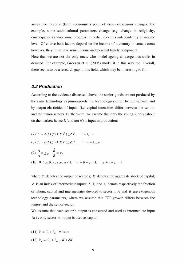
2.2 Production
According to the evidence discussed above, the senior-goods are not produced by
the same technology as junior-goods; the technologies differ by TFP-growth and
by output-elasticities of inputs (i.e. capital intensities differ between the senior-
and the junior-sector). Furthermore, we assume that only the young supply labour
on the market; hence L (and not N) is input in production:
(7) miZzKkLlAY iiii ,...1,)()()( == γβα
(8) nmiZzKkLlBY iiii ,...1,)()()( +== μνχ
(9) BA gB
Bg
A
A==
&&,
(10) 1;1;1,,,,,0 =++=++<< μνχγβαμνχγβα
where iY denotes the output of sector i; K denotes the aggregate stock of capital;
Z is an index of intermediate inputs; ii kl , and iz denote respectively the fraction
of labour, capital and intermediates devoted to sector i; A and B are exogenous
technology parameters, where we assume that TFP-growth differs between the
junior- and the senior-sector.
We assume that each sector’s output is consumed and used as intermediate input
)( ih ; only sector-m-output is used as capital:
(11) mihCY iii ≠∀+= ,
(12) KKhCY mmm δ+++= &
10
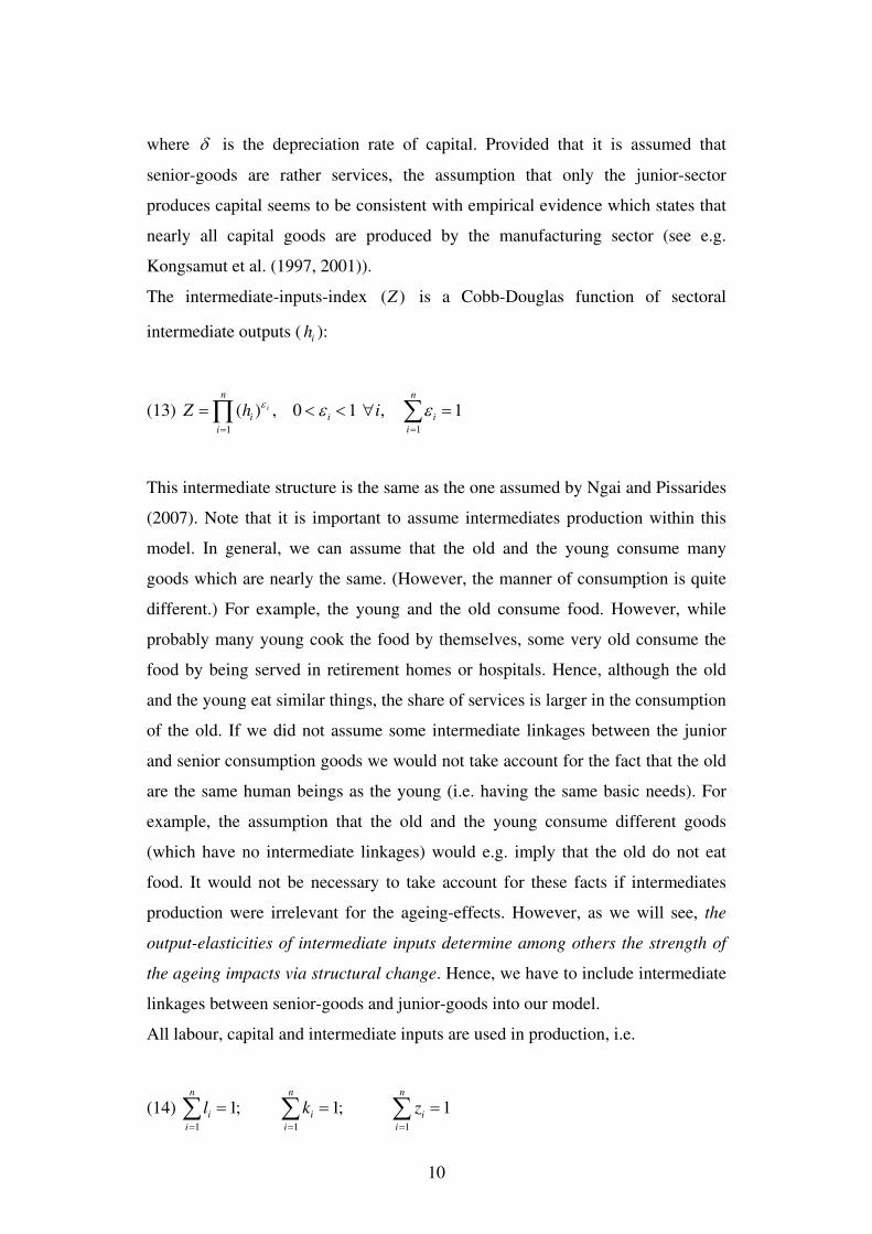
where δ is the depreciation rate of capital. Provided that it is assumed that
senior-goods are rather services, the assumption that only the junior-sector
produces capital seems to be consistent with empirical evidence which states that
nearly all capital goods are produced by the manufacturing sector (see e.g.
Kongsamut et al. (1997, 2001)).
The intermediate-inputs-index )(Z is a Cobb-Douglas function of sectoral
intermediate outputs ( ih ):
(13) ∑∏==
=∀<<=n
i
ii
n
i
i ihZ i
11
1,10,)( εεε
This intermediate structure is the same as the one assumed by Ngai and Pissarides
(2007). Note that it is important to assume intermediates production within this
model. In general, we can assume that the old and the young consume many
goods which are nearly the same. (However, the manner of consumption is quite
different.) For example, the young and the old consume food. However, while
probably many young cook the food by themselves, some very old consume the
food by being served in retirement homes or hospitals. Hence, although the old
and the young eat similar things, the share of services is larger in the consumption
of the old. If we did not assume some intermediate linkages between the junior
and senior consumption goods we would not take account for the fact that the old
are the same human beings as the young (i.e. having the same basic needs). For
example, the assumption that the old and the young consume different goods
(which have no intermediate linkages) would e.g. imply that the old do not eat
food. It would not be necessary to take account for these facts if intermediates
production were irrelevant for the ageing-effects. However, as we will see, the
output-elasticities of intermediate inputs determine among others the strength of
the ageing impacts via structural change. Hence, we have to include intermediate
linkages between senior-goods and junior-goods into our model.
All labour, capital and intermediate inputs are used in production, i.e.
(14) ∑∑∑===
===n
i
i
n
i
i
n
i
i zkl111
1;1;1
11
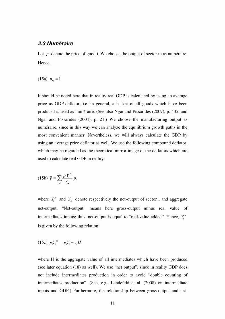
2.3 Numéraire
Let ip denote the price of good i. We choose the output of sector m as numéraire.
Hence,
(15a) 1=mp
It should be noted here that in reality real GDP is calculated by using an average
price as GDP-deflator; i.e. in general, a basket of all goods which have been
produced is used as numéraire. (See also Ngai and Pissarides (2007), p. 435, and
Ngai and Pissarides (2004), p. 21.) We choose the manufacturing output as
numéraire, since in this way we can analyze the equilibrium growth paths in the
most convenient manner. Nevertheless, we will always calculate the GDP by
using an average price deflator as well. We use the following compound deflator,
which may be regarded as the theoretical mirror image of the deflators which are
used to calculate real GDP in reality:
(15b) ∑=
≡n
i
i
N
N
ii pY
Ypp
1
where N
iY and NY denote respectively the net-output of sector i and aggregate
net-output. “Net-output” means here gross-output minus real value of
intermediates inputs; thus, net-output is equal to “real-value added”. Hence, N
iY
is given by the following relation:
(15c) HzYpYp iii
N
ii −=
where H is the aggregate value of all intermediates which have been produced
(see later equation (18) as well). We use “net output”, since in reality GDP does
not include intermediates production in order to avoid “double counting of
intermediates production”. (See, e.g., Landefeld et al. (2008) on intermediate
inputs and GDP.) Furthermore, the relationship between gross-output and net-
12
output in our model can be seen in equation (A.25) from APPENDIX A and
equations (16).)
Overall, our GDP-deflator (equation (15b)) is simply a weighted-average of
prices, where we used net-outputs as weights. If we divide our aggregate net-
output (expressed in manufacturing terms) by this deflator we have a GDP-
measure which is similar to the one which is used in reality. However, all the
issues regarding the choice of the numéraire are irrelevant when looking at
shares or ratios (since the changes in the numéraire of the numerator offset the
changes in the (same) numéraire of the denominator). For example, the capital-
to-output ratio ( NYK / ) is the same irrespective of the numéraire. (See also Ngai
and Pissarides (2007), p.435 and Ngai and Pissarides (2004), p.21.)
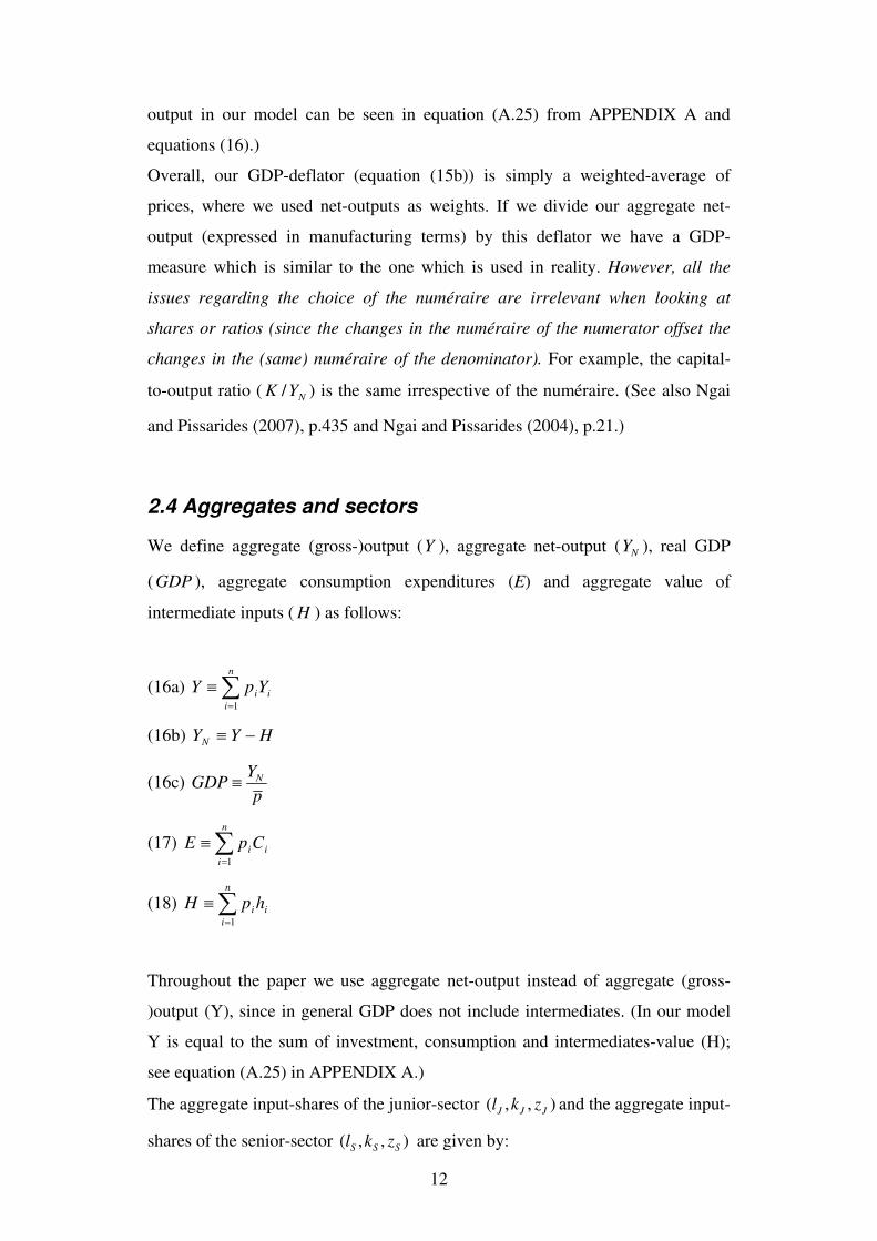
2.4 Aggregates and sectors
We define aggregate (gross-)output (Y ), aggregate net-output ( NY ), real GDP
(GDP ), aggregate consumption expenditures (E) and aggregate value of
intermediate inputs ( H ) as follows:
(16a) ∑=
≡n
i
iiYpY1
(16b) HYYN −≡
(16c) p
YGDP N≡
(17) ∑=
≡n
i
iiCpE1
(18) ∑=
≡n
i
iihpH1
Throughout the paper we use aggregate net-output instead of aggregate (gross-
)output (Y), since in general GDP does not include intermediates. (In our model
Y is equal to the sum of investment, consumption and intermediates-value (H);
see equation (A.25) in APPENDIX A.)
The aggregate input-shares of the junior-sector ),,( JJJ zkl and the aggregate input-
shares of the senior-sector ),,( SSS zkl are given by:
13
(19) ∑∑∑∑∑∑+=+=+====
≡≡≡≡≡≡n
mi
iS
n
mi
iS
n
mi
iS
m
i
iJ
m
i
iJ
m
i
iJ zzkkllzzkkll111111
,,,,,
The aggregate consumption expenditures on junior-goods ( JE ) and senior-goods
)( SE are given by:
(20) ∑∑+==
≡≡n
mi
iiS
m
i
iiJ CpECpE11
SE could also be interpreted as the budget devoted to the old. Throughout the
paper we assume that the aggregate budget is distributed across the old and the
young according to the representative household utility function (social welfare
function). That is, budgets are such to maximize social welfare.
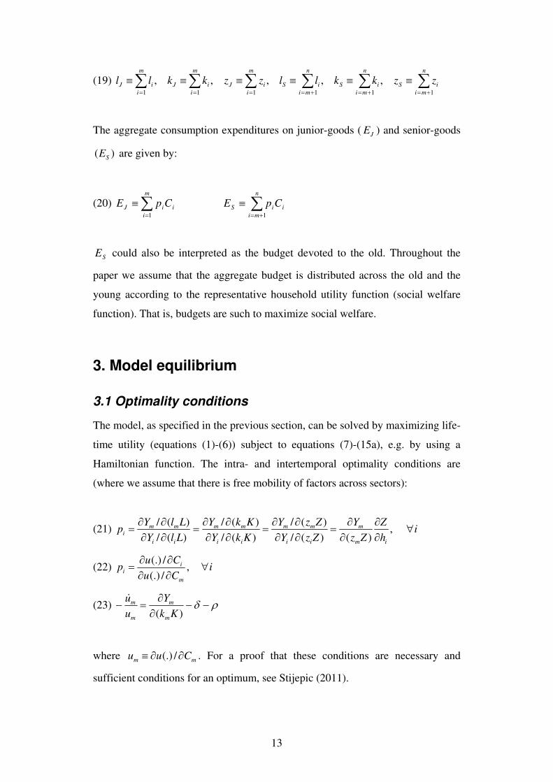
3. Model equilibrium
3.1 Optimality conditions
The model, as specified in the previous section, can be solved by maximizing life-
time utility (equations (1)-(6)) subject to equations (7)-(15a), e.g. by using a
Hamiltonian function. The intra- and intertemporal optimality conditions are
(where we assume that there is free mobility of factors across sectors):
(21) ih
Z
Zz
Y
ZzY
ZzY
KkY
KkY
LlY
LlYp
im
m
ii
mm
ii
mm
ii
mmi ∀
∂∂
∂∂
=∂∂∂∂
=∂∂∂∂
=∂∂∂∂
= ,)()(/
)(/
)(/
)(/
)(/
)(/
(22) iCu
Cup
m
ii ∀
∂∂∂∂
= ,/(.)
/(.)
(23) ρδ −−∂∂
=−)( Kk
Y
u
u
m
m
m
m&
where mm Cuu ∂∂≡ /(.) . For a proof that these conditions are necessary and
sufficient conditions for an optimum, see Stijepic (2011).
14
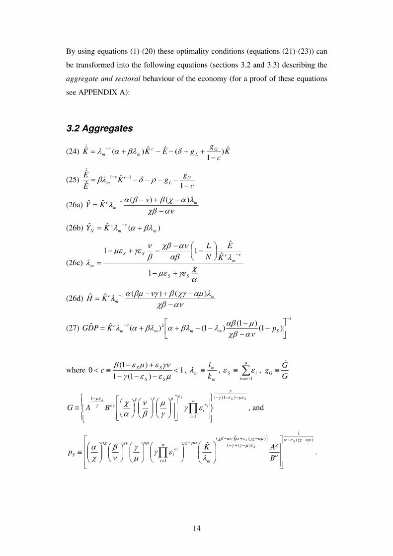
By using equations (1)-(20) these optimality conditions (equations (21)-(23)) can
be transformed into the following equations (sections 3.2 and 3.3) describing the
aggregate and sectoral behaviour of the economy (for a proof of these equations
see APPENDIX A):
3.2 Aggregates
(24) Kc
ggEKK G
L
c
m
c
mˆ)
1(ˆˆ)(ˆ
−++−−+= − δβλαλ&
(25) c
ggK
E
E GL
cc
m −−−−−= −−
1ˆ
ˆ
ˆ11 ρδβλ
&
(26a) ανχβ
λαχββαλ−
−+−= − mc
m
c vKY
)()(ˆˆ
(26b) )(ˆˆm
c
m
c
N KY βλαλ += −
(26c)
αχγεμε
λαβανχβ
βνγεμε
λSS
c
m
cSS
m
K
E
N
L
+−
⎟⎠⎞
⎜⎝⎛ −
−−+−
=−
1
ˆ
ˆ11
(26d) ανχβ
λαμχγβνγβμαλ−
−+−= − mc
m
cKH
)()(ˆˆ
(27)
1
2 )1()1(
)1()(ˆˆ−
−⎥⎦
⎤⎢⎣
⎡−
−−
−−++= Smmm
c
m
cpKPDG
ανχβμαβλβλαβλαλ
where 1)1(1
)1(0 <
−−−+−
≡<μεεγγνεμεβ
SS
SSc , m
m
mk
l≡λ , ∑
+=
≡n
mi
iS
1
εε , G
GgG
&≡
SS
i
S
S
S n
i
iBAG
μεεγγ
ε
εμνχεγ
με
εγγμ
βν
αχ
−−−
=
−
⎪⎭
⎪⎬⎫
⎪⎩
⎪⎨⎧
⎥⎥⎦
⎤
⎢⎢⎣
⎡⎟⎟⎠
⎞⎜⎜⎝
⎛⎟⎟⎠
⎞⎜⎜⎝
⎛⎟⎠⎞
⎜⎝⎛≡ ∏
)1(1
1
1
, and
[ ] )(
1
)(1
)()(
1
ˆαμγχεα
α
χεμγγαμγχεαανχβ
μαγχε
αμαναχ
λεγ
μγ
νβ
χα
−+−+−
−+−−
= ⎥⎥⎥
⎦
⎤
⎢⎢⎢
⎣
⎡
⎟⎟⎠
⎞⎜⎜⎝
⎛⎟⎟⎠
⎞⎜⎜⎝
⎛⎟⎟⎠
⎞⎜⎜⎝
⎛⎟⎠⎞
⎜⎝⎛
⎟⎟⎠
⎞⎜⎜⎝
⎛≡ ∏
S
S
S
i
B
AKp
m
n
i
iS .
15
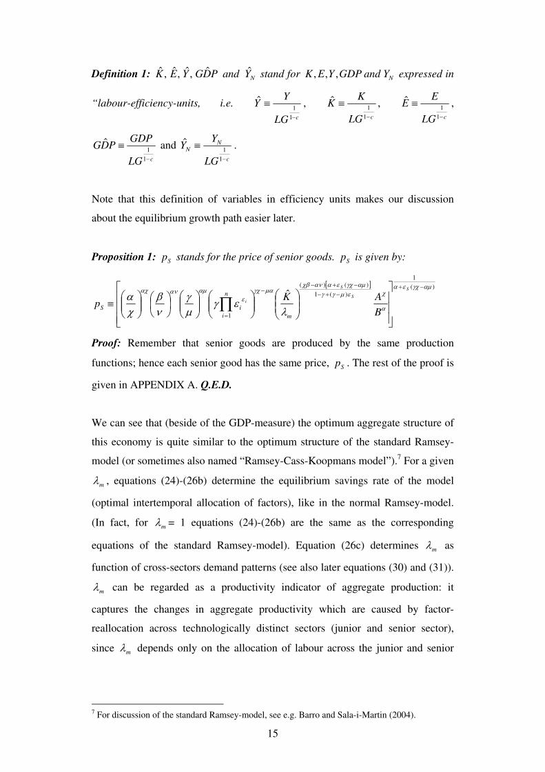
Definition 1: NYandPDGYEK ˆˆ,ˆ,ˆ,ˆ stand for NYandGDPYEK ,,, expressed in
“labour-efficiency-units, i.e.
cLG
YY
−
≡1
1ˆ ,
cLG
KK
−
≡1
1ˆ ,
cLG
EE
−
≡1
1ˆ ,
cLG
GDPPDG
−
≡1
1ˆ and
c
NN
LG
YY
−
≡1
1ˆ .
Note that this definition of variables in efficiency units makes our discussion
about the equilibrium growth path easier later.
Proposition 1: Sp stands for the price of senior goods. Sp is given by:
[ ] )(
1
)(1
)()(
1
ˆαμγχεα
α
χεμγγαμγχεαανχβ
μαγχε
αμαναχ
λεγ
μγ
νβ
χα
−+−+−
−+−−
= ⎥⎥⎥
⎦
⎤
⎢⎢⎢
⎣
⎡
⎟⎟⎠
⎞⎜⎜⎝
⎛⎟⎟⎠
⎞⎜⎜⎝
⎛⎟⎟⎠
⎞⎜⎜⎝
⎛⎟⎠⎞
⎜⎝⎛
⎟⎟⎠
⎞⎜⎜⎝
⎛≡ ∏
S
S
S
i
B
AKp
m
n
i
iS
Proof: Remember that senior goods are produced by the same production
functions; hence each senior good has the same price, Sp . The rest of the proof is
given in APPENDIX A. Q.E.D.
We can see that (beside of the GDP-measure) the optimum aggregate structure of
this economy is quite similar to the optimum structure of the standard Ramsey-
model (or sometimes also named “Ramsey-Cass-Koopmans model”).7 For a given
mλ , equations (24)-(26b) determine the equilibrium savings rate of the model
(optimal intertemporal allocation of factors), like in the normal Ramsey-model.
(In fact, for mλ = 1 equations (24)-(26b) are the same as the corresponding
equations of the standard Ramsey-model). Equation (26c) determines mλ as
function of cross-sectors demand patterns (see also later equations (30) and (31)).
mλ can be regarded as a productivity indicator of aggregate production: it
captures the changes in aggregate productivity which are caused by factor-
reallocation across technologically distinct sectors (junior and senior sector),
since mλ depends only on the allocation of labour across the junior and senior
7 For discussion of the standard Ramsey-model, see e.g. Barro and Sala-i-Martin (2004).
16
sectors: ⎟⎟⎠
⎞⎜⎜⎝
⎛+= SJm llβχανλ .
8 Furthermore, equation (26c) determines the mλ
which is consistent with the efficient (intratemporal) allocation of factors across
sectors, since equation (26c) can be derived from equations (14) and (21) (among
others); see as well the derivations in APPENDIX A. (Equations (14) state that all
factors must be used in production, i.e. no factors are wasted; equation (26c)
requires that marginal rates of technical substitution are equal across sectors, i.e.
factors are efficiently allocated across sectors.)
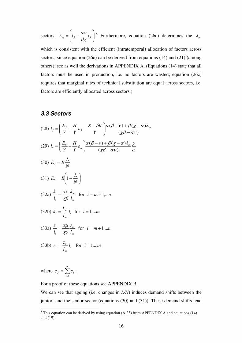
3.3 Sectors
(28) )(
)()(
ανχβλαχβνβαδε
−−+−
⎟⎟⎠
⎞⎜⎜⎝
⎛ +++= m
JJ
JY
KK
Y
H
Y
El
&
(29) αχ
ανχβλαχβνβαε
)(
)()(
−−+−
⎟⎠⎞
⎜⎝⎛ += m
SS
SY
H
Y
El
(30) N
LEEJ =
(31) ⎟⎠⎞
⎜⎝⎛ −=
N
LEES 1
(32a) m
m
i
i
l
k
l
k
χβαν
= for nmi ,...1+=
(32b) i
m
m
i ll
kk = for mi ,...1=
(33a) m
m
i
i
l
z
l
z
χγαμ
= for nmi ,...1+=
(33b) i
m
m
i ll
zz = for mi ,...1=
where ∑=
≡m
i
iJ
1
εε .
For a proof of these equations see APPENDIX B.
We can see that ageing (i.e. changes in L/N) induces demand shifts between the
junior- and the senior-sector (equations (30) and (31)). These demand shifts lead
8 This equation can be derived by using equation (A.23) from APPENDIX A and equations (14)
and (19).
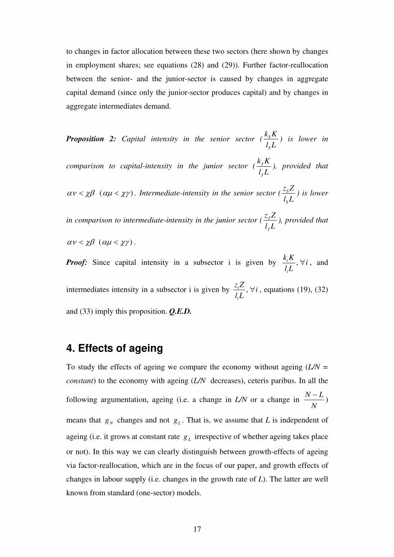
17
to changes in factor allocation between these two sectors (here shown by changes
in employment shares; see equations (28) and (29)). Further factor-reallocation
between the senior- and the junior-sector is caused by changes in aggregate
capital demand (since only the junior-sector produces capital) and by changes in
aggregate intermediates demand.
Proposition 2: Capital intensity in the senior sector (Ll
Kk
S
S ) is lower in
comparison to capital-intensity in the junior sector (Ll
Kk
J
J ), provided that
χβαν < ( )χγαμ < . Intermediate-intensity in the senior sector (Ll
Zz
S
S ) is lower
in comparison to intermediate-intensity in the junior sector (Ll
Zz
J
J ), provided that
χβαν < ( )χγαμ < .
Proof: Since capital intensity in a subsector i is given by iLl
Kk
i
i ∀, , and
intermediates intensity in a subsector i is given by iLl
Zz
i
i ∀, , equations (19), (32)
and (33) imply this proposition. Q.E.D.
4. Effects of ageing
To study the effects of ageing we compare the economy without ageing (L/N =
constant) to the economy with ageing (L/N decreases), ceteris paribus. In all the
following argumentation, ageing (i.e. a change in L/N or a change in N
LN −)
means that Ng changes and not Lg . That is, we assume that L is independent of
ageing (i.e. it grows at constant rate Lg irrespective of whether ageing takes place
or not). In this way we can clearly distinguish between growth-effects of ageing
via factor-reallocation, which are in the focus of our paper, and growth effects of
changes in labour supply (i.e. changes in the growth rate of L). The latter are well
known from standard (one-sector) models.
18
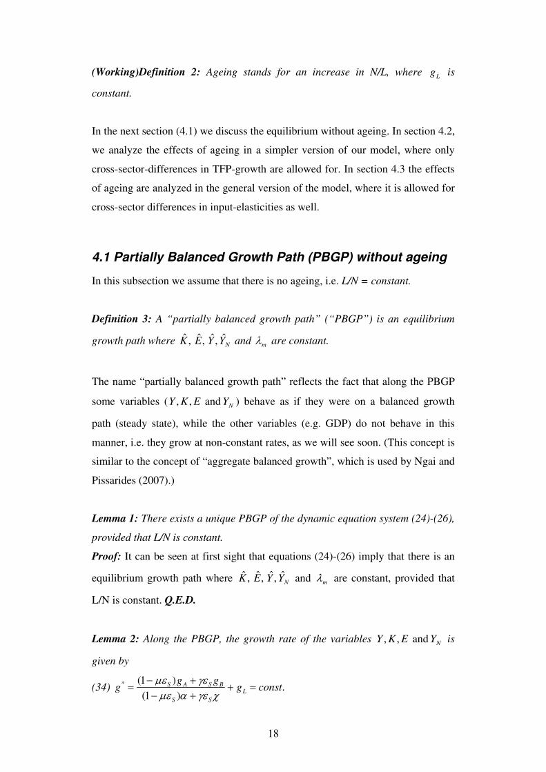
(Working)Definition 2: Ageing stands for an increase in N/L, where Lg is
constant.
In the next section (4.1) we discuss the equilibrium without ageing. In section 4.2,
we analyze the effects of ageing in a simpler version of our model, where only
cross-sector-differences in TFP-growth are allowed for. In section 4.3 the effects
of ageing are analyzed in the general version of the model, where it is allowed for
cross-sector differences in input-elasticities as well.
4.1 Partially Balanced Growth Path (PBGP) without ageing
In this subsection we assume that there is no ageing, i.e. L/N = constant.
Definition 3: A “partially balanced growth path” (“PBGP”) is an equilibrium
growth path where NYYEK ˆ ,ˆ,ˆ,ˆ and mλ are constant.
The name “partially balanced growth path” reflects the fact that along the PBGP
some variables ( NYEKY and ,, ) behave as if they were on a balanced growth
path (steady state), while the other variables (e.g. GDP) do not behave in this
manner, i.e. they grow at non-constant rates, as we will see soon. (This concept is
similar to the concept of “aggregate balanced growth”, which is used by Ngai and
Pissarides (2007).)
Lemma 1: There exists a unique PBGP of the dynamic equation system (24)-(26),
provided that L/N is constant.
Proof: It can be seen at first sight that equations (24)-(26) imply that there is an
equilibrium growth path where NYYEK ˆ ,ˆ,ˆ,ˆ and mλ are constant, provided that
L/N is constant. Q.E.D.
Lemma 2: Along the PBGP, the growth rate of the variables NYEKY and ,, is
given by
(34) .)1(
)1(* constggg
g L
SS
BSAS =++−+−
=χγεαμε
γεμε
19
(where L/N is constant).
Proof: This lemma is implied by Definitions 1 and 3. Q.E.D.
Lemma 3: Along the PBGP, factors are not shifted between the senior- and the
junior-sector, i.e. Jl and Sl are constant, (where L/N is constant).
Proof: This lemma is implied by equations (28)-(31), by Definitions 1 and 3 and
by Lemma 2. Q.E.D.
Definition 4: An asterisk (*) denotes the PBGP-value of the corresponding
variable.
Now, we derive the PBGP-values of variables as functions of exogenous
parameters:
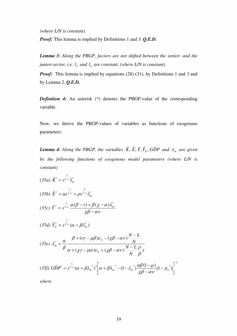
Lemma 4: Along the PBGP, the variables PDGYYEK Nˆ,ˆ ,ˆ,ˆ,ˆ and mλ are given
by the following functions of exogenous model parameters (where L/N is
constant)
(35a) *1
1
*ˆm
csK λ−=
(35b) *1
1
1*ˆm
cc
c
ssE λρα −− +=
(35c) ανχβ
λαχββα−
−+−= −
*
1* )()(ˆ mc
cv
sY
(35d) )(ˆ *1*
mc
c
N sY βλα += −
(35e)
sN
LNN
LN
S
S
m
βρανχβεμαχγα
ανχβεμβνγβ
βαλ
−−+−+
−−−−+
=)()(
)()(*
(35f)
1
***2*1* )1()1(
)1()(ˆ−
−⎥⎦
⎤⎢⎣
⎡−
−−
−−++= Smmmc
c
psPDGανχβμαβλβλαβλα
where
20
(35g)
[ ] )(
1
)(1
)()(
1
1
1
*
αμγχεα
α
χεμγγαμγχεαανχβ
μαγχε
αμαναχ
εγμγ
νβ
χα
−+−+−
−+−
−
−
= ⎥⎥⎥
⎦
⎤
⎢⎢⎢
⎣
⎡
⎟⎟⎠
⎞⎜⎜⎝
⎛⎟⎟⎠
⎞⎜⎜⎝
⎛⎟⎟⎠
⎞⎜⎜⎝
⎛⎟⎠⎞
⎜⎝⎛
⎟⎟⎠
⎞⎜⎜⎝
⎛= ∏
S
S
S
i
B
Asp c
n
i
iS
(35h)
c
gg
sG
L −+++
≡
1ρδ
β.
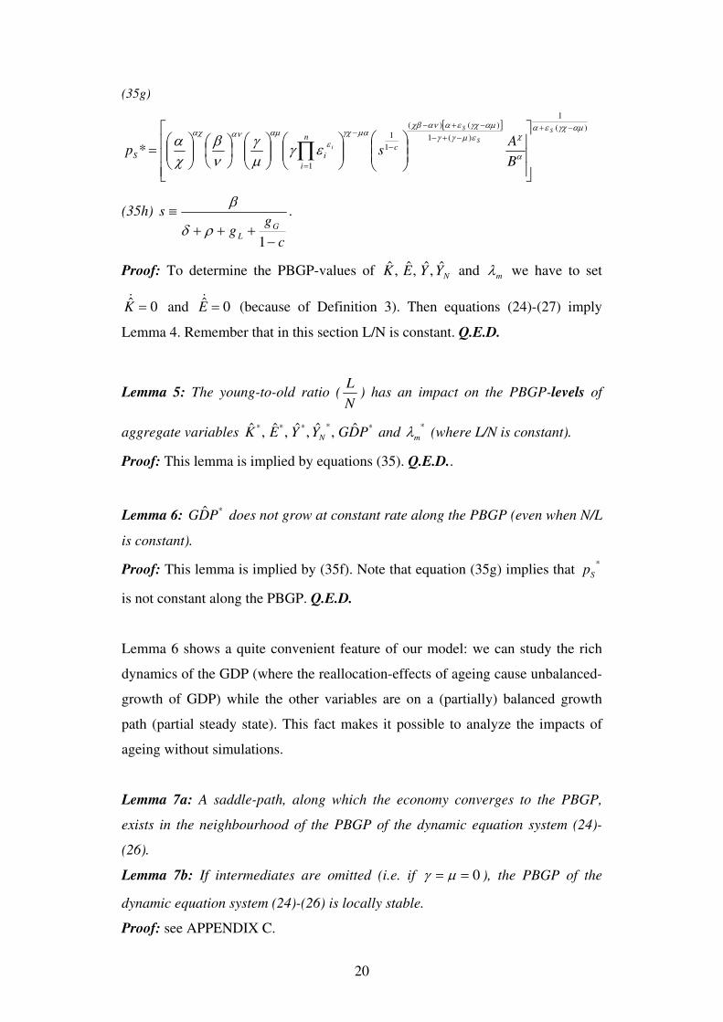
Proof: To determine the PBGP-values of NYYEK ˆ ,ˆ,ˆ,ˆ and mλ we have to set
0ˆ =K&
and 0ˆ =E&
(because of Definition 3). Then equations (24)-(27) imply
Lemma 4. Remember that in this section L/N is constant. Q.E.D.
Lemma 5: The young-to-old ratio (N
L) has an impact on the PBGP-levels of
aggregate variables ***** ˆ,ˆ ,ˆ,ˆ,ˆ PDGYYEK N and
*
mλ (where L/N is constant).
Proof: This lemma is implied by equations (35). Q.E.D..
Lemma 6: *ˆPDG does not grow at constant rate along the PBGP (even when N/L
is constant).
Proof: This lemma is implied by (35f). Note that equation (35g) implies that *
Sp
is not constant along the PBGP. Q.E.D.
Lemma 6 shows a quite convenient feature of our model: we can study the rich
dynamics of the GDP (where the reallocation-effects of ageing cause unbalanced-
growth of GDP) while the other variables are on a (partially) balanced growth
path (partial steady state). This fact makes it possible to analyze the impacts of
ageing without simulations.
Lemma 7a: A saddle-path, along which the economy converges to the PBGP,
exists in the neighbourhood of the PBGP of the dynamic equation system (24)-
(26).
Lemma 7b: If intermediates are omitted (i.e. if 0== μγ ), the PBGP of the
dynamic equation system (24)-(26) is locally stable.
Proof: see APPENDIX C.
21
Corollary 1: Even if the initial capital level is not given by equation (35a), the
economy which is described by the aggregate equation system (24)-(26)
converges to the PBGP, provided that L/N is constant.
Proof: This corollary follows from Lemmas 1, 4 and 7. Q.E.D.
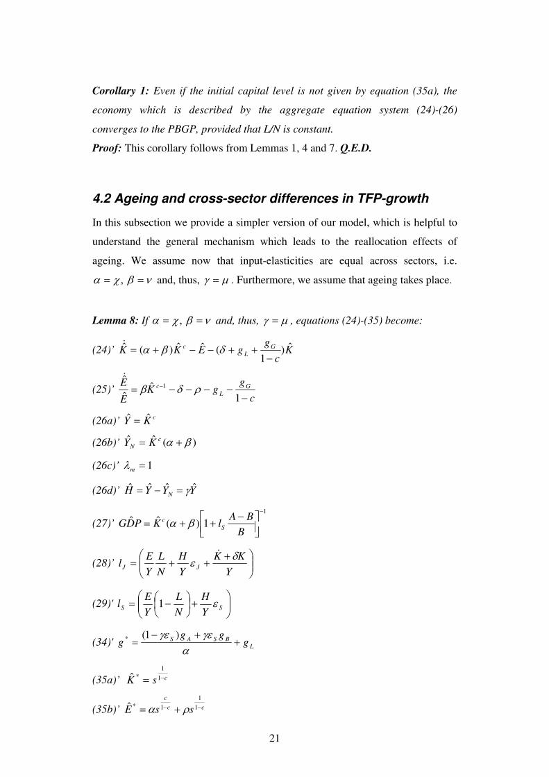
4.2 Ageing and cross-sector differences in TFP-growth
In this subsection we provide a simpler version of our model, which is helpful to
understand the general mechanism which leads to the reallocation effects of
ageing. We assume now that input-elasticities are equal across sectors, i.e.
νβχα == , and, thus, μγ = . Furthermore, we assume that ageing takes place.
Lemma 8: If νβχα == , and, thus, μγ = , equations (24)-(35) become:
(24)’ Kc
ggEKK G
L
c ˆ)1
(ˆˆ)(ˆ−
++−−+= δβα&
(25)’ c
ggK
E
E G
L
c
−−−−−= −
1ˆ
ˆ
ˆ1 ρδβ
&
(26a)’ c
KY ˆˆ =
(26b)’ )(ˆˆ βα += c
N KY
(26c)’ 1=mλ
(26d)’ YYYH Nˆˆˆˆ γ=−=
(27)’
1
1)(ˆˆ−
⎥⎦⎤
⎢⎣⎡ −++=
B
BAlKPDG S
c βα
(28)’ ⎟⎟⎠
⎞⎜⎜⎝
⎛ +++=
Y
KK
Y
H
N
L
Y
El JJ
δε&
(29)' ⎟⎟⎠
⎞⎜⎜⎝
⎛+⎟
⎠⎞
⎜⎝⎛ −= SS
Y
H
N
L
Y
El ε1
(34)' L
BSAS ggg
g ++−
=α
γεγε )1(*
(35a)’ csK −= 1
1
*ˆ
(35b)’ cc
c
ssE −− += 1
1
1*ˆ ρα
22
(35c)’ c
c
sY −= 1*ˆ
(35d)' )(ˆ 1* βα += −c
c
N sY
(35f)'
1
1* 1)(1)(ˆ−
−
⎭⎬⎫
⎩⎨⎧
⎥⎦
⎤⎢⎣
⎡+⎟
⎠⎞
⎜⎝⎛ −+
−++= S
c
c
N
Ls
B
BAsPDG γεραβα
where 10 <+
=<βα
βc ,
βαβα
εε
βα εγ+−−
=
+
⎪⎭
⎪⎬⎫
⎪⎩
⎪⎨⎧
⎥⎦⎤
⎢⎣⎡≡ ∏
1
1
1 n
i
ii
S
A
BAG .
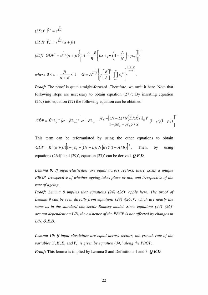
Proof: The proof is quite straight-forward. Therefore, we omit it here. Note that
following steps are necessary to obtain equation (27)’: By inserting equation
(26c) into equation (27) the following equation can be obtained:
[ ] 1
2 )1)(1(/1
)/ˆ/(ˆ/)()(ˆˆ
−
−⎥⎦
⎤⎢⎣
⎡−−
+−−−
−++= S
SS
c
mSmm
c
m
cp
KENLNKPDG μ
αχγεμελγεβλαβλαλ
This term can be reformulated by using the other equations to obtain
[ ][ ] 1
)/1(ˆ/ˆ/)(1)(ˆˆ−
−−+−+= BAYENLNKPDG S
c γεβα . Then, by using
equations (26d)’ and (29)’, equation (27)’ can be derived. Q.E.D.
Lemma 9: If input-elasticities are equal across sectors, there exists a unique
PBGP, irrespective of whether ageing takes place or not, and irrespective of the
rate of ageing.
Proof: Lemma 8 implies that equations (24)’-(26)’ apply here. The proof of
Lemma 9 can be seen directly from equations (24)’-(26c)’, which are nearly the
same as in the standard one-sector Ramsey model. Since equations (24)’-(26)’
are not dependent on L/N, the existence of the PBGP is not affected by changes in
L/N. Q.E.D.
Lemma 10: If input-elasticities are equal across sectors, the growth rate of the
variables NYEKY and ,,, is given by equation (34)’ along the PBGP.
Proof: This lemma is implied by Lemma 8 and Definitions 1 and 3. Q.E.D.

23
Lemma 11: If input elasticities are equal across sectors, the PBGP is globally
saddle-path stable, irrespective of whether ageing takes place or not.
Proof: Lemma 8 implies that equations (24)’-(26)’ apply. Equations (24)’ and
(25)’ are the same as in the standard Ramsey-model regarding all relevant
features. Therefore, the aggregate system of our model behaves like the standard
Ramsey-model, i.e. it is globally saddle-path stable. (See also Ngai and Pissarides
(2007) on the stability of such frameworks.). Since equations (24)’-(26)’ are
independent of L/N, ageing has no impact on the stability of the PBGP. Q.E.D.
Corollary 2: When input-elasticities are equal across sectors, ageing is irrelevant
regarding the development of the variables NYandEKY ,,, in our model: Neither
the PBGP-growth rate *
g nor the PBGP-levels **** ˆ andˆ,ˆ,ˆNYYEK are affected
by (the level or the growth rate of) L/N. A change in L/N does not induce a
deviation from the (initial) PBGP with respect to NYandEKY ,,, .
Proof: This corollary is implied by Lemmas 8-10 and equations (35). Q.E.D.
Now we take a look at the disaggregated variables of the economy.
Theorem 1: If input-elasticities are equal across sectors, ageing shifts demand
from the junior-sectors to the senior-sectors along the PBGP. That is, decreases
in L/N lead to decreases in EEJ / and increases in EES / .
Proof: This theorem is implied by equations (30) and (31). Remember that, as
argued in section 2, the choice of the numéraire is irrelevant when looking at
shares or ratios. Q.E.D.
Theorem 2: If input-elasticities are equal across sectors, ageing reallocates
factors from the junior-sectors to the senior-sectors along the PBGP; i.e.
decreases in L/N lead to decreases in Jl and increases in Sl .
Proof: This theorem is implied by Lemma 8 and equations (28)’ and (29)’.
Q.E.D.
Theorem 3: If input elasticities are equal across sectors, ageing reduces the
growth rate of GDP along the PBGP, provided that the TFP-growth rate (and the
24
TFP-level) is lower in the senior sector in comparison to the junior sector. That
is, a decreasing L/N causes a reduction of the GDP-growth rate, provided that
A>B and BA gg > .
Proof: This theorem is implied by Lemma 8 and equation (35f)’. Q.E.D.
Corollary 3: If input-elasticities are equal across sectors, ageing shifts demand
from the junior-sectors to the senior-sector. These demand shift cause factor
reallocation from the junior-sector to the senior-sector. This reallocation process
reduces the growth rate of GDP provided that the senior-sector has a relatively
low TFP(growth-rate) in comparison to the senior sector.
Proof: This corollary is implied by Theorems 1-3. Q.E.D.
Hence, whether ageing increases or decreases the GDP-growth-rate depends only
on the TFP-relation between the junior and senior sectors. The factors which
determine the strength of the ageing-impact are analyzed in the next section.
As argued in section 2, the choice of the numéraire is irrelevant when looking at
shares or ratios. Hence, we can analyze the senior-goods-consumption-to-output
ratio ( NS YE / ) without worrying about numéraire choice. The share of senior-
budget in aggregate output ( NS YE / ) increases at the same rate as the old-to-
young ratio (see equation (31) and remember that along the PBGP E and NY grow
at the same rate).
All the results from this section are valid for the case that the budget devoted to
seniors (e.g. old age pensions) develops according to the social welfare function
(representative household utility function). If however political issues led to a
reduction of old age pensions, the ageing-impacts would be weaker. We will
discuss this case later.
4.3 Ageing and cross-sector differences in input-
elasticities
Now let us assume that input-elasticities differ across sectors, i.e. νβχα ≠≠ ,
and μγ ≠ . (The TFP-growth rates differ across sectors as well.) Furthermore, in
25
this paper we analyze only the case where the capital intensity in the senior sector
is lower in comparison to the junior sector (i.e. χβαν < ), since this case is in
general assumed in the literature (see also Proposition 2). We assume that initially
the economy is in the equilibrium described in section 4.1 with L/N = constant. In
sections 4.3.1 and 4.3.2 we analyze what happens if there is a one time decrease
in L/N (according to Definition 2). (After this decrease L/N is constant again.) In
section 4.3.3 we generalize our results to the case where L/N increases
consecutively. Furthermore, in section 4.3.1 we analyze the effects of ageing on
net-output and on the pension-to-output ratio and we derive the impact channels,
whereas in section 4.3.2 we look at the differences in this analysis when our
GDP-measure is taken into account.
4.3.1 Productivity effect: Impacts and channels
In this subsection the term “aggregates” refers only to EYY N ,, and K but not to
GDP.
Lemma 12: A one time decrease in L/N leads to a change of the PBGP. That is,
the economy leaves the old PBGP and there is a transition period where the
economy converges to the new PBGP. The growth rate of aggregates (*
g ) is the
same along the old and the new PBGP.
Proof: Remember that we assume here again that the input-elasticities differ
across sectors; hence equations (24)-(35) apply here. Equations (35) imply that
there must be a transition period, since the old and the new PBGP require
different equilibrium capital levels; i.e. *K depends on L/N. (That is, the capital
level which exists when the decrease in L/N occurs is not the same as the capital
level which brings the economy directly on the new PBGP; we know from the
discussion of the standard one-sector Ramsey-model that this induces a transition
period, where the economy is converging to the new PBGP.) Furthermore,
Lemma 7 and Corollary 1 imply that the economy will converge to the new PBGP
(provided that the decrease in L/N is not too strong). Equation (34) implies that
the growth rate of aggregates ( *g ) is the same along the old and the new PBGP,
since *g does not depend on L/N. Q.E.D.
26
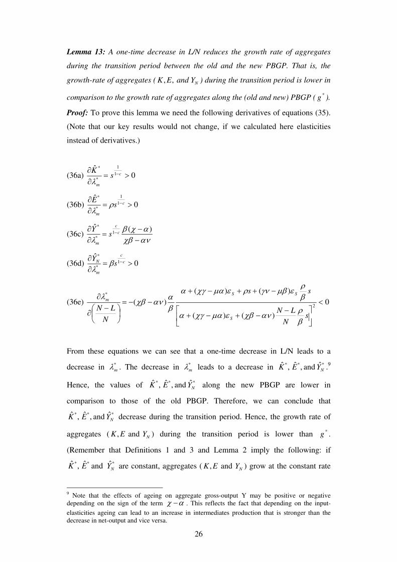
Lemma 13: A one-time decrease in L/N reduces the growth rate of aggregates
during the transition period between the old and the new PBGP. That is, the
growth-rate of aggregates ( NYandEK ,, ) during the transition period is lower in
comparison to the growth rate of aggregates along the (old and new) PBGP (*
g ).
Proof: To prove this lemma we need the following derivatives of equations (35).
(Note that our key results would not change, if we calculated here elasticities
instead of derivatives.)
(36a) 0ˆ
1
1
*
*
>=∂∂ −c
m
sK
λ
(36b) 0ˆ
1
1
*
*
>=∂∂ −c
m
sE ρλ
(36c) ανχβαχβ
λ −−
=∂∂ − )(ˆ
1*
*
c
c
m
sY
(36d) 0ˆ
1*
*
>=∂∂ −c
c
m
N sY βλ
(36e) 0
)()(
)()(
)(2
*
<
⎥⎦
⎤⎢⎣
⎡ −−+−+
−++−+−−=
⎟⎠⎞
⎜⎝⎛ −∂
∂
sN
LN
ss
N
LN
S
SS
m
βρανχβεμαχγα
βρεμβγνρεμαχγα
βαανχβ
λ
From these equations we can see that a one-time decrease in L/N leads to a
decrease in *
mλ . The decrease in *
mλ leads to a decrease in *** ˆ and ,ˆ,ˆNYEK .
9
Hence, the values of *** ˆ and ,ˆ,ˆNYEK along the new PBGP are lower in
comparison to those of the old PBGP. Therefore, we can conclude that
*** ˆ and ,ˆ,ˆNYEK decrease during the transition period. Hence, the growth rate of
aggregates ( NYEK and , ) during the transition period is lower than *g .
(Remember that Definitions 1 and 3 and Lemma 2 imply the following: if
*** ˆ and ˆ,ˆNYEK are constant, aggregates ( NYEK and , ) grow at the constant rate
9 Note that the effects of ageing on aggregate gross-output Y may be positive or negative
depending on the sign of the term αχ − . This reflects the fact that depending on the input-
elasticities ageing can lead to an increase in intermediates production that is stronger than the
decrease in net-output and vice versa.

27
*g ; hence, if
*** ˆ and ˆ,ˆNYEK decrease, the growth rate of NYEK and , is lower
than *g . Note that this argumentation works, since “efficiency units” are the same
along the old and the new PBGP: We express the variables in efficiency units (see
Definition 1) as follows: e.g. cLG
YY
−
≡1
1ˆ ; since cLG −1
1
does not change due to
ageing, efficiency units are the same along the old and the new PBGP.) Q.E.D.
We will discuss the intuition behind this lemma soon; at first we postulate two
lemmas, which are helpful to understand Lemma 13.
Lemma 14: A one-time decrease in L/N shifts demand from the junior-sector to
the senior-sector. That is, along the new PBGP E
ES is higher (E
EJ is lower) in
comparison to the E
ES (E
EJ ) of the old PBGP.
Proof: This lemma is implied by equations (30) and (31). Q.E.D.
Lemma 15: A one-time decrease in L/N leads to factor reallocation from the
junior-sector to the senior-sector. That is, along the new PBGP Sl is higher in
comparison to the Sl of the old PBGP.
Proof: By using equation (A.23) from APPENDIX A, it can be shown that the
employment share along the PBGP is given by ανχβ
χβλ−
−= )1(**
mSl . Since
equation (36e) implies that 0
1
*
<⎟⎠⎞
⎜⎝⎛ −∂
∂
N
Lmλ , a decrease in L/N leads to a decrease in
*
mλ . Therefore, *
Sl increases due to a decrease in L/N. (Remember that we
assume that 0>−ανχβ .) Q.E.D.
Now, we discuss the intuition behind Lemma 13: We know that output is
produced by using labour and capital. Ageing shifts demand (and, thus,
production factors) towards senior-sectors (as implied by Lemmas 14 and 15).
The key feature of the senior-sectors is that capital is less productivity-enhancing
28
in comparison to the (junior-sectors). This is reflected by the fact that optimal
capital intensity in the senior-sector is lower in comparison to the junior-sector
(see Proposition 2). Hence, the ageing-induced (one-time) demand-shift implies
that aggregate capital becomes less productive when looking at the economy-
wide-averages. Therefore, at the aggregate level a one-time decrease in L/N acts
similarly like a negative productivity-shock (a decrease in the productivity of
capital).10
This leads to the negative impacts on aggregate net-output-growth,
aggregate capital-growth and aggregate consumption-expenditures-growth (and of
course, the savings rate decreases, since savings which are invested in capital
become less rentable, i.e. the opportunity costs of consumption decrease). This
adjustment-process occurs during the transition period. Since a one-time
productivity-level-shock has no impacts on productivity-growth rates, the
economy converges to a growth path (PBGP) where the growth rate is the same as
before. (Remember that steady state growth rates are determined only by
productivity-growth and not by productivity-levels within the standard (one-
sector) Ramsey-model; in this respect our aggregate model is the same as the
standard Ramsey model.)
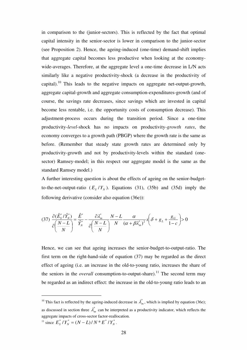
A further interesting question is about the effects of ageing on the senior-budget-
to-the-net-output-ratio ( NS YE / ). Equations (31), (35b) and (35d) imply the
following derivative (consider also equation (36e)):
(37) 01)(ˆ
ˆ)ˆ/ˆ(2*
*
*
***
>⎟⎠⎞
⎜⎝⎛
−++
+−
⎟⎠⎞
⎜⎝⎛ −∂
∂−=
⎟⎠⎞
⎜⎝⎛ −∂
∂c
ggs
N
LN
N
LNY
E
N
LN
YE GL
m
m
N
NS δβλααλ
Hence, we can see that ageing increases the senior-budget-to-output-ratio. The
first term on the right-hand-side of equation (37) may be regarded as the direct
effect of ageing (i.e. an increase in the old-to-young ratio, increases the share of
the seniors in the overall consumption-to-output-share).11
The second term may
be regarded as an indirect effect: the increase in the old-to-young ratio leads to an
10 This fact is reflected by the ageing-induced decrease in
*
mλ , which is implied by equation (36e);
as discussed in section three *
mλ can be interpreted as a productivity indicator, which reflects the
aggregate impacts of cross-sector factor-reallocation. 11 since
**** /*/)(/ NNS YENLNYE −= .
29
increase in the overall consumption-to-output-share12
(i.e. as noted above the
savings-rate decreases due to lower productivity level).
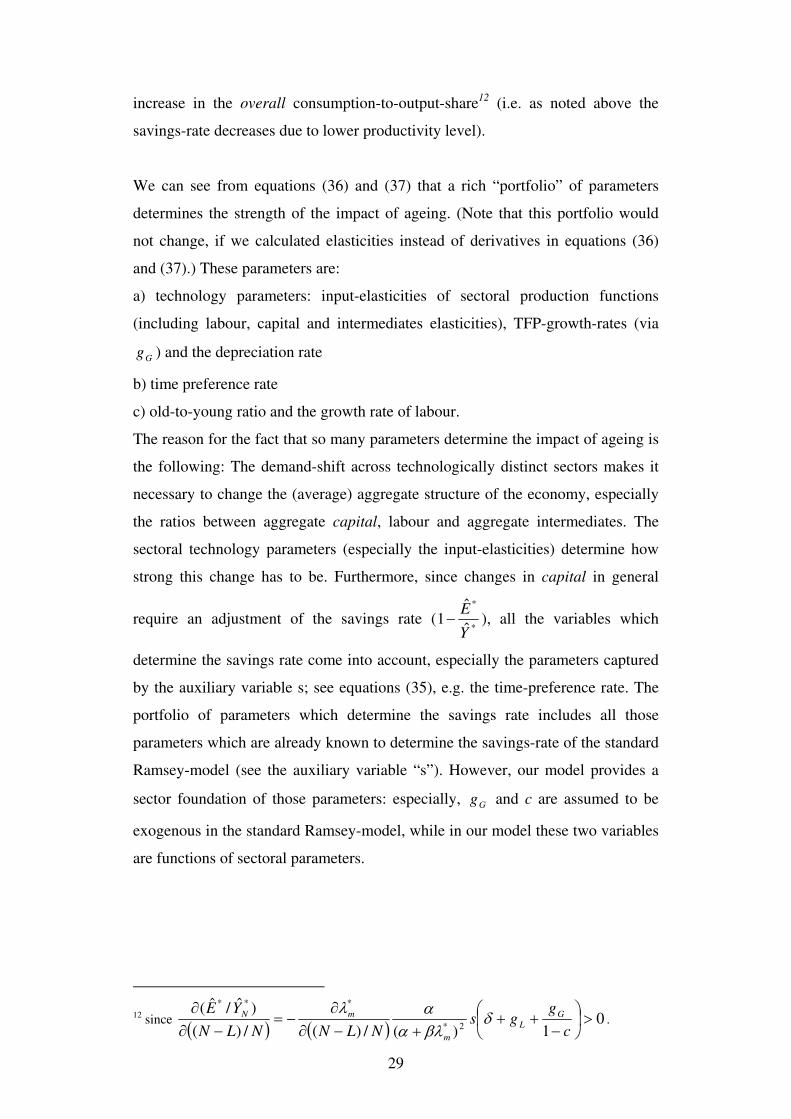
We can see from equations (36) and (37) that a rich “portfolio” of parameters
determines the strength of the impact of ageing. (Note that this portfolio would
not change, if we calculated elasticities instead of derivatives in equations (36)
and (37).) These parameters are:
a) technology parameters: input-elasticities of sectoral production functions
(including labour, capital and intermediates elasticities), TFP-growth-rates (via
Gg ) and the depreciation rate
b) time preference rate
c) old-to-young ratio and the growth rate of labour.
The reason for the fact that so many parameters determine the impact of ageing is
the following: The demand-shift across technologically distinct sectors makes it
necessary to change the (average) aggregate structure of the economy, especially
the ratios between aggregate capital, labour and aggregate intermediates. The
sectoral technology parameters (especially the input-elasticities) determine how
strong this change has to be. Furthermore, since changes in capital in general
require an adjustment of the savings rate (*
*
ˆ
ˆ1
Y
E− ), all the variables which
determine the savings rate come into account, especially the parameters captured
by the auxiliary variable s; see equations (35), e.g. the time-preference rate. The
portfolio of parameters which determine the savings rate includes all those
parameters which are already known to determine the savings-rate of the standard
Ramsey-model (see the auxiliary variable “s”). However, our model provides a
sector foundation of those parameters: especially, Gg and c are assumed to be
exogenous in the standard Ramsey-model, while in our model these two variables
are functions of sectoral parameters.
12 since ( ) ( ) 01)(/)(/)(
)ˆ/ˆ(2*
***
>⎟⎠⎞
⎜⎝⎛
−++
+−∂∂
−=−∂
∂c
ggs
NLNNLN
YE G
L
m
mN δβλααλ
.
30
4.3.2 Additional impacts on GDP: The price-effect
Remember that we have shown in the previous section that a one-time increase in
L/N leads to a transition from the old PBGP to a new PBGP. Due to this fact, the
effect of ageing on real GDP-growth can be divided into transitional effects and
PBGP-effects. Transitional effects have an impact on the real GDP-growth-rate
during the transition between two PBGPs, while PBGP-effects of ageing have an
impact on the growth rate along the new (PBGP). In fact we have shown that the
effects from the previous section are transitional. In this section we will introduce
a new effect which affects real GDP-growth (but not the growth rate of other
aggregate variables). We name this effect price effect, and we show that this
effect is not only transitional.
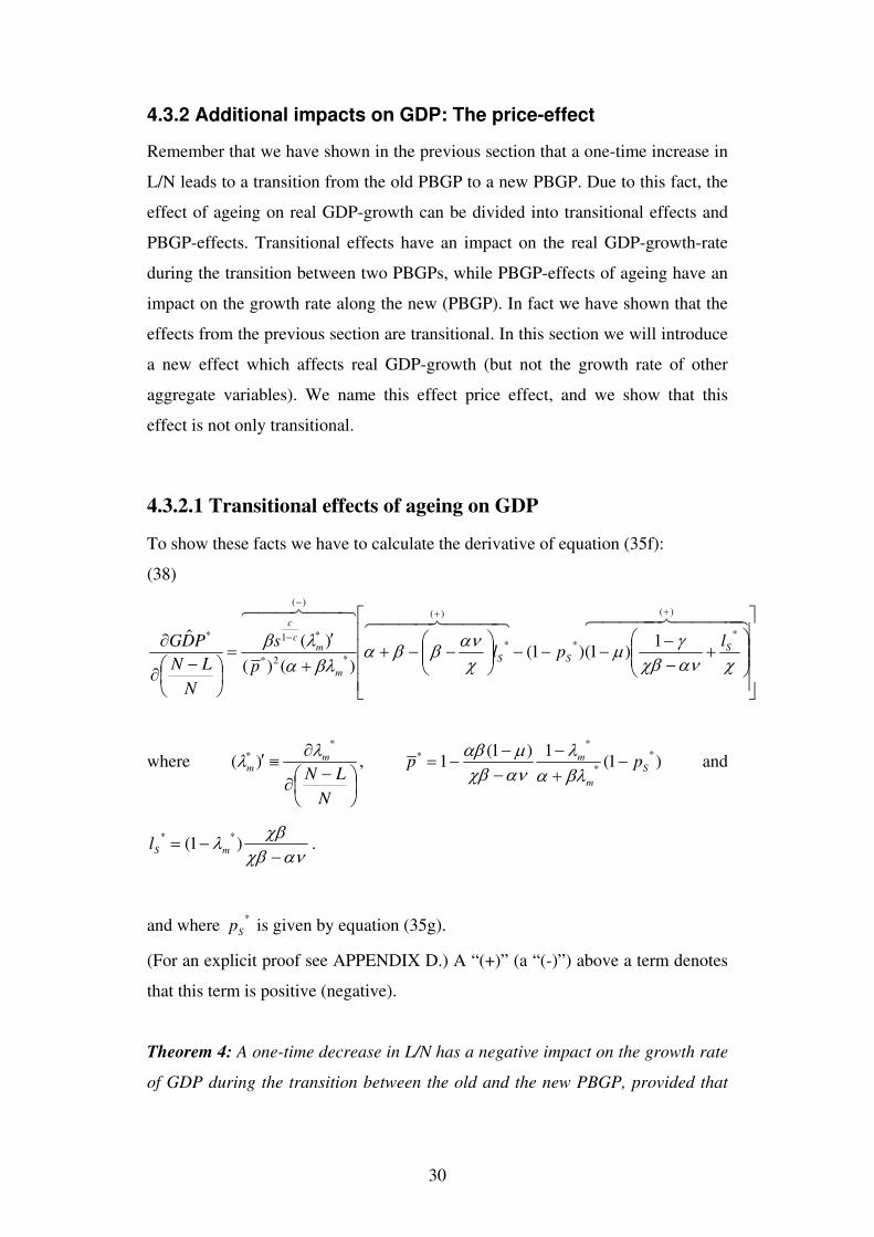
4.3.2.1 Transitional effects of ageing on GDP
To show these facts we have to calculate the derivative of equation (35f):
(38)
⎥⎥⎥⎥
⎦
⎤
⎢⎢⎢⎢
⎣
⎡
⎟⎟⎠
⎞⎜⎜⎝
⎛+
−−
−−−⎟⎟⎠
⎞⎜⎜⎝
⎛−−+
+′
=⎟⎠⎞
⎜⎝⎛ −∂
∂
++−
−
4444 84444 76444 8444 7644 844 76 )(
**
)(
*
)(
*2*
*1* 1)1()1(
)()(
)(ˆ
χανχβγμ
χανββα
βλαλβ S
SS
m
mc
c
lpl
p
s
N
LN
PDG
where
⎟⎠⎞
⎜⎝⎛ −∂
∂≡′
N
LNm
m
*
* )(λλ , )1(
1)1(1
*
*
*
*
S
m
m pp −+−
−−
−=βλαλ
ανχβμαβ
and
ανχβχβλ−
−= )1(**
mSl .
and where *
Sp is given by equation (35g).
(For an explicit proof see APPENDIX D.) A “(+)” (a “(-)”) above a term denotes
that this term is positive (negative).
Theorem 4: A one-time decrease in L/N has a negative impact on the growth rate
of GDP during the transition between the old and the new PBGP, provided that
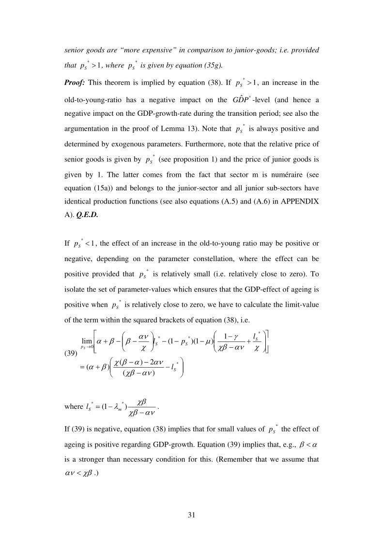
31
senior goods are “more expensive” in comparison to junior-goods; i.e. provided
that 1* >Sp , where
*
Sp is given by equation (35g).
Proof: This theorem is implied by equation (38). If 1* >Sp , an increase in the
old-to-young-ratio has a negative impact on the *ˆPDG -level (and hence a
negative impact on the GDP-growth-rate during the transition period; see also the
argumentation in the proof of Lemma 13). Note that *
Sp is always positive and
determined by exogenous parameters. Furthermore, note that the relative price of
senior goods is given by *
Sp (see proposition 1) and the price of junior goods is
given by 1. The latter comes from the fact that sector m is numéraire (see
equation (15a)) and belongs to the junior-sector and all junior sub-sectors have
identical production functions (see also equations (A.5) and (A.6) in APPENDIX
A). Q.E.D.
If 1* <Sp , the effect of an increase in the old-to-young ratio may be positive or
negative, depending on the parameter constellation, where the effect can be
positive provided that *
Sp is relatively small (i.e. relatively close to zero). To
isolate the set of parameter-values which ensures that the GDP-effect of ageing is
positive when *
Sp is relatively close to zero, we have to calculate the limit-value
of the term within the squared brackets of equation (38), i.e.
(39)
⎟⎟⎠
⎞⎜⎜⎝
⎛−
−−−
+=
⎥⎥⎦
⎤
⎢⎢⎣
⎡⎟⎟⎠
⎞⎜⎜⎝
⎛+
−−
−−−⎟⎟⎠
⎞⎜⎜⎝
⎛−−+
→
*
***
0
)(
2)()(
1)1)(1(lim
S
SSS
p
l
lpl
S
ανχβαναβχβα
χανχβγμ
χανββα
where ανχβ
χβλ−
−= )1(**
mSl .
If (39) is negative, equation (38) implies that for small values of *
Sp the effect of
ageing is positive regarding GDP-growth. Equation (39) implies that, e.g., αβ <
is a stronger than necessary condition for this. (Remember that we assume that
χβαν < .)
32
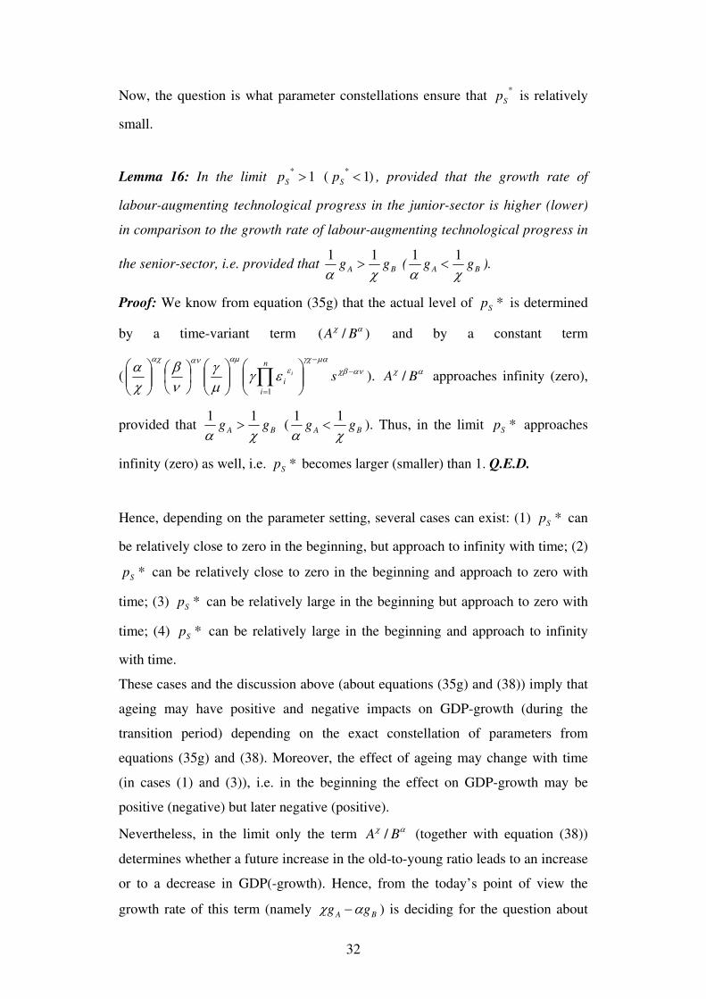
Now, the question is what parameter constellations ensure that *
Sp is relatively
small.
Lemma 16: In the limit 1* >Sp ( )1
* <Sp , provided that the growth rate of
labour-augmenting technological progress in the junior-sector is higher (lower)
in comparison to the growth rate of labour-augmenting technological progress in
the senior-sector, i.e. provided that BA ggχα11
> ( BA ggχα11
< ).
Proof: We know from equation (35g) that the actual level of *Sp is determined
by a time-variant term )/( αχBA and by a constant term
( ανχβμαγχ
εαμαναχ
εγμγ
νβ
χα −
−
=⎟⎟⎠
⎞⎜⎜⎝
⎛⎟⎟⎠
⎞⎜⎜⎝
⎛⎟⎠⎞
⎜⎝⎛
⎟⎟⎠
⎞⎜⎜⎝
⎛ ∏ sn
i
ii
1
). αχBA / approaches infinity (zero),
provided that BA ggχα11
> ( BA ggχα11
< ). Thus, in the limit *Sp approaches
infinity (zero) as well, i.e. *Sp becomes larger (smaller) than 1. Q.E.D.
Hence, depending on the parameter setting, several cases can exist: (1) *Sp can
be relatively close to zero in the beginning, but approach to infinity with time; (2)
*Sp can be relatively close to zero in the beginning and approach to zero with
time; (3) *Sp can be relatively large in the beginning but approach to zero with
time; (4) *Sp can be relatively large in the beginning and approach to infinity
with time.
These cases and the discussion above (about equations (35g) and (38)) imply that
ageing may have positive and negative impacts on GDP-growth (during the
transition period) depending on the exact constellation of parameters from
equations (35g) and (38). Moreover, the effect of ageing may change with time
(in cases (1) and (3)), i.e. in the beginning the effect on GDP-growth may be
positive (negative) but later negative (positive).
Nevertheless, in the limit only the term αχBA / (together with equation (38))
determines whether a future increase in the old-to-young ratio leads to an increase
or to a decrease in GDP(-growth). Hence, from the today’s point of view the
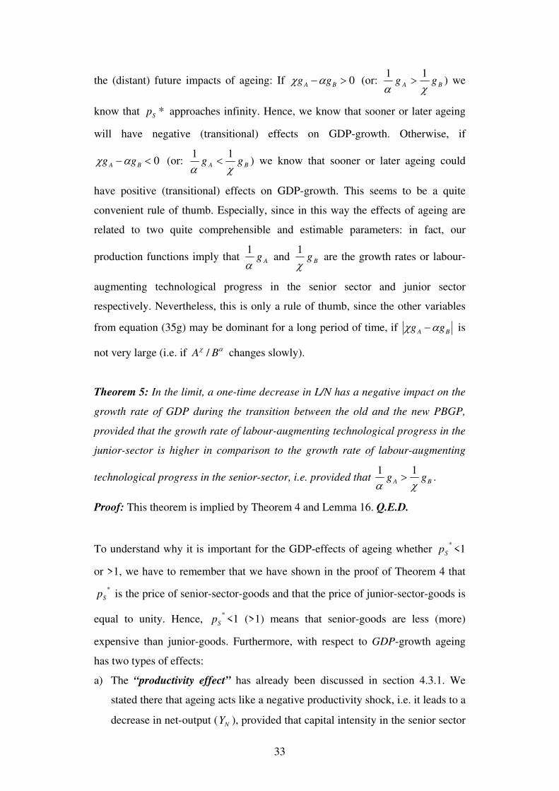
growth rate of this term (namely BA gg αχ − ) is deciding for the question about
33
the (distant) future impacts of ageing: If 0>− BA gg αχ (or: BA ggχα11
> ) we
know that *Sp approaches infinity. Hence, we know that sooner or later ageing
will have negative (transitional) effects on GDP-growth. Otherwise, if
0<− BA gg αχ (or: BA ggχα11
< ) we know that sooner or later ageing could
have positive (transitional) effects on GDP-growth. This seems to be a quite
convenient rule of thumb. Especially, since in this way the effects of ageing are
related to two quite comprehensible and estimable parameters: in fact, our
production functions imply that Agα1
and Bgχ1
are the growth rates or labour-
augmenting technological progress in the senior sector and junior sector
respectively. Nevertheless, this is only a rule of thumb, since the other variables
from equation (35g) may be dominant for a long period of time, if BA gg αχ − is
not very large (i.e. if αχBA / changes slowly).
Theorem 5: In the limit, a one-time decrease in L/N has a negative impact on the
growth rate of GDP during the transition between the old and the new PBGP,
provided that the growth rate of labour-augmenting technological progress in the
junior-sector is higher in comparison to the growth rate of labour-augmenting
technological progress in the senior-sector, i.e. provided that BA ggχα11
> .
Proof: This theorem is implied by Theorem 4 and Lemma 16. Q.E.D.
To understand why it is important for the GDP-effects of ageing whether *
Sp <1
or >1, we have to remember that we have shown in the proof of Theorem 4 that
*
Sp is the price of senior-sector-goods and that the price of junior-sector-goods is
equal to unity. Hence, *
Sp <1 (>1) means that senior-goods are less (more)
expensive than junior-goods. Furthermore, with respect to GDP-growth ageing
has two types of effects:
a) The “productivity effect” has already been discussed in section 4.3.1. We
stated there that ageing acts like a negative productivity shock, i.e. it leads to a
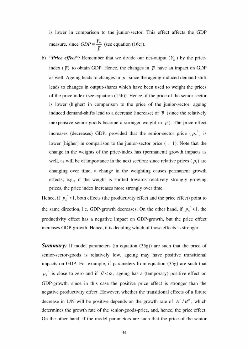
decrease in net-output ( NY ), provided that capital intensity in the senior sector
34
is lower in comparison to the junior-sector. This effect affects the GDP
measure, since p
YGDP N≡ (see equation (16c)).
b) “Price effect”: Remember that we divide our net-output ( NY ) by the price-
index ( )p to obtain GDP. Hence, the changes in p have an impact on GDP
as well. Ageing leads to changes in p , since the ageing-induced demand-shift
leads to changes in output-shares which have been used to weight the prices
of the price index (see equation (15b)). Hence, if the price of the senior sector
is lower (higher) in comparison to the price of the junior-sector, ageing
induced demand-shifts lead to a decrease (increase) of p (since the relatively
inexpensive senior-goods become a stronger weight in p ). The price effect
increases (decreases) GDP, provided that the senior-sector price (*
Sp ) is
lower (higher) in comparison to the junior-sector price ( = 1). Note that the
change in the weights of the price-index has (permanent) growth impacts as
well, as will be of importance in the next section: since relative prices ( ip ) are
changing over time, a change in the weighting causes permanent growth
effects; e.g., if the weight is shifted towards relatively strongly growing
prices, the price index increases more strongly over time.
Hence, if *
Sp >1, both effects (the productivity effect and the price effect) point to
the same direction, i.e. GDP-growth decreases. On the other hand, if *
Sp <1, the
productivity effect has a negative impact on GDP-growth, but the price effect
increases GDP-growth. Hence, it is deciding which of those effects is stronger.
Summary: If model parameters (in equation (35g)) are such that the price of
senior-sector-goods is relatively low, ageing may have positive transitional
impacts on GDP. For example, if parameters from equation (35g) are such that
*
Sp is close to zero and if αβ < , ageing has a (temporary) positive effect on
GDP-growth, since in this case the positive price effect is stronger than the
negative productivity effect. However, whether the transitional effects of a future
decrease in L/N will be positive depends on the growth rate of αχBA / , which
determines the growth rate of the senior-goods-price, and, hence, the price effect.
On the other hand, if the model parameters are such that the price of the senior
35
sector (*
Sp ) is higher than the price of the junior sector ( =1), ageing has a
negative transitional impact on GDP-growth, since the productivity effect and the
price effect point to the same direction. Whether future ageing will have negative
(transitional) effects in this case depends on the development of the term αχBA /
(and on the parameters of equation (35g)). Equations (35g) and (38) imply that
the parameter-portfolio which determines the strength and direction of the ageing-
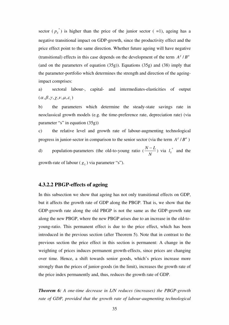
impact comprises:
a) sectoral labour-, capital- and intermediates-elasticities of output
( iεμνχγβα ,,,,,, )
b) the parameters which determine the steady-state savings rate in
neoclassical growth models (e.g. the time-preference rate, depreciation rate) (via
parameter “s” in equation (35g))
c) the relative level and growth rate of labour-augmenting technological
progress in junior-sector in comparison to the senior sector (via the term αχBA / )
d) population-parameters (the old-to-young ratio (N
LN −) via
*
Sl and the
growth-rate of labour ( Lg ) via parameter “s”).
4.3.2.2 PBGP-effects of ageing
In this subsection we show that ageing has not only transitional effects on GDP,
but it affects the growth rate of GDP along the PBGP. That is, we show that the
GDP-growth rate along the old PBGP is not the same as the GDP-growth rate
along the new PBGP, where the new PBGP arises due to an increase in the old-to-
young-ratio. This permanent effect is due to the price effect, which has been
introduced in the previous section (after Theorem 5). Note that in contrast to the
previous section the price effect in this section is permanent: A change in the
weighting of prices induces permanent growth-effects, since prices are changing
over time. Hence, a shift towards senior goods, which’s prices increase more
strongly than the prices of junior-goods (in the limit), increases the growth rate of
the price index permanently and, thus, reduces the growth rate of GDP.
Theorem 6: A one-time decrease in L/N reduces (increases) the PBGP-growth
rate of GDP, provided that the growth rate of labour-augmenting technological
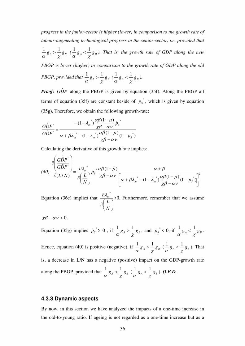
36
progress in the junior-sector is higher (lower) in comparison to the growth rate of
labour-augmenting technological progress in the senior-sector, i.e. provided that
BA ggχα11
> ( BA ggχα11
< ). That is, the growth rate of GDP along the new
PBGP is lower (higher) in comparison to the growth rate of GDP along the old
PBGP, provided that BA ggχα11
> ( BA ggχα11
< ).
Proof: PDG ˆ along the PBGP is given by equation (35f). Along the PBGP all
terms of equation (35f) are constant beside of *
Sp , which is given by equation
(35g). Therefore, we obtain the following growth-rate:
)1()1(
)1(
)1()1(
ˆ
ˆ
***
**
*
*
Smm
Sm
p
p
PDG
PDG
−−−
−−+
−−
−−=
ανχβμαβλβλα
ανχβμαβλ &&
Calculating the derivative of this growth rate implies:
(40) 2
***
***
*
)1()1(
)1(
)1(
)/(
ˆ
ˆ
⎥⎦
⎤⎢⎣
⎡−
−−
−−+
+−−
⎟⎠⎞
⎜⎝⎛∂
∂=
∂
⎟⎟
⎠
⎞
⎜⎜
⎝
⎛∂
Smm
Sm
p
p
N
LNL
PDG
PDG
ανχβμαβλβλα
βαανχβμαβλ
&
&
Equation (36e) implies that
⎟⎠⎞
⎜⎝⎛∂
∂
N
Lm
*λ>0. Furthermore, remember that we assume
0>−ανχβ .
Equation (35g) implies *
Sp& > 0 , if BA ggχα11
> , and *
Sp& < 0, if BA ggχα11
< .
Hence, equation (40) is positive (negative), if BA ggχα11
> ( BA ggχα11
< ). That
is, a decrease in L/N has a negative (positive) impact on the GDP-growth rate
along the PBGP, provided that BA ggχα11
> ( BA ggχα11
< ). Q.E.D.
4.3.3 Dynamic aspects
By now, in this section we have analyzed the impacts of a one-time increase in
the old-to-young ratio. If ageing is not regarded as a one-time increase but as a
37
sequence of (discrete) increases in the old-to-young ratio, our results still remain
applicable: Since we have shown in Lemma 7 (Corollary 1) that the PBGP is
saddle-path-stable, the economy will be on the converging path. The qualitative
results remain the same. The overall magnitude of the change in the macro-
variables (e.g. in GDP) is determined by the sum of the changes in the old-to-
young-ratio (overall-change in the old-to-young ratio). Only the period of change
(the transition period) is more prolonged, since the overall-change is dispersed
over a sequence (i.e. the economy cannot reach the “final” PBGP before the
sequence is finished).
5. Concluding remarks
In this paper we have specified how ageing affects the GDP-growth rate and the
pension-to-GDP-ratio via factor-allocation-effects. In the following we
summarize our results, compare them to previous literature, derive simple policy-
rules and predictions, show the caveats and extensions of our model and discuss
topics for further research.
5.1 The most important impact channels associated with factor-allocation-
effects
In our model ageing has three effects regarding GDP-growth:
(1) Direct productivity effect (structural change): The ageing-induced demand-
shift alters the factor allocation across technologically distinct sectors, which
yields a direct productivity effect (average factor-productivities change).
(2) Indirect productivity effect (capital accumulation): The “direct productivity
effect” has also an impact on GDP-growth via capital accumulation (change in the
savings rate). This effect is similar to the effect of a productivity(growth)-increase
in the standard one-sector Ramsey-model: a change in productivity leads to a
change in the opportunity costs of consumption, since return on savings depends
on productivity of capital (remember that savings are invested in capital). Note
that the change in the savings rate in our model is not the same as the ageing-
induced “savings-effect” in other ageing-models (e.g. in the models by Groezen et
al. (2005) and Rausch (2006)). In the latter models the effect of ageing on the

38
savings rate is modeled as a direct effect (“more saving for retirement, since we
live longer”).
(3) Price effect: Since the ageing-induced demand-shift leads to changes of
sectoral output-shares, the average price-index, which is the weighted average of
sector prices, changes as well. Hence, ageing leads to changes in GDP-deflator
(average price index), which has an impact on (real-)GDP as well.
5.2 Parameters which determine the strength and direction of the effects
We show that the strength and the direction of the factor-allocation-effects of
ageing depend on the combination of several parameters, including (see also the
Summary in section 4.3.2.1):
• technology parameters, e.g. sectoral TFP-growth-rates and (initial) TFP-levels
as well as input-elasticities of sectoral production functions (including
intermediates-elasticities, which supports Fougère et al. (2007) and Kuhn
(2004)),
• parameters determining the savings rate (due to effect (2)), e.g. the time-
preference rate, and
• population parameters (the old-to-young-ratio and the growth rate of working-
population).
5.3 Three simple implications for policy making and trend prediction
As shown in section 4.3.2, despite of its “complexity” our model provides quite
easily interpretable results, which can be used in empirical research and policy
making:
(1) The present and past effects of ageing via structural change can be assessed
by analyzing the (market) prices of senior-goods and junior-goods. In fact, our
model implies that ageing has a negative impact on real GDP-growth via
structural change, if senior goods are “more expensive” than junior goods.
Otherwise, if senior goods are cheaper, the effects of ageing can be positive or
negative, depending on the exact constellation of model parameters which are
summarized in section 5.2.
(2) For discussion of future effects of ageing analysis of parameters which
determine the development of relative prices of senior and junior sector is
necessary. Only in this way we can asses whether it makes sense to assume that
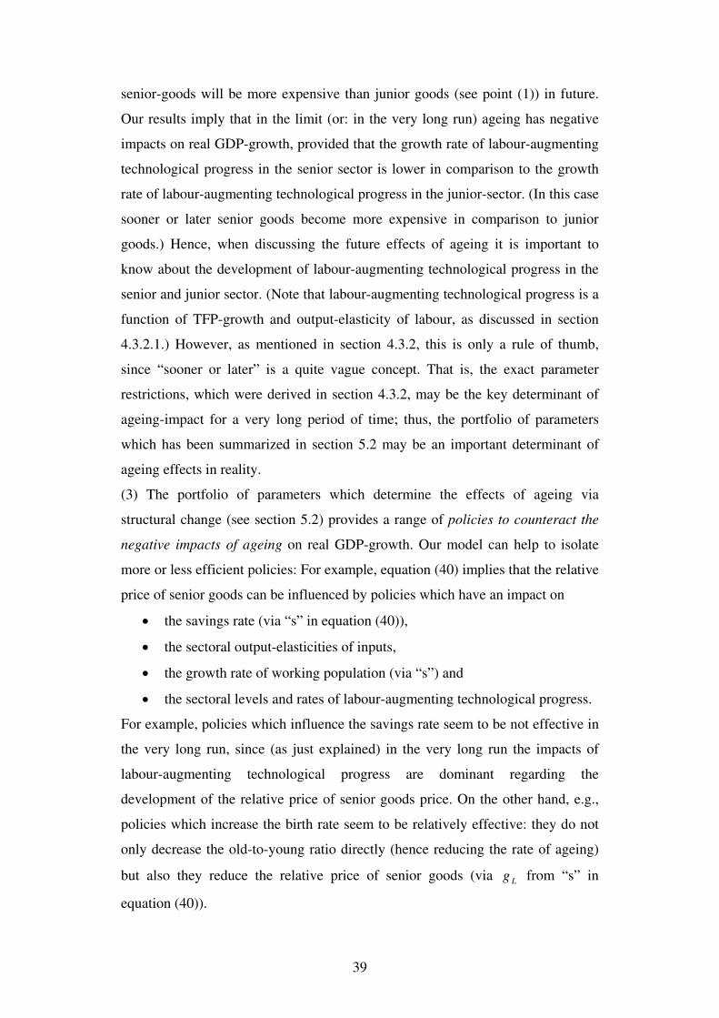
39
senior-goods will be more expensive than junior goods (see point (1)) in future.
Our results imply that in the limit (or: in the very long run) ageing has negative
impacts on real GDP-growth, provided that the growth rate of labour-augmenting
technological progress in the senior sector is lower in comparison to the growth
rate of labour-augmenting technological progress in the junior-sector. (In this case
sooner or later senior goods become more expensive in comparison to junior
goods.) Hence, when discussing the future effects of ageing it is important to
know about the development of labour-augmenting technological progress in the
senior and junior sector. (Note that labour-augmenting technological progress is a
function of TFP-growth and output-elasticity of labour, as discussed in section
4.3.2.1.) However, as mentioned in section 4.3.2, this is only a rule of thumb,
since “sooner or later” is a quite vague concept. That is, the exact parameter
restrictions, which were derived in section 4.3.2, may be the key determinant of
ageing-impact for a very long period of time; thus, the portfolio of parameters
which has been summarized in section 5.2 may be an important determinant of
ageing effects in reality.
(3) The portfolio of parameters which determine the effects of ageing via
structural change (see section 5.2) provides a range of policies to counteract the
negative impacts of ageing on real GDP-growth. Our model can help to isolate
more or less efficient policies: For example, equation (40) implies that the relative
price of senior goods can be influenced by policies which have an impact on
• the savings rate (via “s” in equation (40)),
• the sectoral output-elasticities of inputs,
• the growth rate of working population (via “s”) and
• the sectoral levels and rates of labour-augmenting technological progress.
For example, policies which influence the savings rate seem to be not effective in
the very long run, since (as just explained) in the very long run the impacts of
labour-augmenting technological progress are dominant regarding the
development of the relative price of senior goods price. On the other hand, e.g.,
policies which increase the birth rate seem to be relatively effective: they do not
only decrease the old-to-young ratio directly (hence reducing the rate of ageing)
but also they reduce the relative price of senior goods (via Lg from “s” in
equation (40)).
40
5.4 Further results and comparison to previous modelling-literature
It is unfair to compare our results to the results of previous modelling-literature,
since we have a different focus of analysis.13
Thus, the following discussion
should not be understood as critique of the previous literature; in our opinion, the
assumptions and model-choices which are made in previous literature are optimal
regarding the goals which are set there. Rather, we aim to emphasize those of our
results which are “new” in comparison to previous literature. Note that we omit
here the comparison of technical aspects of modelling and their impacts on the
results; furthermore, note that the discussion in sections 5.1 to 5.3 may be
regarded as “novelty” for the most part.
In contrast to Groezen et al. (2005), our model does not imply that low capital-
intensity in the senior sector is sufficient to constitute negative effects of ageing.
That is, lower capital-intensity in the senior sector does not necessarily imply that
senior goods are more expensive in comparison to junior goods. The reason is
that, in contrast to the model by Groezen et al. (2005), in our model the
“backward” sector is not completely stagnant, but features TFP-growth. Although
it is reasonable to assume that senior-goods are and will “always” be relatively
labour-intensive, it does not make sense to assume that they do not feature any
TFP-growth.14
Our model implies that such TFP-growth may offset the negative
impacts of high labour-intensity; thus negative impacts of ageing may not arise in
this case. Thus, the focus of analysis should be shifted to labour-augmenting
technological progress, which takes account of both (output-elasticity of capital
and TFP-growth); see also point (2) in section 5.3.
Anyway, as discussed in section 5.3 (points (2) and (3)), in most cases the
impacts of ageing in reality may not be determined by the analysis of only few of
such variables, but the exact parameter constellation of a relatively large
parameter portfolio (see section 5.2) may be deciding. Therefore, the strength and
direction of factor-allocation-effects of ageing may vary strongly across countries
13 Groezen et al. (2005)-focus is on trade-off between “savings effect” and “factor-allocation-
effect”, see section 1.3, while our focus is on detailed modeling of the “factor-allocation-effect”,
see section 1.4. 14 Let us take a very extreme example: The services of a psychologist seem to be very labour-
intensive. That is, it is very difficult to imagine today, that even in far future a machine will be
invented, which is able to substitute the human psychologist (or its ability to understand the
emotions of the patient). Thus, we may assume that labour-intensity in this profession
(psychologist) will always be very high. Nevertheless, it is reasonable to assume that psychology
(as a science) will make some progress, and, thus, the productivity of the psychologist will
increase, i.e. the TFP of psychological service provision will increase in future.
41
depending upon their values of these parameters. The fact that empirical studies
were not able to identify an unambiguous effect of ageing on growth (see
Groezen et al. (2005)) may come from the neglect of the importance of cross-
country differences in this parameter portfolio.
The following result is related to this discussion as well: In contrast to the
previous literature we show (in section 4.3.2) that the impacts of ageing on GDP-
growth may be non-monotonous over time, i.e. in the beginning ageing may have
a positive (negative) impact on GDP-growth and later the effect of ageing may be
negative (positive).15
This result, as well, implies that the strength of the ageing
impact (and the necessary reforms of pension systems) may vary widely across
countries and across time, depending on the parameters derived in our model.
Last not least, we introduced the “price effect” in our paper (see also section 5.1
point (3)). This effect is predominant in sections 4.2 and 4.3.2.2. In fact, it is the
only “persistent” effect of a one-time increase in the old-to-young-ratio. Thus, this
effect elucidates the theoretical importance of ageing for growth: even a one time-
increase in the old-to-young ratio is associated with a permanent change in the
(equilibrium) growth rate of real GDP.
Overall, our results imply that from the theoretical point of view factor-allocation-
effects of ageing have significant impacts on the long-run GDP-growth rate.
Projections of future GDP-growth and of future pension-system-challenges may
be too optimistic. For example, the paper by the Economic Policy Committee of
the EU Commission (2003) based on Mc Morrow and Röger (2003) (see there
especially pp. 12 ff.) does not include factor-allocation-effects in its ageing-
related projections. Hence, the negative impacts of ageing may be stronger than
expected by now and the reforms of old-age-pension systems (and health-
systems) may be too weak. Furthermore, theories which try to explain the
past/historic development of aggregates (e.g. Kaldor-facts) without accounting for
factor-allocation-effects of ageing seem to omit important determinants of
15 This non-monotonousity comes from the fact that, although the senior sector has relatively low
capital intensity, the price of senior-goods needs not necessarily being higher than the price of
junior-goods. That is, the positive “price effect” of ageing can overweight the negative
“productivity effects” of ageing. However, if the growth rate of labour-augmenting technological
progress is relatively high in the junior sectors, the senior goods must become more expensive
than junior goods at some point of time, i.e. the price effect becomes negative as well. (See also
the explanations at the beginning of section 5.4 (second paragraph)).
42
aggregate development. In general, ageing causes unbalanced growth of sectors
and aggregates in our model.
5.5 The usefulness of PBGPs
From a theoretical point of view our model demonstrates the usefulness of
partially balanced growth paths in dynamic analysis: In contrast to most literature,
which searches for balanced growth paths of variables of interest, we used a
different approach: Although we are interested in the development of GDP and
sectoral employment shares, we did not analyze the balanced growth paths of
these variables, since these growth paths are not interesting from a theoretical
point of view (because they do not allow for structural change). Instead, we
analyzed our variables of interest along the balanced growth path of an auxiliary
dynamic system, which consisted of variables Y, K and E. We named the
balanced growth path of this auxiliary system “PBGP”. In section 4.2 we
analyzed our variables of interest along the PBGP, while in section 4.3 we
analyzed the transitional dynamics between two PBGPs and compared the PBGP-
dynamics of two equilibriums. Overall, the usage of PBGPs helped us to
analytically study a topic which otherwise would require simulations.
5.6 A word on challenges to pension-systems
Needless to say that our paper has also implications for all the literature and
predictions which deal with the challenges to old-age-pension and health-systems
associated with ageing. If the ageing-induced change in GDP-growth is negative,
there is additional upward-pressure on the pension-to-output ratio. (Remember
that upward pressure on the pension-to-output-ratio comes from an increasing
number of pension-recipients as well).
5.7 Extension of our model: Endogenous technology
The existence and strength of “factor-allocation-effects” of ageing depends upon
the existence and strength of technology-bias. “Technology-bias” means here
cross-sector-difference in technology: we assume that senior-goods-sectors do not
use the same technology as junior-goods-sectors. If this bias vanished, i.e. if both
sectors had the same technology, the factor allocation across the two sectors
would be irrelevant regarding GDP-growth. Thus, there would not be any factor-
43
allocation-effect of ageing. In the introduction of the paper we provided literature-
references which imply that the technology-bias exists in reality. In our model the
technology(-bias) is exogenous; ageing has no impact on the technology-bias.
Stijepic and Wagner (2011) provide an extension of our model, where the
technology-bias is endogenized. They show that ageing-related demand-shifts can
have an impact on the technology-bias (see section 5 in that paper). Nevertheless,
their results do not imply that any of our results is incorrect. However, their
results imply that additional forces have an impact on the strength of the factor-
allocation-effects of ageing: in fact, all the forces which influence the technology-
bias (e.g. sort of implementation of technological progress, dispersion of capital
across sectors, etc) have also an impact on the factor-allocation-effects of ageing
discussed in this essay. Note, however, that all these forces determine the strength
of the factor-allocation-effects of ageing, but not the direction. An extensive
discussion of these forces is provided by Stijepic and Wagner (2011).
5.8 Caveats and topics for further research
Throughout the paper we assumed that parameter restrictions (5a,b) hold. In fact,
these restrictions ensure that there are no other sources of demand-shifts between
the senior and junior sector beside of ageing. However, the impact of social
welfare parameters (especially, the question how the utility of the old and the
young is weighted in a society) may be captured by deviation from these
restrictions. The question is whether pension systems (and private “savings-for-
retirement”-behaviour) change systematically (i.e. whether the weight is shifted to
the old or to the young) with an increasing income. The answer to this question
decides whether the budget-share of the old increases/decreases over the growth
process. The higher the budget for senior-goods consumption (per old person), the
stronger the factor-allocation-effects of ageing. Income-dependent changes in
pension-systems could be modelled by a departure from the restrictions (5a,b).
Furthermore, it should be mentioned here that, if the budget of the old ( SE ) was
restricted by an exogenous force (e.g. by an “inefficient” pension system) in our
model, the ageing impacts on GDP-growth would be weaker. However, from the
social welfare point of view this would be suboptimal (i.e. the social welfare
would be suboptimal).
44
These facts may as well have some explanatory power regarding differences in
the strength of ageing impacts across countries.
In section 4.3 we modelled ageing like a shock (or series of shocks) and not like a
smooth and perfectly foresighted process. The difference between these two
approaches is that the latter is more difficult to model (We could not rely on the
PBGP-results) and we would have to use simulations. Furthermore, if perfectly
foresighted the effects of ageing would be smoother, i.e. dispersed over a longer
period (i.e. even before the increase in the old-to-young ratio the effects of ageing
would show up), which would affect our results quantitatively but not
qualitatively (i.e. the impact channels would be the same). Furthermore, it should
be questioned whether it makes sense to model ageing like a smooth perfectly
foresighted process, especially when taking into account irrational or bounded
rational behaviour of households in reality. Last but not least, since our model is
aimed to postulate some crude qualitative relationships between macroeconomic
parameters and variables, the question whether ageing is modelled as a series of
shocks or as a perfectly foresighted smooth process seems to be less relevant.
Overall, our results imply that for assessing (the future) growth-impacts of ageing
some further empirical research is necessary to estimate the exact technological
properties of the junior and senior sector. Especially, it seems to be necessary to
link the data on demand-differences across the old and the young with the data on
technological properties of the sectors. Only in this way a general conclusion can
be drawn about the past and future strength of the ageing impacts. Furthermore,
the question whether the senior sector will have a lower growth rate of labour-
augmenting technological progress in future seems to be interesting regarding the
effects of ageing.
Last not least, as mentioned in Section 2.1, it could be interesting to endogenize
the population development (e.g. old-to-young ratio as a function of income) and
to analyze which factor-allocation-effects arise in such a model. However, the
results of such an exercise are approximated by standard structural change
literature, as discussed in Section 2.1.
Analyzing these questions is left for further research.
45
References
Acemoglu D (2009). Introduction to Modern Economic Growth. Princeton
University Press.
Acemoglu D, Guerrieri V (2008). Capital Deepening and Nonbalanced
Economic Growth. Journal of Political Economy, 116(3): 467-498.
Barro RJ, Sala-i-Martin X (2004). Economic Growth. 2nd edition. MIT Press.
Cambridge, Mass.
Baumol WJ (1967). Macroeconomics of Unbalanced Growth: The Anatomy of
Urban Crisis. American Economic Review, 57(3): 415-426.
Baumol WJ, Batey-Blackman SA, Wolf EN (1985). Unbalanced Growth
Revisited: Asymptotic Stagnancy and New Evidence. American Economic
Review, 57(3): 415-426.
Bernard AB, Jones CI (1996). Comparing Apples to Oranges: Productivity
Convergence and Measurement across Industries and Countries. American
Economic Review, 86(5): 1216-1238.
Berthélmy JC, Söderling L (1999). The Role of Capital Accumulation,
Adjustment and Structural Change for Economic Take-off: Empirical Evidence
from African Growth Episodes, OECD Development Centre Working Paper No.
150.
Börsch-Supan A (1993). Aging in Germany and the United States: International
Comparisons. NBER Working Paper 4530.
Börsch-Supan A (2003). Labor Market Effects of Population Aging. LABOR,
17(Special Issue): 5-44.
Broadberry SN (1997). The Long Run Growth and Productivity Performance of
the United Kingdom, Scottish Journal of Political Economy, 44(4): 403-424.
Broadberry SN (1998). How Did the United States and Germany Overtake
Britain? A Sectoral Analysis of Comparative Productivity Levels, 1870-1990”,
The Journal of Economic History, 58(2): 375-407.
Broadberry SN, Irwin DA (2006). Labor Productivity in the United States and
the United Kingdom during the Nineteenth Century, Explorations in Economic
History, 43: 257–279.
46
Caselli F, Coleman WJII (2001). The U.S. Structural Transformation and
Regional Convergence: A Reinterpretation, Journal of Political Economy, 109(3):
584-616.
Close FA, Shulenburger DE (1971). Labor’s Share by Sector and Industry,
1948-1965. Industrial and Labor Relations Review, 24(4): 588-602.
Disney R, Haskel J, Heden Y. (2003). Restructuring and Productivity Growth in
UK Manufacturing, The Economic Journal, 113: 666–694.
Dowrick S, Gemmel N (1991). Industrialisation, Catching up and Economic
Growth: A Comparative Study across the World’s Capitalist Economies, The
Economic Journal, 101: 263-275.
Duarte M, Restuccia D (2010). The Role of the Structural Transformation in
Aggregate Productivity, The Quarterly Journal of Economics, 125(1): 129-173.
Economic Policy Committee of the EU Commission (2003). The Impact of
Ageing Populations on Public Finances: Overview of Analysis Carried out at EU
Level and Proposals for a Future Work Programme. EPC/ECFIN/435/03 final.
Foster L, Haltiwanger J, Krizan CJ (1998). Aggregate Productivity Growth:
Lessons from Microeconomic Evidence, NBER Working Paper 6803.
Fougère M, Mercenier J, Mérette M (2007). A Sectoral and Occupational
Analysis of Population Ageing in Canada Using a Dynamic CGE Overlapping
Generations Model. Economic Modelling, 24(4): 690-711.
Fuchs VR (1998). Provide, Provide: The Economics of Aging. NBER Working
Paper 6642.
Gollin D (2002). Getting Income Shares Right. Journal of Political Economy,
110(2): 458-474.
Groezen van B, Meijdam L, Verbon HAA (2005). Serving the Old: Ageing and
Economic Growth. Oxford Economic Papers, 57(4): 647-663.
Gruescu S (2007). Population Ageing and Economic Growth. Physica.
Heidelberg.
International Monetary Fund (IMF) (2004). World Economic Outlook: The
Global Demographic Transition. Chapter III: How Will Demographic Change
Affect the Global Economy? Available on the web at:
http://www.imf.org/External/Pubs/FT/weo/2004/02/pdf/chapter3.pdf
Irmen A (2009). Population Aging and the Direction of Technical Change,
CESIFO Working Paper, No. 2888.
47
Kongsamut P, Rebelo S, Xie D (2001). Beyond Balanced Growth. Review of
Economic Studies, 68(4), 869-882.
Kongsamut P, Rebello S, Xie D (1997). Beyond Balanced Growth. NBER
Working Paper 6159.
Kuhn P (2003). Effects of Population Ageing on Labour Market Flows in
Canada: Analytical Issues and Research Priorities. HRDC-IC Working Paper A-
02.
Landefeld JS, Seskin EP, Fraumeni BM (2008). Taking the Pulse of the
Economy: Measuring GDP. Journal of Economic Perspectives, 22(2): 193-216.
Maddison, A (1987). Growth and Slowdown in Advanced Capitalist Economies:
Techniques of Quantitative Assessment, Journal of Economic Literature, 25: 649-
698.
Mc Morrow K, Röger W (2003). Economic and Financial Market Consequences
of Ageing Populations. European Commission Economic Paper 182.
Ngai RL, Pissarides CA (2007). Structural Change in a Multisector Model of
Growth. American Economic Review, 97(1): 429-443.
Ngai RL, Pissarides CA (2004). Structural Change in a Multi-Sector Model of
Growth. CEPR discussion paper 4763.
Nordhaus DW (2008). Baumol's Diseases: A Macroeconomic Perspective. The
B.E. Journal of Macroeconomics (Contributions), 8(1): Article 9.
Penderer M (2003). Industrial Structure and Aggregate Growth, Structural
Change and Economic Dynamics, 14: 427-448.
Poirson H (2000). The Impact of Intersectoral Labor Reallocation on Economic
Growth, IMF Working Paper No. WP/00/104.
Rausch S (2006). Aging, Trade and Welfare in a Heckscher-Ohlin Model with
Overlapping Generations. Available on the web at: http://www.rwi-
essen.de/pls/portal30/docs/FOLDER/RGS/RESEARCH/PUBLICATIONS/RAUS
CH_AGING,+TRADE+AND+WELFARE_ABSTRACT.PDF
Restuccia D, Yang DT, Zhua X (2008). Agriculture and Aggregate Productivity:
A Quantitative Cross-Country Analysis” Journal of Monetary Economics, 55:
234–250.
Robinson, S (1971). Sources of Growth in Less Developed Countries: A Cross-
Section Study, The Quarterly Journal of Economics, 85(3): 391-408.
48
Stijepic D (2011). Structural Change and Economic Growth: Analysis within the
"Partially Balanced Growth-Framework", Dissertation, Suedwestdeutscher Verlag
für Hochschulschriften, Saarbrücken, also available on the web at:
http://deposit.fernuni-hagen.de/2763/
Stijepic D, Wagner H (2011). Implementation of technological breakthroughs at
sector level and the technology-bias. Munich Personal RePEc Archive (MPRA)
Working Paper, No. 33352. Also available on the web at: http://mpra.ub.uni-
muenchen.de/33352/
Temple J (2001). Structural Change and Europe’s Golden Age, CEPR
(International Macroeconomics) Working Paper No. 2861.
United Nations (2006). Structural Change and Economic Growth, World
Economic and Social Survey 2006, Chapter 2: 29-51.
Valentinyi Á, Herrendorf B (2008). Measuring Factor Income Shares at the
Sectoral Level. Review of Economic Dynamics, 11(4): 820-835.
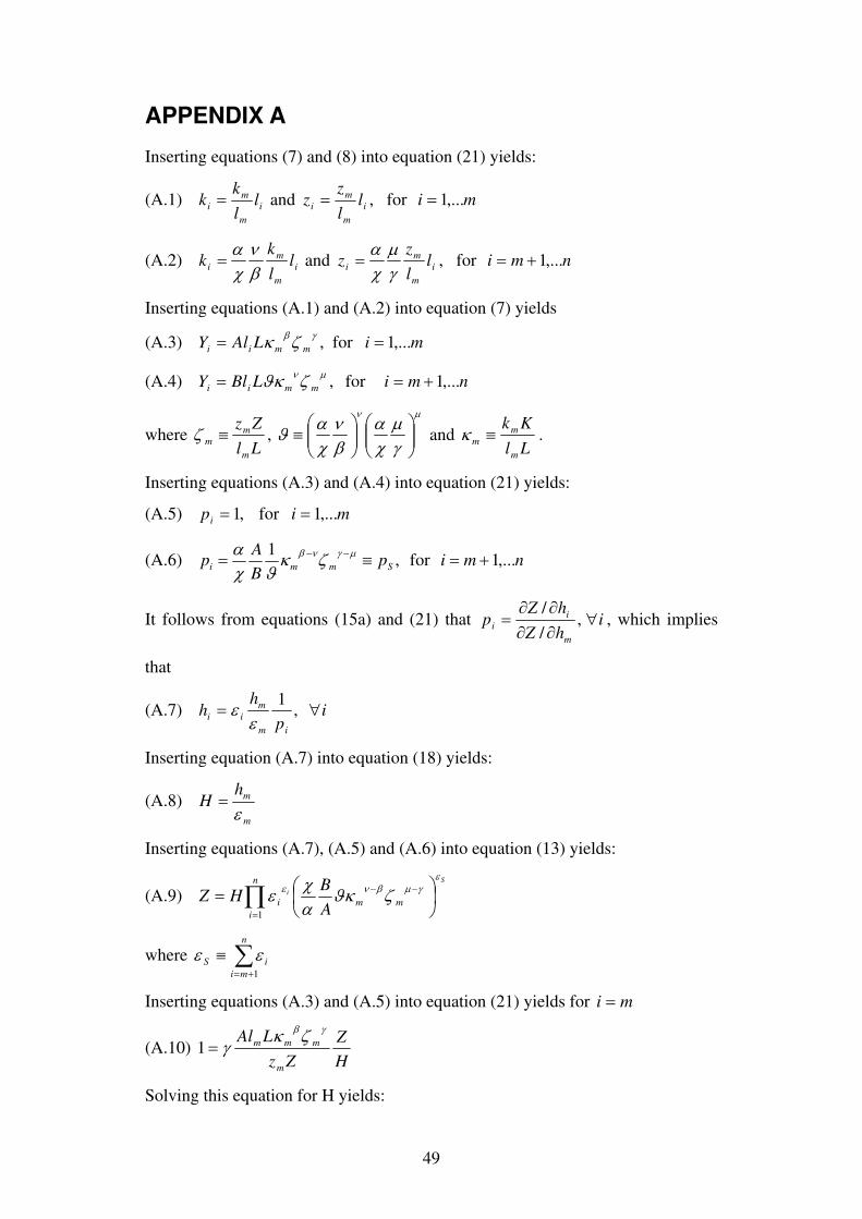
49
APPENDIX A
Inserting equations (7) and (8) into equation (21) yields:
(A.1) i
m
m
i ll
kk = and i
m
m
i ll
zz = , for mi ,...1=
(A.2) i
m
m
i ll
kk
βν
χα
= and i
m
m
i ll
zz
γμ
χα
= , for nmi ,...1+=
Inserting equations (A.1) and (A.2) into equation (7) yields
(A.3) miLAlY mmii ,...1for, == γβζκ
(A.4) nmiLBlY mmii ,...1for, +== μνζϑκ
where Ll
Zz
m
m
m ≡ζ ,
μν
γμ
χα
βν
χαϑ ⎟⎟
⎠
⎞⎜⎜⎝
⎛⎟⎟⎠
⎞⎜⎜⎝
⎛≡ and
Ll
Kk
m
m
m ≡κ .
Inserting equations (A.3) and (A.4) into equation (21) yields:
(A.5) mipi ,...1for ,1 ==
(A.6) nmipB
Ap Smmi ,...1for,
1+=≡= −− μγνβ ζκ
ϑχα
It follows from equations (15a) and (21) that ihZ
hZp
m
i
i ∀∂∂∂∂
= ,/
/, which implies
that
(A.7) ip
hh
im
m
ii ∀= ,1
εε
Inserting equation (A.7) into equation (18) yields:
(A.8) m
mhH
ε=
Inserting equations (A.7), (A.5) and (A.6) into equation (13) yields:
(A.9) ∏=
−− ⎟⎠⎞
⎜⎝⎛=
n
i
mmi
S
i
A
BHZ
1
εγμβνε ζϑκ
αχε
where ∑+=
≡n
mi
iS
1
εε
Inserting equations (A.3) and (A.5) into equation (21) yields for mi =
(A.10) H
Z
Zz
LAl
m
mmm
γβζκγ=1
Solving this equation for H yields:
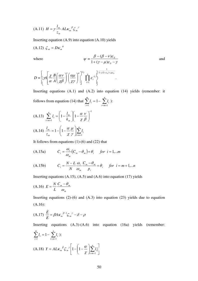
50
(A.11) γβζκγ mm
m
m ALz
lH =
Inserting equation (A.9) into equation (A.10) yields
(A.12) ψκζ mm D=
where γεμγ
ενββψ
−−+−−
≡S
S
)(1
)( and
SS
i
Sn
i
iA
BAD
μεεγε
εμν
εχγαμ
χβαν
αχγ
−−−
= ⎪⎭
⎪⎬⎫
⎪⎩
⎪⎨⎧
⎥⎥⎦
⎤
⎢⎢⎣
⎡⎟⎟⎠
⎞⎜⎜⎝
⎛⎟⎟⎠
⎞⎜⎜⎝
⎛≡ ∏
)1(1
1
1
.
Inserting equations (A.1) and (A.2) into equation (14) yields (remember: it
follows from equation (14) that ∑∑+==
−=n
mi
i
m
i
i ll11
1 ):
(A.13)
1
1
11
−
+=⎟⎟⎠
⎞⎜⎜⎝
⎛−⎟⎟
⎠
⎞⎜⎜⎝
⎛−=∑ β
νχαn
mi m
m
ik
ll
(A.14) ∑+=
⎟⎟⎠
⎞⎜⎜⎝
⎛−−=
n
mi
i
m
m lz
l
1
11γμ
χα
It follows from equations (1)-(6) and (22) that
(A.15a) ( ) miforCC imm
m
i
i ,...1=+−= θθωω
(A.15b) nmiforp
C
N
LNC i
i
mm
m
i
i ,...1+=+−−
= θθ
ωω
Inserting equations (A.15), (A.5) and (A.6) into equation (17) yields
(A.16) m
mmC
L
NE
ωθ−
=
Inserting equations (2)-(6) and (A.3) into equation (23) yields due to equation
(A.16):
(A.17) ρδζκβ γβ −−= −mmA
E
E 1&
Inserting equations (A.3)-(A.6) into equation (16a) yields (remember:
∑∑+==
−=n
mi
i
m
i
i ll11
1 ):
(A.18) ⎥⎦
⎤⎢⎣
⎡⎟⎟⎠
⎞⎜⎜⎝
⎛−−= ∑
+=
n
mi
imm lALY1
11χαζκ γβ
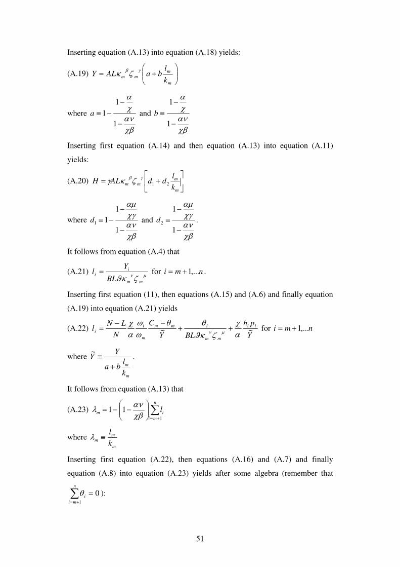
51
Inserting equation (A.13) into equation (A.18) yields:
(A.19) ⎟⎟⎠
⎞⎜⎜⎝
⎛+=
m
m
mmk
lbaALY
γβζκ
where
χβανχα
−
−−≡
1
1
1a and
χβανχα
−
−≡
1
1
b
Inserting first equation (A.14) and then equation (A.13) into equation (A.11)
yields:
(A.20) ⎥⎦
⎤⎢⎣
⎡+=
m
mmm
k
lddALH 21
γβζκγ
where
χβανχγαμ
−
−−≡
1
1
11d and
χβανχγαμ
−
−≡
1
1
2d .
It follows from equation (A.4) that
(A.21) μνζϑκ mm
i
iBL
Yl = for nmi ,...1+= .
Inserting first equation (11), then equations (A.15) and (A.6) and finally equation
(A.19) into equation (A.21) yields
(A.22) Y
ph
BLY
C
N
LNl ii
mm
imm
m
i
i ~~ αχ
ζϑκθθ
ωω
αχ
μν ++−−
= for nmi ,...1+=
where
m
m
k
lba
YY
+≡~
.
It follows from equation (A.13) that
(A.23) ∑+=
⎟⎟⎠
⎞⎜⎜⎝
⎛−−=
n
mi
im l1
11χβανλ
where m
mm
k
l≡λ
Inserting first equation (A.22), then equations (A.16) and (A.7) and finally
equation (A.8) into equation (A.23) yields after some algebra (remember that
∑+=
=n
mi
i
1
0θ ):
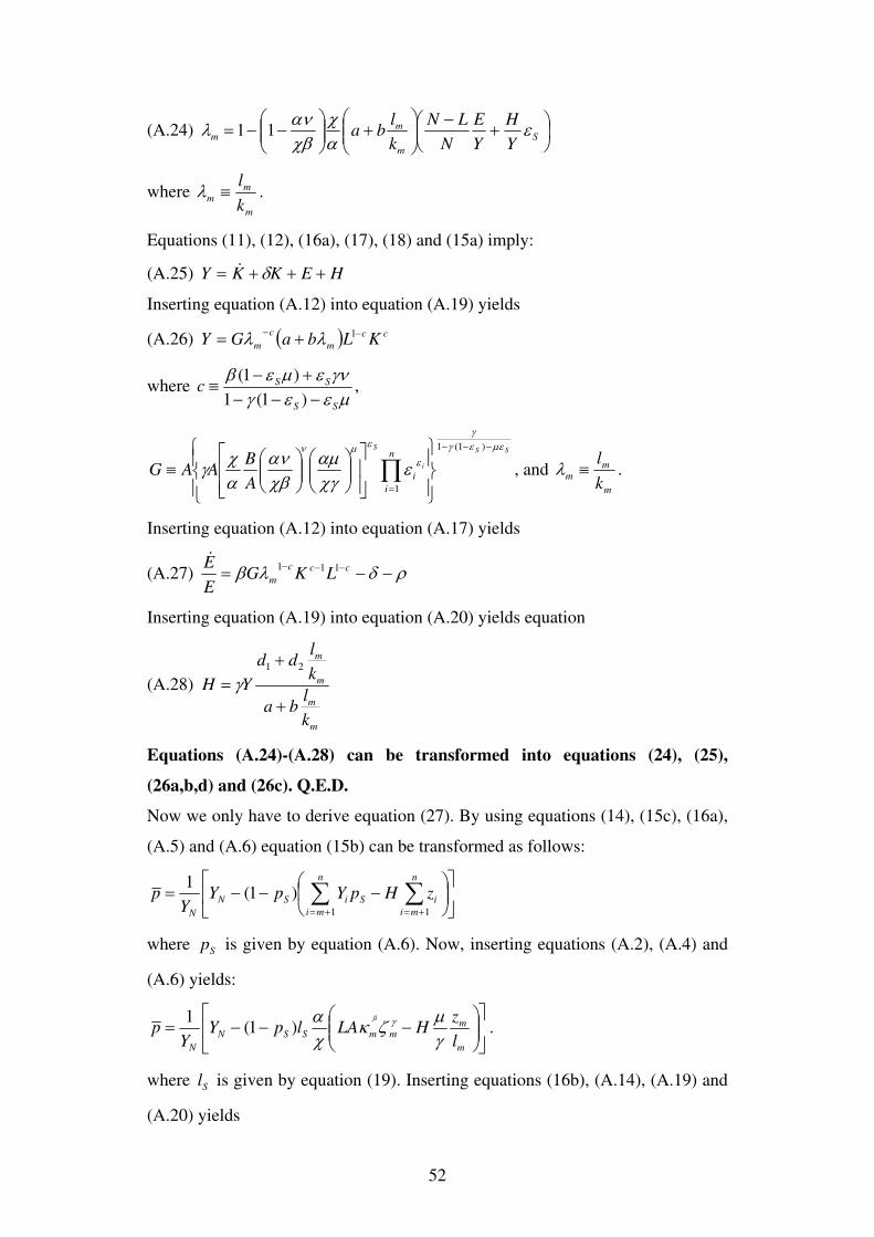
52
(A.24) ⎟⎠⎞
⎜⎝⎛ +
−⎟⎟⎠
⎞⎜⎜⎝
⎛+⎟⎟
⎠
⎞⎜⎜⎝
⎛−−= S
m
mm
Y
H
Y
E
N
LN
k
lba ε
αχ
χβανλ 11
where m
mm
k
l≡λ .
Equations (11), (12), (16a), (17), (18) and (15a) imply:
(A.25) HEKKY +++= δ&
Inserting equation (A.12) into equation (A.19) yields
(A.26) ( ) cc
m
c
m KLbaGY−− += 1λλ
where μεεγγνεμεβ
SS
SSc−−−+−
≡)1(1
)1(,
SS
i
Sn
i
iA
BAAG
μεεγγ
ε
εμν
εχγαμ
χβαν
αχγ
−−−
= ⎪⎭
⎪⎬⎫
⎪⎩
⎪⎨⎧
⎥⎥⎦
⎤
⎢⎢⎣
⎡⎟⎟⎠
⎞⎜⎜⎝
⎛⎟⎟⎠
⎞⎜⎜⎝
⎛≡ ∏
)1(1
1
, and m
mm
k
l≡λ .
Inserting equation (A.12) into equation (A.17) yields
(A.27) ρδλβ −−= −−− ccc
m LKGE
E 111&
Inserting equation (A.19) into equation (A.20) yields equation
(A.28)
m
m
m
m
k
lba
k
ldd
YH
+
+=
21
γ
Equations (A.24)-(A.28) can be transformed into equations (24), (25),
(26a,b,d) and (26c). Q.E.D.
Now we only have to derive equation (27). By using equations (14), (15c), (16a),
(A.5) and (A.6) equation (15b) can be transformed as follows:
⎥⎦
⎤⎢⎣
⎡⎟⎠
⎞⎜⎝
⎛−−−= ∑ ∑
+= +=
n
mi
n
mi
iSiSN
N
zHpYpYY
p1 1
)1(1
where Sp is given by equation (A.6). Now, inserting equations (A.2), (A.4) and
(A.6) yields:
⎥⎦
⎤⎢⎣
⎡⎟⎟⎠
⎞⎜⎜⎝
⎛−−−=
m
mmmSSN
N l
zHLAlpY
Yp
ß
γμζκ
χα γ)1(
1.
where Sl is given by equation (19). Inserting equations (16b), (A.14), (A.19) and
(A.20) yields
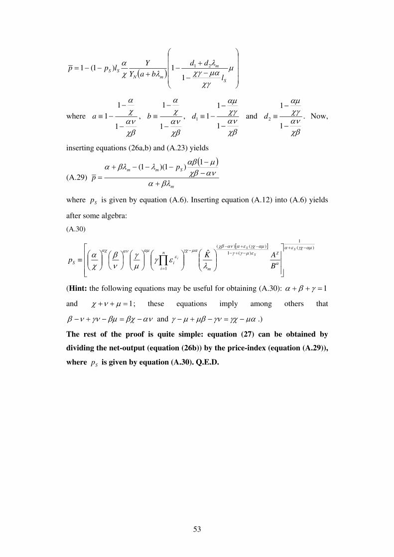
53
( )⎟⎟⎟⎟
⎠
⎞
⎜⎜⎜⎜
⎝
⎛
−−
+−
+−−= μ
χγμαχγλ
λχα
S
m
mN
SS
l
dd
baY
Ylpp
1
1)1(1 21
where
χβανχα
−
−−≡
1
1
1a ,
χβανχα
−
−≡
1
1
b ,
χβανχγαμ
−
−−≡
1
1
11d and
χβανχγαμ
−
−≡
1
1
2d . Now,
inserting equations (26a,b) and (A.23) yields
(A.29)
( )
m
Smm p
pβλα
ανχβμαβλβλα
+−−
−−−+=
1)1)(1(
where Sp is given by equation (A.6). Inserting equation (A.12) into (A.6) yields
after some algebra:
(A.30)
[ ] )(
1
)(1
)()(
1
ˆαμγχεα
α
χεμγγαμγχεαανχβ
μαγχε
αμαναχ
λεγ
μγ
νβ
χα
−+−+−
−+−−
= ⎥⎥⎥
⎦
⎤
⎢⎢⎢
⎣
⎡
⎟⎟⎠
⎞⎜⎜⎝
⎛⎟⎟⎠
⎞⎜⎜⎝
⎛⎟⎟⎠
⎞⎜⎜⎝
⎛⎟⎠⎞
⎜⎝⎛
⎟⎟⎠
⎞⎜⎜⎝
⎛≡ ∏
S
S
S
i
B
AKp
m
n
i
iS
(Hint: the following equations may be useful for obtaining (A.30): 1=++ γβα
and 1=++ μνχ ; these equations imply among others that
ανβχβμγννβ −=−+− and μαγχγνμβμγ −=−+− .)
The rest of the proof is quite simple: equation (27) can be obtained by
dividing the net-output (equation (26b)) by the price-index (equation (A.29)),
where Sp is given by equation (A.30). Q.E.D.

54
APPENDIX B
Equations (A.7), (A.8), (A.16) and (A.22) from APPENDIX A and equations
(5a,b) and (19) imply equation (29).
Equation (28) can be derived in the same way as equation (29).
Equations (A.5), (A.6), (A.15a,b), (A.16) from APPENDIX A and equations
(5a,b) and (20) imply equations (30) and (31).
For a proof of equations (32) and (33) see APPENDIX A equations (A.1) and
(A.2).
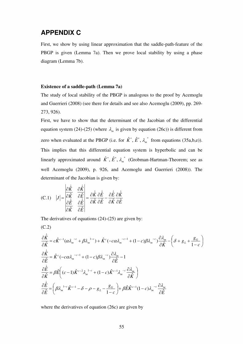
55
APPENDIX C
First, we show by using linear approximation that the saddle-path-feature of the
PBGP is given (Lemma 7a). Then we prove local stability by using a phase
diagram (Lemma 7b).
Existence of a saddle-path (Lemma 7a)
The study of local stability of the PBGP is analogous to the proof by Acemoglu
and Guerrieri (2008) (see there for details and see also Acemoglu (2009), pp. 269-
273, 926).
First, we have to show that the determinant of the Jacobian of the differential
equation system (24)-(25) (where mλ is given by equation (26c)) is different from
zero when evaluated at the PBGP (i.e. for *** ,ˆ,ˆ
mEK λ from equations (35a,b,e)).
This implies that this differential equation system is hyperbolic and can be
linearly approximated around *** ,ˆ,ˆ
mEK λ (Grobman-Hartman-Theorem; see as
well Acemoglu (2009), p. 926, and Acemoglu and Guerrieri (2008)). The
determinant of the Jacobian is given by:
(C.1) E
K
K
E
E
E
K
K
E
E
K
E
E
K
K
K
Jˆ
ˆ
ˆ
ˆ
ˆ
ˆ
ˆ
ˆ
ˆ
ˆ
ˆ
ˆ
ˆ
ˆ
ˆ
ˆ
∂∂
∂∂
−∂∂
∂∂
=
∂∂
∂∂
∂∂
∂∂
=&&&&
&&
&&
The derivatives of equations (24)-(25) are given by:
(C.2)
EcKE
c
ggK
E
E
KKcKcE
K
E
EccK
E
K
c
gg
KccKKc
K
K
mc
m
cGL
cc
m
mc
m
cc
m
c
mc
m
c
m
c
GL
mc
m
c
m
cc
m
c
m
c
ˆ)1(ˆˆ
1ˆ
ˆ
ˆ
ˆˆ)1(ˆ)1(ˆ
ˆ
ˆ
1ˆ
))1((ˆˆ
ˆ
1ˆ))1((ˆ)(ˆ
ˆ
ˆ
111
112
1
111
∂∂
−+⎟⎠⎞
⎜⎝⎛
−−−−−=
∂∂
⎟⎠⎞
⎜⎝⎛
∂∂
−+−=∂∂
−∂∂
−+−=∂∂
⎟⎠⎞
⎜⎝⎛
−++−
∂∂
−+−++=∂∂
−−−−
−−−−
−−−
−−−−−−
λλβρδβλ
λλλβ
λβλαλ
δλβλαλβλαλ
&
&
&
&
where the derivatives of equation (26c) are given by
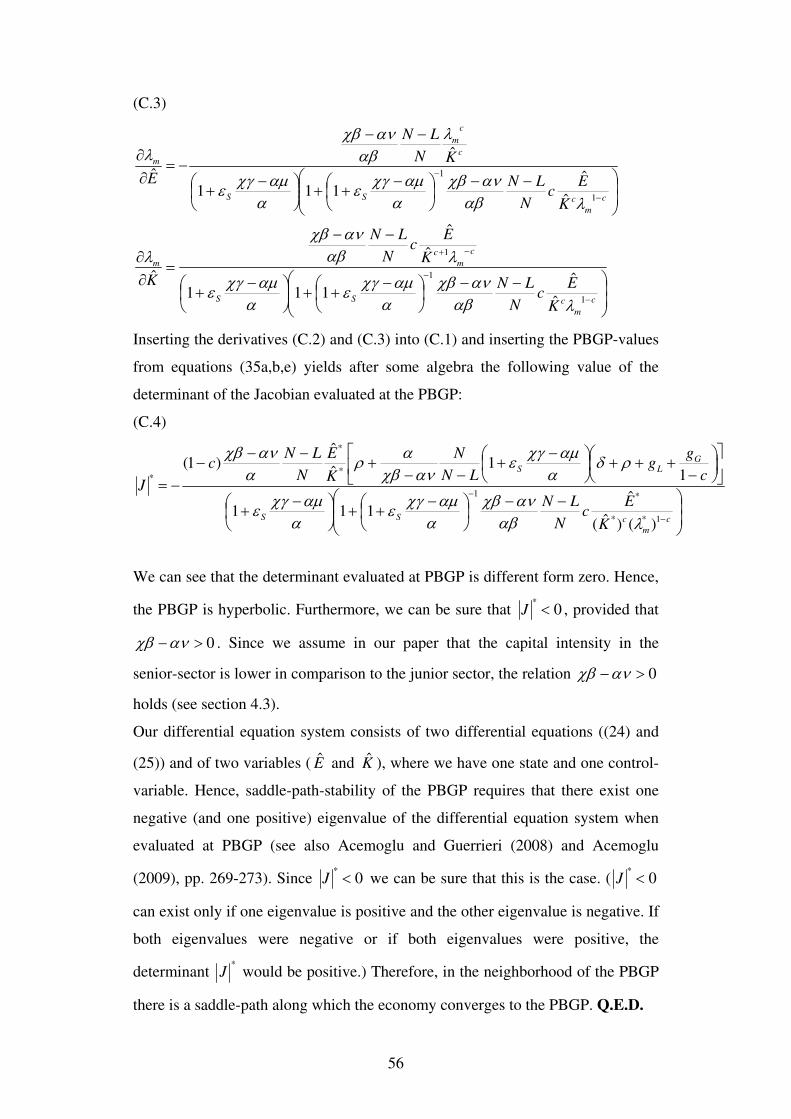
56
(C.3)
⎟⎟⎠
⎞⎜⎜⎝
⎛ −−⎟⎠⎞
⎜⎝⎛ −++⎟
⎠⎞
⎜⎝⎛ −+
−−
=∂∂
⎟⎟⎠
⎞⎜⎜⎝
⎛ −−⎟⎠⎞
⎜⎝⎛ −++⎟
⎠⎞
⎜⎝⎛ −+
−−
−=∂∂
−
−
−+
−
−
c
m
cSS
c
m
c
m
c
m
cSS
c
c
m
m
K
Ec
N
LN
K
Ec
N
LN
K
K
Ec
N
LN
KN
LN
E
1
1
1
1
1
ˆ
ˆ111
ˆ
ˆ
ˆ
ˆ
ˆ111
ˆ
ˆ
λαβανχβ
ααμχγε
ααμχγε
λαβανχβ
λ
λαβανχβ
ααμχγε
ααμχγε
λαβ
ανχβλ
Inserting the derivatives (C.2) and (C.3) into (C.1) and inserting the PBGP-values
from equations (35a,b,e) yields after some algebra the following value of the
determinant of the Jacobian evaluated at the PBGP:
(C.4)
⎟⎟⎠
⎞⎜⎜⎝
⎛ −−⎟⎠⎞
⎜⎝⎛ −++⎟
⎠⎞
⎜⎝⎛ −+
⎥⎦
⎤⎢⎣
⎡⎟⎠⎞
⎜⎝⎛
−+++⎟
⎠⎞
⎜⎝⎛ −+
−−+
−−−
−=
−
−
c
m
cSS
GLS
K
Ec
N
LN
c
gg
LN
N
K
E
N
LNc
J
1**
*1
*
*
*
)()ˆ(
ˆ111
11
ˆ
ˆ)1(
λαβανχβ
ααμχγε
ααμχγε
ρδααμχγε
ανχβαρ
αανχβ
We can see that the determinant evaluated at PBGP is different form zero. Hence,
the PBGP is hyperbolic. Furthermore, we can be sure that 0* <J , provided that
0>−ανχβ . Since we assume in our paper that the capital intensity in the
senior-sector is lower in comparison to the junior sector, the relation 0>−ανχβ
holds (see section 4.3).
Our differential equation system consists of two differential equations ((24) and
(25)) and of two variables ( E and K ), where we have one state and one control-
variable. Hence, saddle-path-stability of the PBGP requires that there exist one
negative (and one positive) eigenvalue of the differential equation system when
evaluated at PBGP (see also Acemoglu and Guerrieri (2008) and Acemoglu
(2009), pp. 269-273). Since 0* <J we can be sure that this is the case. ( 0
* <J
can exist only if one eigenvalue is positive and the other eigenvalue is negative. If
both eigenvalues were negative or if both eigenvalues were positive, the
determinant *
J would be positive.) Therefore, in the neighborhood of the PBGP
there is a saddle-path along which the economy converges to the PBGP. Q.E.D.
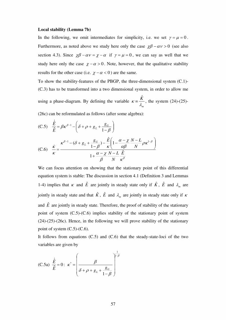
57
Local stability (Lemma 7b)
In the following, we omit intermediates for simplicity, i.e. we set 0== μγ .
Furthermore, as noted above we study here only the case 0>−ανχβ (see also
section 4.3). Since αχανχβ −=− if 0== μγ , we can say as well that we
study here only the case 0>−αχ . Note, however, that the qualitative stability
results for the other case (i.e. 0<−αχ ) are the same.
To show the stability-features of the PBGP, the three-dimensional system (C.1)-
(C.3) has to be transformed into a two dimensional system, in order to allow me
using a phase-diagram. By defining the variable m
K
λκ
ˆ≡ , the system (24)-(25)-
(26c) can be reformulated as follows (after some algebra):
(C.5) ⎟⎟⎠
⎞⎜⎜⎝
⎛−
+++−= −
βρδβκ β
1ˆ
ˆ1 G
L
gg
E
E&
(C.6)
β
ββ
κβχα
ρκαβ
χακβ
δκ
κκ
E
N
LN
N
LNEgg G
L
ˆ1
1ˆ
)1
( 11
−−+
⎟⎟⎠
⎞⎜⎜⎝
⎛ −−−−
−++−
=
−−
&
We can focus attention on showing that the stationary point of this differential
equation system is stable: The discussion in section 4.1 (Definition 3 and Lemmas
1-4) implies that κ and E are jointly in steady state only if K , E and mλ are
jointly in steady state and that K , E and mλ are jointly in steady state only if κ
and E are jointly in steady state. Therefore, the proof of stability of the stationary
point of system (C.5)-(C.6) implies stability of the stationary point of system
(24)-(25)-(26c). Hence, in the following we will prove stability of the stationary
point of system (C.5)-(C.6).
It follows from equations (C.5) and (C.6) that the steady-state-loci of the two
variables are given by
(C.5a)
β
βρδ
βκ
−
⎟⎟⎟⎟
⎠
⎞
⎜⎜⎜⎜
⎝
⎛
−+++
==
1
1
*
1
:0ˆ
ˆ
GL
ggE
E&
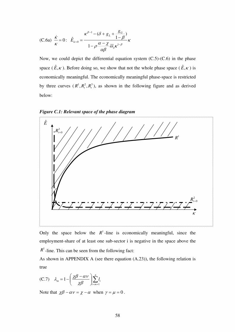
58
(C.6a) κκω
αβχαρ
βδκ
κκ
β
β
κ−
−
= −−
−++−
==1
1
0
1
)1
(ˆ:0
n
GL
gg
E &
&
Now, we could depict the differential equation system (C.5)-(C.6) in the phase
space ( κ,E ). Before doing so, we show that not the whole phase space ( κ,E ) is
economically meaningful. The economically meaningful phase-space is restricted
by three curves ( 321 ,, tt RRR ), as shown in the following figure and as derived
below:
Figure C.1: Relevant space of the phase diagram
Only the space below the 1R -line is economically meaningful, since the
employment-share of at least one sub-sector i is negative in the space above the
1R -line. This can be seen from the following fact:
As shown in APPENDIX A (see there equation (A.23)), the following relation is
true
(C.7) ∑+=
⎟⎟⎠
⎞⎜⎜⎝
⎛ −−=
n
mi
im l1
1χβανχβλ
Note that αχανχβ −=− when 0== μγ .
κ
E
1R
3
0=tR
2
0=tR
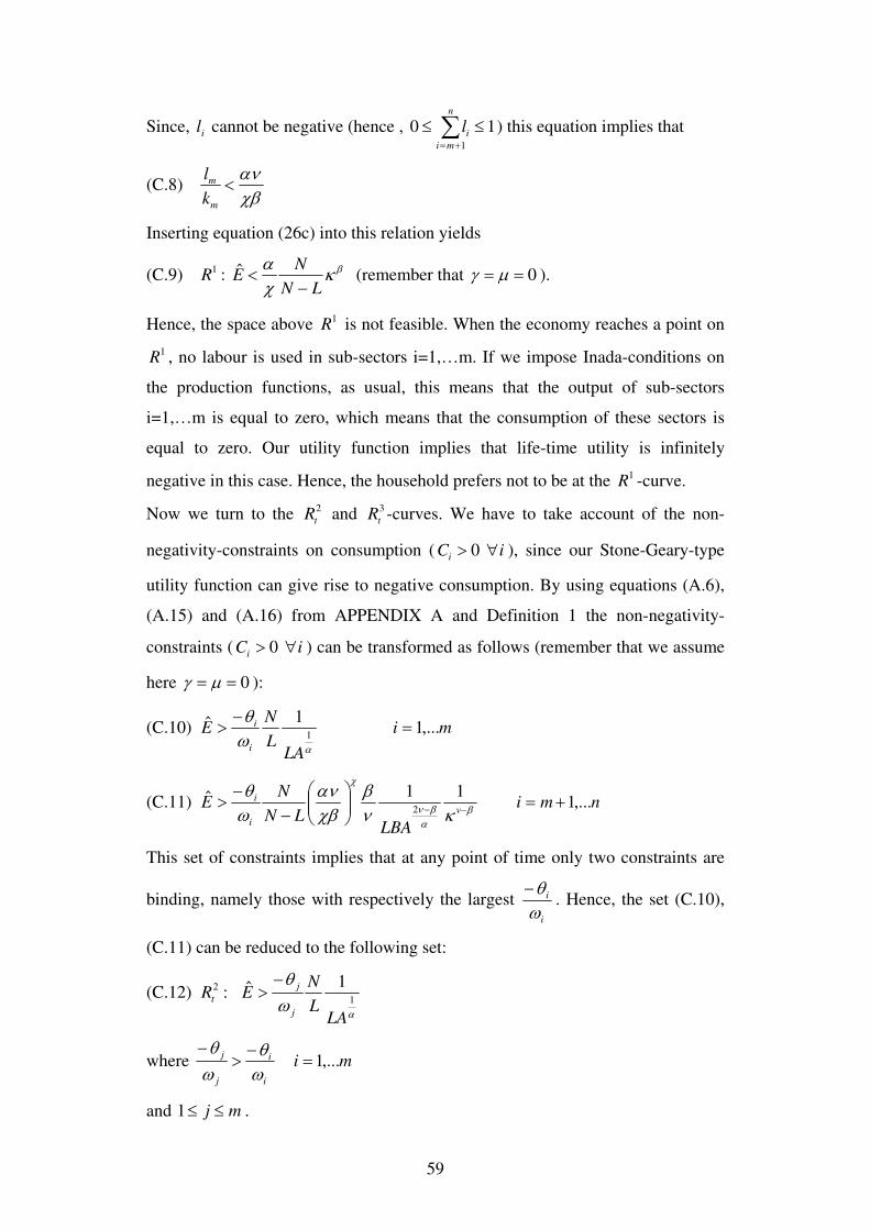
59
Since, il cannot be negative (hence , 101
≤≤ ∑+=
n
mi
il ) this equation implies that
(C.8) χβαν
<m
m
k
l
Inserting equation (26c) into this relation yields
(C.9) βκχα
LN
NER
−<ˆ:1 (remember that 0== μγ ).
Hence, the space above 1R is not feasible. When the economy reaches a point on
1R , no labour is used in sub-sectors i=1,…m. If we impose Inada-conditions on
the production functions, as usual, this means that the output of sub-sectors
i=1,…m is equal to zero, which means that the consumption of these sectors is
equal to zero. Our utility function implies that life-time utility is infinitely
negative in this case. Hence, the household prefers not to be at the 1R -curve.
Now we turn to the 2
tR and 3
tR -curves. We have to take account of the non-
negativity-constraints on consumption ( iCi ∀> 0 ), since our Stone-Geary-type
utility function can give rise to negative consumption. By using equations (A.6),
(A.15) and (A.16) from APPENDIX A and Definition 1 the non-negativity-
constraints ( iCi ∀> 0 ) can be transformed as follows (remember that we assume
here 0== μγ ):
(C.10) mi
LAL
NE
i
i ,...11ˆ
1=
−>
αωθ
(C.11) nmi
LBALN
NE
v
i
i ,...111ˆ
2+=⎟⎟
⎠
⎞⎜⎜⎝
⎛−
−> −− β
αβν
χ
κνβ
χβαν
ωθ
This set of constraints implies that at any point of time only two constraints are
binding, namely those with respectively the largest i
i
ωθ−
. Hence, the set (C.10),
(C.11) can be reduced to the following set:
(C.12)
αωθ
1
2 1ˆ:
LAL
NER
j
j
t
−>
where mii
i
j
j,...1=
−>
−ωθ
ωθ
and mj ≤≤1 .
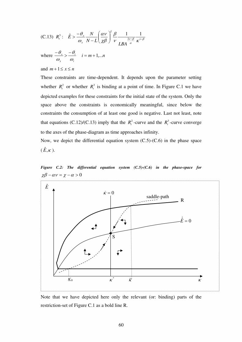
60
(C.13) βαβν
χ
κνβ
χβαν
ωθ
−−⎟⎟⎠
⎞⎜⎜⎝
⎛−
−>
v
x
xt
LBALN
NER
11ˆ:2
3
where nmii
i
x
x ,...1+=−
>−
ωθ
ωθ
and nxm ≤≤+1
These constraints are time-dependent. It depends upon the parameter setting
whether 2
tR or whether 3
tR is binding at a point of time. In Figure C.1 we have
depicted examples for these constraints for the initial state of the system. Only the
space above the constraints is economically meaningful, since below the
constraints the consumption of at least one good is negative. Last not least, note
that equations (C.12)/(C.13) imply that the 2
tR -curve and the 3
tR -curve converge
to the axes of the phase-diagram as time approaches infinity.
Now, we depict the differential equation system (C.5)-(C.6) in the phase space
( κ,E ).
Figure C.2: The differential equation system (C.5)-(C.6) in the phase-space for
0>−=− αχανχβ
Note that we have depicted here only the relevant (or: binding) parts of the
restriction-set of Figure C.1 as a bold line R.
κ
E
*κ
0=κ&
0ˆ =E&
S
saddle-path
κ0κ
R
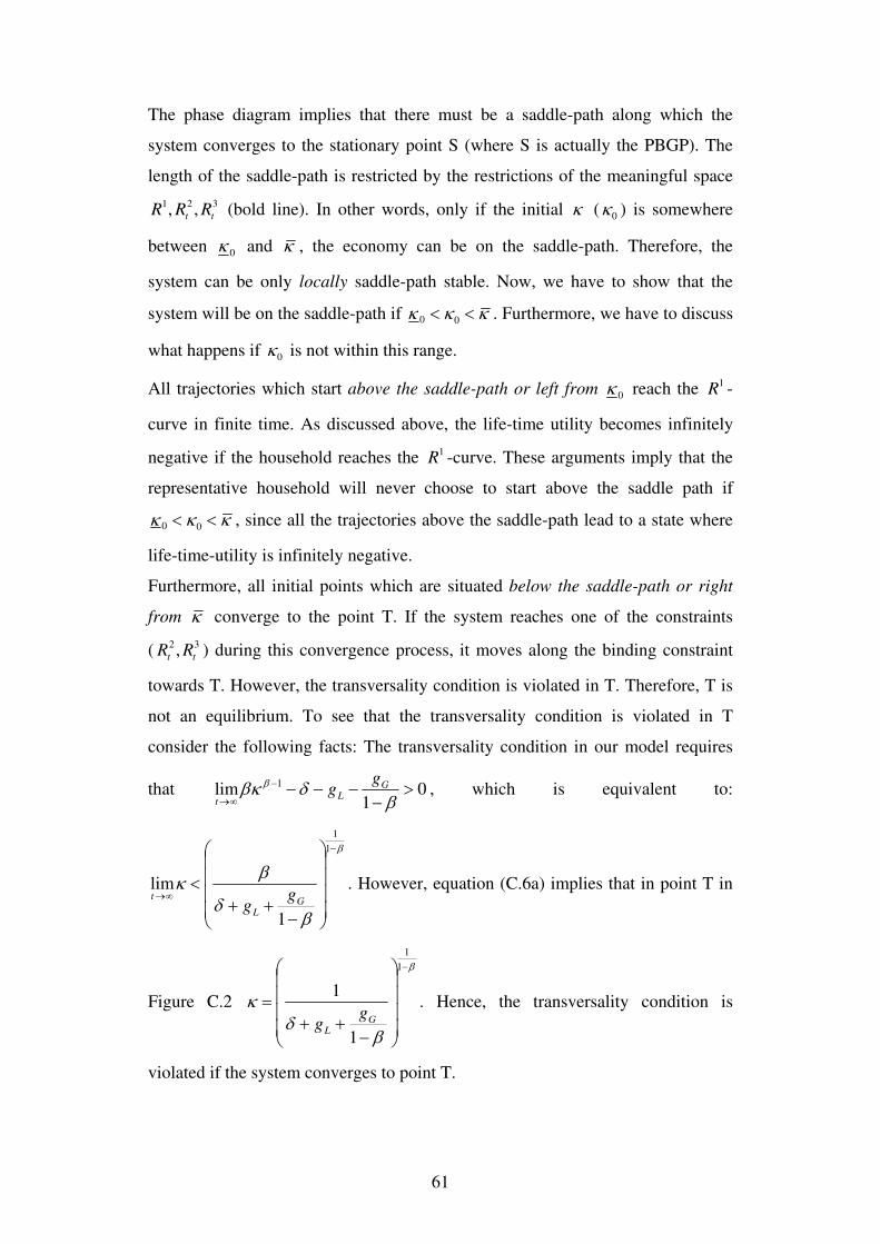
61
The phase diagram implies that there must be a saddle-path along which the
system converges to the stationary point S (where S is actually the PBGP). The
length of the saddle-path is restricted by the restrictions of the meaningful space
321 ,, tt RRR (bold line). In other words, only if the initial κ ( 0κ ) is somewhere
between 0κ and κ , the economy can be on the saddle-path. Therefore, the
system can be only locally saddle-path stable. Now, we have to show that the
system will be on the saddle-path if κκκ << 00 . Furthermore, we have to discuss
what happens if 0κ is not within this range.
All trajectories which start above the saddle-path or left from 0κ reach the 1R -
curve in finite time. As discussed above, the life-time utility becomes infinitely
negative if the household reaches the 1R -curve. These arguments imply that the
representative household will never choose to start above the saddle path if
κκκ << 00 , since all the trajectories above the saddle-path lead to a state where
life-time-utility is infinitely negative.
Furthermore, all initial points which are situated below the saddle-path or right
from κ converge to the point T. If the system reaches one of the constraints
( 32 , tt RR ) during this convergence process, it moves along the binding constraint
towards T. However, the transversality condition is violated in T. Therefore, T is
not an equilibrium. To see that the transversality condition is violated in T
consider the following facts: The transversality condition in our model requires
that 01
lim 1 >−
−−−−
∞→ βδβκ β G
Lt
gg , which is equivalent to:
β
βδ
βκ
−
∞→
⎟⎟⎟⎟
⎠
⎞
⎜⎜⎜⎜
⎝
⎛
−++
<
1
1
1
limG
L
t gg
. However, equation (C.6a) implies that in point T in
Figure C.2
β
βδ
κ
−
⎟⎟⎟⎟
⎠
⎞
⎜⎜⎜⎜
⎝
⎛
−++
=
1
1
1
1
GL
gg
. Hence, the transversality condition is
violated if the system converges to point T.
62
Overall, we know that, if κκκ << 00 , the household always decides to be on the
saddle-path. Hence, we know that for κκκ << 00 the economy converges to the
PBGP. In this sense, the PBGP is locally stable (within the range κκκ << 00 ).
If the initial capital is to small ( 00 κκ < ), the economy converges to a state
where some existence minima are not satisfied (curve 1R ) and, thus, utility
becomes infinitely negative. This may be interpreted as a development trap. On
the other hand, if initial capital-level is too large ( κκ >0 ), all trajectories violate
the transversality condition. Therefore, in this case, the representative
household must waste a part of its initial capital to come into the feasible area
( κκκ << 00 ).
Q.E.D.

63
APPENDIX D
Due to equation (16c) we know that
(D.1) *
**
**
*
p
Y
N
LN
pp
N
LN
Y
N
LN
GDP
NN
⎟⎠⎞
⎜⎝⎛ −∂
∂−
⎟⎠⎞
⎜⎝⎛ −∂
∂
=⎟⎠⎞
⎜⎝⎛ −∂
∂
Equation (38) can be obtained by inserting equation (A.29) from APPENDIX A
and equation (35d) into equation (D.1). Hints: Equation (A.30) from APPENDIX
A and equation (35a) imply that 0*
=⎟⎠⎞
⎜⎝⎛ −∂
∂
N
LN
pS . Furthermore, we used equation
(A.23) to transform *
mλ into *
Sl .