Embed Size (px)
Citation preview
1
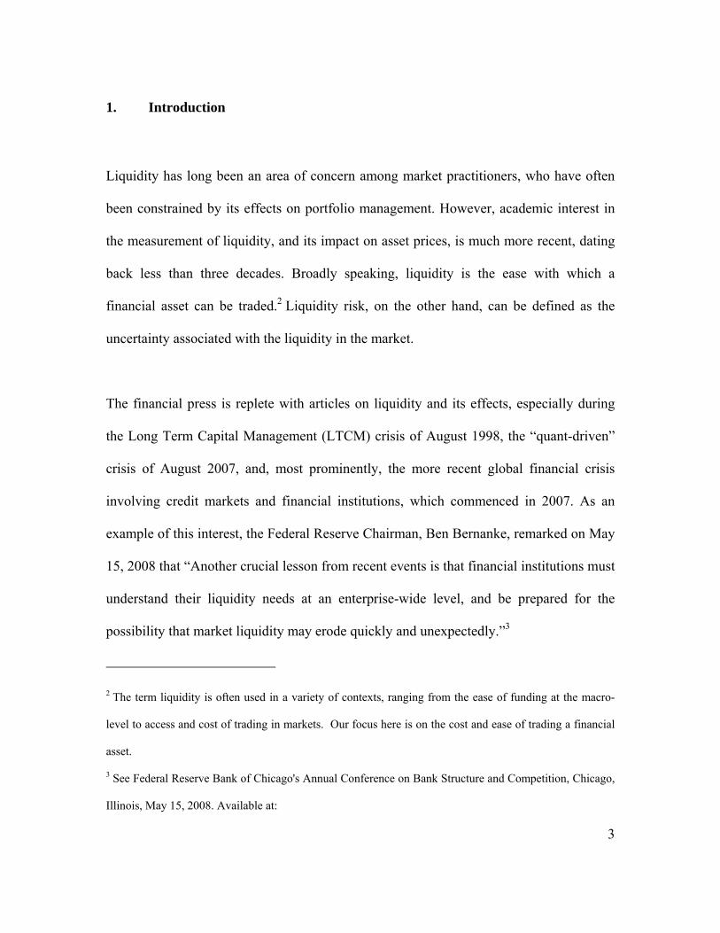
LIQUIDITY AND PORTFOLIO MANAGEMENT: AN INTRA-DAY ANALYSIS
Joseph Cherian*, Sriketan Mahanti† and Marti G. Subrahmanyam‡1
First Draft: November 13, 2008
This Draft: September 8, 2011
Abstract
A recent area of interest among both financial economists and market practitioners has
been the measurement of liquidity and its impact on asset prices. Broadly speaking,
liquidity is the ease with which a financial asset can be traded. Liquidity risk, on the other
hand, can be defined in terms of the uncertainty associated with the measure of liquidity.
Using the ILLIQ measure first proposed by Amihud (2002) as the basis, we provide
empirical evidence in support of a more-refined version of this liquidity measure based
on intra-day data. Our results strongly validate the notion that liquidity affects financial
market performance, and, as a consequence, have implications for both portfolio
construction and risk management. Our approach permits us to identify different liquidity
regimes in financial markets by measuring the relation between aggregate market
liquidity and the market’s pricing of liquidity risk. It hence has the potential to displace
JEL Classification G 100 (General Financial Markets). We are grateful to Larry Pohlman and Wenjin Kang for helpful suggestions. We acknowledge, with thanks, comments from participants at the Boston Security Analysts Society (BSAS) and QWAFAFEW meetings in Boston, MA and the JOIM Spring Conference in San Francisco, CA. We thank Orissa Group, Inc. for providing us the data used in the study. *email: [email protected]; Tel: +65 6516 5991. Joseph Cherian is on the faculty at the National University of Singapore Business School. †email: [email protected]; Tel: +1 508 517 2636. Sriketan Mahanti was formerly a Managing Director at the Orissa Group. ‡email: [email protected]; Tel: +1 212 998 0348. Marti Subrahmanyam is on the faculty at the Stern School of Business, New York University.

2
other traditional indirect proxies of liquidity in standard asset pricing tests. Finally, by
using the liquidity measures developed here, and market instruments with relatively low
transaction and liquidity costs, we derive the rationale for, and present the results of, an
easily-implementable and profitable liquidity-driven trading strategy.
3
1. Introduction
Liquidity has long been an area of concern among market practitioners, who have often
been constrained by its effects on portfolio management. However, academic interest in
the measurement of liquidity, and its impact on asset prices, is much more recent, dating
back less than three decades. Broadly speaking, liquidity is the ease with which a
financial asset can be traded.2 Liquidity risk, on the other hand, can be defined as the
uncertainty associated with the liquidity in the market.
The financial press is replete with articles on liquidity and its effects, especially during
the Long Term Capital Management (LTCM) crisis of August 1998, the “quant-driven”
crisis of August 2007, and, most prominently, the more recent global financial crisis
involving credit markets and financial institutions, which commenced in 2007. As an
example of this interest, the Federal Reserve Chairman, Ben Bernanke, remarked on May
15, 2008 that “Another crucial lesson from recent events is that financial institutions must
understand their liquidity needs at an enterprise-wide level, and be prepared for the
possibility that market liquidity may erode quickly and unexpectedly.”3
2 The term liquidity is often used in a variety of contexts, ranging from the ease of funding at the macro-
level to access and cost of trading in markets. Our focus here is on the cost and ease of trading a financial
asset.
3 See Federal Reserve Bank of Chicago's Annual Conference on Bank Structure and Competition, Chicago,
Illinois, May 15, 2008. Available at:

4
Academic interest in liquidity issues can be traced back to the classic paper by Amihud
and Mendelson (1986), which demonstrates that, for investors with a short horizon,
transaction costs are important, and liquid assets are likely to be the better investment,
despite being priced higher than their illiquid counterparts. However, for investors with
longer holding periods, transaction costs are less important, since they are amortized over
a longer period, and the illiquid asset may be the better investment since it has a lower
price, ceteris paribus. As a consequence, short-term investors would invest in the most
liquid securities, while long-term investors, such as pension funds and insurance
companies, can potentially use illiquid instruments to fund long-term liabilities and earn
the extra liquidity premium. This would lead to an equilibrium in which investors are
sorted into liquidity clienteles, based on their investment horizons. This concept has been
elaborated on in a number of papers in the literature, as documented in Amihud,
Mendelson and Pedersen (2005). We briefly discuss below a selected list of papers in the
literature that are directly related to our own research.4
In a paper on illiquidity, Amihud (2002) proposes a measure of price impact that is
intuitive and simple to implement. It is based on the λ measure of Kyle (1985), which
measures the marginal impact of price with respect to a unit of trading volume. More
http://www.federalreserve.gov/newsevents/speech/bernanke20080515a.htm
4 We do not attempt to survey the whole literature on the effects of liquidity on asset prices here. Please see
Amihud, Mendelson and Pedersen (2005) for a more comprehensive survey.
5
specifically, the Amihud measure, ILLIQ, is the average ratio of the absolute return in a
stock to its dollar trading volume in any given period, i.e.,
T
t t
t
V
r
T 1
||1 where rt is the daily
stock’s return, Vt is the trading volume in dollars during that day, and T is the number of
trading days during the time period.
In an equilibrium context with liquidity risk, Acharya and Pedersen (2005) derive a
liquidity-adjusted capital asset pricing model, in which the security’s equilibrium rate of
return depends on its expected liquidity as measured by the ILLIQ measure, as well as the
liquidity risks measured by the covariances of its returns with that of the market’s return
and liquidity costs. In addition, their model yields the result that investors are more
attracted to liquid securities when the market return is low. This result is broadly
consistent with the empirical findings of Hameed, Kang and Viswanathan (2007) who
document that negative market returns decrease stock liquidity for high volatility stocks,
especially during times of tightness in the funding market.
In the context of portfolio optimization, Lo, Petrov, and Wierzbicki (2003) explicitly
model liquidity into the portfolio construction process. Using mean-variance optimized
portfolios adjusted for liquidity in three distinct ways, Lo et al. find that portfolios “close
to each other” on the traditional mean-variance efficient frontier can differ substantially
in their liquidity characteristics. Their analysis also reveals that simple forms of liquidity
optimization can yield significant benefits in reducing a portfolio’s liquidity-risk
exposure, without sacrificing a great deal of expected return per unit of risk.

6
In our paper, we define, develop, and empirically test some measures of liquidity and
liquidity risk, both at the stock- and market-levels. Using the well-accepted ILLIQ
measure of liquidity, as defined first by Kyle (1985) and then operationalized by Amihud
(2002), as the basis, we provide empirical evidence that a more-refined version of this
liquidity measure, which uses intra-day data, strongly validates the notion that liquidity
affects financial market performance. As a consequence, it has direct implications for
both optimal portfolio construction and risk management.
This paper’s major contributions are manifold. First, to our knowledge, it is the first
paper to analyze intraday price returns and trading volume data for US stocks in order to
estimate financial market liquidity, both in terms of its level and its risk. Second, we
propose and employ a liquidity normalization factor, which substantially improves the
time-series characteristics of the liquidity measures. Our measure permits the
identification of different market liquidity regimes by using new transactions-based,
market-wide metrics of illiquidity. It measures the interaction between aggregate market
liquidity and the market’s pricing of liquidity risk. Third, the liquidity risk factor that
results from our analysis has the ability to displace other traditional indirect proxies of
liquidity, such as the Fama-French size factor (SMB), in standard asset pricing tests. Last,
but not least, by using the liquidity measures developed herein, we derive the rationale
for a profitable and implementable liquidity-driven trading strategy.
The paper is organized as follows. In Section 2, we develop the basic empirical model of
liquidity and liquidity risk that we use in our empirical analysis. We next formulate a
7
market-wide metric of illiquidity in Section 3 to represent fluctuations in aggregate
market liquidity. We test this metric in Section 4 to determine whether the illiquidity
measures developed have incremental explanatory power for equity returns relative to the
Fama and French three-factor model. Section 5 builds on the results of the previous
section to develop the rationale for a simple liquidity-based trading strategy, while
Section 6 concludes.
2. An Empirical Model of Liquidity Risk
2.1. The Illiquidity Measure
The first question one can ask in the context of liquidity and portfolio management is the
concept and measurement of liquidity. Although there are many aspects of liquidity, the
two most common types of measures used in practice are:
1. Funding Effect: This is the ease with which or availability to finance positions
over a short period (for example, as reflected in repo and reverse repo markets);
2. Transaction Effect: This is the ease with which positions can be created or
liquidated.
While the first effect reflects the broader market environment, the second directly relates
to an investor’s ability to create or liquidate positions without significantly affecting
prices: i.e., being able to buy or sell a security close to the prevailing market value. The
second measure is the one most commonly used by financial economists and market
participants, and the one we adopt in this paper.

8
Strictly speaking, Kyle’s notion on which Amihud’s measure is based, has to be
interpreted over a very short time interval, as it measures the price impact of individual
trades. Furthermore, from a trader’s perspective, liquidity is a short-term phenomenon,
and hence needs to be addressed over a short time interval. We therefore deliberately
model the liquidity factor, as well as the liquidity attributes of individual securities, in the
intra-day context.
The modeling of liquidity in the current paper follows a two-step process. In the first step,
we estimate the ease with which positions can be liquidated. This is the magnitude of
price movements resulting from a given order size, and is based on the Amihud (2002)
measure of illiquidity described above. We restrict our universe to U.S. domiciled
common stocks. In our model, each trading day is divided into 10 equal trading time
intervals, with each time interval being equal to 39 minutes. (The normal trading hours
for U.S. equity markets are between 9.30 am and 4 pm, a total of 390 minutes.) For each
security i, for a given time interval t (= 1 - 10, for each trading day in that particular
month), and month m (January 1993 through December 2009) we first compute the trade
volume weighted price as imtp , . The return for the trading interval is then given as , =
( imtp , - i
mtp ,1 ) / imtp ,1 , where i
mtp ,1 is the trade volume weighted price for the prior trading
interval within the same trading day. (The return is not defined for the first trading
interval within the day.) Hence, for each trading day, with 10 trading intervals, 9 (i.e., 2 -
10) return observations are computed. Defining imtV , as the dollar volume (in millions),
9
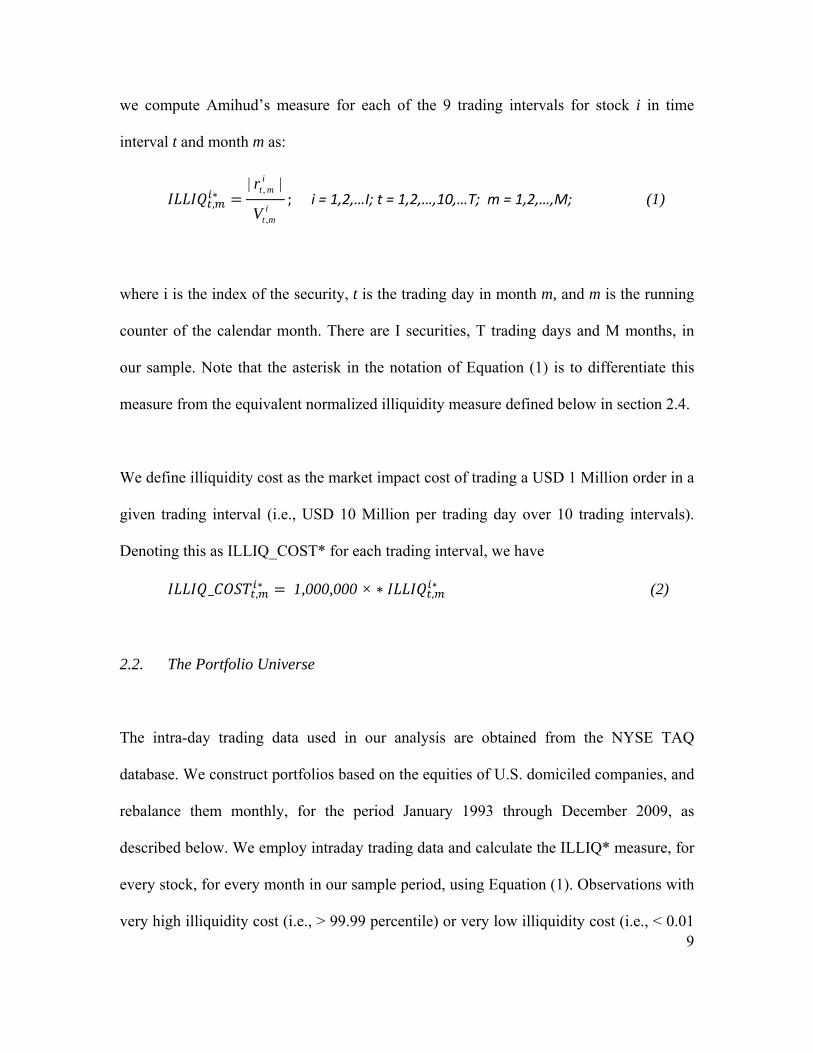
we compute Amihud’s measure for each of the 9 trading intervals for stock i in time
interval t and month m as:
,∗
|| ,i
mtr
imtV ,
; i = 1,2,…I; t = 1,2,…,10,…T; m = 1,2,…,M; (1)
where i is the index of the security, t is the trading day in month m, and m is the running
counter of the calendar month. There are I securities, T trading days and M months, in
our sample. Note that the asterisk in the notation of Equation (1) is to differentiate this
measure from the equivalent normalized illiquidity measure defined below in section 2.4.
We define illiquidity cost as the market impact cost of trading a USD 1 Million order in a
given trading interval (i.e., USD 10 Million per trading day over 10 trading intervals).
Denoting this as ILLIQ_COST* for each trading interval, we have
_ ,∗ 1,000,000 × ∗ ,
∗ (2)
2.2. The Portfolio Universe
The intra-day trading data used in our analysis are obtained from the NYSE TAQ
database. We construct portfolios based on the equities of U.S. domiciled companies, and
rebalance them monthly, for the period January 1993 through December 2009, as
described below. We employ intraday trading data and calculate the ILLIQ* measure, for
every stock, for every month in our sample period, using Equation (1). Observations with
very high illiquidity cost (i.e., > 99.99 percentile) or very low illiquidity cost (i.e., < 0.01
10
percentile) are dropped. At the end of each month, we sort stocks (for which ILLIQ* data
are available) by average market capitalization for the month, and then construct an
equally-weighted portfolio of the largest 3,000 stocks. We maintain this portfolio
constant for the following month, and repeat the process at the end of each month. This
monthly-rebalanced, equally-weighted portfolio is used for the empirical analysis in this
paper.
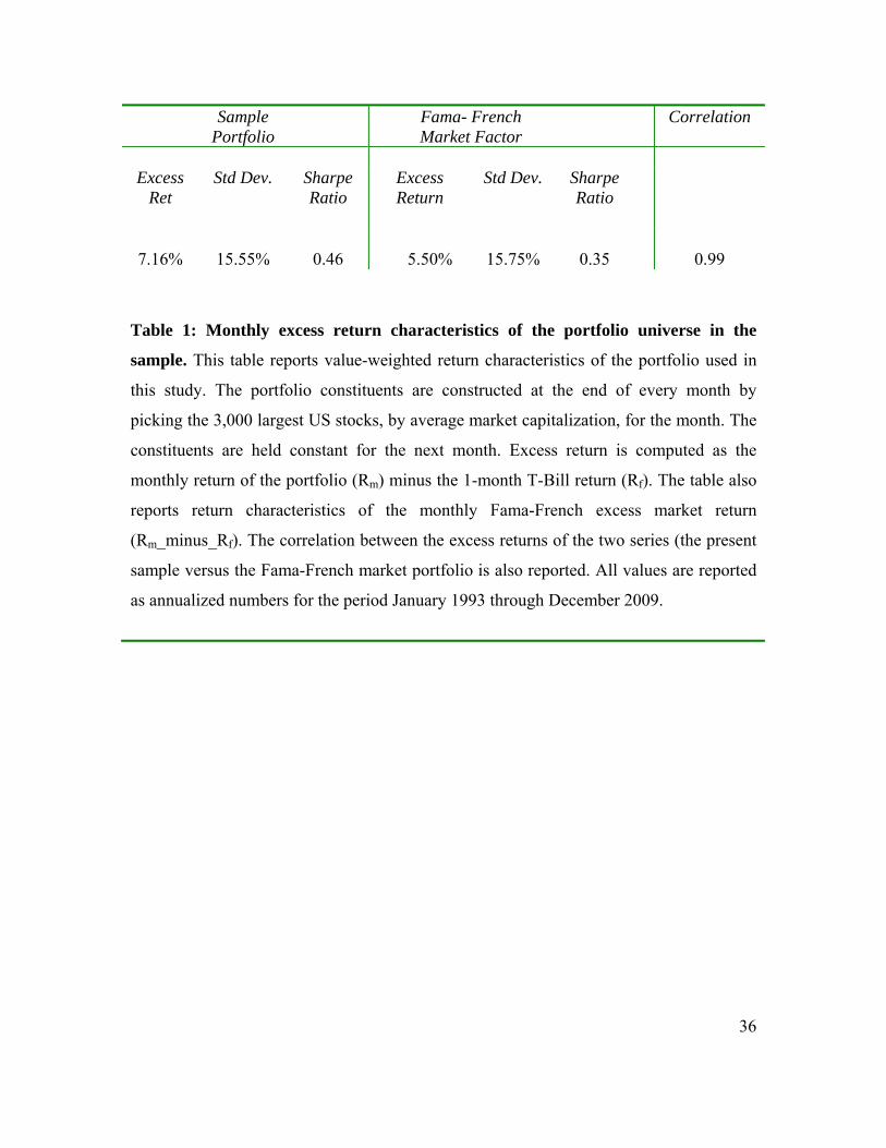
Table 1 provides a summary of the excess return characteristics of this portfolio universe,
and compares it with the return characteristics of the Fama-French market excess return
factor (market return minus the risk-free interest rate).5 In order to make an unbiased
comparison with the Fama-French market factors, the value-weighted return
characteristics of the portfolio universe are calculated. This table reports that the monthly
return correlation between our sample and that of Fama-French is over 99%, indicating
that our portfolio sample is a good representation of the U.S. equity market. Nevertheless,
there are differences in the excess returns and Sharpe ratios between the two. This is due
to the fact that the Fama-French market factor portfolio is an annually rebalanced, value-
weighted portfolio, whereas the value-weighted portfolio universe constructed here is
based on monthly rebalancing.
<Insert Table 1 Here>
2.3. Descriptive Statistics
5 See Fama and French (1992) and (1993).
11
We next present descriptive statistics of ILLIQ* formed portfolios using the universe
described above. We form five portfolios, 1 through 5, sorted using the monthly average
of ILLIQ*. Portfolio 1 is the most liquid (i.e., lowest ILLIQ*), while Portfolio 5 is the
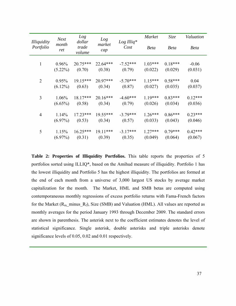
most illiquid (i.e., highest ILLIQ*). Table 2 indicates that the monthly illiquidity
premium for U.S. equities is 19 basis points. The illiquidity premium is defined as the
difference between the return to illiquid stocks (Portfolio 5) and the return to liquid
stocks (Portfolio 1). The corresponding liquidity cost differential is 413 basis points, as
measured by ILLIQ_COST*, indicating that the average holding period necessary to
realize the positive illiquid premium is around 22 months.
Table 2 also compares ILLIQ* with other proxies for illiquidity, such as the dollar
trading volume and market capitalization for each of the five portfolios based on monthly
rebalancing. The dollar trading volume and market capitalization of illiquid stocks
(Portfolio 5) is 1/90th and 1/34th of liquid stocks (Portfolio 1), respectively. Table 2 also
indicates that liquid stocks have lower market, size and valuation betas as compared to
illiquid stocks. The betas are computed using contemporaneous regressions of portfolio
excess returns of the monthly Fama-French factors as the exogenous variables. Portfolio
1 has a low beta to the size factor, which is a commonly used proxy for liquidity.
Moreover, it has an insignificant beta against the valuation factor. The results are similar
to, but somewhat stronger than, those obtained using yearly rebalancing by Fama and
French (1992).
<Insert Table 2 here>
12
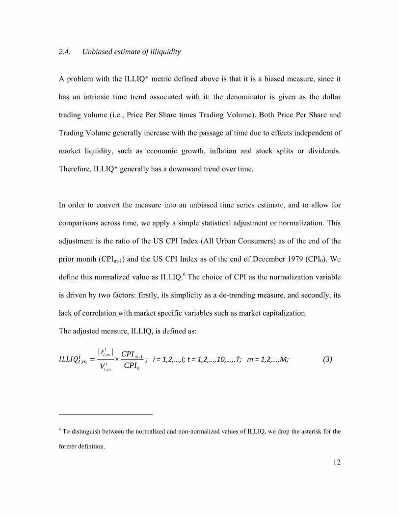
2.4. Unbiased estimate of illiquidity
A problem with the ILLIQ* metric defined above is that it is a biased measure, since it
has an intrinsic time trend associated with it: the denominator is given as the dollar
trading volume (i.e., Price Per Share times Trading Volume). Both Price Per Share and
Trading Volume generally increase with the passage of time due to effects independent of
market liquidity, such as economic growth, inflation and stock splits or dividends.
Therefore, ILLIQ* generally has a downward trend over time.
In order to convert the measure into an unbiased time series estimate, and to allow for
comparisons across time, we apply a simple statistical adjustment or normalization. This
adjustment is the ratio of the US CPI Index (All Urban Consumers) as of the end of the
prior month (CPIm-1) and the US CPI Index as of the end of December 1979 (CPI0). We
define this normalized value as ILLIQ.6 The choice of CPI as the normalization variable
is driven by two factors: firstly, its simplicity as a de-trending measure, and secondly, its
lack of correlation with market specific variables such as market capitalization.
The adjusted measure, ILLIQ, is defined as:
, || ,
imtr
imtV ,
×0
1
CPI
CPIm ; i = 1,2,…,I; t = 1,2,…,10,…,,T; m = 1,2,…,M; (3)
6 To distinguish between the normalized and non-normalized values of ILLIQ, we drop the asterisk for the
former definition.
13
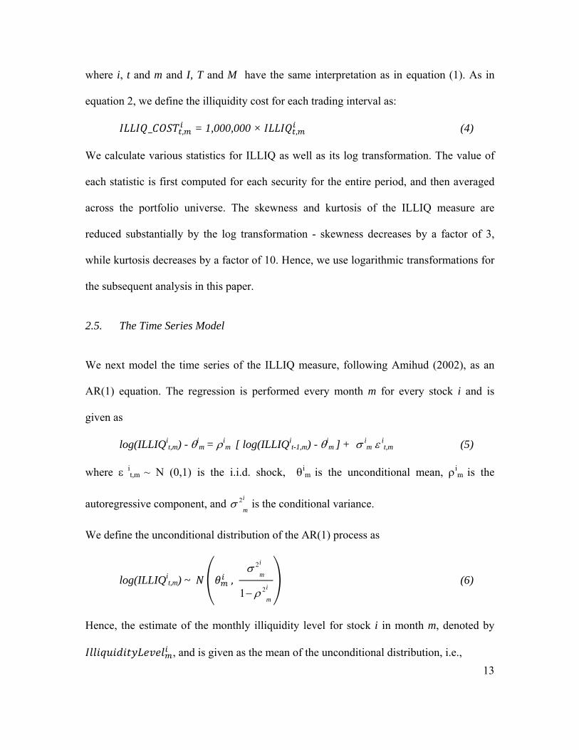
where i, t and m and I, T and M have the same interpretation as in equation (1). As in
equation 2, we define the illiquidity cost for each trading interval as:
_ , = 1,000,000 × , (4)
We calculate various statistics for ILLIQ as well as its log transformation. The value of
each statistic is first computed for each security for the entire period, and then averaged
across the portfolio universe. The skewness and kurtosis of the ILLIQ measure are
reduced substantially by the log transformation - skewness decreases by a factor of 3,
while kurtosis decreases by a factor of 10. Hence, we use logarithmic transformations for
the subsequent analysis in this paper.
2.5. The Time Series Model
We next model the time series of the ILLIQ measure, following Amihud (2002), as an
AR(1) equation. The regression is performed every month m for every stock i and is
given as
log(ILLIQit,m) - i
m = im [ log(ILLIQi
t-1,m) - im ] + i
m it,m (5)
where it,m ~ N (0,1) is the i.i.d. shock, i
m is the unconditional mean, im is the
autoregressive component, and i
m
2 is the conditional variance.
We define the unconditional distribution of the AR(1) process as
log(ILLIQit,m) ~ ,
i
m
2i
m
21 (6)
Hence, the estimate of the monthly illiquidity level for stock i in month m, denoted by
, and is given as the mean of the unconditional distribution, i.e.,
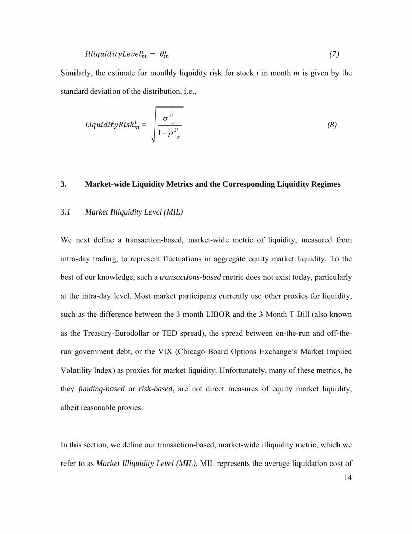
14
(7)
Similarly, the estimate for monthly liquidity risk for stock i in month m is given by the
standard deviation of the distribution, i.e.,
= i
m
i
m
2
2
1
(8)
3. Market-wide Liquidity Metrics and the Corresponding Liquidity Regimes
3.1 Market Illiquidity Level (MIL)
We next define a transaction-based, market-wide metric of liquidity, measured from
intra-day trading, to represent fluctuations in aggregate equity market liquidity. To the
best of our knowledge, such a transactions-based metric does not exist today, particularly
at the intra-day level. Most market participants currently use other proxies for liquidity,
such as the difference between the 3 month LIBOR and the 3 Month T-Bill (also known
as the Treasury-Eurodollar or TED spread), the spread between on-the-run and off-the-
run government debt, or the VIX (Chicago Board Options Exchange’s Market Implied
Volatility Index) as proxies for market liquidity. Unfortunately, many of these metrics, be
they funding-based or risk-based, are not direct measures of equity market liquidity,
albeit reasonable proxies.
In this section, we define our transaction-based, market-wide illiquidity metric, which we
refer to as Market Illiquidity Level (MIL). MIL represents the average liquidation cost of
15
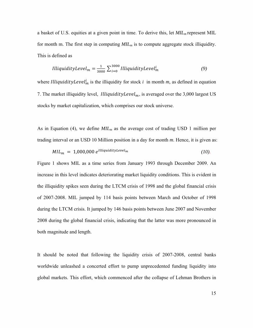
a basket of U.S. equities at a given point in time. To derive this, let MILm represent MIL
for month m. The first step in computing MILm is to compute aggregate stock illiquidity.
This is defined as
(9)
where is the illiquidity for stock i in month m, as defined in equation
7. The market illiquidity level, , is averaged over the 3,000 largest US
stocks by market capitalization, which comprises our stock universe.
As in Equation (4), we define MILm as the average cost of trading USD 1 million per
trading interval or an USD 10 Million position in a day for month m. Hence, it is given as:
1,000,000 (10).
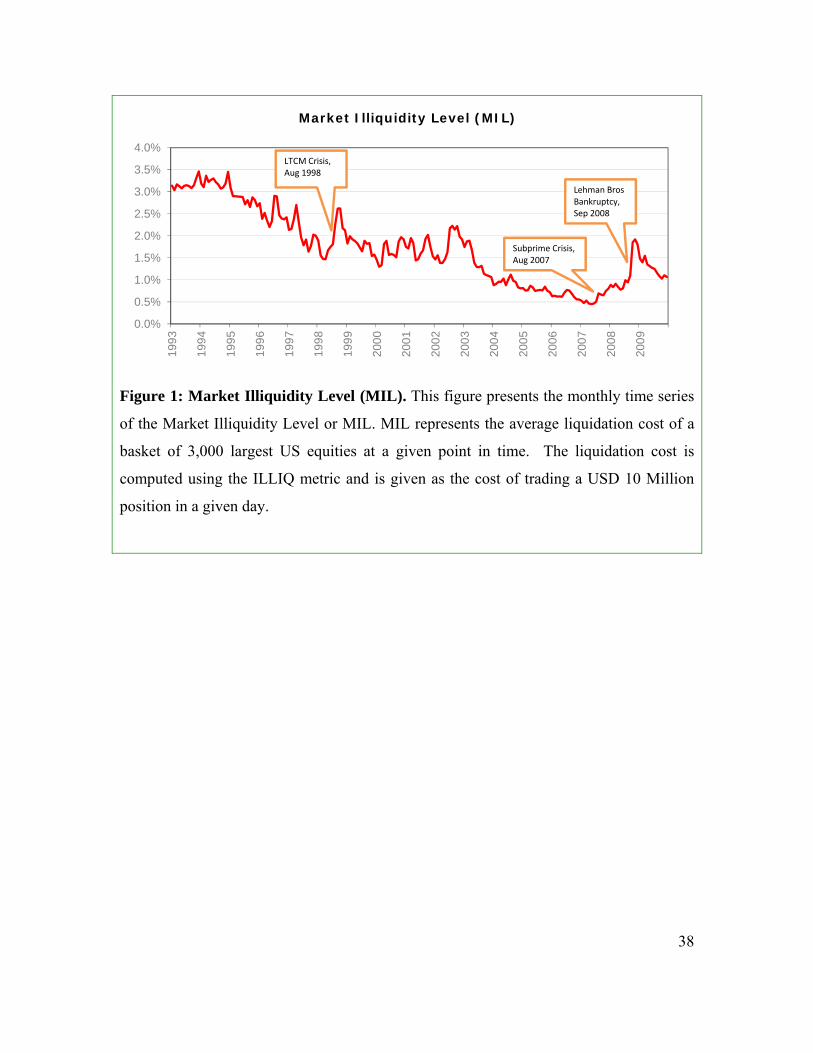
Figure 1 shows MIL as a time series from January 1993 through December 2009. An
increase in this level indicates deteriorating market liquidity conditions. This is evident in
the illiquidity spikes seen during the LTCM crisis of 1998 and the global financial crisis
of 2007-2008. MIL jumped by 114 basis points between March and October of 1998
during the LTCM crisis. It jumped by 146 basis points between June 2007 and November
2008 during the global financial crisis, indicating that the latter was more pronounced in
both magnitude and length.
It should be noted that following the liquidity crisis of 2007-2008, central banks
worldwide unleashed a concerted effort to pump unprecedented funding liquidity into
global markets. This effort, which commenced after the collapse of Lehman Brothers in
16
September 2008, had a substantial impact in improving market liquidity conditions, as
measured by transaction liquidity during the following year. This is evident in the decline
in MIL by 78 basis points from September 2008 through December 2009. However, as of
December 2009, liquidity conditions were still significantly worse compared to pre-crisis
levels in 2007.
< Insert Figure 1 here >
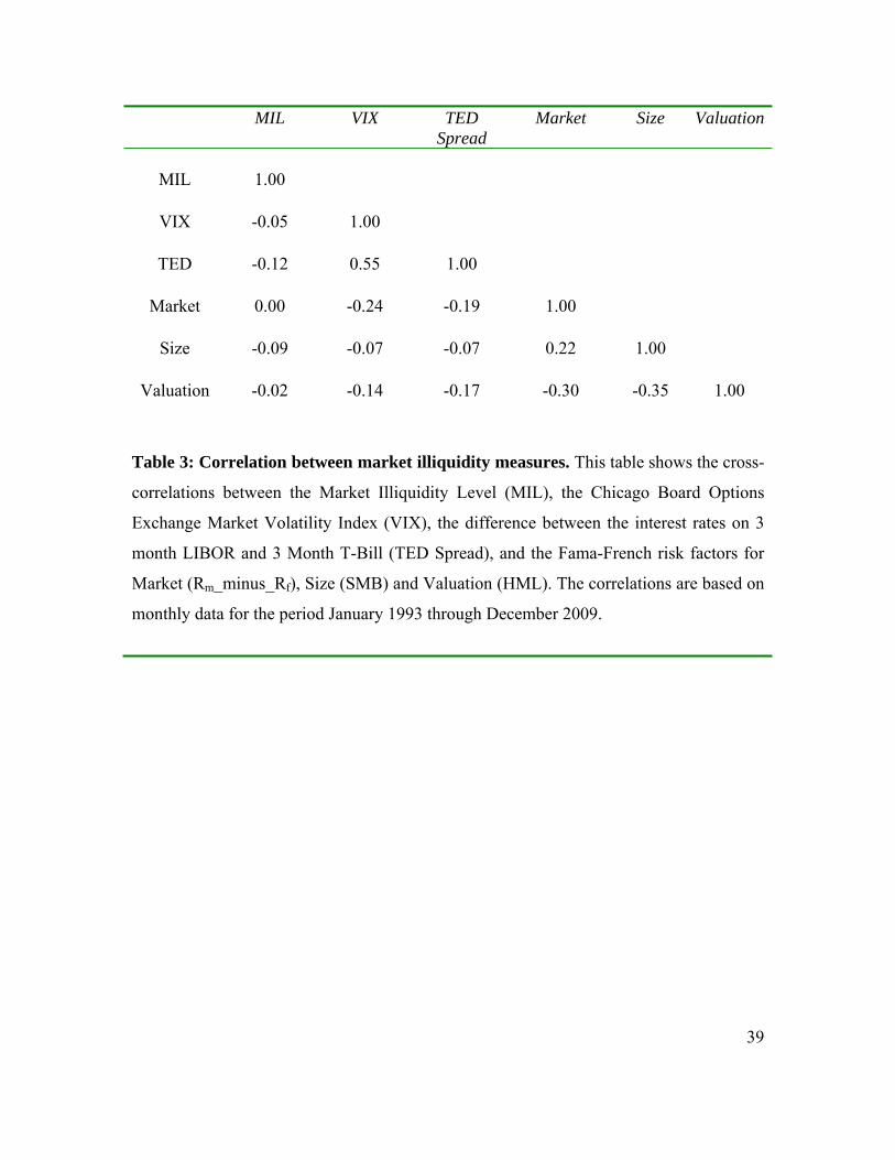
Table 3 reports the coefficients of correlation between MIL and other commonly-used
proxies for illiquidity and the Fama-French risk factors. The liquidity proxies used are the
VIX and the TED spread. As observed in the table, the degree of correlation between
MIL and the other liquidity proxies, including the SMB factor, is small. One of the
reasons why MIL is weakly correlated to the SMB factor may be because the pricing of
illiquidity often lags the actual state of illiquidity in the market. Additionally, the SMB
factor, while capturing the size premium, does not capture the true illiquidity premium,
which may also exist for some stocks with large market capitalization, albeit to a lesser
extent as compared to smaller stocks. Furthermore, as discussed in Section 3.3 below,
during periods of extreme market illiquidity, liquid stocks may actually underperform
illiquid stocks, as the former are easier to offload in order to meet de-leveraging targets
and broker margin calls.
In summary, Table 3 suggests that MIL measures an entirely different aspect of liquidity
in the market as a whole.
< Insert Table 3 here >
17
3.2 Market Illiquidity Factor (MIF)
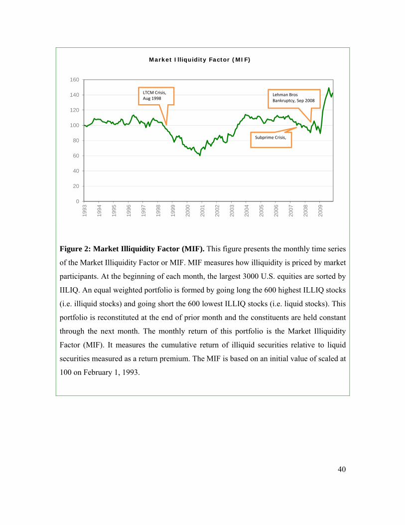
We next introduce an index to measure how illiquidity is priced by market participants,
which we call the Market Illiquidity Factor (MIF). It is computed on a monthly basis as
follows. At the beginning of each month, the largest 3000 U.S. equities (as defined in
Section 2.2) are sorted by the prior month’s illiquidity as defined in Equation 7. An
equally-weighted portfolio is formed by going long the 600 most illiquid stocks (i.e., the
top quintile) and going short the 600 least illiquid stocks (i.e., the bottom quintile). The
constituents of the portfolio are held constant for the remainder of the month, while the
portfolio is rebalanced at the beginning of each month. The monthly return of this
portfolio, which is the Market Illiquidity Factor (MIF), is shown in Figure 2. It measures
the cumulative return of illiquid securities relative to liquid securities, and can be thought
of as the market price of illiquidity measured as a return premium. The MIF for U.S.
equities is based on an initial value of 100 registered on February 1, 1993.
< Insert Figure 2 here >
Table 4 reports the monthly correlations between the MIF and the Fama-French risk
factors – namely market, size and valuation. The correlations are performed using
monthly data for the period February 1993 - December 2009.
< Insert Table 4 here >
18
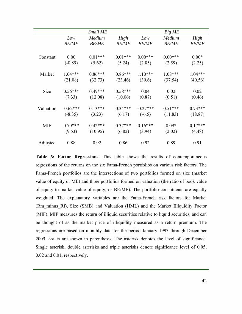
Discuss this more clearly. In Table 5, we report factor regressions of the six Fama-
French portfolios based on size and value. The regressions are performed using monthly
data for the period 1994 - 2009. The portfolios, which are constructed at the end of June
each year, are the intersection of two portfolios formed on size (market value of equity,
ME) and three portfolios formed on the ratio of book value of equity to market value of
equity (BE/ME). The size breakpoint for year t is the NYSE median market value of
equity at the end of June of year t. The BE/ME ratio of year t is the book value of equity
for the previous fiscal year end in t-1 divided by the market value of equity at the end of
December of year t-1. The BE/ME break-points are the NYSE’s 30th and 70th percentiles.
The portfolio returns are based on equally-weighted constituents. The explanatory
variables are the Fama-French risk factors (Market: Rm_minus_Rf ; Size: SMB ; and
Valuation: HML) and the Market Illiquidity Factor (MIF).
It is interesting to note from Table 5 that MIF is a significant factor in the presence of the
commonly-used factors in asset pricing tests. In the absence of any explicit market
illiquidity factor such as MIF, the SMB factor is a commonly-used proxy for liquidity in
various asset pricing regressions. In the presence of MIF, the SMB factor is rendered
insignificant for large capitalization (Big ME) portfolios. As expected, MIF loadings for
large capitalization portfolios are smaller than the loadings for small capitalization
portfolios.
3.3 Determining Market Liquidity Regimes using MIL and MIF

19
The state of liquidity in a market has two dimensions – the level of illiquidity, as
measured by MIL, and the pricing of illiquidity by market participants, as measured by
MIF. Hence, our approach to modeling liquidity herein is rich enough to allow us to
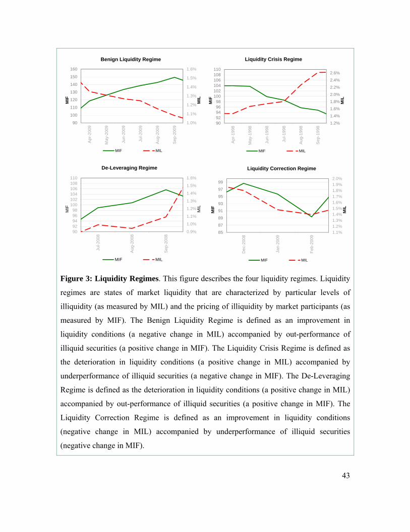
describe four distinct states of market liquidity, or liquidity regimes.
1. Benign Liquidity Regime: This state is defined as an improvement in liquidity
conditions (negative change in the MIL) accompanied by an out-performance of
illiquid securities (positive change in the MIF). As an example, the year 2009
witnessed a sharp improvement in liquidity conditions as a consequence of the
concerted effort by central banks to flush markets with liquidity. Markets
responded by pricing illiquidity favorably, leading to an increase in the MIF.
< Insert Table 5 here >
2. Liquidity Crisis Regime: This state is defined as the deterioration in liquidity
conditions (positive change in the MIL) accompanied by underperformance of
illiquid securities (negative change in the MIF). The LTCM liquidity crisis of
1998 is a case in point.
3. De-Leveraging Regime: This state is defined as the deterioration in liquidity
conditions (positive change in the MIL) accompanied by out-performance of
illiquid securities (positive change in the MIF). This pattern typically lasts for
short periods of time. It occurs during periods of extreme market stress such as in
June 2008 through September 2008, when market participants were forced to shed
positions quickly to raise capital. As the most liquid securities are easiest to
liquidate, they bear the brunt of the selling pressure, and hence the most
deterioration in price relative to illiquid securities, thereby pushing up the MIF.
20
4. Liquidity Correction Regime: This state is defined as an improvement in liquidity
conditions (negative change in the MIL) accompanied by an underperformance of
illiquid securities (negative change in the MIF). This pattern also lasts for short
periods of time. It typically occurs after a de-leveraging regime, when market
participants correct for the dislocation in security markets by dumping illiquid
securities, which were difficult to sell during the prior period of severe market
stress.
< Insert Figure 3 here>
4. Illiquidity and Asset Pricing
Traditional equilibrium asset pricing models are based on the assumption of standard,
perfectly competitive, Walrasian markets that are frictionless. However, in reality,
markets are plagued by various forms of frictions such as illiquidity and transaction costs.
Hence, prices are not always at fundamental value, and are affected by trading activity.
As a consequence, asset pricing models should incorporate liquidity as an endogenous
factor, as argued by Amihud (2002). However, one should first establish that this factor
is indeed priced in the cross-section of asset returns.
Our goal in this section is to test whether the illiquidity measures derived in Section 2,
have incremental explanatory power for the cross-section of asset returns relative to the
Fama-French 3-factor model. First, for each month, we sort our universe of 3,000 stocks
by the stock Illiquidity Level as defined in Section 2.5, in ascending order, and split them
into 100 portfolios with 30 stocks in each portfolio. We obtain rolling estimates of Fama
21
and French factor loadings for each portfolio p and each month m, by using a regression
of the past 60 months of excess return data. The regression equation is given as
(11)
Where is the portfolio return computed as an equally-weighted average return of
the constituents, and is the risk free rate, , and are the factor
loadings for the Fama and French factors (Market), (Size) and
(Valuation) respectively and is the error term.
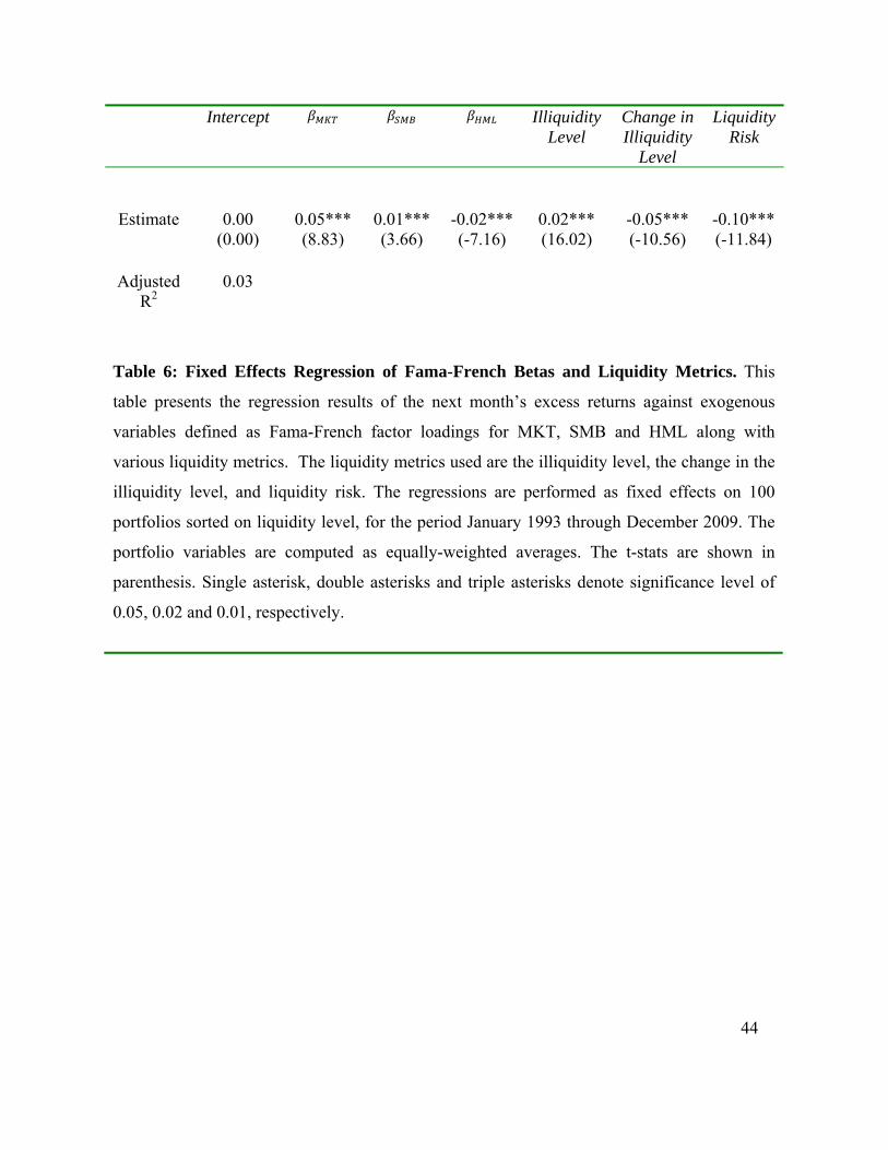
Next, we seek to explain the next period’s excess return with the exogenous variables
given as the Fama-French factor loadings computed as above, along with the illiquidity
level, liquidity risk and change in illiquidity level for the portfolio. The illiquidity level
and liquidity risk of the portfolio are computed as equally-weighted averages of the
constituents. We denote them by and respectively
for portfolio p in month m.
The change in the illiquidity level of portfolio p between month m-1 and m is given as
= (12)
The fixed-effects regression equation can then be formulated as
(13)

22
where ( represents the time invariant intercept for every portfolio p and
, , , , and are the regression
coefficients.7 Under the null hypothesis, ( should only depend on
, , and . As a consequence, the loadings for Illiquidity, i.e.,
. and should be 0, under the null hypothesis
that only the Fama-French factors are priced.
Table 6, however, demonstrates that all three coefficients of the liquidity factors are
statistically significant. Hence, we can reject the null hypothesis and establish that the
level of illiquidity, the change in the illiquidity from the prior period, and liquidity risk
are important in explaining future asset returns. The positive loading for the illiquidity
level is to be expected as market participants need to be compensated for the higher
transaction cost of owning illiquid securities.
However, the negative loadings for changes in the illiquidity level and liquidity risk
(which both measure the volatility in liquidity) contradict traditional wisdom. A negative
correlation is also observed in Chordia, Subrahmanyam and Anshuman (2001), O’Hara
(2002), Chollete (2004), and Fu (2008). Chen (2008) explains this phenomenon as the
volatility of liquidity being driven by the idiosyncratic risk of the stock that cannot be
7 We are not directly interested in the estimation of the fixed effects, i.e. . The fixed effects are removed
by time de-meaning each variable (the so called within estimator), i.e. ,
etc.
23
diversified away.. Conventional wisdom indicates that if investors are not able to fully
diversify risk, then they will demand a premium for holding stocks with high
idiosyncratic risk. Merton (1987) suggests a rationale for this phenomenon in an
information-segmented market, in which firms with larger firm-specific variances require
higher returns to compensate investors for holding imperfectly diversified portfolios.
Therefore, the negative premium observed in this study and other papers in the literature
may be related to as the idiosyncratic risk premium puzzle.
< Insert Table 6 here>
5. A Simple Liquidity-based Trading Strategy
5.1 Does liquidity in the prior period influences the returns in the subsequent period?
If illiquidity is indeed being awarded a return premium, it would be interesting to
examine whether an investment trading strategy can be established to exploit the
illiquidity premium by trading illiquid assets against their liquid counterparts, after
adjusting for risk. To analyze this, we first examine whether a liquidity trading strategy,
which sorts equally-weighted portfolios of the largest 3,000 stocks by illiquidity quintiles
using ILLIQ* (see Section 2.2), can produce excess returns. This is similar in spirit to
other trading strategies reported in the academic literature involving portfolio quintiles or
deciles.
We next study this issue from a practical perspective by examining whether a similar
liquidity trading strategy involving actively traded stock market indices, which differ
24
substantially in terms of the liquidity of their component stocks, can also produce
significant returns.
For the trading strategy using illiquid and liquid securities, we define the benchmark
portfolio as being long the most illiquid quintile portfolio and short the most liquid
quintile portfolio, over the entire sample period. We maintain this static benchmark
portfolio throughout the trading period. Similarly for the trading strategy based on stock
market indices, we define the benchmark as being long the Russell 2000 index (a stock
index proxy for illiquid securities) and short the Dow Jones Industrial Average (a stock
index proxy for liquid securities).
For the purpose of calculating the trailing liquidity change for month m, we examine
MILm-1 against MILm-2, which measures the liquidity change in month m over the prior 2
months. Trailing liquidity is improving for month m, if MILm-1 < MILm-2. Similarly,
liquidity is deteriorating for month m, if MILm-1 > MILm-2.
5.2. Trading Strategy Involving Liquidity-Quintile Portfolios
Table 7 shows that equity portfolios sorted by illiquidity quintiles using ILLIQ* exhibit
superior performance when the prior liquidity improves as compared to the case when the
prior liquidity deteriorates. More specifically, we construct two liquidity-sorted portfolios
based on the prior month's ILLIQ score - a low liquidity portfolio consisting of the top
ILLIQ quintile stocks, and a high liquidity portfolio consisting of the bottom ILLIQ
quintile stocks.
25
For example, when liquidity deteriorates, the most liquid portfolio almost always has a
higher return on average than the most illiquid portfolio. This outcome generally reverses
when market liquidity conditions improve. Furthermore, both the most liquid and most
illiquid portfolios have higher volatility in markets with deteriorating liquidity, as
compared to their respective volatility when liquidity is improving.
< Insert Table 7 here >
The empirical evidence here demonstrates that illiquid stocks, on average, outperform
liquid stocks when liquidity improves, and vice versa. This would suggest a trading
strategy involving buying the illiquid stocks (or index) when liquidity conditions are
improving. Similarly when liquidity conditions are deteriorating, it calls for buying the
liquid stocks (or index). This central finding governs the implementation of our trading
strategy as described in the section below. We do this by using the most liquid and
illiquid portfolios, by quintiles, for both monthly and weekly rebalancing, albeit by using
the same monthly change in liquidity in both cases, i.e., by comparing MILm-1 against
MILm-2.
As discussed above, we first implement a naïve investment trading strategy that takes a
long position in the most illiquid quintile portfolio when prior liquidity is improving.
Conversely, the strategy takes a long position in the most liquid quintile portfolio when
prior liquidity is deteriorating. The most liquid and most illiquid portfolios are
constructed based on the liquidity quintiles approach described heretofore. This strategy
does not take into account transaction costs, and is rebalanced on a monthly as well as
weekly basis.
26
Our liquidity model is based on a partial equilibrium model of intraday trading, where the
liquidity signal changes rapidly as new price and volume information arrive and get
incorporated on a high frequency basis. The more frequent the revision in the trading
strategy in response to a signal, the smaller the time-decay in the trading signal’s efficacy.
As a consequence, we conducted the trading strategy over two different rebalancing
cycles, mainly weekly and monthly.
While the empirical analysis and tests in the paper have been based on monthly
rebalancing up until now, we introduce weekly rebalancing in this trading strategy
section, purely to take advantage of the illiquidity signal’s changing strength as new
information is incorporated into the signal’s parameters. Weekly rebalancing would also
take into account the realities of active portfolio trading, which would require more
frequent revisions of the portfolio, due to corresponding revisions in the signal.
Figures 4a and 4b demonstrate that the dynamic liquidity-sorted portfolio trading strategy
for the trading period March 1993 through December 2009 strongly outperforms a naïve
benchmark. As defined above, the static benchmark is long the most illiquid quintile
portfolio and short the most liquid quintile portfolio, held over the entire sample period.
< Insert Figure 4a here >
< Insert Figure 4b here >
The dark colored line in each graph represents the performance of the static benchmark
portfolio, while the light colored line represents the performance of the dynamic
liquidity-sorted portfolio strategy. As is evident, the dynamic strategy clearly
27
outperforms the static benchmark strategy. The extent of the outperformance is greater
for the weekly rebalancing (in Figure 4b) than for the monthly rebalancing (in Figure 4a),
demonstrating the importance of a timely response to the signal. The trading strategy
performance is quite robust across various liquidity cycles.
We next conduct a factor regression of the liquidity-based trading strategies for both
monthly and weekly rebalancing frequencies. Table 9 provides the results of the
contemporaneous regression of monthly returns of liquidity based on monthly and
weekly rebalanced long/short trading strategies. The exogenous variables are the Fama-
French risk factors for market, size (SMB) and valuation (HML). The regression is
estimated based on the two liquidity-sorted portfolios. The strategies take a long position
in the low liquidity portfolio and a short position in the high liquidity portfolio when
prior liquidity is improving. Conversely, the strategies take a short position in the low
liquidity portfolio and a long position in the high liquidity portfolio when prior liquidity
is deteriorating. Liquidity is improving when the Market Illiquidity Level (MIL)
decreases over the prior 2 months, and irrespective of the rebalancing frequency.
Liquidity is deteriorating when the MIL increases over the prior 2 months, again
irrespective of the rebalancing frequency.
As Table 8 indicates, the Sharpe ratio for the liquidity-based trading strategy is much
stronger when the portfolio is rebalanced on a weekly basis versus when it is rebalanced
on a monthly basis. The liquidity-based trading strategy yields an annualized Sharpe ratio
and alpha of 0.72 and 9.63%, respectively, for the weekly rebalanced liquidity-based
portfolio strategy, versus 0.29 and 4.18% for the monthly rebalanced one.
28
< Insert Table 8 here >
We observe from the above table that a weekly rebalanced liquidity-based portfolio has
much better risk-adjusted performance as compared to the monthly rebalanced one, as
also seen in Figures 4a and 4b.
The above discussion also reflects a common phenomenon in quantitatively-driven
portfolio trading strategies, where the portfolio backtests are carried out on a monthly
frequency and over a much longer data test period, whereas the strategy itself is deployed
as a live portfolio with more active rebalancing so as to mitigate the signal’s time decay
effect. The implicit assumption made herein is that the model of equilibrium presented is
invariant to the rebalancing frequency, which would be a function of signal turnover,
transaction costs, data availability, and so on.
5.3. Trading Strategy Involving Index Portfolios
Since an argument can be made that it would be too costly to transact the liquidity-based
trading strategy based on illiquidity quintiles, we provide here a simple index-level
trading strategy, which would have much lower transaction costs. For this index-level
liquidity trading strategy, we analyze the return distribution of U.S. equity indices when
the trailing liquidity, as measured by the Market Illiquidity Level (MIL), is improving
versus when the trailing liquidity is deteriorating. For the purpose of implementing an
investment trading strategy with relatively low transaction costs, we consider two
different U.S. equity indices with component stocks exhibiting different liquidity
characteristics. Both the indices exist as very liquid Exchange Traded Funds (ETFs), or
as futures contracts, and hence can be traded as a basket with minimal transaction costs.
29
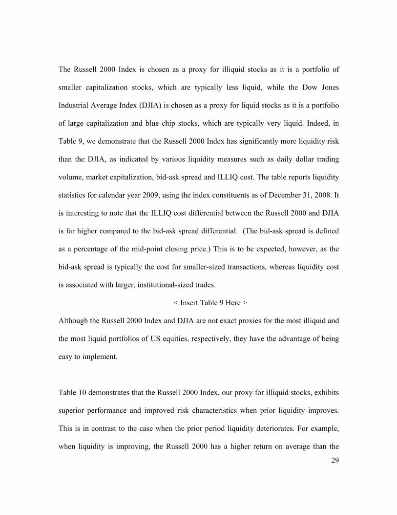
The Russell 2000 Index is chosen as a proxy for illiquid stocks as it is a portfolio of
smaller capitalization stocks, which are typically less liquid, while the Dow Jones
Industrial Average Index (DJIA) is chosen as a proxy for liquid stocks as it is a portfolio
of large capitalization and blue chip stocks, which are typically very liquid. Indeed, in
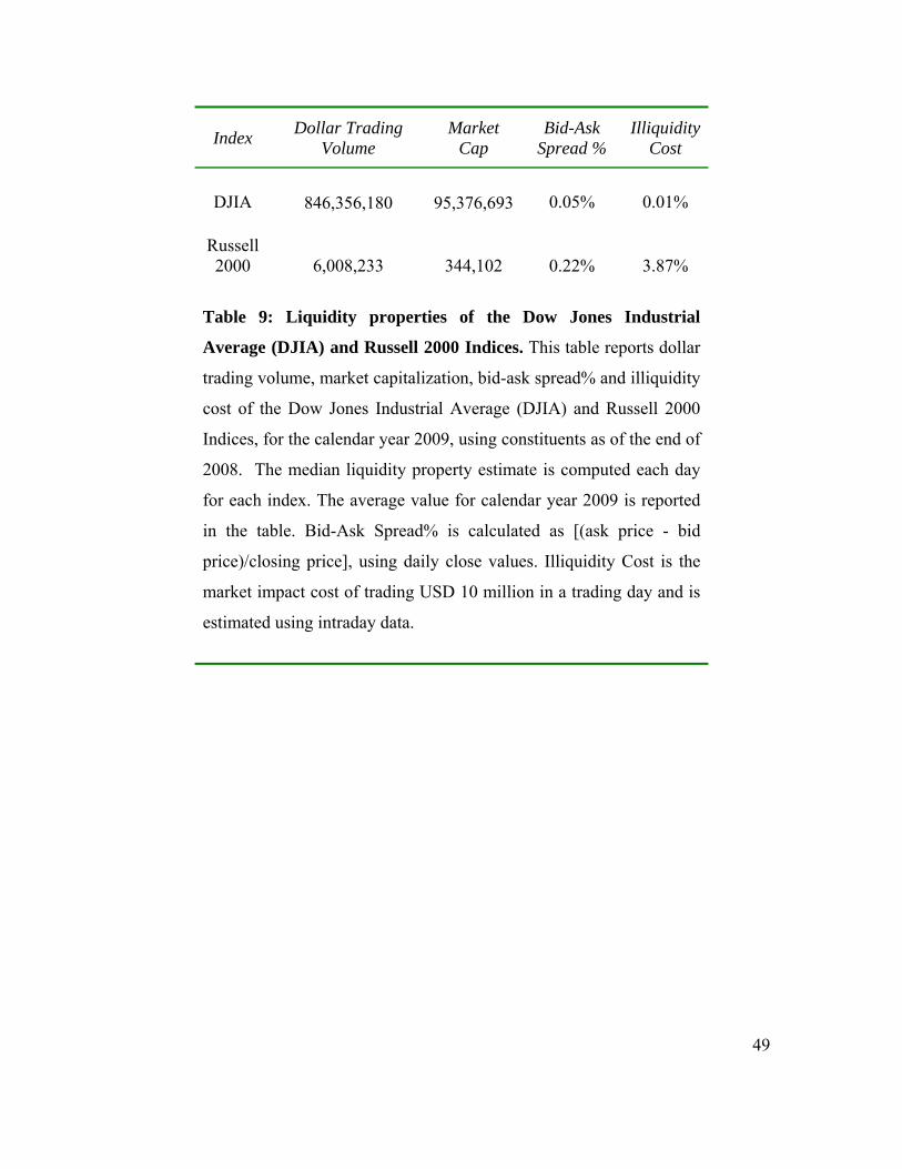
Table 9, we demonstrate that the Russell 2000 Index has significantly more liquidity risk
than the DJIA, as indicated by various liquidity measures such as daily dollar trading
volume, market capitalization, bid-ask spread and ILLIQ cost. The table reports liquidity
statistics for calendar year 2009, using the index constituents as of December 31, 2008. It
is interesting to note that the ILLIQ cost differential between the Russell 2000 and DJIA
is far higher compared to the bid-ask spread differential. (The bid-ask spread is defined
as a percentage of the mid-point closing price.) This is to be expected, however, as the
bid-ask spread is typically the cost for smaller-sized transactions, whereas liquidity cost
is associated with larger, institutional-sized trades.
< Insert Table 9 Here >
Although the Russell 2000 Index and DJIA are not exact proxies for the most illiquid and
the most liquid portfolios of US equities, respectively, they have the advantage of being
easy to implement.
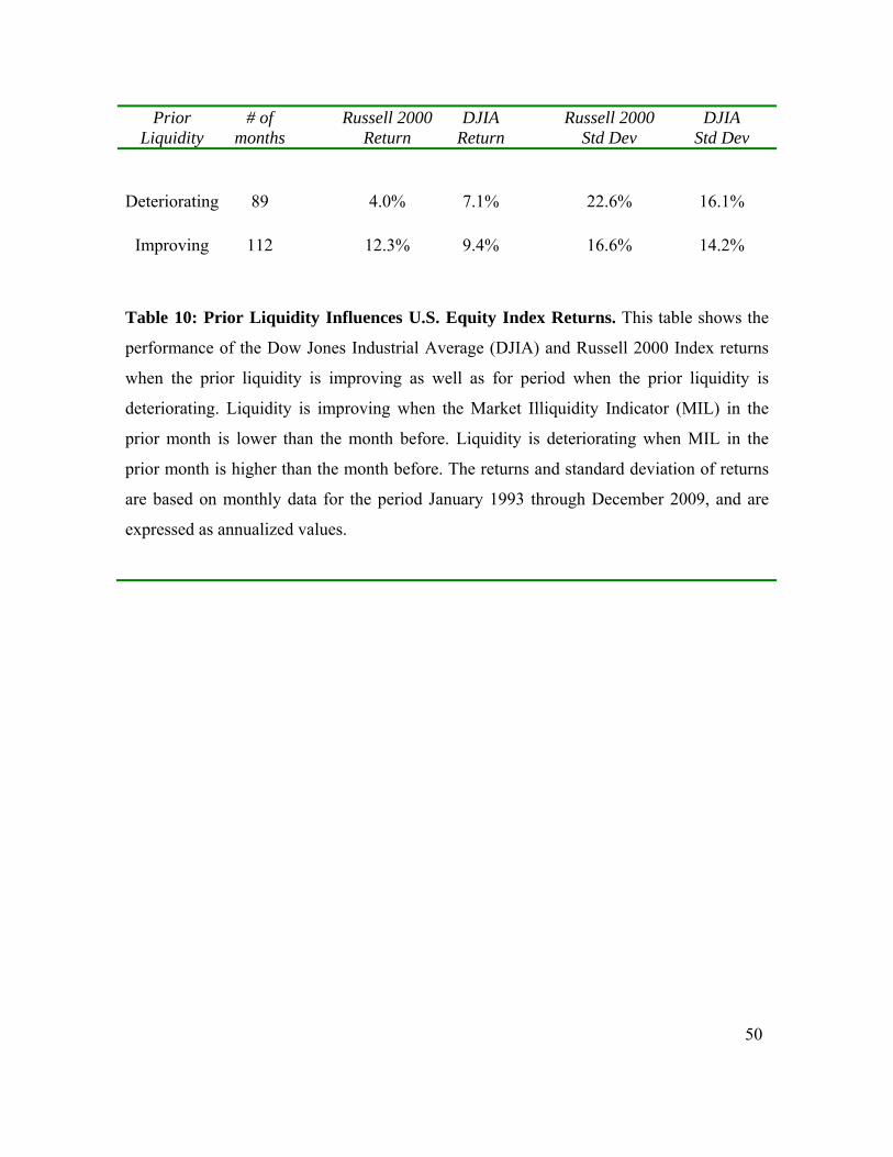
Table 10 demonstrates that the Russell 2000 Index, our proxy for illiquid stocks, exhibits
superior performance and improved risk characteristics when prior liquidity improves.
This is in contrast to the case when the prior period liquidity deteriorates. For example,
when liquidity is improving, the Russell 2000 has a higher return on average than the
30
DJIA, which is our proxy for liquid stocks. This outcome reverses during deteriorating
conditions of market liquidity. Furthermore, both the DJIA and Russell 2000 have lower
volatility in markets with improving liquidity, as compared to their respective volatility
when liquidity is deteriorating.
< Insert Table 10 here >
As we did in the previous section using liquidity-sorted portfolios, we next implement a
naïve index-level trading strategy that takes a long position in the Russell 2000 Index and
a short position in the DJIA when prior liquidity is improving. Conversely, the strategy
takes a short position in the Russell 2000 and a long position in the DJIA when prior
liquidity is deteriorating. Again, the strategy does not take into account transaction costs.
However, the analysis is once again conducted and reported on both a monthly and
weekly rebalancing basis.
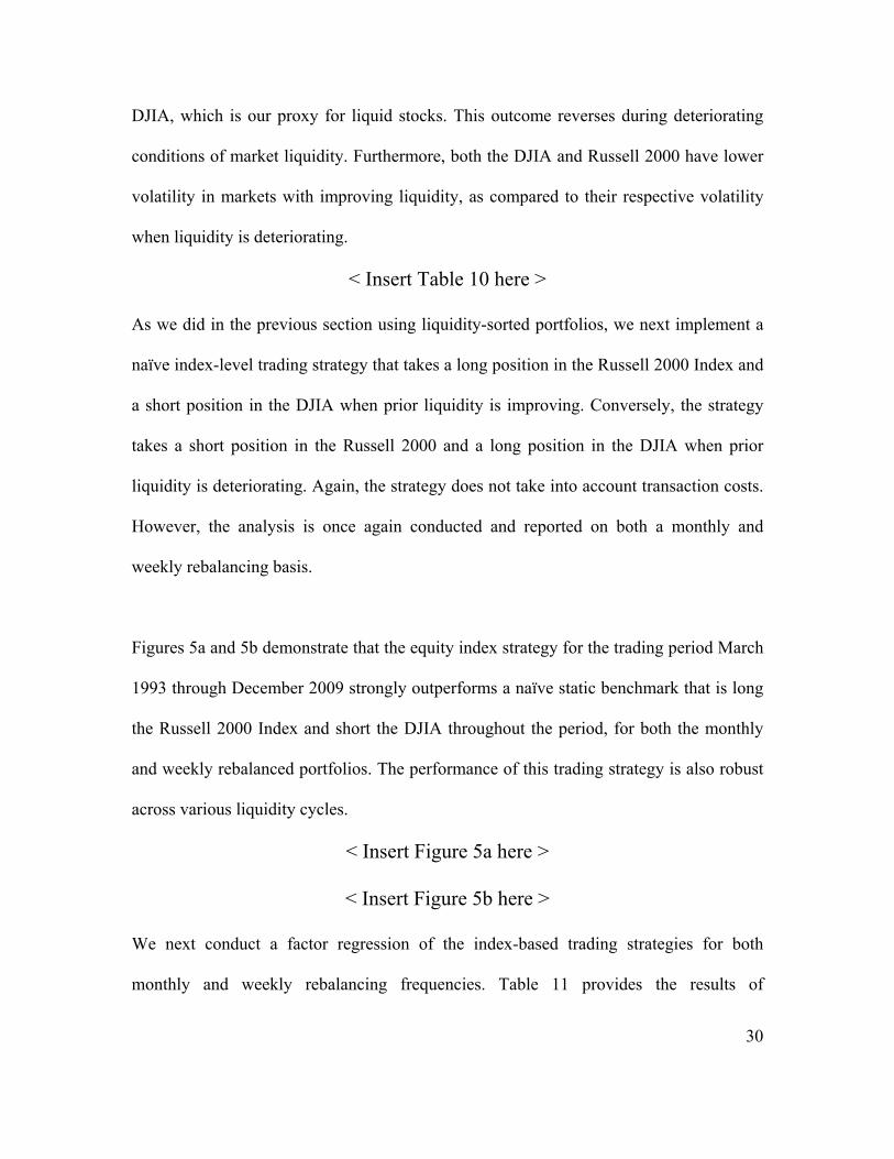
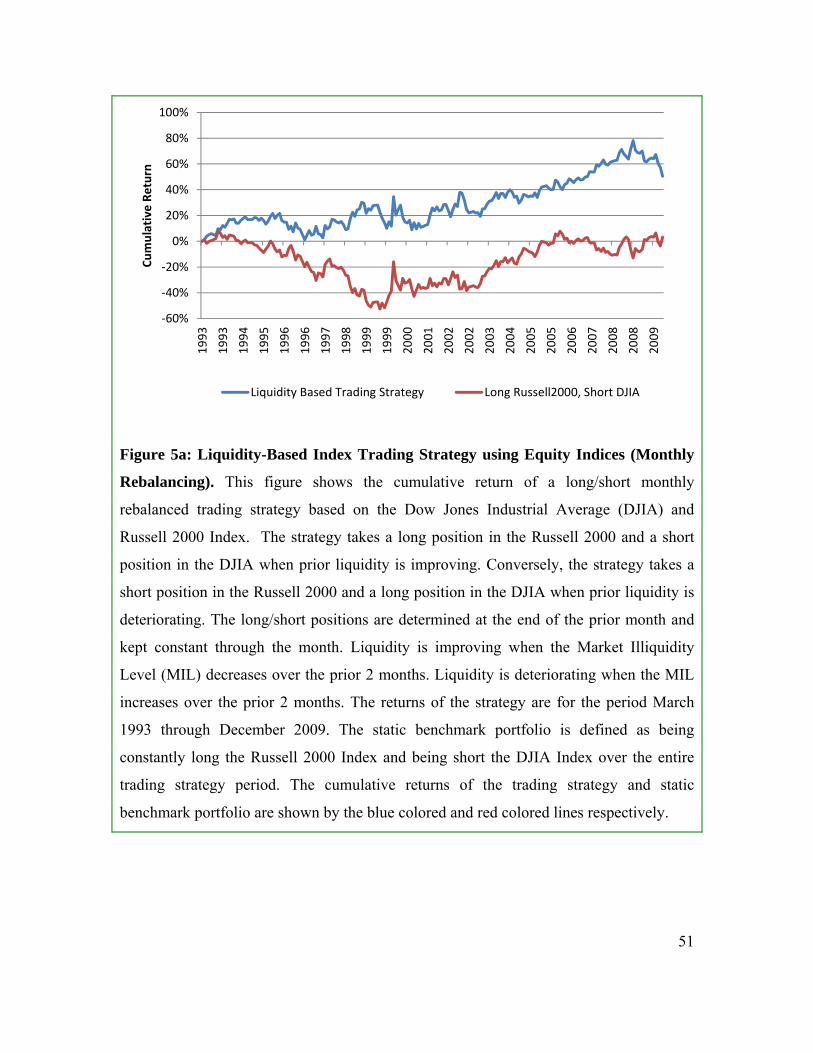
Figures 5a and 5b demonstrate that the equity index strategy for the trading period March
1993 through December 2009 strongly outperforms a naïve static benchmark that is long
the Russell 2000 Index and short the DJIA throughout the period, for both the monthly
and weekly rebalanced portfolios. The performance of this trading strategy is also robust
across various liquidity cycles.
< Insert Figure 5a here >
< Insert Figure 5b here >
We next conduct a factor regression of the index-based trading strategies for both
monthly and weekly rebalancing frequencies. Table 11 provides the results of
31
contemporaneous regressions of monthly returns of liquidity based on monthly and
weekly rebalanced long/short trading strategies. The exogenous variables are the Fama-
French risk factors for market, size (SMB) and valuation (HML). The regression is
estimated based on the Dow Jones Industrial Average (DJIA) and Russell 2000 Index.
The strategy takes a long position in the Russell 2000 Index and a short position in the
DJIA portfolio when prior liquidity is improving. Conversely, the strategy takes a short
position in the Russell 2000 and a long position in the DJIA when prior liquidity is
deteriorating. Liquidity is improving when the Market Illiquidity Level (MIL) decreases
over the prior 2 months, and irrespective of the rebalancing frequency. Liquidity is
deteriorating when the MIL increases over the prior 2 months.
As Table 11 indicates, the Sharpe ratio for the equity index trading strategy is much
stronger when the portfolio is rebalanced on a weekly basis versus when it is on a
monthly basis. The Russell 2000 Index / DJIA equity index trading strategy yields an
annualized Sharpe ratio and alpha of 0.67 and 10.02%, respectively, for the weekly
rebalanced trading strategy, versus 0.21 and 3.96% for the monthly rebalanced strategy.
These results are encouraging as, from the practical perspective, it goes to show that the
liquidity-based trading strategy described in this paper is viable and implementable as a
portfolio trading strategy, with minimal transaction costs.
< Insert Table 11 here >
32
6. Conclusion
This paper defined, developed, and empirically tested some transactions-based measures
of liquidity and liquidity risk, both at the stock- and market-levels, that are easy to
implement. By using intraday, transactions-level data to estimate the level and
uncertainty of liquidity, we provide strong empirical evidence that validates the notion
that liquidity affects financial market performance, and as a consequence, has
implications for both portfolio construction and risk management. For example, illiquid
equities ranked by our Stock Illiquidity Level indicator underperformed liquid equities by
15.8% during the 2007-2008 illliquidity build-up during the global financial crisis, and by
18.4% during the 1998 LTCM crisis.
By using new transactions-based, market-wide metrics of illiquidity, which measure the
interaction between aggregate market liquidity and the market’s pricing of liquidity risk,
we identify four different market regimes for liquidity. We also demonstrate that in the
presence of the liquidity variables introduced in this paper, commonly-used proxies for
liquidity, such as size and turnover, are rendered insignificant in explaining cross-
sectional asset returns.
Finally, as an illustration of the efficacy of our approach to understanding and exploiting
liquidity changes, two simple trading strategies were developed using the Market
Illiquidity Level indicator to generate profitable long/short investment trading strategies.
33
We first conducted a similar liquidity-based trading strategy that takes a long (short)
position in the lowest quintile liquidity portfolio and a short (long) position in the highest
quintile liquidity portfolio when prior liquidity is improving (deteriorating). The second
strategy calls for a long (short) position in the Russell 2000 Index and a short (long)
position in the Dow Jones Industrial Average Index when prior liquidity is improving
(deteriorating), The Russell 2000 Index serves as a proxy for illiquid equities, while the
Dow Jones Industrial Average Index serves as a proxy for liquid equities.
The results are fairly strong: the quintile-based, weekly rebalanced portfolio-level trading
strategy yielded an annualized return of 9.63% and a Sharpe ratio of 0.72 for the period
March 1993 through December 2009, while the corresponding index-level trading
strategy yielded an annualized return of 10.02% and a Sharpe Ratio of 0.67.
34
References
Amihud, Y., 2002. Illiquidity and stock returns: cross-section and time-series effects. Journal of Financial Markets 5, 31–56. Amihud, Y., Mendelson, H., 1986. Asset pricing and the bid-ask spread. Journal of Financial Economics 17, 223–249. Amihud, Y., Mendelson, H., 1989. The effect of beta, bid-ask spread, residual risk and size on stock returns. Journal of Finance 44, 479–486. Amihud, Y., H. Mendelson, B. Lauterbach. 1997. Market microstructure and securities values: Evidence from the Tel Aviv Exchange. Journal of Financial Economics 45, 365-390. Amihud, Y., Mendelson, H., Wood, R., 1990. Liquidity and the 1987 stock market crash. Journal of Portfolio Management, 65–69. Amihud, Y., Mendelson, H., Pedersen, L.H., 2005. Liquidity and Asset Prices. Foundations and Trends in Finance Vol. 1, No 4, 269–364. Acharya, V. V., and L. H. Pedersen. 2005. Asset Pricing with Liquidity Risk. Journal of Financial Economics 77 (2): 375–410. Brennan, M.J., Subrahmanyam, A., 1996. Market microstructure and asset pricing: on the compensation for illiquidity in stock returns. Journal of Financial Economics 41, 441–464. Brennan, M.J., Chordia, T., Subrahmanyam, A., 1998. Alternative factor specifications, security characteristics, and the cross-section of expected returns. Journal of Financial Economics 49, 345–373. Chen, Zhanhui. 2010. Volatility of Liquidity, Idiosyncratic Risk and Asset Returns. Working Paper, Texas A&M University. Chollete, Lorán. 2004. Asset pricing implications of liquidity and its volatility. Working paper, Columbia University. Chordia, T., Roll, R., Subrahmanyam, A., 2000. Commonality in liquidity. Journal of Financial Economics 56, 3–28.
35
Chordia, T., Roll, R., Subrahmanyam, A., 2001a. Market liquidity and trading activity. Journal of Finance 56, 501–530. Chordia, T., V. Anshuman, A. Subrahmanyam. 2001. Trading activity and expected stock returns. Journal of Financial Economics 59, 3-32. Fama, E.F., French, K.R., 1992. The cross-section of expected stock returns. Journal of Finance 47, 427–465. Fama, E.F., French, K.R., 1993. Common risk factors in the returns on stocks and bonds. Journal of Financial Economics 33, 3–56. Fama, E.F., MacBeth, J.D., 1973. Risk, return, and equilibrium: Empirical tests. Journal of Political Economy 81, 607–636. Hameed, A., Kang, W., Viswanathan, S., 2007. Stock Market Declines and Liquidity, NUS Working Paper..
Hasbrouck, J., Seppi, D.J., 2001. Common factors in prices, order flows and liquidity. Journal of Financial Economics 59, 383–411.
Huang, M., 2003. Liquidity shocks and equilibrium liquidity premia. Journal of Economic Theory 109, 104–129. Kyle, A.S., 1985. Continuous Auctions and Insider Trading. Econometrica Vol. 53, No. 6, 1315-1335.
Lo, A., Petrov, C., Wierzbicki., M., 2003. It’s 11 PM — Do You Know Where Your Liquidity Is? The Mean-Variance Liquidity Frontier. Journal of Investment Management.
O’Hara, M. 2003. Liquidity and price discovery. Journal of Finance 58, 1335–54. Pastor, L., Stambaugh, R.F., 2003. Liquidity risk and expected stock returns. Journal of Political Economy 111, 642–685.
36
Sample Portfolio
Fama- French Market Factor
Correlation
Excess
Ret Std Dev. Sharpe
Ratio Excess
Return Std Dev. Sharpe
Ratio
7.16% 15.55% 0.46 5.50% 15.75% 0.35 0.99
Table 1: Monthly excess return characteristics of the portfolio universe in the
sample. This table reports value-weighted return characteristics of the portfolio used in
this study. The portfolio constituents are constructed at the end of every month by
picking the 3,000 largest US stocks, by average market capitalization, for the month. The
constituents are held constant for the next month. Excess return is computed as the
monthly return of the portfolio (Rm) minus the 1-month T-Bill return (Rf). The table also
reports return characteristics of the monthly Fama-French excess market return
(Rm_minus_Rf). The correlation between the excess returns of the two series (the present
sample versus the Fama-French market portfolio is also reported. All values are reported
as annualized numbers for the period January 1993 through December 2009.
37
Illiquidity Portfolio
Next month
ret
Log dollar trade
volume
Log market
cap
Log Illiq* Cost
Market Size Valuation
Beta Beta Beta
1 0.96% 20.75*** 22.64*** -7.52*** 1.03*** 0.18*** -0.06 (5.22%) (0.70) (0.38) (0.79) (0.022) (0.029) (0.031) 2 0.95% 19.15*** 20.97*** -5.70*** 1.15*** 0.58*** 0.04 (6.12%) (0.63) (0.34) (0.87) (0.027) (0.035) (0.037) 3 1.06% 18.17*** 20.16*** -4.60*** 1.19*** 0.83*** 0.12*** (6.65%) (0.58) (0.34) (0.79) (0.026) (0.034) (0.036) 4 1.14% 17.23*** 19.55*** -3.79*** 1.26*** 0.86*** 0.23*** (6.97%) (0.53) (0.34) (0.57) (0.033) (0.043) (0.046) 5 1.15% 16.25*** 19.11*** -3.17*** 1.27*** 0.79*** 0.42*** (6.97%) (0.31) (0.39) (0.35) (0.049) (0.064) (0.067)
Table 2: Properties of Illiquidity Portfolios. This table reports the properties of 5
portfolios sorted using ILLIQ*, based on the Amihud measure of illiquidity. Portfolio 1 has
the lowest illiquidity and Portfolio 5 has the highest illiquidity. The portfolios are formed at
the end of each month from a universe of 3,000 largest US stocks by average market
capitalization for the month. The Market, HML and SMB betas are computed using
contemporaneous monthly regressions of excess portfolio returns with Fama-French factors
for the Market (Rm_minus_Rf), Size (SMB) and Valuation (HML). All values are reported as
monthly averages for the period January 1993 through December 2009. The standard errors
are shown in parenthesis. The asterisk next to the coefficient estimates denotes the level of
statistical significance. Single asterisk, double asterisks and triple asterisks denote
significance levels of 0.05, 0.02 and 0.01 respectively.
38
Figure 1: Market Illiquidity Level (MIL). This figure presents the monthly time series
of the Market Illiquidity Level or MIL. MIL represents the average liquidation cost of a
basket of 3,000 largest US equities at a given point in time. The liquidation cost is
computed using the ILLIQ metric and is given as the cost of trading a USD 10 Million
position in a given day.
0.0%
0.5%
1.0%
1.5%
2.0%
2.5%
3.0%
3.5%
4.0%
199
3
199
4
199
5
199
6
199
7
199
8
199
9
200
0
200
1
200
2
200
3
200
4
200
5
200
6
200
7
200
8
200
9
Market Illiquidity Level (MIL)
Lehman Bros Bankruptcy, Sep 2008
Subprime Crisis, Aug 2007
LTCM Crisis, Aug 1998
39
MIL VIX TED Spread
Market Size Valuation
MIL 1.00
VIX -0.05 1.00
TED -0.12 0.55 1.00
Market 0.00 -0.24 -0.19 1.00
Size -0.09 -0.07 -0.07 0.22 1.00
Valuation -0.02 -0.14 -0.17 -0.30 -0.35 1.00
Table 3: Correlation between market illiquidity measures. This table shows the cross-
correlations between the Market Illiquidity Level (MIL), the Chicago Board Options
Exchange Market Volatility Index (VIX), the difference between the interest rates on 3
month LIBOR and 3 Month T-Bill (TED Spread), and the Fama-French risk factors for
Market (Rm_minus_Rf), Size (SMB) and Valuation (HML). The correlations are based on
monthly data for the period January 1993 through December 2009.
40
Figure 2: Market Illiquidity Factor (MIF). This figure presents the monthly time series
of the Market Illiquidity Factor or MIF. MIF measures how illiquidity is priced by market
participants. At the beginning of each month, the largest 3000 U.S. equities are sorted by
IILIQ. An equal weighted portfolio is formed by going long the 600 highest ILLIQ stocks
(i.e. illiquid stocks) and going short the 600 lowest ILLIQ stocks (i.e. liquid stocks). This
portfolio is reconstituted at the end of prior month and the constituents are held constant
through the next month. The monthly return of this portfolio is the Market Illiquidity
Factor (MIF). It measures the cumulative return of illiquid securities relative to liquid
securities measured as a return premium. The MIF is based on an initial value of scaled at
100 on February 1, 1993.
0
20
40
60
80
100
120
140
16019
93
1994
1995
1996
1997
1998
1999
2000
2001
2002
2003
2004
2005
2006
2007
2008
2009
Market Illiquidity Factor (MIF)
LTCM Crisis, Aug 1998
Lehman Bros Bankruptcy, Sep 2008
Subprime Crisis,
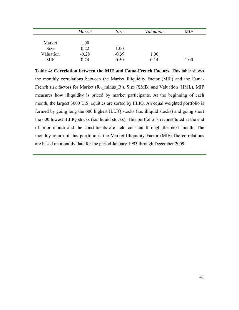
41
Market Size Valuation MIF
Market 1.00 Size 0.22 1.00
Valuation -0.28 -0.39 1.00 MIF 0.24 0.50 0.14 1.00
Table 4: Correlation between the MIF and Fama-French Factors. This table shows
the monthly correlations between the Market Illiquidity Factor (MIF) and the Fama-
French risk factors for Market (Rm_minus_Rf), Size (SMB) and Valuation (HML). MIF
measures how illiquidity is priced by market participants. At the beginning of each
month, the largest 3000 U.S. equities are sorted by IILIQ. An equal weighted portfolio is
formed by going long the 600 highest ILLIQ stocks (i.e. illiquid stocks) and going short
the 600 lowest ILLIQ stocks (i.e. liquid stocks). This portfolio is reconstituted at the end
of prior month and the constituents are held constant through the next month. The
monthly return of this portfolio is the Market Illiquidity Factor (MIF).The correlations
are based on monthly data for the period January 1993 through December 2009.
42
Small ME Big ME Low
BE/ME Medium BE/ME
High BE/ME
Low BE/ME
Medium BE/ME
High BE/ME
Constant 0.00 0.01*** 0.01*** 0.00*** 0.00*** 0.00*
(-0.89) (5.62) (5.24) (2.85) (2.59) (2.25)
Market 1.04*** 0.86*** 0.86*** 1.10*** 1.08*** 1.04*** (21.08) (32.73) (23.46) (39.6) (37.54) (40.56)
Size 0.56*** 0.49*** 0.58*** 0.04 0.02 0.02 (7.33) (12.08) (10.06) (0.87) (0.51) (0.46)
Valuation -0.62*** 0.13*** 0.34*** -0.27*** 0.51*** 0.73*** (-8.35) (3.23) (6.17) (-6.5) (11.83) (18.87)
MIF 0.70*** 0.42*** 0.37*** 0.16*** 0.09* 0.17*** (9.53) (10.95) (6.82) (3.94) (2.02) (4.48)
Adjusted 2
0.88 0.92 0.86 0.92 0.89 0.91
Table 5: Factor Regressions. This table shows the results of contemporaneous
regressions of the returns on the six Fama-French portfolios on various risk factors. The
Fama-French portfolios are the intersections of two portfolios formed on size (market
value of equity or ME) and three portfolios formed on valuation (the ratio of book value
of equity to market value of equity, or BE/ME). The portfolio constituents are equally
weighted. The explanatory variables are the Fama-French risk factors for Market
(Rm_minus_Rf), Size (SMB) and Valuation (HML) and the Market Illiquidity Factor
(MIF). MIF measures the return of illiquid securities relative to liquid securities, and can
be thought of as the market price of illiquidity measured as a return premium. The
regressions are based on monthly data for the period January 1993 through December
2009. t-stats are shown in parenthesis. The asterisk denotes the level of significance.
Single asterisk, double asterisks and triple asterisks denote significance level of 0.05,
0.02 and 0.01, respectively.
43
Figure 3: Liquidity Regimes. This figure describes the four liquidity regimes. Liquidity
regimes are states of market liquidity that are characterized by particular levels of
illiquidity (as measured by MIL) and the pricing of illiquidity by market participants (as
measured by MIF). The Benign Liquidity Regime is defined as an improvement in
liquidity conditions (a negative change in MIL) accompanied by out-performance of
illiquid securities (a positive change in MIF). The Liquidity Crisis Regime is defined as
the deterioration in liquidity conditions (a positive change in MIL) accompanied by
underperformance of illiquid securities (a negative change in MIF). The De-Leveraging
Regime is defined as the deterioration in liquidity conditions (a positive change in MIL)
accompanied by out-performance of illiquid securities (a positive change in MIF). The
Liquidity Correction Regime is defined as an improvement in liquidity conditions
(negative change in MIL) accompanied by underperformance of illiquid securities
(negative change in MIF).
1.0%
1.1%
1.2%
1.3%
1.4%
1.5%
1.6%
90
100
110
120
130
140
150
160
Apr
-200
9
Ma
y-2
009
Jun-
2009
Jul-2
009
Aug
-20
09
Sep
-20
09
MIL
MIF
Benign Liquidity Regime
MIF MIL
1.2%
1.4%
1.6%
1.8%
2.0%
2.2%
2.4%
2.6%
9092949698
100102104106108110
Apr
-199
8
Ma
y-1
998
Jun-
1998
Jul-1
998
Aug
-19
98
Sep
-19
98
MIL
MIF
Liquidity Crisis Regime
MIF MIL
0.9%
1.0%
1.1%
1.2%
1.3%
1.4%
1.5%
1.6%
9092949698
100102104106108110
Jul-2
008
Aug
-20
08
Sep
-20
08
MIL
MIF
De-Leveraging Regime
MIF MIL
1.1%
1.2%1.3%1.4%1.5%1.6%1.7%1.8%1.9%2.0%
85
87
89
91
93
95
97
99
De
c-20
08
Jan-
2009
Feb
-200
9
MIL
MIF
Liquidity Correction Regime
MIF MIL
44
Intercept Illiquidity Level
Change in Illiquidity
Level
Liquidity Risk
Estimate
0.00
0.05***
0.01***
-0.02***
0.02***
-0.05***
-0.10*** (0.00) (8.83) (3.66) (-7.16) (16.02) (-10.56) (-11.84)
Adjusted R2
0.03
Table 6: Fixed Effects Regression of Fama-French Betas and Liquidity Metrics. This
table presents the regression results of the next month’s excess returns against exogenous
variables defined as Fama-French factor loadings for MKT, SMB and HML along with
various liquidity metrics. The liquidity metrics used are the illiquidity level, the change in the
illiquidity level, and liquidity risk. The regressions are performed as fixed effects on 100
portfolios sorted on liquidity level, for the period January 1993 through December 2009. The
portfolio variables are computed as equally-weighted averages. The t-stats are shown in
parenthesis. Single asterisk, double asterisks and triple asterisks denote significance level of
0.05, 0.02 and 0.01, respectively.
45
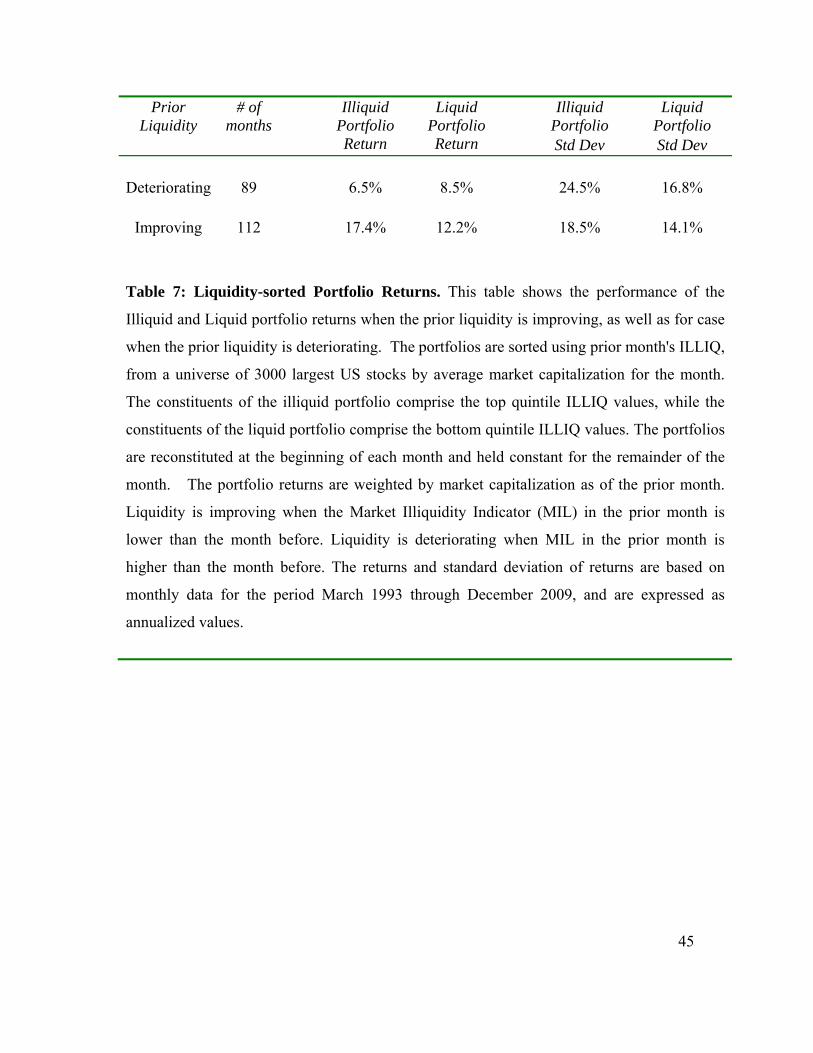
Prior Liquidity
# of months
Illiquid Portfolio
Liquid Portfolio
Illiquid
Portfolio Liquid
Portfolio Return Return Std Dev Std Dev
Deteriorating 89 6.5% 8.5% 24.5% 16.8%
Improving 112 17.4% 12.2% 18.5% 14.1%
Table 7: Liquidity-sorted Portfolio Returns. This table shows the performance of the
Illiquid and Liquid portfolio returns when the prior liquidity is improving, as well as for case
when the prior liquidity is deteriorating. The portfolios are sorted using prior month's ILLIQ,
from a universe of 3000 largest US stocks by average market capitalization for the month.
The constituents of the illiquid portfolio comprise the top quintile ILLIQ values, while the
constituents of the liquid portfolio comprise the bottom quintile ILLIQ values. The portfolios
are reconstituted at the beginning of each month and held constant for the remainder of the
month. The portfolio returns are weighted by market capitalization as of the prior month.
Liquidity is improving when the Market Illiquidity Indicator (MIL) in the prior month is
lower than the month before. Liquidity is deteriorating when MIL in the prior month is
higher than the month before. The returns and standard deviation of returns are based on
monthly data for the period March 1993 through December 2009, and are expressed as
annualized values.
46
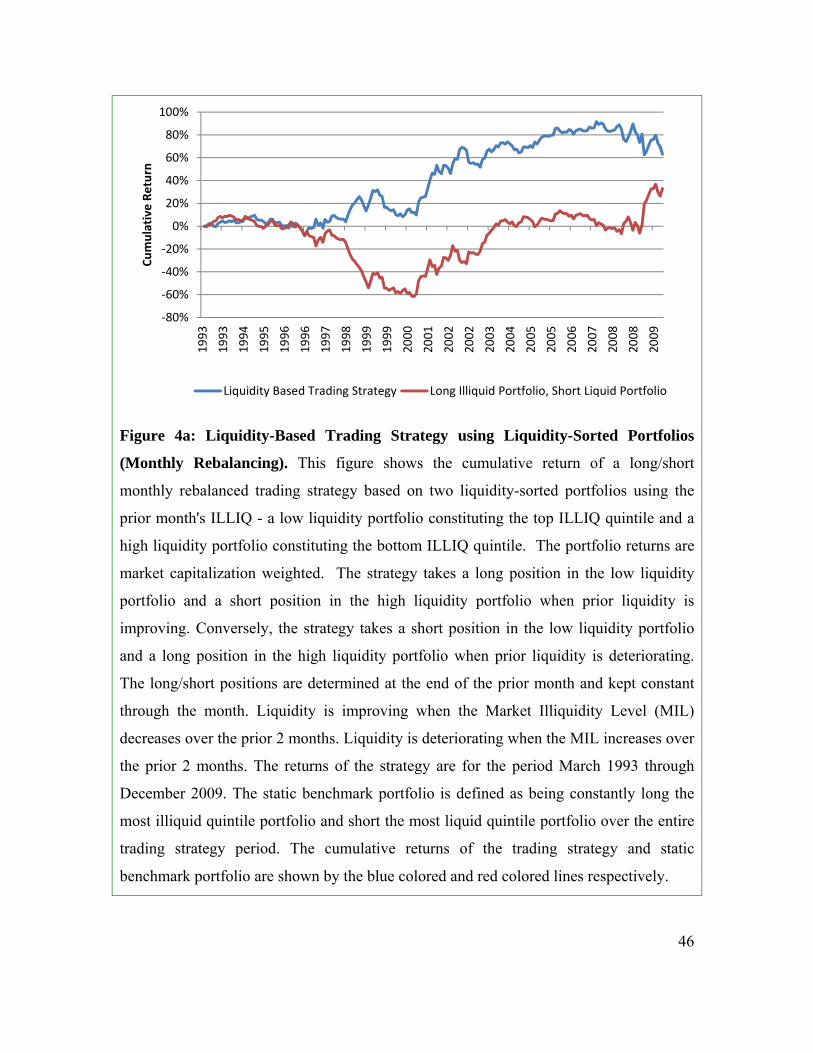
Figure 4a: Liquidity-Based Trading Strategy using Liquidity-Sorted Portfolios
(Monthly Rebalancing). This figure shows the cumulative return of a long/short
monthly rebalanced trading strategy based on two liquidity-sorted portfolios using the
prior month's ILLIQ - a low liquidity portfolio constituting the top ILLIQ quintile and a
high liquidity portfolio constituting the bottom ILLIQ quintile. The portfolio returns are
market capitalization weighted. The strategy takes a long position in the low liquidity
portfolio and a short position in the high liquidity portfolio when prior liquidity is
improving. Conversely, the strategy takes a short position in the low liquidity portfolio
and a long position in the high liquidity portfolio when prior liquidity is deteriorating.
The long/short positions are determined at the end of the prior month and kept constant
through the month. Liquidity is improving when the Market Illiquidity Level (MIL)
decreases over the prior 2 months. Liquidity is deteriorating when the MIL increases over
the prior 2 months. The returns of the strategy are for the period March 1993 through
December 2009. The static benchmark portfolio is defined as being constantly long the
most illiquid quintile portfolio and short the most liquid quintile portfolio over the entire
trading strategy period. The cumulative returns of the trading strategy and static
benchmark portfolio are shown by the blue colored and red colored lines respectively.
‐80%
‐60%
‐40%
‐20%
0%
20%
40%
60%
80%
100%
1993
1993
1994
1995
1996
1996
1997
1998
1999
1999
2000
2001
2002
2002
2003
2004
2005
2005
2006
2007
2008
2008
2009
Cumulative Return
Liquidity Based Trading Strategy Long Illiquid Portfolio, Short Liquid Portfolio
47
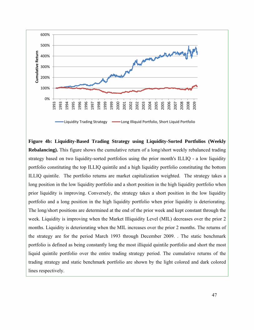
Figure 4b: Liquidity-Based Trading Strategy using Liquidity-Sorted Portfolios (Weekly
Rebalancing). This figure shows the cumulative return of a long/short weekly rebalanced trading
strategy based on two liquidity-sorted portfolios using the prior month's ILLIQ - a low liquidity
portfolio constituting the top ILLIQ quintile and a high liquidity portfolio constituting the bottom
ILLIQ quintile. The portfolio returns are market capitalization weighted. The strategy takes a
long position in the low liquidity portfolio and a short position in the high liquidity portfolio when
prior liquidity is improving. Conversely, the strategy takes a short position in the low liquidity
portfolio and a long position in the high liquidity portfolio when prior liquidity is deteriorating.
The long/short positions are determined at the end of the prior week and kept constant through the
week. Liquidity is improving when the Market Illiquidity Level (MIL) decreases over the prior 2
months. Liquidity is deteriorating when the MIL increases over the prior 2 months. The returns of
the strategy are for the period March 1993 through December 2009. . The static benchmark
portfolio is defined as being constantly long the most illiquid quintile portfolio and short the most
liquid quintile portfolio over the entire trading strategy period. The cumulative returns of the
trading strategy and static benchmark portfolio are shown by the light colored and dark colored
lines respectively.
0%
100%
200%
300%
400%
500%
600%
1993
1993
1994
1995
1996
1996
1997
1998
1999
1999
2000
2001
2002
2002
2003
2004
2005
2005
2006
2007
2008
2008
2009
Cumulative
Return
Liquidity Trading Strategy Long Illiquid Portfolio, Short Liquid Portfolio
48
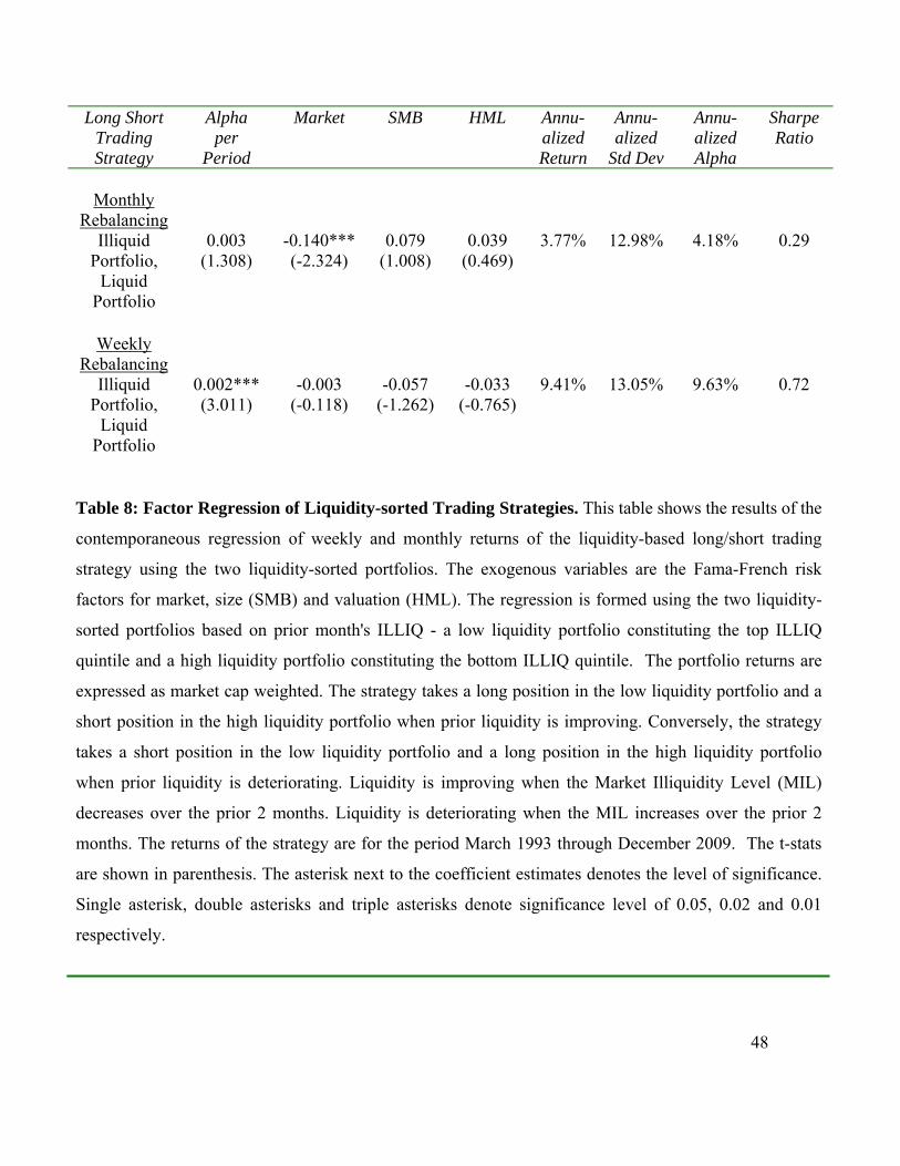
Long Short Trading Strategy
Alpha per
Period
Market SMB HML Annu-alized Return
Annu-alized
Std Dev
Annu-alized Alpha
Sharpe Ratio
Monthly
Rebalancing
Illiquid Portfolio,
Liquid Portfolio
0.003 (1.308)
-0.140*** (-2.324)
0.079 (1.008)
0.039 (0.469)
3.77% 12.98% 4.18% 0.29
Weekly
Rebalancing
Illiquid Portfolio,
Liquid Portfolio
0.002*** (3.011)
-0.003 (-0.118)
-0.057 (-1.262)
-0.033 (-0.765)
9.41% 13.05% 9.63% 0.72
Table 8: Factor Regression of Liquidity-sorted Trading Strategies. This table shows the results of the
contemporaneous regression of weekly and monthly returns of the liquidity-based long/short trading
strategy using the two liquidity-sorted portfolios. The exogenous variables are the Fama-French risk
factors for market, size (SMB) and valuation (HML). The regression is formed using the two liquidity-
sorted portfolios based on prior month's ILLIQ - a low liquidity portfolio constituting the top ILLIQ
quintile and a high liquidity portfolio constituting the bottom ILLIQ quintile. The portfolio returns are
expressed as market cap weighted. The strategy takes a long position in the low liquidity portfolio and a
short position in the high liquidity portfolio when prior liquidity is improving. Conversely, the strategy
takes a short position in the low liquidity portfolio and a long position in the high liquidity portfolio
when prior liquidity is deteriorating. Liquidity is improving when the Market Illiquidity Level (MIL)
decreases over the prior 2 months. Liquidity is deteriorating when the MIL increases over the prior 2
months. The returns of the strategy are for the period March 1993 through December 2009. The t-stats
are shown in parenthesis. The asterisk next to the coefficient estimates denotes the level of significance.
Single asterisk, double asterisks and triple asterisks denote significance level of 0.05, 0.02 and 0.01
respectively.
49
Index Dollar Trading
Volume Market
Cap Bid-Ask
Spread % Illiquidity
Cost
DJIA 846,356,180 95,376,693 0.05% 0.01%
Russell 2000 6,008,233 344,102
0.22%
3.87%
Table 9: Liquidity properties of the Dow Jones Industrial
Average (DJIA) and Russell 2000 Indices. This table reports dollar
trading volume, market capitalization, bid-ask spread% and illiquidity
cost of the Dow Jones Industrial Average (DJIA) and Russell 2000
Indices, for the calendar year 2009, using constituents as of the end of
2008. The median liquidity property estimate is computed each day
for each index. The average value for calendar year 2009 is reported
in the table. Bid-Ask Spread% is calculated as [(ask price - bid
price)/closing price], using daily close values. Illiquidity Cost is the
market impact cost of trading USD 10 million in a trading day and is
estimated using intraday data.
50
Prior Liquidity
# of months
Russell 2000 Return
DJIA Return
Russell 2000
Std Dev DJIA
Std Dev
Deteriorating 89 4.0% 7.1% 22.6% 16.1%
Improving 112 12.3% 9.4% 16.6% 14.2%
Table 10: Prior Liquidity Influences U.S. Equity Index Returns. This table shows the
performance of the Dow Jones Industrial Average (DJIA) and Russell 2000 Index returns
when the prior liquidity is improving as well as for period when the prior liquidity is
deteriorating. Liquidity is improving when the Market Illiquidity Indicator (MIL) in the
prior month is lower than the month before. Liquidity is deteriorating when MIL in the
prior month is higher than the month before. The returns and standard deviation of returns
are based on monthly data for the period January 1993 through December 2009, and are
expressed as annualized values.
51
Figure 5a: Liquidity-Based Index Trading Strategy using Equity Indices (Monthly
Rebalancing). This figure shows the cumulative return of a long/short monthly
rebalanced trading strategy based on the Dow Jones Industrial Average (DJIA) and
Russell 2000 Index. The strategy takes a long position in the Russell 2000 and a short
position in the DJIA when prior liquidity is improving. Conversely, the strategy takes a
short position in the Russell 2000 and a long position in the DJIA when prior liquidity is
deteriorating. The long/short positions are determined at the end of the prior month and
kept constant through the month. Liquidity is improving when the Market Illiquidity
Level (MIL) decreases over the prior 2 months. Liquidity is deteriorating when the MIL
increases over the prior 2 months. The returns of the strategy are for the period March
1993 through December 2009. The static benchmark portfolio is defined as being
constantly long the Russell 2000 Index and being short the DJIA Index over the entire
trading strategy period. The cumulative returns of the trading strategy and static
benchmark portfolio are shown by the blue colored and red colored lines respectively.
‐60%
‐40%
‐20%
0%
20%
40%
60%
80%
100%
1993
1993
1994
1995
1996
1996
1997
1998
1999
1999
2000
2001
2002
2002
2003
2004
2005
2005
2006
2007
2008
2008
2009
Cumulative
Return
Liquidity Based Trading Strategy Long Russell2000, Short DJIA
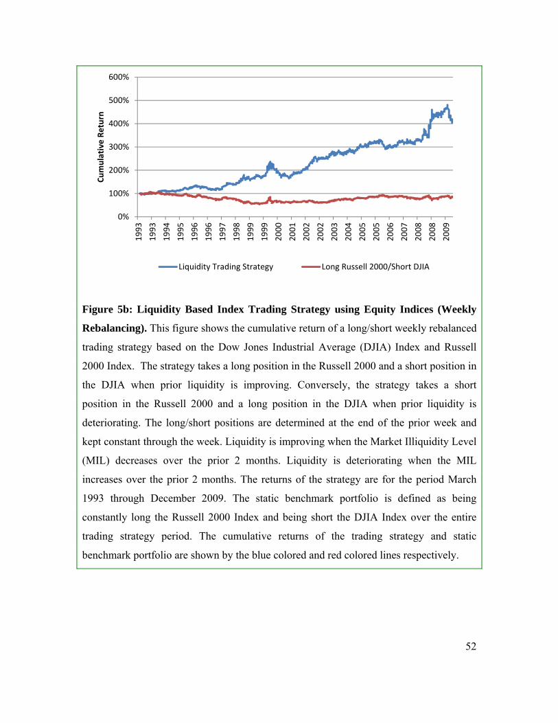
52
Figure 5b: Liquidity Based Index Trading Strategy using Equity Indices (Weekly
Rebalancing). This figure shows the cumulative return of a long/short weekly rebalanced
trading strategy based on the Dow Jones Industrial Average (DJIA) Index and Russell
2000 Index. The strategy takes a long position in the Russell 2000 and a short position in
the DJIA when prior liquidity is improving. Conversely, the strategy takes a short
position in the Russell 2000 and a long position in the DJIA when prior liquidity is
deteriorating. The long/short positions are determined at the end of the prior week and
kept constant through the week. Liquidity is improving when the Market Illiquidity Level
(MIL) decreases over the prior 2 months. Liquidity is deteriorating when the MIL
increases over the prior 2 months. The returns of the strategy are for the period March
1993 through December 2009. The static benchmark portfolio is defined as being
constantly long the Russell 2000 Index and being short the DJIA Index over the entire
trading strategy period. The cumulative returns of the trading strategy and static
benchmark portfolio are shown by the blue colored and red colored lines respectively.
0%
100%
200%
300%
400%
500%
600%
1993
1993
1994
1995
1996
1996
1997
1998
1999
1999
2000
2001
2002
2002
2003
2004
2005
2005
2006
2007
2008
2008
2009
Cumulative Return
Liquidity Trading Strategy Long Russell 2000/Short DJIA
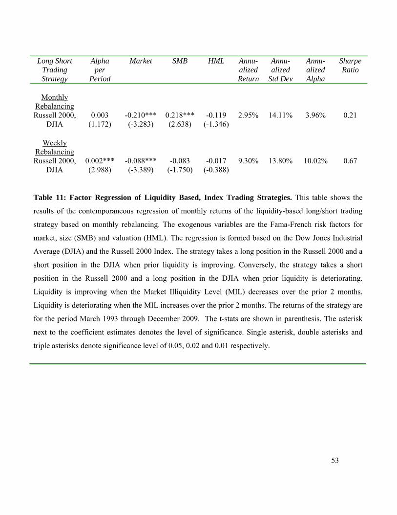
53
Long Short
Trading Strategy
Alpha per
Period
Market SMB HML Annu-alized Return
Annu-alized
Std Dev
Annu-alized Alpha
Sharpe Ratio
Monthly
Rebalancing
Russell 2000, DJIA
0.003 (1.172)
-0.210*** (-3.283)
0.218*** (2.638)
-0.119 (-1.346)
2.95% 14.11% 3.96% 0.21
Weekly
Rebalancing
Russell 2000, DJIA
0.002*** (2.988)
-0.088*** (-3.389)
-0.083 (-1.750)
-0.017 (-0.388)
9.30% 13.80% 10.02% 0.67
Table 11: Factor Regression of Liquidity Based, Index Trading Strategies. This table shows the
results of the contemporaneous regression of monthly returns of the liquidity-based long/short trading
strategy based on monthly rebalancing. The exogenous variables are the Fama-French risk factors for
market, size (SMB) and valuation (HML). The regression is formed based on the Dow Jones Industrial
Average (DJIA) and the Russell 2000 Index. The strategy takes a long position in the Russell 2000 and a
short position in the DJIA when prior liquidity is improving. Conversely, the strategy takes a short
position in the Russell 2000 and a long position in the DJIA when prior liquidity is deteriorating.
Liquidity is improving when the Market Illiquidity Level (MIL) decreases over the prior 2 months.
Liquidity is deteriorating when the MIL increases over the prior 2 months. The returns of the strategy are
for the period March 1993 through December 2009. The t-stats are shown in parenthesis. The asterisk
next to the coefficient estimates denotes the level of significance. Single asterisk, double asterisks and
triple asterisks denote significance level of 0.05, 0.02 and 0.01 respectively.