Embed Size (px)
Citation preview
Portfolio Statistics and OptimizationDistributions and Summary Statistics
chris bemis
January 28, 2021
chris bemis Portfolio Statistics and Optimization
Cumulative Distribution Functions
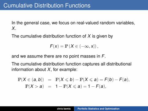
In the general case, we focus on real-valued random variables,X .
The cumulative distribution function of X is given by
F(x) = P (X ∈ (−∞, x]) ,
and we assume there are no point masses in F .
The cumulative distribution function captures all distributionalinformation about X , for example:
P(X ∈ (a,b]) = P(X 6 b) − P(X 6 a) = F(b) − F(a),P(X > a) = 1 − P(X 6 a) = 1 − F(a),
chris bemis Portfolio Statistics and Optimization
Symmetric Distributions and Linear Transformations
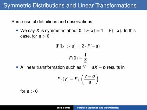
Some useful definitions and observations
• We say X is symmetric about 0 if F(x) = 1 − F(−x). In thiscase, for a > 0,
P(|x | > a) = 2 · F(−a)
F(0) =12
• A linear transformation such as Y = aX + b results in
FY (y) = FX
(y − b
a
)for a > 0
chris bemis Portfolio Statistics and Optimization
Probability Density Functions
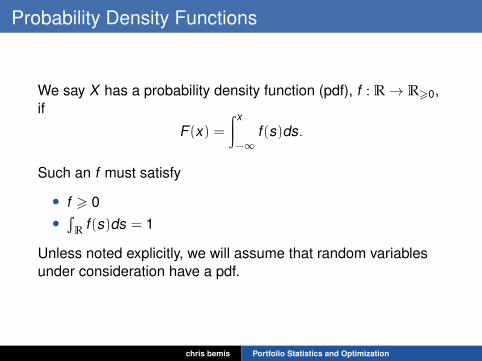
We say X has a probability density function (pdf), f : R→ R>0,if
F(x) =∫ x
−∞ f(s)ds.
Such an f must satisfy
• f > 0•∫R f(s)ds = 1
Unless noted explicitly, we will assume that random variablesunder consideration have a pdf.
chris bemis Portfolio Statistics and Optimization
Expectation and Variance
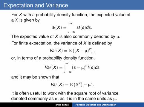
For X with a probability density function, the expected value ofa X is given by
E(X) =
∫∞−∞ sf(s)ds.
The expected value of X is also commonly denoted by µ.
For finite expectation, the variance of X is defined by
Var(X) = E((X − µ)2) ,
or, in terms of a probability density function,
Var(X) =
∫∞−∞(s − µ)2f(s)ds
and it may be shown that
Var(X) = E(X2)− µ2.
It is often useful to work with the square root of variance,denoted commonly as σ, as it is in the same units as µ.
chris bemis Portfolio Statistics and Optimization
Linear Transformations and Expectation and Variance
Shifting and dilating X results in changes to the expectationand variance as
E(aX + b) = aE(X) + b
Var(aX + b) = a2Var(X).
The expectation operator is therefore linear. And variance,sometimes called the dispersion parameter of X , isindependent of the location of the origin.
chris bemis Portfolio Statistics and Optimization
Skew and Kurtosis
In addition to the location and dispersion measures ofexpectation and variance, higher moments are sometimesconsidered.
The skew of X is defined as
γ = E
((X − µ)3
σ3
)and the kurtosis of X is given by
κ = E
((X − µ)4
σ4
).
More negative (positive) skew indicates more mass to the left(right) of the mean.
Kurtosis is a very rough indication of how much mass is in thetails of the distribution of X , with a higher value indicating fattertails.
chris bemis Portfolio Statistics and Optimization

Percentiles
The (100 · p)th percentile of X is given by
πp = min{π |F(π) = p}.
and if F is locally invertible near πp, then πp = F−1(p).
In contrast to the mean, variance, skew, or kurtosis of X ,percentiles are never infinite.
Several percentile-based risk metrics are used in portfolioconstruction, like Value-at-Risk, and Conditional Value-at-Risk.
chris bemis Portfolio Statistics and Optimization
Multivariate Distributions
We also consider random variables in RN as
X =
X1X2...
XN
.
And, as before, define now a joint cumulative distributionfunction of X , F : RN → [0,1] as
F(x1, x2, . . . , xN) = P (X1 6 x1,X2 6 x2, . . . ,XN 6 xN) .
chris bemis Portfolio Statistics and Optimization
Multivariate Density
Again, we focus primarily on random variables which admit aprobability density function, now,
f : RN → R+,
with
F(x1, x2, . . . , xN) =
∫ x1
−∞ · · ·∫ xN
−∞ f(s1, . . . , sN)dsN · · ·ds1
as expected.
The same requirements for this f as before apply.
chris bemis Portfolio Statistics and Optimization
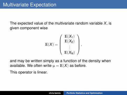
Multivariate Expectation
The expected value of the multivariate random variable X , isgiven component wise
E(X) =
E(X1)E(X2)
...E(XN)
,
and may be written simply as a function of the density whenavailable. We often write µ = E(X) as before.
This operator is linear.
chris bemis Portfolio Statistics and Optimization
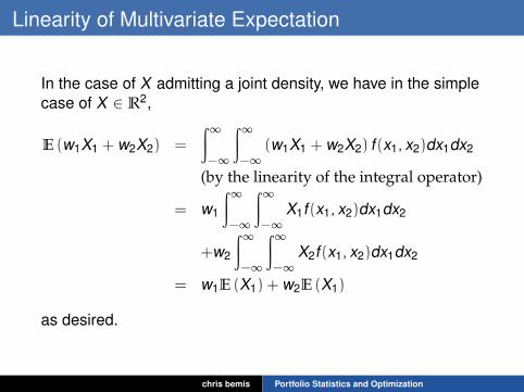
Linearity of Multivariate Expectation
In the case of X admitting a joint density, we have in the simplecase of X ∈ R2,
E (w1X1 + w2X2) =
∫∞−∞∫∞−∞ (w1X1 + w2X2) f(x1, x2)dx1dx2
(by the linearity of the integral operator)
= w1
∫∞−∞∫∞−∞ X1f(x1, x2)dx1dx2
+w2
∫∞−∞∫∞−∞ X2f(x1, x2)dx1dx2
= w1E (X1) + w2E (X1)
as desired.
chris bemis Portfolio Statistics and Optimization
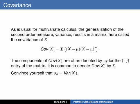
Covariance
As is usual for multivariate calculus, the generalization of thesecond order measure, variance, results in a matrix, here calledthe covariance of X ,
Cov(X) = E((X − µ)(X − µ) ′
).
The components of Cov(X) are often denoted by σij for the (i, j)entry of the matrix. It is common to denote Cov(X) by Σ.
Convince yourself that σii = Var(Xi).
chris bemis Portfolio Statistics and Optimization
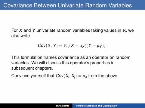
Covariance Between Univariate Random Variables
For X and Y univariate random variables taking values in R, wealso write
Cov(X ,Y) = E ((X − µX )(Y − µY )) .
This formulation frames covariance as an operator on randomvariables. We will discuss this operator’s properties insubsequent chapters.
Convince yourself that Cov(Xi ,Xj) = σij from the above.
chris bemis Portfolio Statistics and Optimization
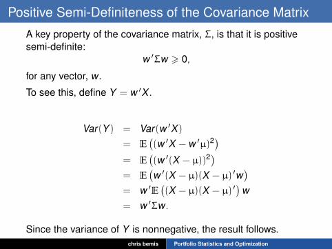
Positive Semi-Definiteness of the Covariance Matrix
A key property of the covariance matrix, Σ, is that it is positivesemi-definite:
w ′Σw > 0,
for any vector, w.
To see this, define Y = w ′X .
Var(Y) = Var(w ′X)
= E((w ′X − w ′µ)2)
= E((w ′(X − µ))2)
= E(w ′(X − µ)(X − µ) ′w
)= w ′E
((X − µ)(X − µ) ′
)w
= w ′Σw.
Since the variance of Y is nonnegative, the result follows.chris bemis Portfolio Statistics and Optimization
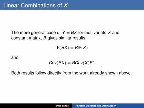
Linear Combinations of X
The more general case of Y = BX for multivariate X andconstant matrix, B gives similar results:
E(BX) = BE(X)
andCov(BX) = BCov(X)B ′.
Both results follow directly from the work already shown above.
chris bemis Portfolio Statistics and Optimization
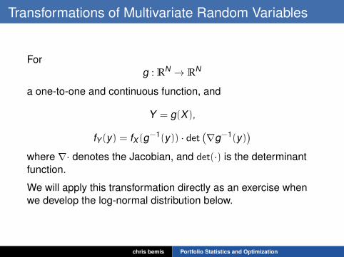
Transformations of Multivariate Random Variables
Forg : RN → RN
a one-to-one and continuous function, and
Y = g(X),
fY (y) = fX (g−1(y)) · det(∇g−1(y)
)where ∇· denotes the Jacobian, and det(·) is the determinantfunction.
We will apply this transformation directly as an exercise whenwe develop the log-normal distribution below.
chris bemis Portfolio Statistics and Optimization

Marginals
The marginal distribution of Xj is denoted
Fj(xj) = P(Xj 6 xj)
and is given byF(∞, . . . , xj , . . . ,∞) .
When a density exists for X , the marginal density for Xj is givenby
fj(x) =∫∞−∞ · · ·
∫∞−∞ f(s1, . . . , x, . . . , sN)dsN · · ·dsj+1dsj−1 · · ·ds1
chris bemis Portfolio Statistics and Optimization
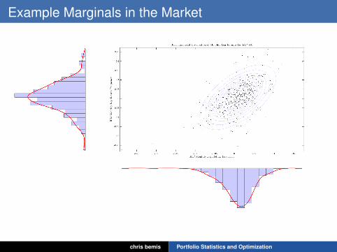
Example Marginals in the Market
chris bemis Portfolio Statistics and Optimization
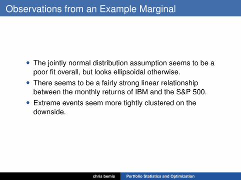
Observations from an Example Marginal
• The jointly normal distribution assumption seems to be apoor fit overall, but looks ellipsoidal otherwise.• There seems to be a fairly strong linear relationship
between the monthly returns of IBM and the S&P 500.• Extreme events seem more tightly clustered on the
downside.
chris bemis Portfolio Statistics and Optimization
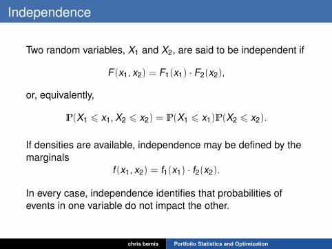
Independence
Two random variables, X1 and X2, are said to be independent if
F(x1, x2) = F1(x1) · F2(x2),
or, equivalently,
P(X1 6 x1,X2 6 x2) = P(X1 6 x1)P(X2 6 x2).
If densities are available, independence may be defined by themarginals
f(x1, x2) = f1(x1) · f2(x2).
In every case, independence identifies that probabilities ofevents in one variable do not impact the other.
chris bemis Portfolio Statistics and Optimization
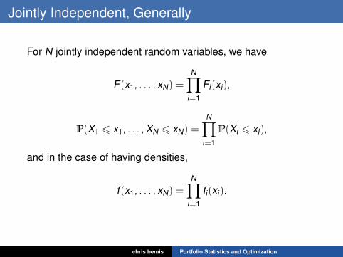
Jointly Independent, Generally
For N jointly independent random variables, we have
F(x1, . . . , xN) =
N∏i=1
Fi(xi),
P(X1 6 x1, . . . ,XN 6 xN) =
N∏i=1
P(Xi 6 xi),
and in the case of having densities,
f(x1, . . . , xN) =
N∏i=1
fi(xi).
chris bemis Portfolio Statistics and Optimization
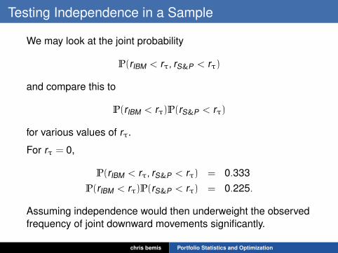
Testing Independence in a Sample
We may look at the joint probability
P(rIBM < rτ, rS&P < rτ)
and compare this to
P(rIBM < rτ)P(rS&P < rτ)
for various values of rτ.
For rτ = 0,
P(rIBM < rτ, rS&P < rτ) = 0.333P(rIBM < rτ)P(rS&P < rτ) = 0.225.
Assuming independence would then underweight the observedfrequency of joint downward movements significantly.
chris bemis Portfolio Statistics and Optimization
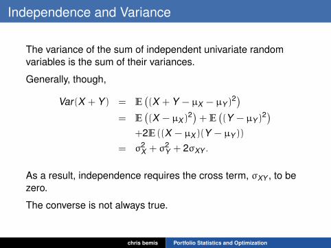
Independence and Variance
The variance of the sum of independent univariate randomvariables is the sum of their variances.
Generally, though,
Var(X + Y) = E((X + Y − µX − µY )
2)= E
((X − µX )
2)+ E ((Y − µY )2)
+2E ((X − µX )(Y − µY ))
= σ2X + σ2
Y + 2σXY .
As a result, independence requires the cross term, σXY , to bezero.
The converse is not always true.
chris bemis Portfolio Statistics and Optimization
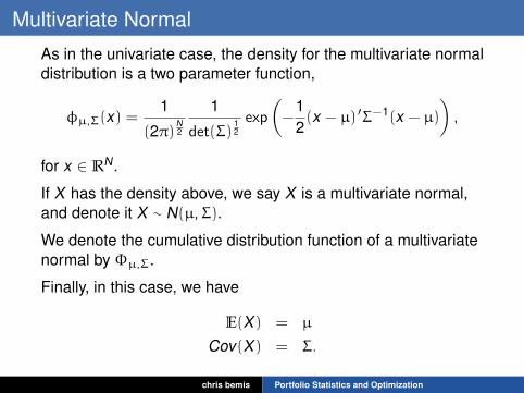
Multivariate Normal
As in the univariate case, the density for the multivariate normaldistribution is a two parameter function,
φµ,Σ(x) =1
(2π)N2
1
det(Σ)12exp
(−
12(x − µ) ′Σ−1(x − µ)
),
for x ∈ RN.
If X has the density above, we say X is a multivariate normal,and denote it X ∼ N(µ,Σ).
We denote the cumulative distribution function of a multivariatenormal by Φµ,Σ.
Finally, in this case, we have
E(X) = µ
Cov(X) = Σ.
chris bemis Portfolio Statistics and Optimization
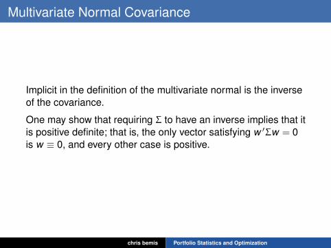
Multivariate Normal Covariance
Implicit in the definition of the multivariate normal is the inverseof the covariance.
One may show that requiring Σ to have an inverse implies that itis positive definite; that is, the only vector satisfying w ′Σw = 0is w ≡ 0, and every other case is positive.
chris bemis Portfolio Statistics and Optimization
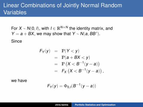
Linear Combinations of Jointly Normal RandomVariables
For X ∼ N(0, I), with I ∈ RN×N the identity matrix, andY = a + BX , we may show that Y ∼ N(a,BB ′).
Since
FY (y) = P(Y < y)= P(a + BX < y)= P
(X < B−1(y − a)
)= FX
(X < B−1(y − a)
),
we haveFY (y) = Φ0,I(B−1(y − a))
chris bemis Portfolio Statistics and Optimization

Linear Combinations of Jointly Normal RandomVariables
Resorting to the density, and using the ‘proportional to’notation, ∝ to avoid the normalizing scalar, we have
FY (y) ∝∫
s6B−1(y−a)exp
(−
12
s ′s)
ds
(changing variables x = Bs + a,1
det (B)dx = ds)
=1
det (B)
∫x6y
exp
(−
12(B−1(x − a)) ′(B−1(x − a))
)dx
=1
det (B)
∫x6y
exp
(−
12(x − a) ′(B−1) ′B−1(x − a)
)dx
=1
det (B)
∫x6y
exp
(−
12(x − a) ′(BB ′)−1(x − a)
)dx
chris bemis Portfolio Statistics and Optimization
Linear Combinations of Jointly Normal RandomVariables
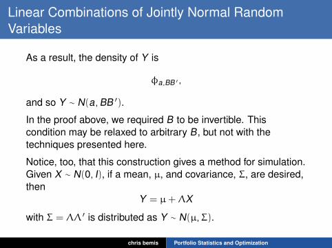
As a result, the density of Y is
φa,BB ′ ,
and so Y ∼ N(a,BB ′).
In the proof above, we required B to be invertible. Thiscondition may be relaxed to arbitrary B, but not with thetechniques presented here.
Notice, too, that this construction gives a method for simulation.Given X ∼ N(0, I), if a mean, µ, and covariance, Σ, are desired,then
Y = µ+ΛX
with Σ = ΛΛ ′ is distributed as Y ∼ N(µ,Σ).
chris bemis Portfolio Statistics and Optimization
Multivariate Log-Normal
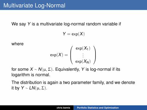
We say Y is a multivariate log-normal random variable if
Y = exp(X)
where
exp(X) =
exp(X1)...
exp(XN)
for some X ∼ N(µ,Σ). Equivalently, Y is log-normal if itslogarithm is normal.
The distribution is again a two parameter family, and we denoteit by Y ∼ LN(µ,Σ).
chris bemis Portfolio Statistics and Optimization
Multivariate Log-Normal Density
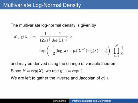
The multivariate log-normal density is given by
lnµ,Σ(x) =1
(2π)N2
1
det(Σ)−12×
exp
(−
12(log(x) − µ) ′Σ−1(log(x) − µ)
)·
N∏i=1
1xi
and may be derived using the change of variable theorem.
Since Y = exp(X), we use g(·) = exp(·).
We are left to gather the inverse and Jacobian of g(·).
chris bemis Portfolio Statistics and Optimization
Multivariate Log-Normal Density
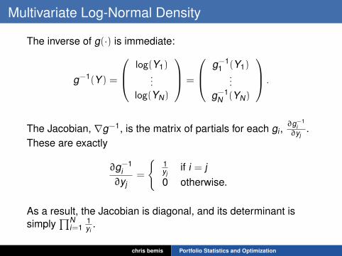
The inverse of g(·) is immediate:
g−1(Y) =
log(Y1)...
log(YN)
=
g−11 (Y1)
...
g−1N (YN)
.
The Jacobian, ∇g−1, is the matrix of partials for each gi ,∂g−1
i∂yj
.These are exactly
∂g−1i∂yj
=
{1yj
if i = j0 otherwise.
As a result, the Jacobian is diagonal, and its determinant issimply
∏Ni=1
1yi
.
chris bemis Portfolio Statistics and Optimization
Multivariate Log-Normal Density
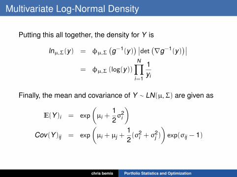
Putting this all together, the density for Y is
lnµ,Σ(y) = φµ,Σ(g−1(y)
) ∣∣det (∇g−1(y))∣∣
= φµ,Σ (log(y))N∏
i=1
1yi
Finally, the mean and covariance of Y ∼ LN(µ,Σ) are given as
E(Y)i = exp
(µi +
12σ2
i
)Cov(Y)ij = exp
(µi + µj +
12(σ2
i + σ2j )
)exp(σij − 1)
chris bemis Portfolio Statistics and Optimization
Multivariate Student t
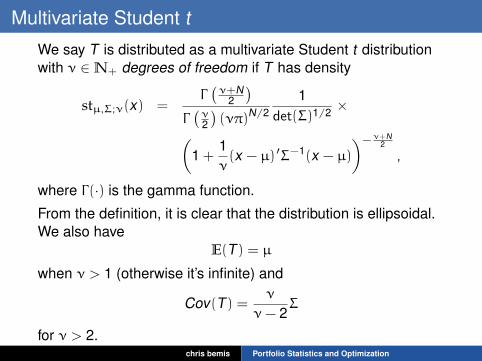
We say T is distributed as a multivariate Student t distributionwith ν ∈N+ degrees of freedom if T has density
stµ,Σ;ν(x) =Γ(ν+N
2
)Γ(ν2
)(νπ)N/2
1det(Σ)1/2 ×(
1 +1ν(x − µ) ′Σ−1(x − µ)
)−ν+N2
,
where Γ(·) is the gamma function.
From the definition, it is clear that the distribution is ellipsoidal.We also have
E(T) = µ
when ν > 1 (otherwise it’s infinite) and
Cov(T) =ν
ν− 2Σ
for ν > 2.chris bemis Portfolio Statistics and Optimization
Linear Transformations of Multivariate Student t
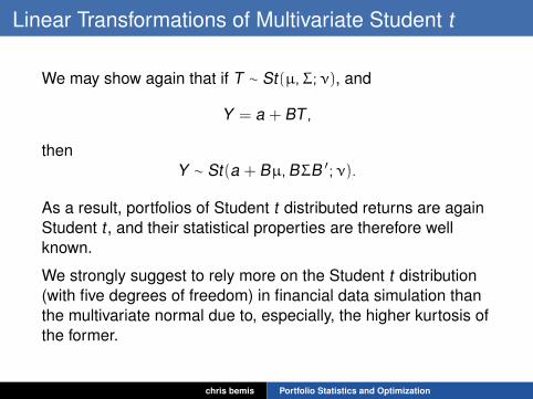
We may show again that if T ∼ St(µ,Σ;ν), and
Y = a + BT ,
thenY ∼ St(a + Bµ,BΣB ′;ν).
As a result, portfolios of Student t distributed returns are againStudent t , and their statistical properties are therefore wellknown.
We strongly suggest to rely more on the Student t distribution(with five degrees of freedom) in financial data simulation thanthe multivariate normal due to, especially, the higher kurtosis ofthe former.
chris bemis Portfolio Statistics and Optimization
Estimators and Convergence
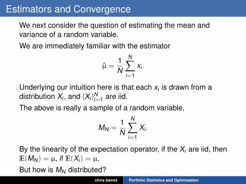
We next consider the question of estimating the mean andvariance of a random variable.We are immediately familiar with the estimator
µ̂ =1N
N∑i=1
xi .
Underlying our intuition here is that each xi is drawn from adistribution Xi , and {Xi}
Ni=1 are iid.
The above is really a sample of a random variable,
MN =1N
N∑i=1
Xi .
By the linearity of the expectation operator, if the Xi are iid, thenE(MN) = µ, if E(Xi) = µ.But how is MN distributed?
chris bemis Portfolio Statistics and Optimization
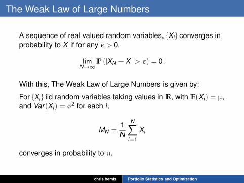
The Weak Law of Large Numbers
A sequence of real valued random variables, {Xi} converges inprobability to X if for any ε > 0,
limN→∞P (|XN − X | > ε) = 0.
With this, The Weak Law of Large Numbers is given by:
For {Xi} iid random variables taking values in R, with E(Xi) = µ,and Var(Xi) = σ
2 for each i,
MN =1N
N∑i=1
Xi
converges in probability to µ.
chris bemis Portfolio Statistics and Optimization
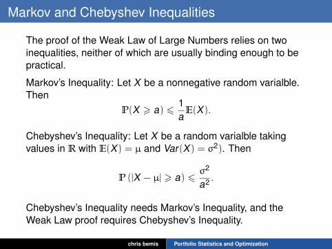
Markov and Chebyshev Inequalities
The proof of the Weak Law of Large Numbers relies on twoinequalities, neither of which are usually binding enough to bepractical.
Markov’s Inequality: Let X be a nonnegative random varialble.Then
P(X > a) 61aE(X).
Chebyshev’s Inequality: Let X be a random varialble takingvalues in R with E(X) = µ and Var(X) = σ2). Then
P (|X − µ| > a) 6σ2
a2 .
Chebyshev’s Inequality needs Markov’s Inequality, and theWeak Law proof requires Chebyshev’s Inequality.
chris bemis Portfolio Statistics and Optimization
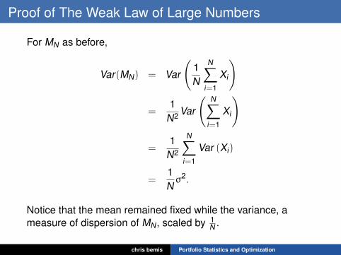
Proof of The Weak Law of Large Numbers
For MN as before,
Var(MN) = Var
(1N
N∑i=1
Xi
)
=1
N2 Var
(N∑
i=1
Xi
)
=1
N2
N∑i=1
Var (Xi)
=1Nσ2.
Notice that the mean remained fixed while the variance, ameasure of dispersion of MN, scaled by 1
N .
chris bemis Portfolio Statistics and Optimization
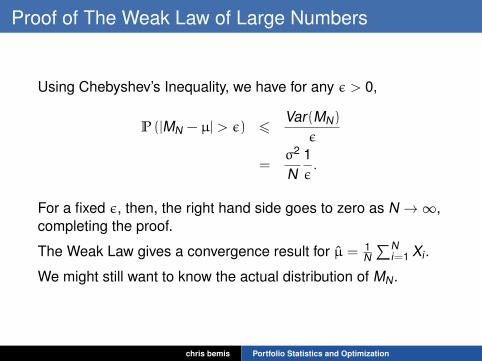
Proof of The Weak Law of Large Numbers
Using Chebyshev’s Inequality, we have for any ε > 0,
P (|MN − µ| > ε) 6Var(MN)
ε
=σ2
N1ε.
For a fixed ε, then, the right hand side goes to zero as N →∞,completing the proof.
The Weak Law gives a convergence result for µ̂ = 1N∑N
i=1 Xi .
We might still want to know the actual distribution of MN.
chris bemis Portfolio Statistics and Optimization
Convergence in Distribution
A sequence of real valued random variables {Xi} withdistribution functions {Fi(·)}, respectively, converges indistribution to X if
limN→∞FN(X) = F(X),
where F(·) is the distribution function of X .
Convergence in probability implies convergence in distributionin the sense that if real valued random variables {Xi} withdistribution functions {Fi(·)} converge in probability to X ,
XN → X
thenFN → F .
chris bemis Portfolio Statistics and Optimization
Central Limit Theorem
For {Xi} iid real random variables with finite mean and variance,µ and σ2, respectively, the cumulative distribution function, FN,of the random variable
ZN =
√N(MN − µ)
σ
satisfieslim
N→∞FN(x) = Φ(x).
That is, the cumulative distribution function of ZN converges indistribution to the standard normal.
While the proof is outside the scope of our work, its usefulnessand ubiquity make it unavoidable.
chris bemis Portfolio Statistics and Optimization
Bias
For a quantity to be estimated, θ, and estimator, θ̂, the bias of θ̂is
Bias(θ̂) = E(θ̂) − θ.
An unbiased estimator has zero bias and satisfies
E(θ̂) = θ.
We have already seen that
MN =1N
N∑i=1
Xi
is an unbiased estimator of the mean.
chris bemis Portfolio Statistics and Optimization
Unbiased Estimator of Variance
With the same assumptions as above,
sN =1
N − 1
N∑i=1
(Xi − µ̂)2,
with µ̂ = 1N∑N
i=1 Xi is an unbiased estimator of the variance ofX . That is,
E(sN) = σ2.
The term 1/(N − 1) is somewhat surprising on first pass. It willbe slightly more intuitive when we encounter the estimate ofvariance again in ordinary least squares where degrees offreedom will be given more color.
chris bemis Portfolio Statistics and Optimization
Proof of Unbiased Estimator of Variance
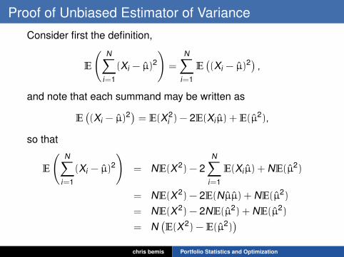
Consider first the definition,
E
(N∑
i=1
(Xi − µ̂)2
)=
N∑i=1
E((Xi − µ̂)
2) ,and note that each summand may be written as
E((Xi − µ̂)
2) = E(X2i ) − 2E(Xiµ̂) + E(µ̂
2),
so that
E
(N∑
i=1
(Xi − µ̂)2
)= NE(X2) − 2
N∑i=1
E(Xiµ̂) + NE(µ̂2)
= NE(X2) − 2E(Nµ̂µ̂) + NE(µ̂2)
= NE(X2) − 2NE(µ̂2) + NE(µ̂2)
= N(E(X2) − E(µ̂2)
)chris bemis Portfolio Statistics and Optimization
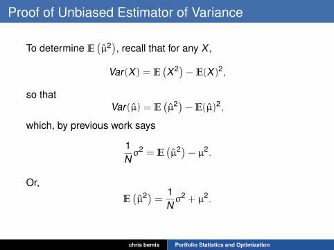
Proof of Unbiased Estimator of Variance
To determine E(µ̂2), recall that for any X ,
Var(X) = E(X2)− E(X)2,
so thatVar(µ̂) = E
(µ̂2)− E(µ̂)2,
which, by previous work says
1Nσ2 = E
(µ̂2)− µ2.
Or,
E(µ̂2) = 1
Nσ2 + µ2.
chris bemis Portfolio Statistics and Optimization
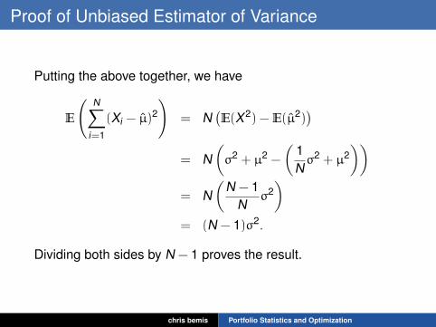
Proof of Unbiased Estimator of Variance
Putting the above together, we have
E
(N∑
i=1
(Xi − µ̂)2
)= N
(E(X2) − E(µ̂2)
)= N
(σ2 + µ2 −
(1Nσ2 + µ2
))= N
(N − 1
Nσ2)
= (N − 1)σ2.
Dividing both sides by N − 1 proves the result.
chris bemis Portfolio Statistics and Optimization
Some Notes on Estimators
Whenever a fit of a distribution has been shown, we haveestimated the mean and variance (and covariance in one case)of the underlying distributions using the above estimators.
Implicit in this estimation is that the random variables underconsideration are iid.
Specifically, we repeatedly assumed, then, that daily log returnsof the S&P are independent. But this may not obtain; see, forexample Amir Khandani and Andrew Lo.
We don’t present a solution to the apparent lack ofindependence of daily returns here, but find it important to notethe tension between estimation in practice, theory, andempirical findings.
chris bemis Portfolio Statistics and Optimization
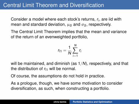
Central Limit Theorem and Diversification
Consider a model where each stock’s returns, ri , are iid withmean and standard deviation, µS and σS , respectively.
The Central Limit Theorem implies that the mean and varianceof the return of an evenweighted portfolio,
rΠ =1N
N∑i=1
ri
will be maintained, and diminish (as 1/N), respectively, and thatthe distribution of rΠ will be normal.
Of course, the assumptions do not hold in practice.
As a prologue, though, we have some motivation to considerdiversification, as such, when constructing a portfolio.
chris bemis Portfolio Statistics and Optimization
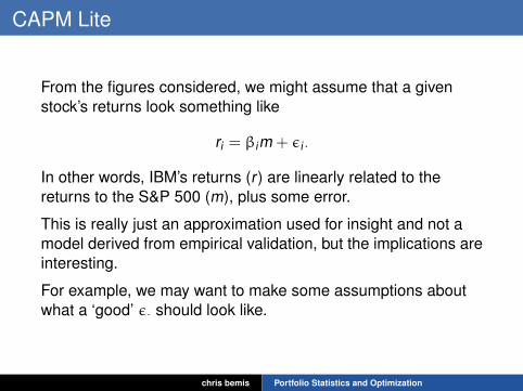
CAPM Lite
From the figures considered, we might assume that a givenstock’s returns look something like
ri = βim + εi .
In other words, IBM’s returns (r) are linearly related to thereturns to the S&P 500 (m), plus some error.
This is really just an approximation used for insight and not amodel derived from empirical validation, but the implications areinteresting.
For example, we may want to make some assumptions aboutwhat a ‘good’ ε· should look like.
chris bemis Portfolio Statistics and Optimization
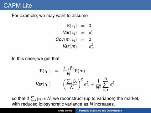
CAPM Lite
For example, we may want to assume
E(εi) = 0Var(εi) = σ2
i
Cov(m, εi) = 0Var(m) = σ2
m.
In this case, we get that
E(rΠ) =
∑i βi
NE(m)
Var(rΠ) =
(∑i βi
N
)2
σ2m +
1N2
N∑i=1
σ2i ,
so that if∑
i βi ≈ N, we reconstruct (up to variance) the market,with reduced idiosyncratic variance as N increases.
chris bemis Portfolio Statistics and Optimization
CAPM Lite
Of course, the attractiveness of reducing idiosyncratic noiseraises the question: Why not just own the market, then?
We will encounter this question again when we have more toolsunder our belt.
chris bemis Portfolio Statistics and Optimization

fin.
chris bemis Portfolio Statistics and Optimization