Power Quality Data Compression - InTech - Opencdn.intechopen.com/pdfs/44193/InTech-Power_quality... · Power Quality Data Compression ... A D D A D D D = + = + + = + + + (8) The decomposition

Chapter 1

Power Quality Data Compression

Gabriel Găşpăresc

Additional information is available at the end of the chapter

http://dx.doi.org/10.5772/53059

1. Introduction

Nowadays we assist to the increasing of devices and equipments connected to power sys‐tems (non-linear loads, industrial rectifiers and inverters, solid-state switching devices, com‐puters, peripheral devices etc). Hence, the parameters of the power supply should beaccurately estimated and monitorized. For this purpose have been proposed power qualitymonitoring systems that are abble to automatically detect and classify disturbances. Theyare using the most recent signal processing techniques for power quality analysis (Bollen etal., 2006), (Dungan et al., 2004), (Lin et al., 2009).

A power quality monitoring system provides huge volume of raw data from different loca‐tions, acquired during long periods of time and the amount of data is increasing daily. Thehardware of a power quality monitoring systems should have a high sampling rate becausethe power quality events cover a broad frequency range, starting from a few Hz (flicker) to afew MHz (transient phenomenon). A high sampling rate leads to large volume of aquireddata (for example, one recorded event could requires megabytes of storage space) whichshould be transferred and stored. Therefore, it is necessary data compression to save storingspace and to reduce the communication time. Any compression methode is a compromisebetween the resulted volume of data and the remained information. The aim is to obtain thesmalest size with the highest information level (Barrera Nunez et al., 2008), (Lorio et al.,2004), (Wang et al., 2005).

In order to compress data there are many approaches used in digital communicationsand image compression. These may be divided in two broad categories: lossless andlossy techniques. The first category keep the signal information intact. The second cate‐gory remove redundant information from signals to achieve a higher compression ratio(Ribeiro et al., 2004).

© 2013 Găşpăresc; licensee InTech. This is an open access article distributed under the terms of the CreativeCommons Attribution License (http://creativecommons.org/licenses/by/3.0), which permits unrestricted use,distribution, and reproduction in any medium, provided the original work is properly cited.

In recent years, the results presented in scientific literature show that the most usedcompression methods in power quality are based on wavelet transform and Slantlettransform. This chapter will provide an overview of their applications for power qualitysignals.

2. Data compression using wavelet transform

2.1. Wavelet transform

The wavelet transform ensures a progressive resolution in time-frequency domain, suitableto track the nonstationary signals dynamics properly. It use a variable window size, widefor low frequencies and narrow for high frequencies, to achieve a good localization in timeand frequency domains (Ribeiro et al., 2007), (Zhang et al., 2011).

The Continuous Wavelet Transform (CWT) of a signal f (t)∈ L 2 R is defined as

,( , ) ( ) ( )tCWT f t dtt gtt g

g

¥

-¥

-= Yò (1)

where τ is the scale factor, γ is the translation factor and Ψτ,γ is the mother wavelet.

The Fourier analysis decomposes a signal into a sum of harmonics and wavelet analysis intoset of functions called wavelets. A wavelet is a waveform of limited duration, usually irreg‐ular and asymmetric. These functions are obtained by dilations and translations of a uniquefunction called mother wavelet Ψτ,γ and the function set (Ψτ,γ) is called the wavelet family

,1( ) ( ), 0,tt Rt g

t g tgg-

Y = Y > Î (2)

The Inverse Continuous Wavelet Transform (ICWT) is given as

, 21( ) ( , ) ( ) d df t CWT t

C t gt gt gt

¥ ¥

Y -¥ -¥

= Yò ò (3)

where CΨ is the normalized constant.

In power quality analysis we work with acquired signals. These are discrete-time signals.Moreover, the CWT provides a redundant signal reprezentation in continuous-time, becausethe initial signal is possible to be reconstructed by a discrete version of CWT. The CWT isevaluated at dyadic intervals: the factor τ and γ are discretezed as τ=2k, γ=2kn where n,kєZ.The relation (2) becomes (Dash et al., 2007), (Qian, 2002)

Power Quality Issues2

/2, ( ) 2 (2 )k k

k n t t nY = Y - (4)

The wavelet transform is the most used multiresolution analysis (MRA) technique of sig‐nals. Multiresolutions signal decompositon is based on subbads decomposition using low-pass filtering and high-pass filtering.

In muliresolution analysis a continuous function x(t) is decomposed as follows

0

00

( ) ( ) ( )j

j jj

x t A t D t=

= +å (5)

where

,( ) ( ) ( )j j j kk

A t c k tj=å (6)

,( ) ( ) ( )j j j kk

D t d k ty=å (7)

cj(k) are the scaling function coefficients, dj(k) are the wavelet function coefficients, j0 is thescale, φ(t) is the scaling function, Aj(t) is called approximation at level j and Dj(t) is called thedetail at level j (Azam et al., 2004), (Zhang et al., 2011).

For a given signal x(t) and a three levels wavelet decomposition the relation (5) become

1 1

2 2 1

3 3 2 1

( ) .

x t A DA D DA D D D

= += + += + + +

(8)

The decomposition of signal x(t) in A1 and D1 is the first decomposition level. At each de‐composition level the signal is decomposed into an approximation and a detail.

Each detail Dj reveals details of the signal and each approximation Aj shows corse information.If the analysed signal contains a high frequency event (for instance, a transient phenomenon),the magnitude of details Dj associated with the event are significant larger than the rest of thecoefficients. This observation is useful for compressing power quality signals: only the detailsDj associated with the events are retained and all other coefficients are discarded. Moreover,the approximation coefficient is also kept for signal reconstruction (Santoso et al., 1997).

2.2. Data compression with wavelet transform

A general data compression method based on wavelet decomposition and reconstruction isshown in Fig. 1. That is a lossy compression method which includes certain steps (Wu et al.,

Power Quality Data Compressionhttp://dx.doi.org/10.5772/53059

3

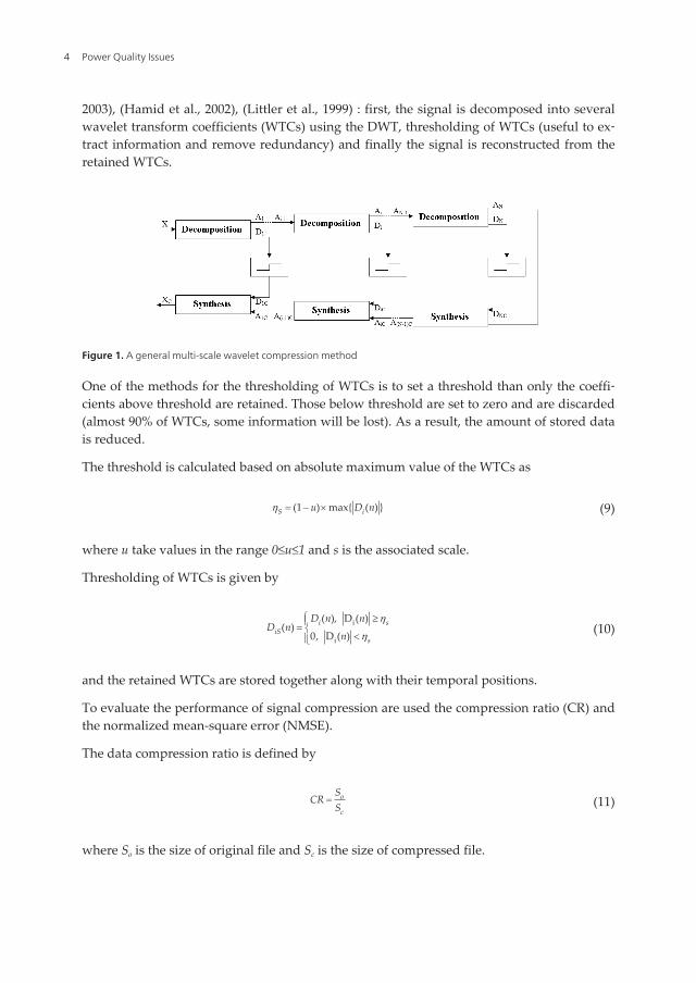
2003), (Hamid et al., 2002), (Littler et al., 1999) : first, the signal is decomposed into severalwavelet transform coefficients (WTCs) using the DWT, thresholding of WTCs (useful to ex‐tract information and remove redundancy) and finally the signal is reconstructed from theretained WTCs.

Figure 1. A general multi-scale wavelet compression method

One of the methods for the thresholding of WTCs is to set a threshold than only the coeffi‐cients above threshold are retained. Those below threshold are set to zero and are discarded(almost 90% of WTCs, some information will be lost). As a result, the amount of stored datais reduced.

The threshold is calculated based on absolute maximum value of the WTCs as

(1 ) max{ ( ) }S iu D nh = - ´ (9)

where u take values in the range 0≤u≤1 and s is the associated scale.

Thresholding of WTCs is given by

i

i

( ), D ( )( )

0, D ( )i s

iSs

D n nD n

nh

h

ì ³ï= í<ïî

(10)

and the retained WTCs are stored together along with their temporal positions.

To evaluate the performance of signal compression are used the compression ratio (CR) andthe normalized mean-square error (NMSE).

The data compression ratio is defined by

o

c

SCR

S= (11)

where So is the size of original file and Sc is the size of compressed file.


The quality of reconstructed signal is evaluated using the normalized mean-square errorwhich is defined as

2

2

( ) ( )

( )CX n X n

NMSEX n

-= (12)

where X(n) is the original signal and Xc(n) is the compressed signal. A low value of NMSEcorresponds to a small error between the original and reconstructed signal.

In the sections 2.2.1-2.2.2 is tested the performances of the general multi-scale wavelet com‐pression method for transient phenomena and voltage swell. The influence of the order ofDaubechies scaling function and the number of decomposition levels on data compressionare analysed. The signals are simulated in Matlab environment. The details and the resultsare presented below.

2.2.1. Transient phenomena

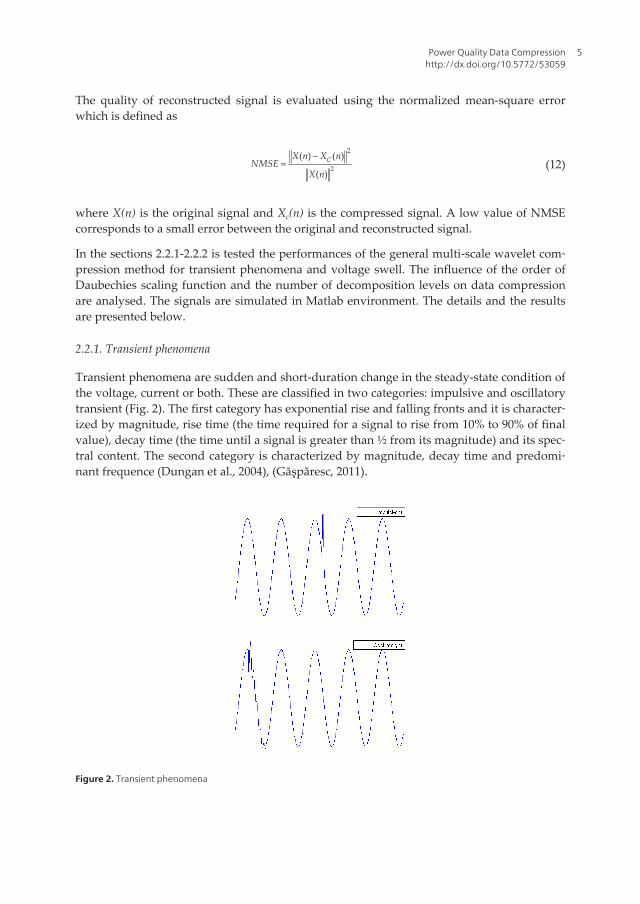
Transient phenomena are sudden and short-duration change in the steady-state condition ofthe voltage, current or both. These are classified in two categories: impulsive and oscillatorytransient (Fig. 2). The first category has exponential rise and falling fronts and it is character‐ized by magnitude, rise time (the time required for a signal to rise from 10% to 90% of finalvalue), decay time (the time until a signal is greater than ½ from its magnitude) and its spec‐tral content. The second category is characterized by magnitude, decay time and predomi‐nant frequence (Dungan et al., 2004), (Găşpăresc, 2011).

Figure 2. Transient phenomena


5

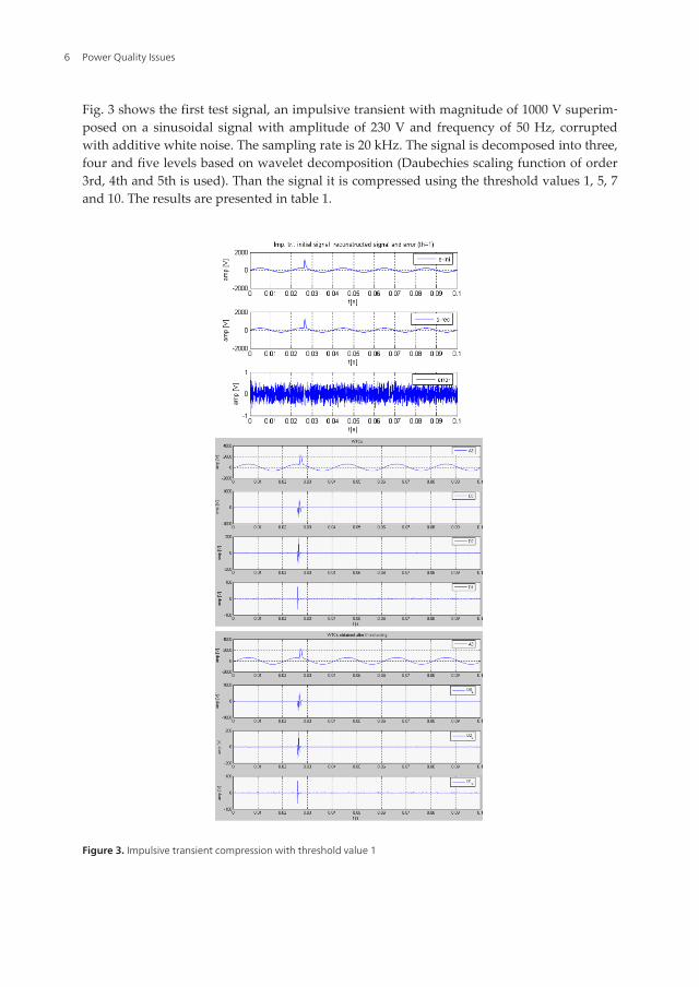
Fig. 3 shows the first test signal, an impulsive transient with magnitude of 1000 V superim‐posed on a sinusoidal signal with amplitude of 230 V and frequency of 50 Hz, corruptedwith additive white noise. The sampling rate is 20 kHz. The signal is decomposed into three,four and five levels based on wavelet decomposition (Daubechies scaling function of order3rd, 4th and 5th is used). Than the signal it is compressed using the threshold values 1, 5, 7and 10. The results are presented in table 1.

Figure 3. Impulsive transient compression with threshold value 1


Signal Ψ(t) Levels ηS NMSE [%] CR

Impulsive

transient

Db3 3 1 5.5154e-006 1.47

Db3 3 5 2.7151e-005 6.54

Db3 3 7 2.7827e-005 7.09

Db3 3 10 2.6502e-005 7.14

Db3 4 5 2.9240e-005 10.7

Db3 4 7 3.1081e-005 11.17

Db3 4 10 3.1515e-005 11.7

Db3 5 5 3.6143e-005 9.66

Db3 5 7 4.0148e-005 12.42

Db3 5 10 5.6165e-005 15.04

Db4 3 5 2.9386e-005 6.94

Db4 3 7 2.9246e-005 7.14

Db4 3 10 2.9481e-005 7.3

Db4 4 5 3.2845e-005 10.47

Db4 4 7 3.0742e-005 10.93

Db4 4 10 3.1029e-005 11.05

Db5 4 5 3.0875e-005 9.85

Db5 4 7 2.8626e-005 10.36

Db5 4 10 3.1029e-005 10.69

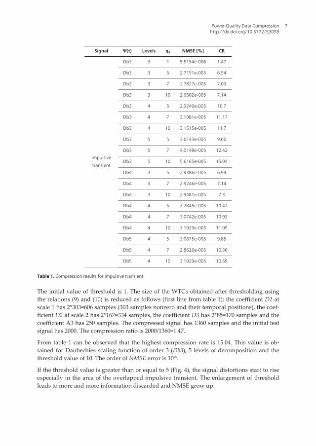
Table 1. Compression results for impulsive transient

The initial value of threshold is 1. The size of the WTCs obtained after thresholding usingthe relations (9) and (10) is reduced as follows (first line from table 1): the coefficient D1 atscale 1 has 2*303=606 samples (303 samples nonzero and their temporal positions), the coef‐ficient D2 at scale 2 has 2*167=334 samples, the coefficient D3 has 2*85=170 samples and thecoefficient A3 has 250 samples. The compressed signal has 1360 samples and the initial testsignal has 2000. The compression ratio is 2000/1360=1.47.

From table 1 can be observed that the highest compression rate is 15.04. This value is ob‐tained for Daubechies scaling function of order 3 (Db3), 5 levels of decomposition and thethreshold value of 10. The order of NMSE error is 10-6.

If the threshold value is greater than or equal to 5 (Fig. 4), the signal distortions start to riseespecially in the area of the overlapped impulsive transient. The enlargement of thresholdleads to more and more information discarded and NMSE grow up.


7

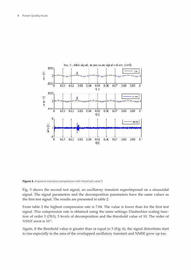
Figure 4. Impulsive transient compression with threshold value 5

Fig. 5 shows the second test signal, an oscillatory transient superimposed on a sinusoidalsignal. The signal parameters and the decomposition parameters have the same values asthe first test signal. The results are presented in table 2.

From table 2 the highest compression rate is 7.84. The value is lower than for the first testsignal. This compression rate is obtained using the same settings: Daubechies scaling func‐tion of order 3 (Db3), 5 levels of decomposition and the threshold value of 10. The order ofNMSE error is 10-5.

Again, if the threshold value is greater than or equal to 5 (Fig. 6), the signal distortions startto rise especially in the area of the overlapped oscillatory transient and NMSE grow up too.


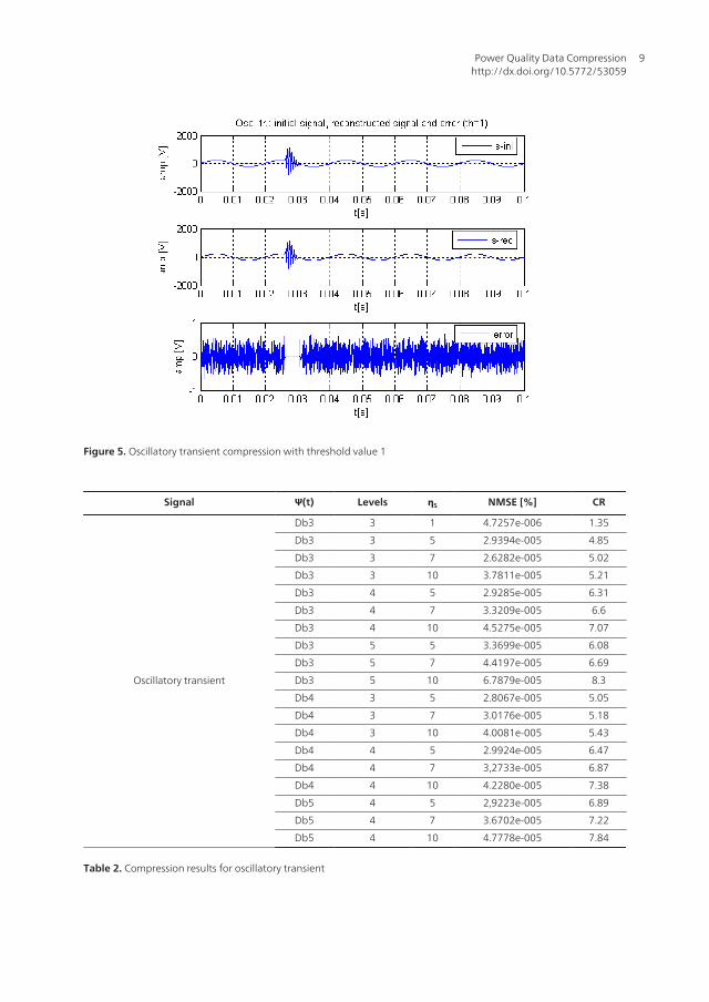
Figure 5. Oscillatory transient compression with threshold value 1


Oscillatory transient

Db3 3 1 4.7257e-006 1.35

Db3 3 5 2.9394e-005 4.85

Db3 3 7 2.6282e-005 5.02

Db3 3 10 3.7811e-005 5.21

Db3 4 5 2.9285e-005 6.31

Db3 4 7 3.3209e-005 6.6

Db3 4 10 4.5275e-005 7.07

Db3 5 5 3.3699e-005 6.08

Db3 5 7 4.4197e-005 6.69

Db3 5 10 6.7879e-005 8.3

Db4 3 5 2.8067e-005 5.05

Db4 3 7 3.0176e-005 5.18

Db4 3 10 4.0081e-005 5.43

Db4 4 5 2.9924e-005 6.47

Db4 4 7 3,2733e-005 6.87

Db4 4 10 4.2280e-005 7.38

Db5 4 5 2,9223e-005 6.89

Db5 4 7 3.6702e-005 7.22

Db5 4 10 4.7778e-005 7.84

Table 2. Compression results for oscillatory transient


9

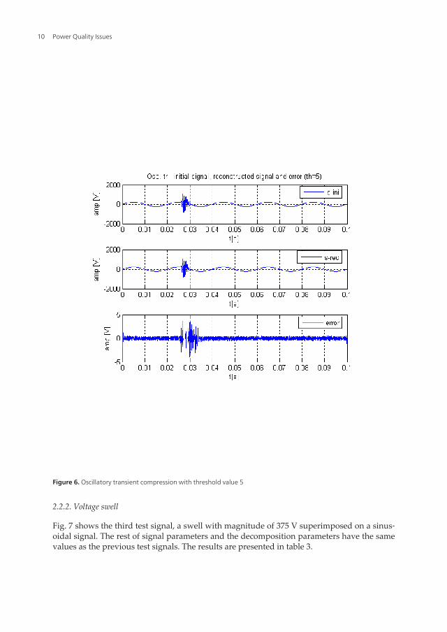
Figure 6. Oscillatory transient compression with threshold value 5

2.2.2. Voltage swell

Fig. 7 shows the third test signal, a swell with magnitude of 375 V superimposed on a sinus‐oidal signal. The rest of signal parameters and the decomposition parameters have the samevalues as the previous test signals. The results are presented in table 3.


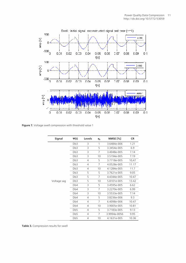
Figure 7. Voltage swell compression with threshold value 1


Voltage sag

Db3 3 1 3.6484e-006 1.21Db3 3 5 3.3454e-005 6.9Db3 3 7 3.4048e-005 7.14Db3 3 10 3.5194e-005 7.19Db3 4 5 3.7718e-005 10,47Db3 4 7 4.0528e-005 11.17Db3 4 10 4.1284e-005 11.7Db3 5 5 3.7621e-005 9.05Db3 5 7 4.4344e-005 10.47Db3 5 10 5.8101e-005 13.42Db4 3 5 3.4595e-005 6.62Db4 3 7 3.2270e-005 6.99Db4 3 10 3.5533e-005 7.14Db4 4 5 3.8236e-006 9.3Db4 4 7 6.4098e-006 10.47Db4 4 10 3.9005e-005 10.81Db5 4 5 3.7183e-005 9.13Db5 4 7 3.9994e-0056 9.95Db5 4 10 4.1631e-005 10.36

Table 3. Compression results for swell


11

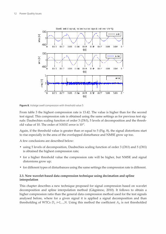
Figure 8. Volatge swell compression with threshold value 5

From table 3 the highest compression rate is 13.42. The value is higher than for the secondtest signal. This compression rate is obtained using the same settings as for previous test sig‐nals: Daubechies scaling function of order 3 (Db3), 5 levels of decomposition and the thresh‐old value of 10. The order of NMSE error is 10-5.

Again, if the threshold value is greater than or equal to 5 (Fig. 8), the signal distortions startto rise especially in the area of the overlapped disturbance and NMSE grow up too.

A few conclusions are described below:

• using 5 levels of decomposition, Daubechies scaling function of order 3 (Db3) and 5 (Db5)is obtained the highest compression rate;

• for a higher threshold value the compression rate will be higher, but NMSE and signaldistorsions grow up;

• for different types of disturbances using the same settings the compression rate is different.

2.3. New wavelet-based data compression technique using decimation and splineinterpolation

This chapter describes a new technique proposed for signal compression based on waveletdecomposition and spline interpolation method (Găşpăresc, 2010). It follows to obtain ahigher compression ratio than the general data compression method used for the test signalsanalysed before, where for a given signal it is applied a signal decomposition and thanthresholding of WTCs Di, i=1,...,N. Using this method the coefficient AN is not thresholded


and it has the largest number of samples from all the coefficients of signal decomposition. Inorder to obtain a higher sample rate this coefficient is decimated with a decimation factor Fdand at signal reconstruction will be interpolated. The cost is the increase of NMSE error.

Given an interval [a,b] and a divizion ∆:a=x0<x1<...<xn=b, a function S : [a,b]→R is called cubicspline interpolation function if this function meets the next conditions:

• S is a polynomial of degree at most 3 on any interval (xk,xk+1), k=1,…,N (relation 13);

• SєC2([a,b]);

• S(xi)=f(xi), iє(o,1,..., n), where f(x) is the interpolated function.

2 31( ) , [ , ]i i i i i iS x a b x c x d x x x x-= + + + " Î (13)

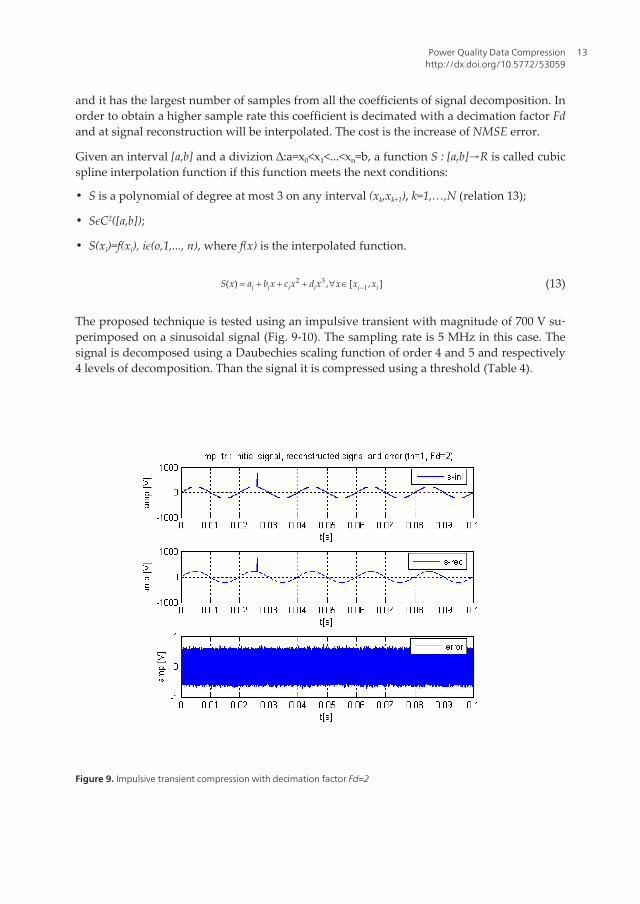
The proposed technique is tested using an impulsive transient with magnitude of 700 V su‐perimposed on a sinusoidal signal (Fig. 9-10). The sampling rate is 5 MHz in this case. Thesignal is decomposed using a Daubechies scaling function of order 4 and 5 and respectively4 levels of decomposition. Than the signal it is compressed using a threshold (Table 4).

Figure 9. Impulsive transient compression with decimation factor Fd=2


13

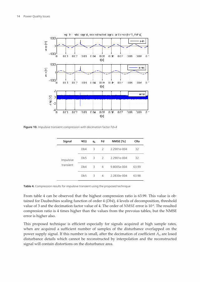
Figure 10. Impulsive transient compression with decimation factor Fd=4

Signal Ψ(t) ηS Fd NMSE [%] CRa

Impulsive

transient

Db4 3 2 2.2901e-004 32

Db5 3 2 2.2901e-004 32

Db4 3 4 9.8005e-004 63.99

Db5 3 4 2.2830e-004 63.98

Table 4. Compression results for impulsive transient using the proposed technique

From table 4 can be observed that the highest compression ratio is 63.99. This value is ob‐tained for Daubechies scaling function of order 4 (Db4), 4 levels of decomposition, thresholdvalue of 3 and the decimation factor value of 4. The order of NMSE error is 10-4. The resultedcompresion ratio is 4 times higher than the values from the prevoius tables, but the NMSEerror is higher also.

This proposed technique is efficient especially for signals acquired at high sample rates,when are acquired a sufficient number of samples of the disturbance overlapped on thepower supply signal. If this number is small, after the decimation of coefficient AN are loseddisturbance details which cannot be reconstructed by interpolation and the reconstructedsignal will contain distortions on the disturbance area.


3. Data compression using slantlet transform

3.1. Slantlet transform

The Slantlet transform (SLT) is a relatively new multiresolution technique base on DWT. Infact, it is an orthogonal DWT with two zero moments and compared to DWT provides bettertime localization (Selesnick, 1999), (Panda et al., 2002), (Duda, 2008).

In (Panda et al., 2002) is proposed a new approach for power quality data compressionbased on SLT. The technique is compared with the discrete cosine transform (DCT) and thediscrete wavelet transform (DWT) using various types of power quality disturbances (im‐pulse, sag, swell, harmonics, momentary interruption, oscillatory transient, voltage flicker).

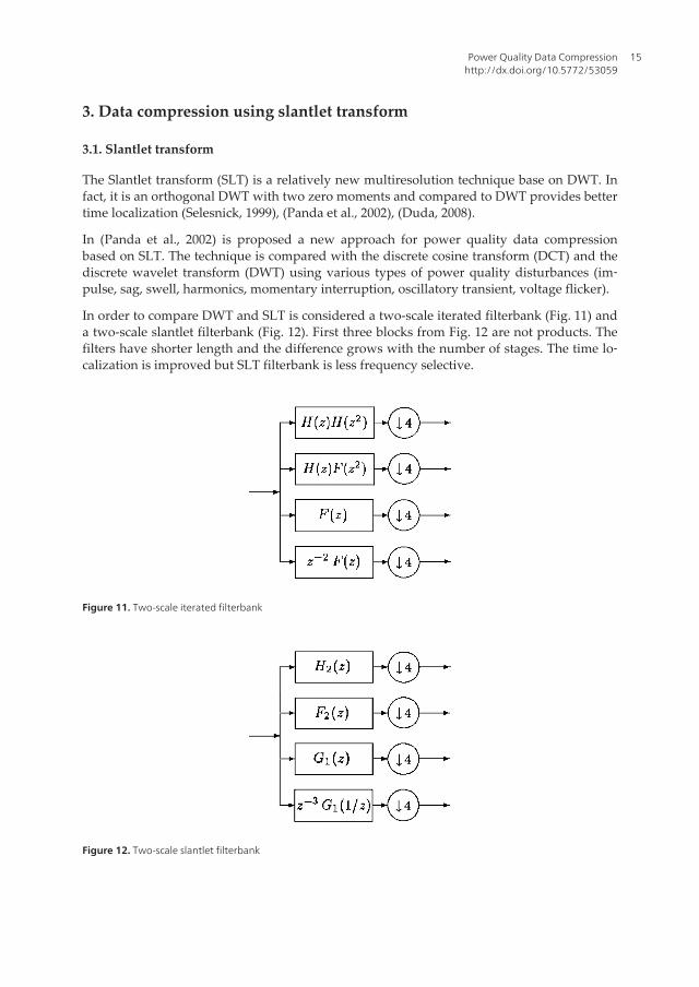
In order to compare DWT and SLT is considered a two-scale iterated filterbank (Fig. 11) anda two-scale slantlet filterbank (Fig. 12). First three blocks from Fig. 12 are not products. Thefilters have shorter length and the difference grows with the number of stages. The time lo‐calization is improved but SLT filterbank is less frequency selective.

Figure 11. Two-scale iterated filterbank

Figure 12. Two-scale slantlet filterbank


15

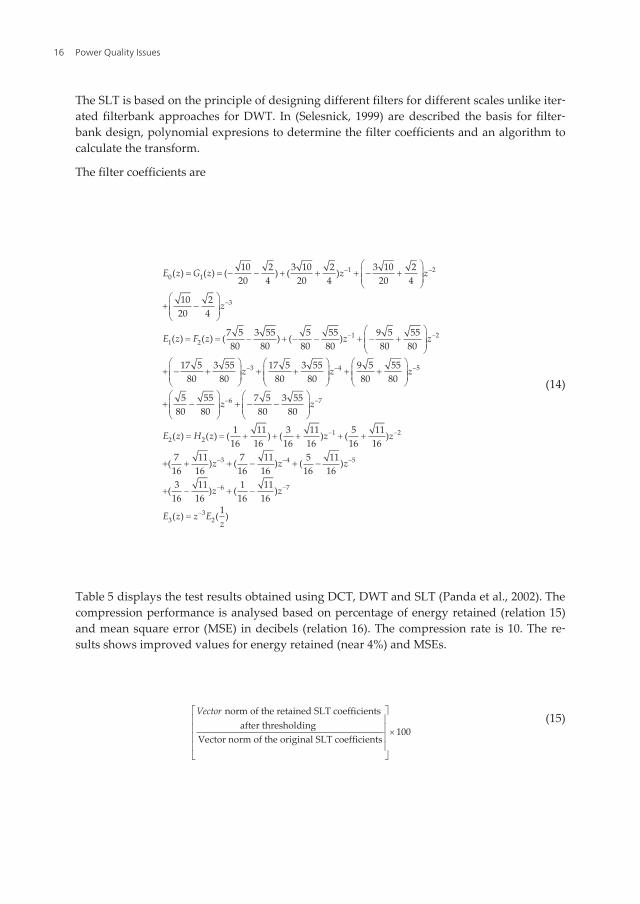
The SLT is based on the principle of designing different filters for different scales unlike iter‐ated filterbank approaches for DWT. In (Selesnick, 1999) are described the basis for filter‐bank design, polynomial expresions to determine the filter coefficients and an algorithm tocalculate the transform.

The filter coefficients are

1 20 1

3

1 21 2

3 4

10 2 3 10 2 3 10 2( ) ( ) ( ) ( )20 4 20 4 20 4

10 220 4

7 5 3 55 5 55 9 5 55( ) ( ) ( ) ( )80 80 80 80 80 80

17 5 3 55 17 5 3 55 9 5 5580 80 80 80 80 80

E z G z z z

z

E z F z z z

z z

- -

-

- -

- -

æ ö= = - - + + + - +ç ÷ç ÷

è øæ ö

+ -ç ÷ç ÷è ø

æ ö= = - + - - + - +ç ÷ç ÷

è øæ ö æ ö æ ö

+ - + + + + +ç ÷ ç ÷ çç ÷ ç ÷ çè ø è ø è ø

5

6 7

1 22 2

3 4 5

6 7

33 2

5 55 7 5 3 5580 80 80 80

1 11 3 11 5 11( ) ( ) ( ) ( ) ( )16 16 16 16 16 16

7 11 7 11 5 11( ) ( ) ( )16 16 16 16 16 163 11 1 11( ) ( )

16 16 16 161( ) ( )

z

z z

E z H z z z

z z z

z z

E z z Ez

-

- -

- -

- - -

- -

-

÷÷

æ ö æ ö+ - + - -ç ÷ ç ÷ç ÷ ç ÷è ø è ø

= = + + + + +

+ + + - + -

+ - + -

=

(14)

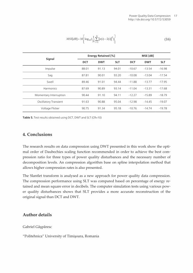
Table 5 displays the test results obtained using DCT, DWT and SLT (Panda et al., 2002). Thecompression performance is analysed based on percentage of energy retained (relation 15)and mean square error (MSE) in decibels (relation 16). The compression rate is 10. The re‐sults shows improved values for energy retained (near 4%) and MSEs.

norm of the retained SLT coefficients after thresholding 100Vector norm of the original SLT coefficients

Vectoré ùê úê ú ´ê úê úë û

(15)


210

1

1 ˆ[ ] 10 log ( ( ) ( ) )N

iMSE dB x i x i

N =

é ù= -ê ú

ê úë ûå (16)

SignalEnergy Retained [%] MSE [dB]

DCT DWT SLT DCT DWT SLT

Impulse 88.01 91.13 94.01 -10.67 -13.54 -16.98

Sag 87.81 90.01 93.20 -10.08 -13.04 -17.54

Swell 89.46 91.01 94.44 -11.88 -13.77 -17.95

Harmonics 87.69 90.89 93.14 -11.04 -13.31 -17.68

Momentary Interruption 90.44 91.10 94.11 -12.27 -15.89 -18.79

Oscillatory Transient 91.63 90.88 95.04 -12.98 -14.45 -19.07

Voltage Flicker 90.75 91.34 95.18 -10.76 -14.74 -19.78

Table 5. Test results obtained using DCT, DWT and SLT (CR=10)

4. Conclusions

The research results on data compression using DWT presented in this work show the opti‐mal order of Daubechies scaling function recommended in order to achieve the best com‐pression ratio for three types of power quality disturbances and the necessary number ofdecomposition levels. An compression algorithm base on spline interpolation method thatallows higher compression rates is also presented.

The Slantlet transform is analysed as a new approach for power quality data compression.The compression performance using SLT was compared based on percentage of energy re‐tained and mean square error in decibels. The computer simulation tests using various pow‐er quality disturbances shows that SLT provides a more accurate reconstruction of theoriginal signal than DCT and DWT.

Author details

Gabriel Găşpăresc

“Politehnica” University of Timişoara, Romania


17

References

[1] Azam, M. S. ., Tu, F. ., Pattipati, K. R. ., & Karanam, R. (2004). A Dependency ModelBased Approach for Identifying and Evaluating Power Quality Problems, IEEETransactions on Power Delivery 19(3), , 1154-1166.

[2] Barrera, Nunez. V. ., Melendez, Frigola. J. ., & Herraiz, Jaramillo. S. (2008). A Surveyon Voltage Dip Events in Power Systems, Proceedings of the International Confer‐ence on Renewable Energies and Power Quality.

[3] Bollen, M. ., & Gu, I. (2006). Signal Processing of Power Quality Disturbances. JohnWiley & Sons.

[4] Dash, P. K. ., Nayak, M. ., Senapati, M. R., & Lee, I. W. C. (2007). Mining for similari‐ties in time series data using wavelet-based feature vectors and neural networks. En‐gineering Applications of Artificial Intelligence, 185-201.

[5] Duda, K. (2008). Lifting Based Compression Algorithm for Power Systems Signals,Metrology and Measurement Systems XV(1), , 69-83.

[6] Dungan, R. C. ., Mc Granaghan, M. F. ., Santoso, S. ., & Beaty, H. W. (2004). ElectricalPower System Quality, McGraw-Hill.

[7] Găşpăresc, G. (2010). Data compression of power quality disturbances using wavelettransform and spline interpolation method, Proceedings of the 9th International Con‐ference on Environment and Electrical Engineering.

[8] Găşpăresc, G. (2011). Methodes of Power Quality Analysis, in Power Quality- Moni‐toring, Analysis and Enhancement, Ed. Ahmed Zobaa, Mario Manana Canteli andRamesh Bansal, Chapter 6, INTECH., 101-118.

[9] Hamid, E. Y. ., & Kawasasaki, Z. I. (2002). Wavelet-based data compression of powerdisturbances using the minimum description length criterion, IEEE. Transactions onPower Delivery 17, , 460-466.

[10] Lin, L. ., Huang, N. ., & Huang, W. (2009). Review of Power Quality Signal Compres‐sion Based on Wavelet Theory. Proceedings of the International Conference on Testand Measurement.

[11] Littler, T. B. ., & Morrow, D. J. (1999). Wavelets for the analysis and compression ofpower system disturbances. IEEE Transactions on Power Delivery 14, , 358-364.

[12] Lorio, F. ., & Magnago, F. (2004). Analysis of Data Compression Methods for PowerQualiy Events, Proceedings of the Power Engineering Society General Meeting.

[13] Qian, S. (2002). Time-Frequency and Wavelet Transforms, Prentice Hall PTR.


[14] Panda, G. ., Dash, P. K., Pradhan, A. K., & Meher, S. K. (2002). Data Compression ofPower Qualtity Events Using the Slantlet Transform, IEEE Transactions on PowerDelivery 17(2), , 662-667.

[15] Ribeiro, M. V. ., Park, S. H. ., Romano, J. M. T. ., & Duque, C. A. (2004). An ImprovedMethod for Signal Processing and Compression in Power Quality Evaluation. IEEETransactions on Power Delivery, 464-471.

[16] Ribeiro, M. V. ., Park, S. H. ., Romano, J. M. T. ., & Mitra, S. K. (2007). A Novel MDL-based Compression Method for Power Quality Applications. IEEE Transactions onPower Delivery 22(1), , 27-36.

[17] Santoso, S. ., Powers, E. J. ., & Grady, W. M. (1997). Power Quality Disturbance DataCompression using Wavelet Transform Methods. IEEE Transactions on Power Deliv‐ery 12(3), , 1250-1256.

[18] Selesnick, I. W. (1999). The Slantlet Transform. IEEE Transactions on Signal Processing,1304-1313.

[19] Zhang, M. ., Li, K. ., & Hu, Y. (2011). A High Efficient Compression Method for Pow‐er Quality Applications, IEEE Transaction on Power Delivery 60(6), , 1976-1985.

[20] Wang, J. ., & Wang, C. (2005). Compression of Power Quality Disturbance DataBased on Energy and Adaptive Arithmetic Encoding, Proceedings of the TENCON.

[21] Wu, C. J. ., & Fu, T. H. (2003). Data compression applied to electric power qualitytracking of arc furnance load, Journal of Marine Science and Technology 11, , 39-47.


19

Documents

Power Quality Data Compression - InTech - Opencdn.intechopen.com/pdfs/44193/InTech-Power_quality... · Power Quality Data Compression ... A D D A D D D = + = + + = + + + (8) The decomposition