Predicting Abnormal Returns From News Using Text Classification

Ronny Luss∗ Alexandre d’Aspremont†

August 2, 2009

Abstract

We show how text from news articles can be used to predict intraday price movements of financial as-sets using support vector machines. Multiple kernel learning is used to combine equity returns with textas predictive features in order to increase classification performance and we develop an analytic centercutting plane method to solve the kernel learning problem efficiently. This method exhibits linear con-vergence but requires very few gradient evaluations (each of them a support vector machine classificationproblem), making it particularly efficient on the large sample sizes considered in this application.

1 Introduction

Asset pricing models often describe the arrival of novel information by a jump process, but the characteristicsof the underlying jump process are only coarsely, if at all, related to the underlying source of information.Similarly, time series models such as ARCH and GARCH have been developed to forecast volatility usingasset returns data but these methods also ignore one key source of market volatility: financial news. Ourobjective here is to show that text classification techniques allow a much more refined analysis of the impactof news on asset prices.

Empirical studies that examine stock return predictability can be traced back to Fama (1965) amongothers, who showed that there is no significant autocorrelation in the daily returns of thirty stocks from theDow-Jones Industrial Average. Similar studies were conducted by Taylor (1986) and Ding et al. (1993),who find significant autocorrelation in squared and absolutereturns (i.e. volatility). These effects are alsoobserved on intraday volatility patterns as demonstrated by Wood et al. (1985) and by Andersen & Bollerslev(1997) on absolute returns. These findings tend to demonstrate that, given solely historical stock returns,stock returns are not predictable while volatility is. The impact of news articles has also been studiedextensively. Ederington & Lee (1993) for example studied price fluctuations in interest rate and foreignexchange futures markets following macroeconomic announcements and showed that prices mostly adjustedwithin one minute of major announcements. Mitchell & Mulherin (1994) aggregated daily announcementsby Dow Jones & Companyinto a single variable and found no correlation with market absolute returns andweak correlation with firm-specific absolute returns. However, Kalev et al. (2004) aggregated intraday newsconcerning companies listed on the Australian Stock Exchange into an exogenous variable in a GARCHmodel and found significant predictive power. These findingsare attributed to the conditioning of volatilityon news. Results were further improved by restricting the type of news articles included.

∗ORFE Department, Princeton University, Princeton, NJ 08544. rluss@princeton.edu†ORFE Department, Princeton University, Princeton, NJ 08544. aspremon@princeton.edu

1

The most common techniques for forecasting volatility are often based on Autoregressive ConditionalHeteroskedasticity (ARCH) and Generalized ARCH (GARCH) models mentioned above. For example,intraday volatility in foreign exchange and equity marketsis modeled with MA-GARCH in Andersen &Bollerslev (1997) and ARCH in Taylor & Xu (1997). See Bollerslev et al. (1992) for a survey of ARCH andGARCH models and various other applications. Machine learning techniques such as neural networks andsupport vector machines have also been used to forecast volatility. Neural networks are used in Malliaris& Salchenberger (1996) to forecast implied volatility of options on the SP100 index, and support vectormachines are used to forecast volatility of the SP500 index using daily returns in Gavrishchaka & Banerjee(2006).

Here, we show that information from press releases can be used to predict intraday abnormal returnswith relatively high accuracy. Consistent with Taylor (1986) and Ding et al. (1993), however, the directionof returns is not found to be predictable. We form a text classification problem where press releases arelabeled positive if the absolute return jumps at some (fixed)time after the news is made public. Supportvector machines (SVM) are used to solve this classification problem using both equity returns and wordfrequencies from press releases. Furthermore, we use multiple kernel learning (MKL) to optimally combineequity returns with text as predictive features and increase classification performance.

Text classification is a well-studied problem in machine learning, (Dumais et al. (1998) and Joachims(2002) among many others show that SVM significantly outperform classic methods such as naive bayes).Initially, naive bayes classifiers were used in Wuthrich et al. (1998) to do three-class classification of anindex using daily returns for labels. News is taken from several sources such asReutersand The WallStreet Journal. Five-class classification with naive bayes classifiers is used in Lavrenko et al. (2000) toclassify intraday price trends when articles are publishedat theYAHOO!Financewebsite. Support vectormachines were also used to classify intraday price trends inFung et al. (2003) usingReutersarticles and inM.-A.Mittermayer & Knolmayer (2006a) to do four-class classification of stock returns using press releasesby PRNewswire. Text classification has also been used to directly predict volatility (see M.-A.Mittermayer& Knolmayer (2006b) for a survey of trading systems that use text). Recently, Robertson et al. (2007) usedSVM to predict if articles from theBloomberg serviceare followed by abnormally large volatility; articlesdeemed important are then aggregated into a variable and used in a GARCH model similar to Kalev et al.(2004). ? use Support Vector Regression (SVR) to forecast stock return volatility based on text in SECmandated 10-K reports. They found that reports published after the Sarbanes-Oxley Act of 2002 improvedforecasts over baseline methods that did not use text. Generating trading rules with genetic programming(GP) is another way to incorporate text for financial tradingsystems. Trading rules are created in Dempster& Jones (2001) using GP for foreign exchange markets based ontechnical indicators and extended in Austinet al. (2004) to combine technical indicators with non-publicly available information. Ensemble methodswere used in Thomas (2003) on top of GP to create rules based onheadlines posted onYahoointernetmessage boards.

Our contribution here is twofold. First, abnormal returns are predicted using text classification tech-niques similar to M.-A.Mittermayer & Knolmayer (2006a). Given a press release, we predict whether ornot an abnormal return will occur in the next10, 20, ..., 250 minutes using text and past absolute returns.The algorithm in M.-A.Mittermayer & Knolmayer (2006a) uses text to predict whether returns jump up 3%,down 3%, remain within these bounds, or are “unclear” within15 minutes of a press release. They considera nine months subset of the eight years of press releases usedhere. Our experiments analyze predictabilityof absolute returns at many horizons and demonstrate significant initial intraday predictability that decreasesthroughout the trading day. Second, we optimally combine text information with asset price time series tosignificantly enhance classification performance using multiple kernel learning (MKL). We use an analytic

2

center cutting plane method (ACCPM) to solve the resulting MKL problem. ACCPM is particularly efficienton problems where the objective function and gradient are hard to evaluate but whose feasible set is simpleenough so that analytic centers can be computed efficiently.Furthermore, because it does not suffer fromconditioning issues, ACCPM can achieve higher precision targets than other first-order methods.

The rest of the paper is organized as follows. Section 2 details the text classification problem we solvehere and provides predictability results using using either text or absolute returns as features. Section 3describes the multiple kernel learning framework and details the analytic center cutting plane algorithm usedto solve the resulting optimization problem. Finally, we use MKL to enhance the prediction performance.

2 Predictions with support vector machines

Here, we describe how support vector machines can be used to make binary predictions on equity returns.The experimental setup follows with results that use text and stock return data separately to make predictions.

2.1 Support vector machines

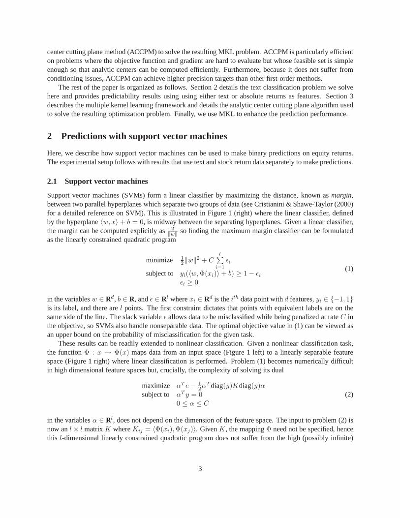
Support vector machines (SVMs) form a linear classifier by maximizing the distance, known asmargin,between two parallel hyperplanes which separate two groupsof data (see Cristianini & Shawe-Taylor (2000)for a detailed reference on SVM). This is illustrated in Figure 1 (right) where the linear classifier, definedby the hyperplane〈w, x〉 + b = 0, is midway between the separating hyperplanes. Given a linear classifier,the margin can be computed explicitly as2‖w‖ so finding the maximum margin classifier can be formulatedas the linearly constrained quadratic program

minimize 12‖w‖2 + C

l∑i=1

ǫi

subject to yi(〈w,Φ(xi)〉 + b) ≥ 1 − ǫi

ǫi ≥ 0

(1)

in the variablesw ∈ Rd, b ∈ R, andǫ ∈ Rl wherexi ∈ Rd is theith data point withd features,yi ∈ {−1, 1}is its label, and there arel points. The first constraint dictates that points with equivalent labels are on thesame side of the line. The slack variableǫ allows data to be misclassified while being penalized at rateC inthe objective, so SVMs also handle nonseparable data. The optimal objective value in (1) can be viewed asan upper bound on the probability of misclassification for the given task.

These results can be readily extended to nonlinear classification. Given a nonlinear classification task,the functionΦ : x → Φ(x) maps data from an input space (Figure 1 left) to a linearly separable featurespace (Figure 1 right) where linear classification is performed. Problem (1) becomes numerically difficultin high dimensional feature spaces but, crucially, the complexity of solving its dual

maximize αT e − 12αT diag(y)Kdiag(y)α

subject to αT y = 00 ≤ α ≤ C

(2)

in the variablesα ∈ Rl, does not depend on the dimension of the feature space. The input to problem (2) isnow anl × l matrixK whereKij = 〈Φ(xi),Φ(xj)〉. GivenK, the mappingΦ need not be specified, hencethis l-dimensional linearly constrained quadratic program doesnot suffer from the high (possibly infinite)

3

5 10 1511.5

12

12.5

13

13.5

14

14.5

15

15.5

5 6 7 8 9 10 11 12 13 14 1516

18

20

22

24

26

28

30

32

34

36

2 / ||w||

<w,x> + b = −1

<w,x> + b = +1

Figure 1: Input Space vs. Feature Space. For nonlinear classification, data is mapped from the inputspace to the feature space. Linear classification is performed by support vector machines on mappeddata in the feature space.

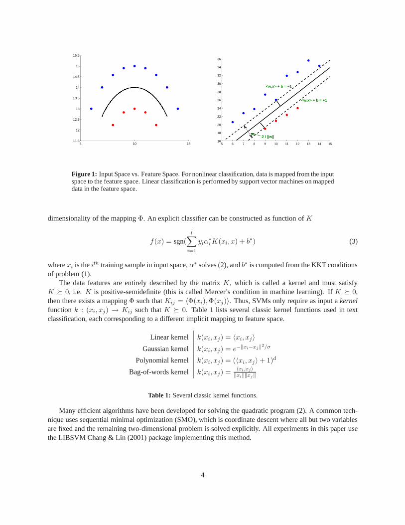
dimensionality of the mappingΦ. An explicit classifier can be constructed as function ofK

f(x) = sgn(l∑

i=1

yiα∗i K(xi, x) + b∗) (3)

wherexi is theith training sample in input space,α∗ solves (2), andb∗ is computed from the KKT conditionsof problem (1).

The data features are entirely described by the matrixK, which is called a kernel and must satisfyK � 0, i.e. K is positive-semidefinite (this is called Mercer’s condition in machine learning). IfK � 0,then there exists a mappingΦ such thatKij = 〈Φ(xi),Φ(xj)〉. Thus, SVMs only require as input akernelfunction k : (xi, xj) → Kij such thatK � 0. Table 1 lists several classic kernel functions used in textclassification, each corresponding to a different implicitmapping to feature space.

Linear kernel k(xi, xj) = 〈xi, xj〉Gaussian kernel k(xi, xj) = e−‖xi−xj‖

2/σ

Polynomial kernel k(xi, xj) = (〈xi, xj〉 + 1)d

Bag-of-words kernel k(xi, xj) =〈xi,xj〉‖xi‖‖xj‖

Table 1: Several classic kernel functions.

Many efficient algorithms have been developed for solving the quadratic program (2). A common tech-nique uses sequential minimal optimization (SMO), which iscoordinate descent where all but two variablesare fixed and the remaining two-dimensional problem is solved explicitly. All experiments in this paper usethe LIBSVM Chang & Lin (2001) package implementing this method.

4

2.2 Data

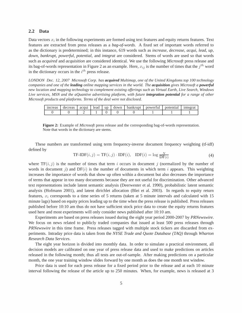
Data vectorsxi in the following experiments are formed using text featuresand equity returns features. Textfeatures are extracted from press releases as abag-of-words. A fixed set of important words referred toas the dictionary is predetermined; in this instance, 619 words such asincrease, decrease, acqui, lead, up,down, bankrupt, powerful, potential, and integrat are considered. Stems of words are used so that wordssuch asacquiredandacquisitionare considered identical. We use the followingMicrosoftpress release andits bag-of-words representation in Figure 2 as an example. Here,xij is the number of times that thejth wordin the dictionary occurs in theith press release.

LONDON Dec. 12, 2007 Microsoft Corp. hasacquired Multimap, one of the United Kingdoms top 100 technologycompanies and one of theleading online mapping services in the world. Theacquisition gives Microsoft apowerfulnew location and mapping technology to complement existingofferings such as Virtual Earth, Live Search, WindowsLive services, MSN and the aQuantive advertising platform,with future integration potential for a range of otherMicrosoft products and platforms. Terms of the deal were notdisclosed.

increas decreas acqui lead up down bankrupt powerful potential integrat0 0 2 1 0 0 0 1 1 1

Figure 2: Example ofMicrosoft press release and the corresponding bag-of-words representation.Note that words in the dictionary are stems.

These numbers are transformed using term frequency-inverse document frequency weighting (tf-idf)defined by

TF-IDF(i, j) = TF(i, j) · IDF(i), IDF(i) = log NDF(i) (4)

where TF(i, j) is the number of times that termi occurs in documentj (normalized by the number ofwords in documentj) and DF(i) is the number of documents in which termi appears. This weightingincreases the importance of words that show up often within adocument but also decreases the importanceof terms that appear in too many documents because they are not useful for discrimination. Other advancedtext representations include latent semantic analysis (Deerwester et al. 1990), probabilistic latent semanticanalysis (Hofmann 2001), and latent dirichlet allocation (Blei et al. 2003). In regards to equity returnfeatures,xi corresponds to a time series of 5 returns (taken at 5 minute intervals and calculated with 15minute lags) based on equity prices leading up to the time when the press release is published. Press releasespublished before 10:10 am thus do not have sufficient stock price data to create the equity returns featuresused here and most experiments will only consider news published after 10:10 am.

Experiments are based on press releases issued during the eight year period 2000-2007 byPRNewswire.We focus on news related to publicly traded companies that issued at least 500 press releases throughPRNewswirein this time frame. Press releases tagged with multiple stock tickers are discarded from ex-periments. Intraday price data is taken from theNYSE Trade and Quote Database (TAQ)throughWhartonResearch Data Services.

The eight year horizon is divided into monthly data. In orderto simulate a practical environment, alldecision models are calibrated on one year of press release data and used to make predictions on articlesreleased in the following month; thus all tests are out-of-sample. After making predictions on a particularmonth, the one year training window slides forward by one month as does the one month test window.

Price data is used for each press release for a fixed period prior to the release and at each 10 minuteinterval following the release of the article up to 250 minutes. When, for example, news is released at 3

5

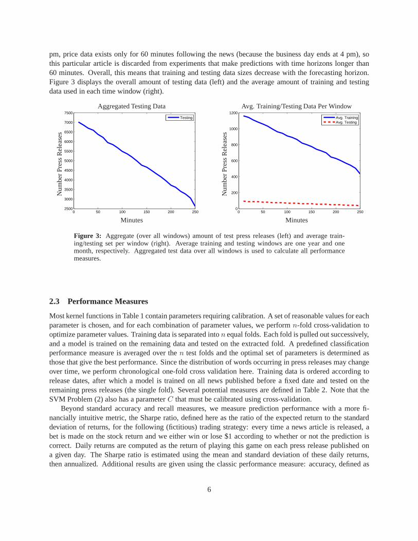
pm, price data exists only for 60 minutes following the news (because the business day ends at 4 pm), sothis particular article is discarded from experiments thatmake predictions with time horizons longer than60 minutes. Overall, this means that training and testing data sizes decrease with the forecasting horizon.Figure 3 displays the overall amount of testing data (left) and the average amount of training and testingdata used in each time window (right).

0 50 100 150 200 2502500

3000

3500

4000

4500

5000

5500

6000

6500

7000

7500

Testing

Aggregated Testing Data

Nu

mb

erP

ress

Rel

ease

s

Minutes0 50 100 150 200 250

0

200

400

600

800

1000

1200

Avg. TrainingAvg. Testing

Avg. Training/Testing Data Per Window

Nu

mb

erP

ress

Rel

ease

sMinutes

Figure 3: Aggregate (over all windows) amount of test press releases (left) and average train-ing/testing set per window (right). Average training and testing windows are one year and onemonth, respectively. Aggregated test data over all windowsis used to calculate all performancemeasures.

2.3 Performance Measures

Most kernel functions in Table 1 contain parameters requiring calibration. A set of reasonable values for eachparameter is chosen, and for each combination of parameter values, we performn-fold cross-validation tooptimize parameter values. Training data is separated inton equal folds. Each fold is pulled out successively,and a model is trained on the remaining data and tested on the extracted fold. A predefined classificationperformance measure is averaged over then test folds and the optimal set of parameters is determined asthose that give the best performance. Since the distribution of words occurring in press releases may changeover time, we perform chronological one-fold cross validation here. Training data is ordered according torelease dates, after which a model is trained on all news published before a fixed date and tested on theremaining press releases (the single fold). Several potential measures are defined in Table 2. Note that theSVM Problem (2) also has a parameterC that must be calibrated using cross-validation.

Beyond standard accuracy and recall measures, we measure prediction performance with a more fi-nancially intuitive metric, the Sharpe ratio, defined here as the ratio of the expected return to the standarddeviation of returns, for the following (fictitious) trading strategy: every time a news article is released, abet is made on the stock return and we either win or lose $1 according to whether or not the prediction iscorrect. Daily returns are computed as the return of playingthis game on each press release published ona given day. The Sharpe ratio is estimated using the mean and standard deviation of these daily returns,then annualized. Additional results are given using the classic performance measure: accuracy, defined as

6

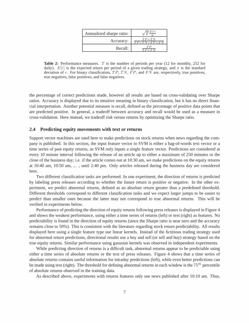
Annualized sharpe ratio:√

T E[r]σ

Accuracy: TP+TNTP+TN+FP+FN

Recall: TPTP+FN

Table 2: Performance measures.T is the number of periods per year (12 for monthly, 252 fordaily). E[r] is the expected return per period of a given trading strategy, andσ is the standarddeviation ofr. For binary classification,TP , TN , FP , andFN are, respectively, true positives,true negatives, false positives, and false negatives.

the percentage of correct predictions made, however all results are based on cross-validating over Sharperatios. Accuracy is displayed due to its intuitive meaning in binary classification, but it has no direct finan-cial interpretation. Another potential measure is recall,defined as the percentage of positive data points thatare predicted positive. In general, a tradeoff between accuracy and recall would be used as a measure incross-validation. Here instead, we tradeoff risk versus returns by optimizing the Sharpe ratio.

2.4 Predicting equity movements with text or returns

Support vector machines are used here to make predictions onstock returns when news regarding the com-pany is published. In this section, the input feature vectorto SVM is either a bag-of-words text vector or atime series of past equity returns, as SVM only inputs a single feature vector. Predictions are considered atevery 10 minute interval following the release of an articleup to either a maximum of 250 minutes or theclose of the business day; i.e. if the article comes out at 10:30 am, we make predictions on the equity returnsat 10:40 am, 10:50 am, ... , until 2:40 pm. Only articles released during the business day are consideredhere.

Two different classification tasks are performed. In one experiment, the direction of returns is predictedby labeling press releases according to whether the future return is positive or negative. In the other ex-periment, we predict abnormal returns, defined as an absolute return greater than a predefined threshold.Different thresholds correspond to different classification tasks and we expect larger jumps to be easier topredict than smaller ones because the latter may not correspond to true abnormal returns. This will beverified in experiments below.

Performance of predicting the direction of equity returns following press releases is displayed in Figure 4and shows the weakest performance, using either a time series of returns (left) or text (right) as features. Nopredictability is found in the direction of equity returns (since the Sharpe ratio is near zero and the accuracyremains close to 50%). This is consistent with the literature regarding stock return predictability. All resultsdisplayed here using a single feature type use linear kernels. Instead of the fictitious trading strategy usedfor abnormal return predictions, directional results use abuy and sell (or sell and buy) strategy based on thetrue equity returns. Similar performance using gaussian kernels was observed in independent experiments.

While predicting direction of returns is a difficult task, abnormal returns appear to be predictable usingeither a time series of absolute returns or the text of press releases. Figure 4 shows that a time series ofabsolute returns contains useful information for intradaypredictions (left), while even better predictions canbe made using text (right). The threshold for defining abnormal returns in each window is the75th percentileof absolute returns observed in the training data.

As described above, experiments with returns features onlyuse news published after 10:10 am. Thus,

7

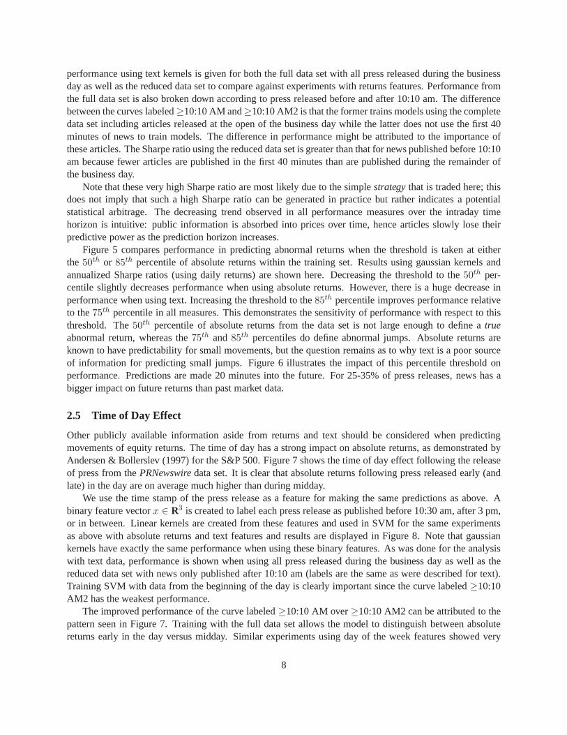
performance using text kernels is given for both the full data set with all press released during the businessday as well as the reduced data set to compare against experiments with returns features. Performance fromthe full data set is also broken down according to press released before and after 10:10 am. The differencebetween the curves labeled≥10:10 AM and≥10:10 AM2 is that the former trains models using the completedata set including articles released at the open of the business day while the latter does not use the first 40minutes of news to train models. The difference in performance might be attributed to the importance ofthese articles. The Sharpe ratio using the reduced data set is greater than that for news published before 10:10am because fewer articles are published in the first 40 minutes than are published during the remainder ofthe business day.

Note that these very high Sharpe ratio are most likely due to the simplestrategythat is traded here; thisdoes not imply that such a high Sharpe ratio can be generated in practice but rather indicates a potentialstatistical arbitrage. The decreasing trend observed in all performance measures over the intraday timehorizon is intuitive: public information is absorbed into prices over time, hence articles slowly lose theirpredictive power as the prediction horizon increases.

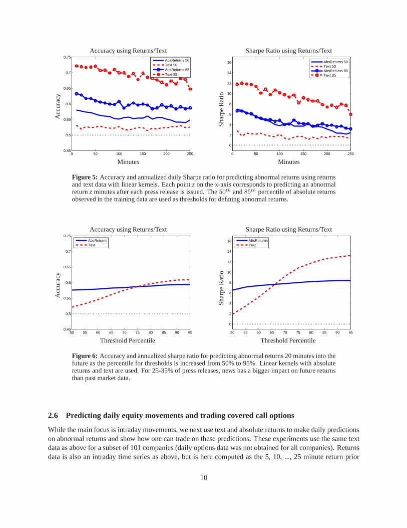
Figure 5 compares performance in predicting abnormal returns when the threshold is taken at eitherthe 50th or 85th percentile of absolute returns within the training set. Results using gaussian kernels andannualized Sharpe ratios (using daily returns) are shown here. Decreasing the threshold to the50th per-centile slightly decreases performance when using absolute returns. However, there is a huge decrease inperformance when using text. Increasing the threshold to the85th percentile improves performance relativeto the75th percentile in all measures. This demonstrates the sensitivity of performance with respect to thisthreshold. The50th percentile of absolute returns from the data set is not largeenough to define atrueabnormal return, whereas the75th and85th percentiles do define abnormal jumps. Absolute returns areknown to have predictability for small movements, but the question remains as to why text is a poor sourceof information for predicting small jumps. Figure 6 illustrates the impact of this percentile threshold onperformance. Predictions are made 20 minutes into the future. For 25-35% of press releases, news has abigger impact on future returns than past market data.

2.5 Time of Day Effect

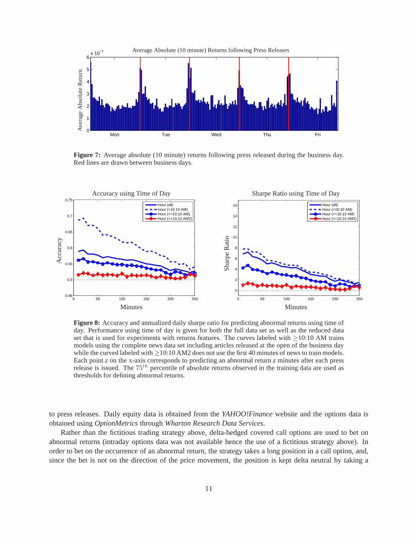
Other publicly available information aside from returns and text should be considered when predictingmovements of equity returns. The time of day has a strong impact on absolute returns, as demonstrated byAndersen & Bollerslev (1997) for the S&P 500. Figure 7 shows the time of day effect following the releaseof press from thePRNewswiredata set. It is clear that absolute returns following press released early (andlate) in the day are on average much higher than during midday.

We use the time stamp of the press release as a feature for making the same predictions as above. Abinary feature vectorx ∈ R3 is created to label each press release as published before 10:30 am, after 3 pm,or in between. Linear kernels are created from these features and used in SVM for the same experimentsas above with absolute returns and text features and resultsare displayed in Figure 8. Note that gaussiankernels have exactly the same performance when using these binary features. As was done for the analysiswith text data, performance is shown when using all press released during the business day as well as thereduced data set with news only published after 10:10 am (labels are the same as were described for text).Training SVM with data from the beginning of the day is clearly important since the curve labeled≥10:10AM2 has the weakest performance.

The improved performance of the curve labeled≥10:10 AM over≥10:10 AM2 can be attributed to thepattern seen in Figure 7. Training with the full data set allows the model to distinguish between absolutereturns early in the day versus midday. Similar experimentsusing day of the week features showed very

8

0 50 100 150 200 2500.45

0.5

0.55

0.6

0.65

0.7

0.75

AbsReturns AbnReturns Dir

Accuracy using ReturnsA

ccu

racy

Minutes0 50 100 150 200 250

0.45

0.5

0.55

0.6

0.65

0.7

0.75

Text Abn (all)Text Abn (<10:10 AM)Text Abn (>=10:10 AM)Text Abn (>=10:10 AM2)Text Dir (all)

Accuracy using Text

Acc

ura

cy

Minutes

0 50 100 150 200 250

0

2

4

6

8

10

12

14

16

AbsReturns AbnReturns Dir

Sharpe Ratio using Returns

Sh

arp

eR

atio

Minutes0 50 100 150 200 250

0

2

4

6

8

10

12

14

16

Text Abn (all)Text Abn (<10:10 AM)Text Abn (>=10:10 AM)Text Abn (>=10:10 AM2)Text Dir (all)

Sharpe Ratio using Text

Sh

arp

eR

atio

Minutes

Figure 4: Accuracy and annualized daily Sharpe ratio for predicting abnormal returns (Abn) ordirection of returns (Dir) using returns and text data with linear kernels. Performance using text isgiven for both the full data set as well as the reduced data setthat is used for experiments with returnsfeatures. The curves labeled with≥10:10 AM trains models using the complete data set includingarticles released at the open of the business day while the curved labeled with≥10:10 AM2 does notuse the first 40 minutes of news to train models. Each pointzon the x-axis corresponds to predictingan abnormal returnz minutes after each press release is issued. The75th percentile of absolutereturns observed in the training data is used as the threshold for defining an abnormal return.

weak performance and are thus not displayed. While the time of day effect exhibits predictability, notethat the experiments with text and absolute returns data do not use any time stamp features and henceperformance with text and absolute returns should not be attributed to any time of day effects. Furthermore,experiments below for combining the different pieces of publicly available information will show that thesetime of day effects are less useful than the text and returns data. There are of course other related marketmicrostructure effects that could be useful for predictability, such as the amount of news released throughoutthe day, etc.

9

0 50 100 150 200 2500.45

0.5

0.55

0.6

0.65

0.7

0.75

AbsReturns 50Text 50AbsReturns 85Text 85

Accuracy using Returns/TextA

ccu

racy

Minutes0 50 100 150 200 250

0

2

4

6

8

10

12

14

16

AbsReturns 50Text 50AbsReturns 85Text 85

Sharpe Ratio using Returns/Text

Sh

arp

eR

atio

Minutes

Figure 5: Accuracy and annualized daily Sharpe ratio for predicting abnormal returns using returnsand text data with linear kernels. Each pointz on the x-axis corresponds to predicting an abnormalreturnz minutes after each press release is issued. The50th and85th percentile of absolute returnsobserved in the training data are used as thresholds for defining abnormal returns.

50 55 60 65 70 75 80 85 90 950.45

0.5

0.55

0.6

0.65

0.7

0.75

AbsReturnsText

Accuracy using Returns/Text

Acc

ura

cy

Threshold Percentile50 55 60 65 70 75 80 85 90 95

0

2

4

6

8

10

12

14

16

AbsReturnsText

Sharpe Ratio using Returns/TextS

har

pe

Rat

io

Threshold Percentile

Figure 6: Accuracy and annualized sharpe ratio for predicting abnormal returns 20 minutes into thefuture as the percentile for thresholds is increased from 50% to 95%. Linear kernels with absolutereturns and text are used. For 25-35% of press releases, newshas a bigger impact on future returnsthan past market data.

2.6 Predicting daily equity movements and trading covered call options

While the main focus is intraday movements, we next use text and absolute returns to make daily predictionson abnormal returns and show how one can trade on these predictions. These experiments use the same textdata as above for a subset of 101 companies (daily options data was not obtained for all companies). Returnsdata is also an intraday time series as above, but is here computed as the 5, 10, ..., 25 minute return prior

10

Mon Tue Wed Thu Fri0

1

2

3

4

5

6x 10

−3 Average Absolute (10 minute) Returns following Press Releases

Ave

rage

Abs

olut

eR

etur

n

Figure 7: Average absolute (10 minute) returns following press released during the business day.Red lines are drawn between business days.

0 50 100 150 200 2500.45

0.5

0.55

0.6

0.65

0.7

0.75

Hour (all)Hour (<10:10 AM)Hour (>=10:10 AM)Hour (>=10:10 AM2)

Accuracy using Time of Day

Acc

ura

cy

Minutes0 50 100 150 200 250

0

2

4

6

8

10

12

14

16

Hour (all)Hour (<10:10 AM)Hour (>=10:10 AM)Hour (>=10:10 AM2)

Sharpe Ratio using Time of Day

Sh

arp

eR

atio

Minutes

Figure 8: Accuracy and annualized daily sharpe ratio for predicting abnormal returns using time ofday. Performance using time of day is given for both the full data set as well as the reduced dataset that is used for experiments with returns features. The curves labeled with≥10:10 AM trainsmodels using the complete news data set including articles released at the open of the business daywhile the curved labeled with≥10:10 AM2 does not use the first 40 minutes of news to train models.Each pointz on the x-axis corresponds to predicting an abnormal returnz minutes after each pressrelease is issued. The75th percentile of absolute returns observed in the training data are used asthresholds for defining abnormal returns.

to press releases. Daily equity data is obtained from theYAHOO!Financewebsite and the options data isobtained usingOptionMetricsthroughWharton Research Data Services.

Rather than the fictitious trading strategy above, delta-hedged covered call options are used to bet onabnormal returns (intraday options data was not available hence the use of a fictitious strategy above). Inorder to bet on the occurrence of an abnormal return, the strategy takes a long position in a call option, and,since the bet is not on the direction of the price movement, the position is kept delta neutral by taking a

11

short position in delta shares of stock (delta is defined as the change in call option price resulting from a$1 increase in stock price, here taken from theOptionMetricsdata). The position is exited the followingday by going short the call option and long delta shares of stock. A bet against an abnormal return takesthe opposite positions. Equity positions use the closing prices following the release of press and the closingprice the following day. Option prices (buy and sell) use an average of the best bid and ask price observedon the day of the press release. To normalize the size of positions, we always take a position in delta times$100 worth of the respective stock and the proper amount of the call option.

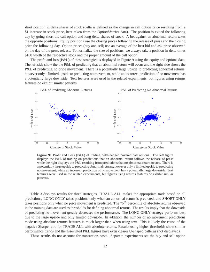
The profit and loss (P&L) of these strategies is displayed in Figure 9 using the equity and options data.The left side show the the P&L of predicting that an abnormal return will occur and the right side shows theP&L of predicting no price movement. There is a potentially large upside to predicting abnormal returns,however only a limited upside to predicting no movement, while an incorrect prediction of no movement hasa potentially large downside. Text features were used in therelated experiments, but figures using returnsfeatures do exhibit similar patterns.

−30 −20 −10 0 10 20 30−6

−4

−2

0

2

4

6

P&L of Predicting Abnormal Returns

Pro

fitan

dL

oss

Change in Stock Value−30 −20 −10 0 10 20 30

−6

−4

−2

0

2

4

6

P&L of Predicting No Abnormal Returns

Pro

fitan

dL

oss

Change in Stock Value

Figure 9: Profit and Loss (P&L) of trading delta-hedged covered call options. The left figuredisplays the P&L of trading on predictions that an abnormal return follows the release of presswhile the right displays the P&L resulting from predictionsthat no abnormal return occurs. There isa potentially large upside to predicting abnormal returns,however only a limited upside to predictingno movement, while an incorrect prediction of no movement has a potentially large downside. Textfeatures were used in the related experiments, but figures using returns features do exhibit similarpatterns.

Table 3 displays results for three strategies. TRADE ALL makes the appropriate trade based on allpredictions, LONG ONLY takes positions only when an abnormal return is predicted, and SHORT ONLYtakes positions only when no price movement is predicted. The75th percentile of absolute returns observedin the training data are used as thresholds for defining abnormal returns. The results imply that the downsideof predicting no movement greatly decreases the performance. The LONG ONLY strategy performs bestdue to the large upside and only limited downside. In addition, the number of no movement predictionsmade using absolute returns features is much larger than when using text. This is likely the cause of thenegative Sharpe ratio for TRADE ALL with absolute returns. Results using higher thresholds show similarperformance trends and the associated P&L figures have even clearer U-shaped patterns (not displayed).

These results do not account for transaction costs. Separate experiments set the buy and sell option

12

Features Strategy Accuracy Sharpe Ratio # Trades

Text TRADE ALL .63 .75 3752

Abs Returns TRADE ALL .54 -1.01 3752

Text LONG ONLY .63 2.02 1953

Abs Returns LONG ONLY .54 1.15 597

Text SHORT ONLY .62 -1.28 1670

Abs Returns SHORT ONLY .54 -1.95 3155

Table 3: Performance of delta-hedged covered call option strategies. TRADE ALL makes theappropriate trade based on all predictions, LONG ONLY takespositions only when an abnormalreturn is predicted, and SHORT ONLY takes positions only when no price movement is predicted.The 75th percentile of absolute returns observed in the training data are used as thresholds fordefining abnormal returns.

prices to the worst bid and ask prices available, however these significant changes performed poorly whichcould be seen by large negative shifts in the relevant P&L figures. In practice, transaction fees such as afixed cost per transaction would be desired.

3 Combining text and returns

We now discuss multiple kernel learning (MKL), which provides a method for optimally combining textwith return data in order to make predictions. A cutting plane algorithm amenable to large-scale kernels isdescribed and compared with another recent method for MKL.

3.1 Multiple kernel learning framework

Multiple kernel learning (MKL) seeks to minimize the upper bound on misclassification probability in (1)by learning an optimal linear combination of kernels (see Bousquet & Herrmann (2003), Lanckriet et al.(2004a), Bach et al. (2004), Ong et al. (2005), Sonnenberg etal. (2006), Rakotomamonjy et al. (2008), Zien& Ong (2007), Micchelli & Pontil (2007)). The kernel learning problem as formulated in Lanckriet et al.(2004a) is written

minK∈K

ωC(K) (5)

whereωC(K) is the minimum of problem (1) and can be viewed as an upper bound on the probability ofmisclassification. For general setsK, enforcing Mercer’s condition (i.e.K � 0) on the kernelK ∈ Kmakes kernel learning a computationally challenging task.The MKL problem in Lanckriet et al. (2004a) isa particular instance of kernel learning and solves problem(5) with

K = {K ∈ Sn : K =∑

i diKi,∑

i di = 1, d ≥ 0} (6)

whereKi � 0 are predefined kernels. Note that cross-validation over kernel parameters is no longer requiredbecause a new kernel is included for each set of desired parameters; however, calibration of theC parameterto SVM is still necessary. The kernel learning problem in (5)can be written as a semidefinite program

13

when there are no nonnegativity constraints on the kernel weights d in (6) as shown in Lanckriet et al.(2004a). There are currently no semidefinite programming solvers that can handle large kernel learningproblem instances efficiently. The restrictiond ≥ 0 enforces Mercer’s condition and reduces problem (5) toa quadratically constrained optimization problem

maximize αT e − λsubject to αT y = 0

0 ≤ α ≤ Cλ ≥ 1

2αT diag(y)Kidiag(y)α ∀i

(7)

This problem is still numerically challenging for large-scale kernels and several algorithmic approaches havebeen tested since the initial formulation in Lanckriet et al. (2004a).

The first method, described in Bach et al. (2004) solves a smooth reformulation of the nondifferentiabledual problem obtained by switching the max and min in problem(5)

minimize αT e − maxi{12αT diag(y)Kidiag(y)α}

subject to αT y = 00 ≤ α ≤ C

(8)

in the variablesα ∈ Rn. A regularization term is added in the primal to problem (8),which makes thedual a differentiable problem with the same constraints as SVM. A sequential minimal optimization (SMO)algorithm that iteratively optimizes over pairs of variables is used to solve problem (8).

Other approaches for solving larger scale problems are written as a wrapper around an SVM computa-tion. For example, an approach detailed in Sonnenberg et al.(2006) solves the semi-infinite linear program(SILP) formulation

maximize λsubject to

∑i di = 1

d ≥ 012αT diag(y)(

∑i diKi)diag(y)α − αT e ≥ λ

for all α with αT y = 0, 0 ≤ α ≤ C

(9)

in the variablesλ ∈ R, d ∈ RK . This problem can be derived from (5) by moving the objectiveωC(K) tothe constraints. The algorithm iteratively adds cutting planes to approximate the infinite linear constraintsuntil the solution is found. Each cut is found by solving an SVM using the current kernel

∑i diKi. This

formulation is adapted to multiclass MKL in Zien & Ong (2007)where a similar SILP is solved. The latestformulation in Rakotomamonjy et al. (2008) is

min J(d) s.t.∑

i

di = 1, di ≥ 0 (10)

where

J(d) = max{0≤α≤C,αT y=0}

αT e − 1

2αT diag(y)(

∑

i

diKi)diag(y)α (11)

is simply the initial formulation of problem (5) with the constraints in (6) plugged in. The authors considerthe objectiveJ(d) as a differentiable function ofd with gradient calculated as:

∂J

∂di= −1

2α∗T diag(y)Kidiag(y)α∗ (12)

14

whereα∗ is the optimal solution to SVM using the kernel∑

i diKi. This becomes a smooth minimizationproblem subject to box constraints and one linear equality constraint which is solved using a reduced gra-dient method with a line search. Each computation of the objective and gradient requires solving an SVM.Experiments in Rakotomamonjy et al. (2008) show this methodto be more efficient compared to the semi-infinite linear program solved above. More SVMs are requiredbut warm-starting SVM makes this methodsomewhat faster. Still, the reduced gradient method suffers numerically on large kernels as it requires com-puting many gradients, hence solving many numerically expensive SVM classification problems.

3.2 Multiple kernel learning via an analytic center cutting plane method

We next detail a more efficient algorithm for solving problem(10) that requires far less SVM computationsthan gradient descent methods. The analytic center cuttingplane method (ACCPM) iteratively reduces thevolume of a localizing setL containing the optimum usingcutsderived from a first order convexity propertyuntil the volume of the reduced localizing set converges to the target precision. At each iterationi, a newcenter is computed in a smaller localizing setLi and a cut through this point is added to splitLi and createLi+1. The method can be modified according to how the center is selected; in our case the center selectedis the analytic center ofLi defined below. Note that this method does not require differentiability but stillexhibits linear convergence.

We setL0 = {d ∈ Rn|∑i di = 1, di ≥ 0} which we can write as{d ∈ Rn|A0d ≤ b0} (the singleequality constraint can be removed by a different parameterization of the problem) to be our first localizationset for the optimal solution. Our method is then described asAlgorithm 1 below (see Bertsekas (1999) fora more complete reference on cutting plane methods). The complexity of each iteration breaks down asfollows.

• Step 1.This step computes the analytic center of a polyhedron and can be solved inO(n3) operationsusing interior point methods for example.

• Step 2.This step updates the polyhedral description. Computationof ∇J(d) requires a single SVMcomputation which can be speeded up by warm-starting with the SVM solution of the previous itera-tion.

• Step 3.This step requires ordering the constraints according to their relevance in the localization set.One relevance measure for thejth constraint at iterationi is

aTj ∇2f(di)

−1aj

(atjdi − bj)2

(13)

wheref is the objective function of the analytic center problem. Computing the hessian is easy: itrequires matrix multiplication of the formAT DA whereA is m × n (matrix multiplication is keptinexpensive in this step by pruning redundant constraints)andD is diagonal.

• Step 4. An explicit duality gap can be calculated at no extra cost at each iteration because we canobtain the dual MKL solution without further computations.The duality gap (as shown in Rakotoma-monjy et al. (2008)) is:

maxi

(α∗T diag(y)Kidiag(y)α∗) − α∗T diag(y)(∑

i

diKi)diag(y)α∗ (14)

whereα∗ is the optimal solution to SVM using the kernel∑

i diKi.

15

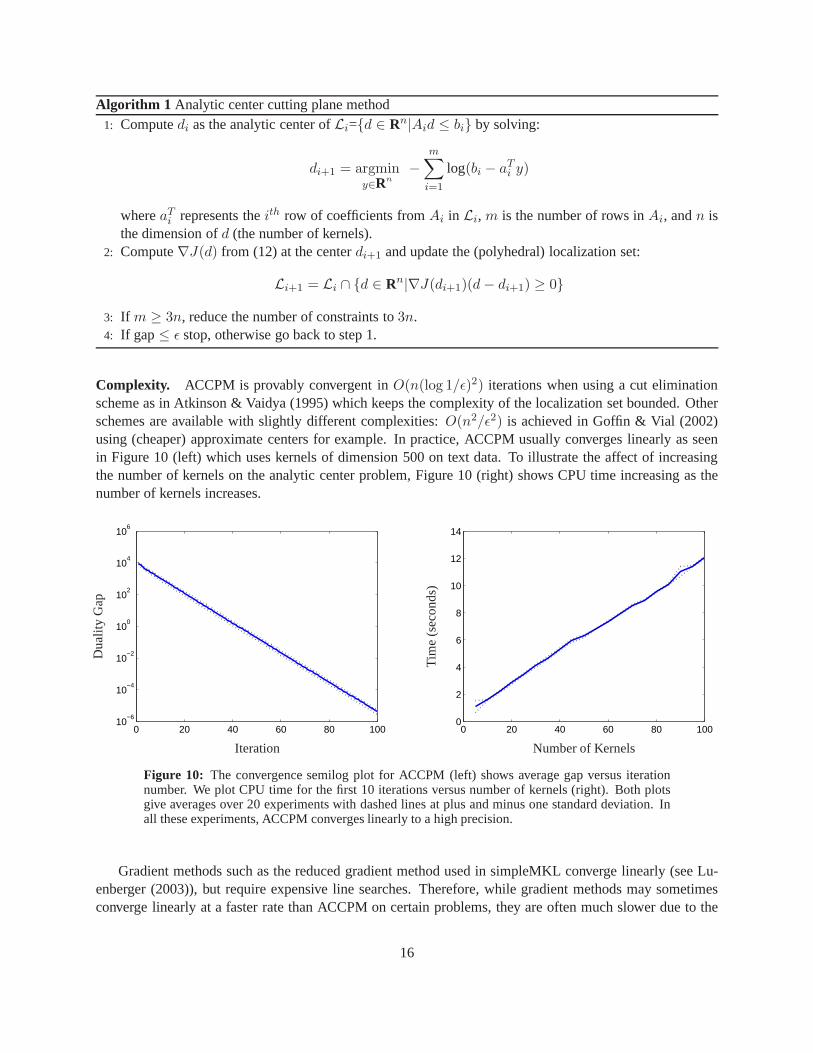
Algorithm 1 Analytic center cutting plane method1: Computedi as the analytic center ofLi={d ∈ Rn|Aid ≤ bi} by solving:

di+1 = argminy∈Rn

−m∑

i=1

log(bi − aTi y)

whereaTi represents theith row of coefficients fromAi in Li, m is the number of rows inAi, andn is

the dimension ofd (the number of kernels).2: Compute∇J(d) from (12) at the centerdi+1 and update the (polyhedral) localization set:

Li+1 = Li ∩ {d ∈ Rn|∇J(di+1)(d − di+1) ≥ 0}

3: If m ≥ 3n, reduce the number of constraints to3n.4: If gap≤ ǫ stop, otherwise go back to step 1.

Complexity. ACCPM is provably convergent inO(n(log 1/ǫ)2) iterations when using a cut eliminationscheme as in Atkinson & Vaidya (1995) which keeps the complexity of the localization set bounded. Otherschemes are available with slightly different complexities: O(n2/ǫ2) is achieved in Goffin & Vial (2002)using (cheaper) approximate centers for example. In practice, ACCPM usually converges linearly as seenin Figure 10 (left) which uses kernels of dimension 500 on text data. To illustrate the affect of increasingthe number of kernels on the analytic center problem, Figure10 (right) shows CPU time increasing as thenumber of kernels increases.

0 20 40 60 80 10010

−6

10−4

10−2

100

102

104

106

Du

ality

Gap

Iteration

0 20 40 60 80 1000

2

4

6

8

10

12

14

Tim

e(s

eco

nd

s)

Number of Kernels

Figure 10: The convergence semilog plot for ACCPM (left) shows averagegap versus iterationnumber. We plot CPU time for the first 10 iterations versus number of kernels (right). Both plotsgive averages over 20 experiments with dashed lines at plus and minus one standard deviation. Inall these experiments, ACCPM converges linearly to a high precision.

Gradient methods such as the reduced gradient method used insimpleMKL converge linearly (see Lu-enberger (2003)), but require expensive line searches. Therefore, while gradient methods may sometimesconverge linearly at a faster rate than ACCPM on certain problems, they are often much slower due to the

16

need to solve many SVM problems per iteration. Empirically,gradient methods tend to require many moregradient evaluations than the localization techniques discussed here. ACCPM computes the objective andgradient exactly once per iteration and the analytic centerproblem remains relatively cheap with respectto the SVM computation because the dimension of the analyticcentering problem (i.e. the number of ker-nels) is small in our application. Thresholding small kernel weights in MKL to zero can further reduce thedimension of the analytic center problem.

3.3 Computational Savings

As described above, ACCPM computes one SVM computation per iteration and converges linearly. Wecompare this method, which we denote accpmMKL, with the simpleMKL algorithm which uses a reducedgradient method and also converges fast but computes many more SVMs to perform line searches. TheSVMs in the line search are speeded up using warm-starting asdescribed in Rakotomamonjy et al. (2008)but in practice, we observe that savings in MKL from warm-starting often do not suffice to make this gradientmethod more efficient than ACCPM.

Few kernels are usually required in MKL because most kernelscan be eliminated more efficiently be-forehand using cross-validation, hence we use several families of kernels (linear, gaussian, and polynomial)but very few kernels from each family. Each experiment uses one linear kernel and the same number ofgaussian and polynomial kernels giving a total of 3, 7, and 11kernels (each normalized to unit trace) ineach experiment. We set the duality gap to .01 (a very loose gap) andC to 1000 (after cross-validationfor C ranging between 500 and 5000) for each experiment in order tocompare the algorithms on identicalproblems. For fairness, we compare simpleMKL with our implementation of accpmMKL using the sameSVM package in simpleMKL which allows warm-starting (The SVM package in simpleMKL is based onthe SVM-KM toolbox (Canu et al. 2005) and implemented in Matlab.). In the final column, we also givethe running time for accpmMKL using the LIBSVM solver without warm-starting. The following tablesdemonstrate computational efficiency and do not show predictive performance; both algorithms solve thesame optimization problem with the same stopping criterion. High precision for MKL does not significantlyincrease prediction performance. Results are averages over 20 experiments done on Linux 64-bit serverswith 2.6 GHz CPUs.

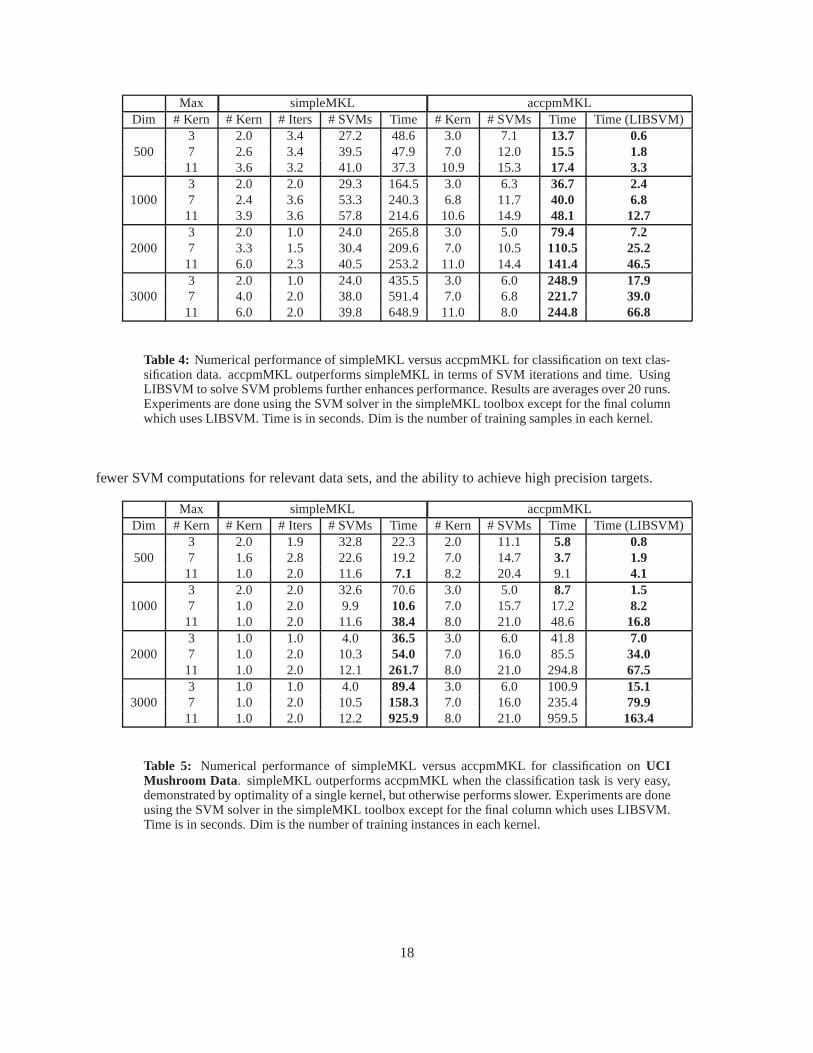
Table 4 shows that ACCPM is more efficient for the multiple kernel learning problem in a text classi-fication example. Savings from warm-starting SVM in simpleMKL do not overcome the benefit of fewerSVM computations at each iteration in accpmMKL. Furthermore, using a faster SVM solver such as LIB-SVM produces better performance even without warm-starting. The number of kernels used in accpmMKLis higher than with simpleMKL because of the very loose duality gap here. The reduced gradient methodof simpleMKL often stops at a much higher precision because the gap is checked after a line search thatcan achieve high precision in a single iteration and it is this higher precision that reduces the number ofkernels. However, for a slightly higher precision, simpleMKL will often stall or converge very slowly; themethod is very sensitive to the target precision. The accpmMKL method stops at the desired duality (mean-ing more kernels) because the gap is checked at each iteration during the linear convergence; however, theconvergence is much more stable and consistent for all data sets. For accpmMKL, the number of SVMs isequivalent to the number of iterations.

Table 5 shows an example where accpmMKL is outperformed by simpleMKL. This occurs when theclassification task is extremely easy and the optimal mix of kernels is a singleton. In this case, simpleMKLconverges with fewer SVMs. Note though that accpmMKL with LIBSVM is still faster here. Both examplesillustrate that simpleMKL trains many more SVMs whenever the optimal mix of kernels includes more thanone input kernel. Overall, accpmMKL has the advantages of consistent convergence rates for all data sets,

17

Max simpleMKL accpmMKLDim # Kern # Kern # Iters # SVMs Time # Kern # SVMs Time Time (LIBSVM)

5003 2.0 3.4 27.2 48.6 3.0 7.1 13.7 0.67 2.6 3.4 39.5 47.9 7.0 12.0 15.5 1.811 3.6 3.2 41.0 37.3 10.9 15.3 17.4 3.3

10003 2.0 2.0 29.3 164.5 3.0 6.3 36.7 2.47 2.4 3.6 53.3 240.3 6.8 11.7 40.0 6.811 3.9 3.6 57.8 214.6 10.6 14.9 48.1 12.7

20003 2.0 1.0 24.0 265.8 3.0 5.0 79.4 7.27 3.3 1.5 30.4 209.6 7.0 10.5 110.5 25.211 6.0 2.3 40.5 253.2 11.0 14.4 141.4 46.5

30003 2.0 1.0 24.0 435.5 3.0 6.0 248.9 17.97 4.0 2.0 38.0 591.4 7.0 6.8 221.7 39.011 6.0 2.0 39.8 648.9 11.0 8.0 244.8 66.8

Table 4: Numerical performance of simpleMKL versus accpmMKL for classification on text clas-sification data. accpmMKL outperforms simpleMKL in terms ofSVM iterations and time. UsingLIBSVM to solve SVM problems further enhances performance.Results are averages over 20 runs.Experiments are done using the SVM solver in the simpleMKL toolbox except for the final columnwhich uses LIBSVM. Time is in seconds. Dim is the number of training samples in each kernel.

fewer SVM computations for relevant data sets, and the ability to achieve high precision targets.

Max simpleMKL accpmMKLDim # Kern # Kern # Iters # SVMs Time # Kern # SVMs Time Time (LIBSVM)

5003 2.0 1.9 32.8 22.3 2.0 11.1 5.8 0.87 1.6 2.8 22.6 19.2 7.0 14.7 3.7 1.911 1.0 2.0 11.6 7.1 8.2 20.4 9.1 4.1

10003 2.0 2.0 32.6 70.6 3.0 5.0 8.7 1.57 1.0 2.0 9.9 10.6 7.0 15.7 17.2 8.211 1.0 2.0 11.6 38.4 8.0 21.0 48.6 16.8

20003 1.0 1.0 4.0 36.5 3.0 6.0 41.8 7.07 1.0 2.0 10.3 54.0 7.0 16.0 85.5 34.011 1.0 2.0 12.1 261.7 8.0 21.0 294.8 67.5

30003 1.0 1.0 4.0 89.4 3.0 6.0 100.9 15.17 1.0 2.0 10.5 158.3 7.0 16.0 235.4 79.911 1.0 2.0 12.2 925.9 8.0 21.0 959.5 163.4

Table 5: Numerical performance of simpleMKL versus accpmMKL for classification onUCIMushroom Data. simpleMKL outperforms accpmMKL when the classification task is very easy,demonstrated by optimality of a single kernel, but otherwise performs slower. Experiments are doneusing the SVM solver in the simpleMKL toolbox except for the final column which uses LIBSVM.Time is in seconds. Dim is the number of training instances ineach kernel.

18

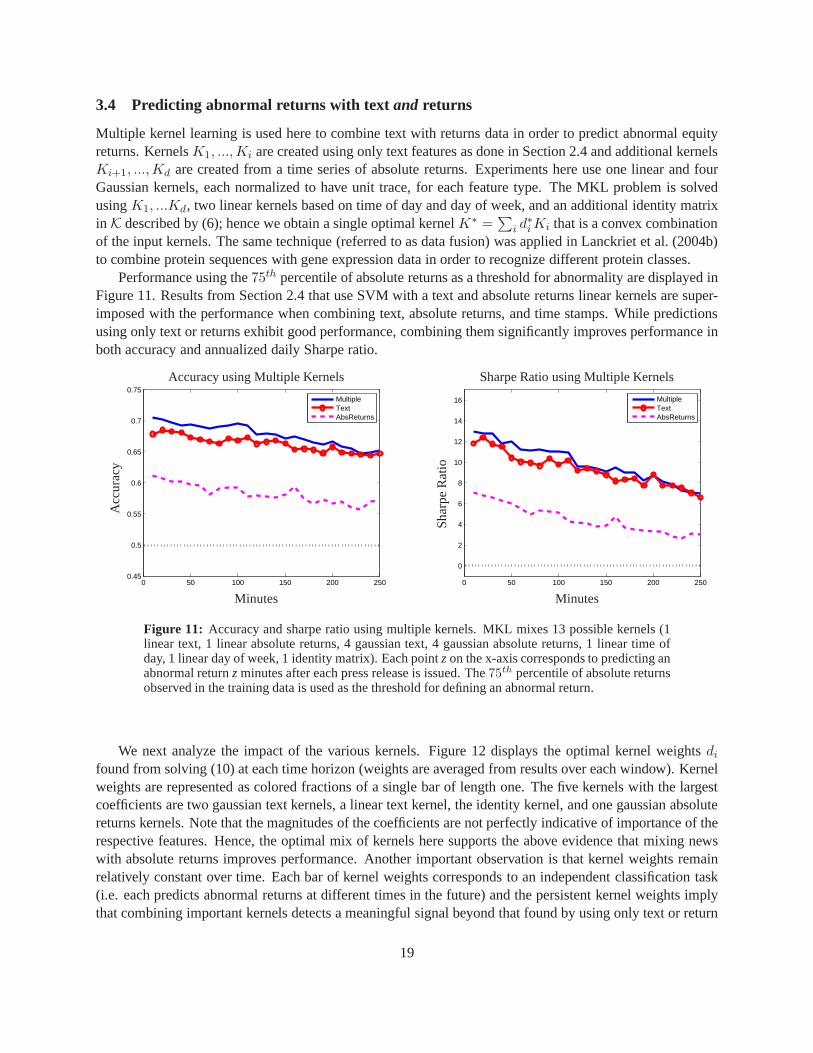
3.4 Predicting abnormal returns with text and returns

Multiple kernel learning is used here to combine text with returns data in order to predict abnormal equityreturns. KernelsK1, ...,Ki are created using only text features as done in Section 2.4 and additional kernelsKi+1, ...,Kd are created from a time series of absolute returns. Experiments here use one linear and fourGaussian kernels, each normalized to have unit trace, for each feature type. The MKL problem is solvedusingK1, ...Kd, two linear kernels based on time of day and day of week, and anadditional identity matrixin K described by (6); hence we obtain a single optimal kernelK∗ =

∑i d

∗i Ki that is a convex combination

of the input kernels. The same technique (referred to as datafusion) was applied in Lanckriet et al. (2004b)to combine protein sequences with gene expression data in order to recognize different protein classes.

Performance using the75th percentile of absolute returns as a threshold for abnormality are displayed inFigure 11. Results from Section 2.4 that use SVM with a text and absolute returns linear kernels are super-imposed with the performance when combining text, absolutereturns, and time stamps. While predictionsusing only text or returns exhibit good performance, combining them significantly improves performance inboth accuracy and annualized daily Sharpe ratio.

0 50 100 150 200 2500.45

0.5

0.55

0.6

0.65

0.7

0.75

MultipleTextAbsReturns

Accuracy using Multiple Kernels

Acc

ura

cy

Minutes0 50 100 150 200 250

0

2

4

6

8

10

12

14

16

MultipleTextAbsReturns

Sharpe Ratio using Multiple Kernels

Sh

arp

eR

atio

Minutes

Figure 11: Accuracy and sharpe ratio using multiple kernels. MKL mixes13 possible kernels (1linear text, 1 linear absolute returns, 4 gaussian text, 4 gaussian absolute returns, 1 linear time ofday, 1 linear day of week, 1 identity matrix). Each pointzon the x-axis corresponds to predicting anabnormal returnzminutes after each press release is issued. The75th percentile of absolute returnsobserved in the training data is used as the threshold for defining an abnormal return.

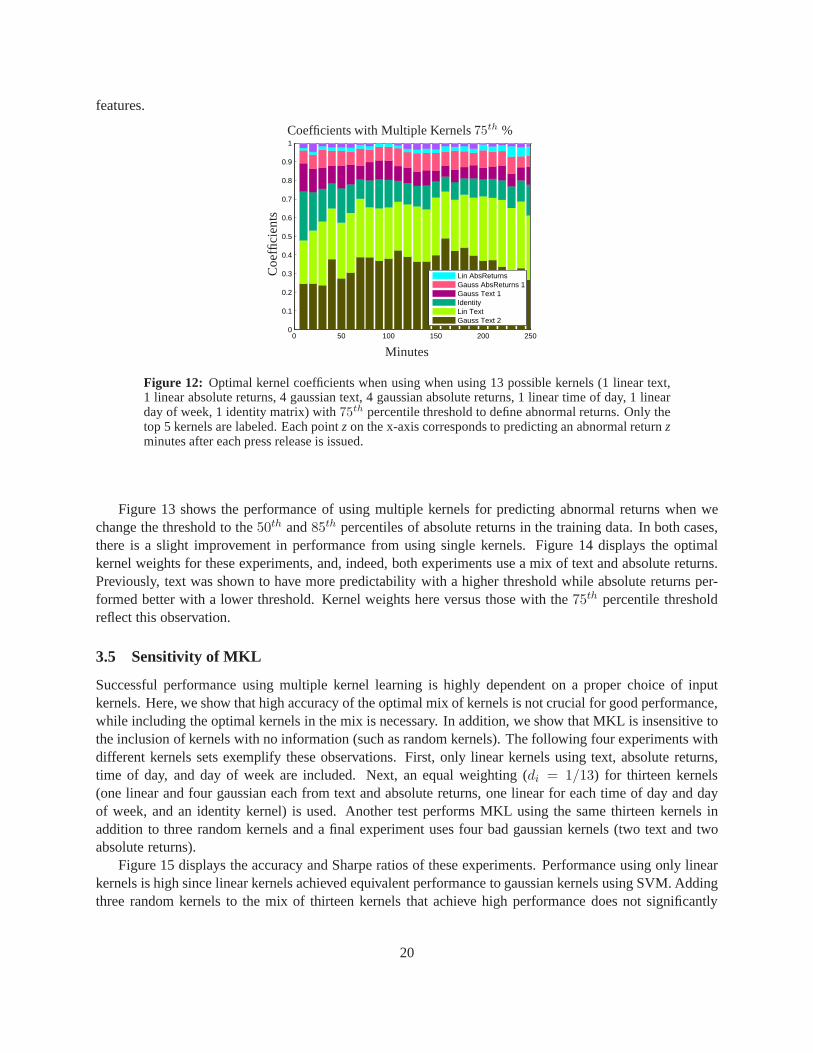
We next analyze the impact of the various kernels. Figure 12 displays the optimal kernel weightsdi

found from solving (10) at each time horizon (weights are averaged from results over each window). Kernelweights are represented as colored fractions of a single barof length one. The five kernels with the largestcoefficients are two gaussian text kernels, a linear text kernel, the identity kernel, and one gaussian absolutereturns kernels. Note that the magnitudes of the coefficients are not perfectly indicative of importance of therespective features. Hence, the optimal mix of kernels heresupports the above evidence that mixing newswith absolute returns improves performance. Another important observation is that kernel weights remainrelatively constant over time. Each bar of kernel weights corresponds to an independent classification task(i.e. each predicts abnormal returns at different times in the future) and the persistent kernel weights implythat combining important kernels detects a meaningful signal beyond that found by using only text or return

19

features.

0 50 100 150 200 2500

0.1

0.2

0.3

0.4

0.5

0.6

0.7

0.8

0.9

1

Lin AbsReturnsGauss AbsReturns 1Gauss Text 1IdentityLin TextGauss Text 2

Coefficients with Multiple Kernels75th %

Co

effic

ien

ts

Minutes

Figure 12: Optimal kernel coefficients when using when using 13 possible kernels (1 linear text,1 linear absolute returns, 4 gaussian text, 4 gaussian absolute returns, 1 linear time of day, 1 linearday of week, 1 identity matrix) with75th percentile threshold to define abnormal returns. Only thetop 5 kernels are labeled. Each pointz on the x-axis corresponds to predicting an abnormal returnzminutes after each press release is issued.

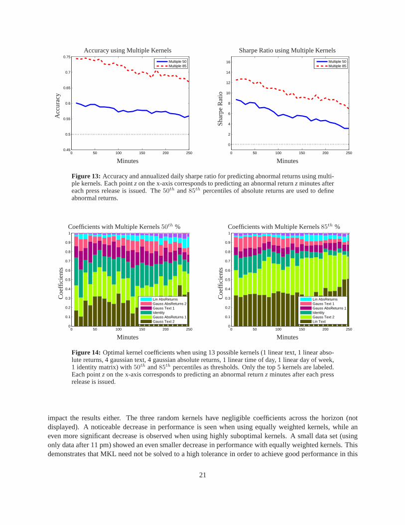
Figure 13 shows the performance of using multiple kernels for predicting abnormal returns when wechange the threshold to the50th and85th percentiles of absolute returns in the training data. In both cases,there is a slight improvement in performance from using single kernels. Figure 14 displays the optimalkernel weights for these experiments, and, indeed, both experiments use a mix of text and absolute returns.Previously, text was shown to have more predictability witha higher threshold while absolute returns per-formed better with a lower threshold. Kernel weights here versus those with the75th percentile thresholdreflect this observation.

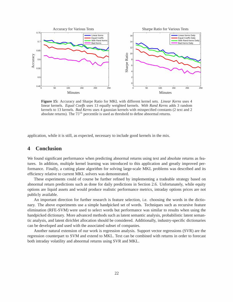
3.5 Sensitivity of MKL

Successful performance using multiple kernel learning is highly dependent on a proper choice of inputkernels. Here, we show that high accuracy of the optimal mix of kernels is not crucial for good performance,while including the optimal kernels in the mix is necessary.In addition, we show that MKL is insensitive tothe inclusion of kernels with no information (such as randomkernels). The following four experiments withdifferent kernels sets exemplify these observations. First, only linear kernels using text, absolute returns,time of day, and day of week are included. Next, an equal weighting (di = 1/13) for thirteen kernels(one linear and four gaussian each from text and absolute returns, one linear for each time of day and dayof week, and an identity kernel) is used. Another test performs MKL using the same thirteen kernels inaddition to three random kernels and a final experiment uses four bad gaussian kernels (two text and twoabsolute returns).

Figure 15 displays the accuracy and Sharpe ratios of these experiments. Performance using only linearkernels is high since linear kernels achieved equivalent performance to gaussian kernels using SVM. Addingthree random kernels to the mix of thirteen kernels that achieve high performance does not significantly

20

0 50 100 150 200 2500.45

0.5

0.55

0.6

0.65

0.7

0.75

Multiple 50Multiple 85

Accuracy using Multiple KernelsA

ccu

racy

Minutes0 50 100 150 200 250

0

2

4

6

8

10

12

14

16

Multiple 50Multiple 85

Sharpe Ratio using Multiple Kernels

Sh

arp

eR

atio

Minutes

Figure 13: Accuracy and annualized daily sharpe ratio for predicting abnormal returns using multi-ple kernels. Each pointzon the x-axis corresponds to predicting an abnormal returnzminutes aftereach press release is issued. The50th and85th percentiles of absolute returns are used to defineabnormal returns.

0 50 100 150 200 2500

0.1

0.2

0.3

0.4

0.5

0.6

0.7

0.8

0.9

1

Lin AbsReturnsGauss AbsReturns 2Gauss Text 1IdentityGauss AbsReturns 1Gauss Text 2

Coefficients with Multiple Kernels50th %

Co

effic

ien

ts

Minutes0 50 100 150 200 250

0

0.1

0.2

0.3

0.4

0.5

0.6

0.7

0.8

0.9

1

Lin AbsReturnsGauss Text 1Gauss AbsReturns 1IdentityGauss Text 2Lin Text

Coefficients with Multiple Kernels85th %C

oef

ficie

nts

Minutes

Figure 14: Optimal kernel coefficients when using 13 possible kernels (1 linear text, 1 linear abso-lute returns, 4 gaussian text, 4 gaussian absolute returns,1 linear time of day, 1 linear day of week,1 identity matrix) with50th and85th percentiles as thresholds. Only the top 5 kernels are labeled.Each pointz on the x-axis corresponds to predicting an abnormal returnz minutes after each pressrelease is issued.

impact the results either. The three random kernels have negligible coefficients across the horizon (notdisplayed). A noticeable decrease in performance is seen when using equally weighted kernels, while aneven more significant decrease is observed when using highlysuboptimal kernels. A small data set (usingonly data after 11 pm) showed an even smaller decrease in performance with equally weighted kernels. Thisdemonstrates that MKL need not be solved to a high tolerance in order to achieve good performance in this

21

0 50 100 150 200 2500.45

0.5

0.55

0.6

0.65

0.7

0.75

Linear KernsEqual CoeffsWith Rand KernsBad Kerns

Accuracy for Various TestsA

ccu

racy

Minutes0 50 100 150 200 250

0

2

4

6

8

10

12

14

16

Linear Kerns DailyEqual Coeffs DailyWith Rand Kerns DailyBad Kerns Daily

Sharpe Ratio for Various Tests

Sh

arp

eR

atio

Minutes

Figure 15: Accuracy and Sharpe Ratio for MKL with different kernel sets. Linear Kernsuses 4linear kernels.Equal Coeffsuses 13 equally weighted kernels.With Rand Kernsadds 3 randomkernels to 13 kernels.Bad Kernsuses 4 gaussian kernels with misspecified constants (2 text and 2absolute returns). The75th percentile is used as threshold to define abnormal returns.

application, while it is still, as expected, necessary to include good kernels in the mix.

4 Conclusion

We found significant performance when predicting abnormal returns using text and absolute returns as fea-tures. In addition, multiple kernel learning was introduced to this application and greatly improved per-formance. Finally, a cutting plane algorithm for solving large-scale MKL problems was described and itsefficiency relative to current MKL solvers was demonstrated.

These experiments could of course be further refined by implementing a tradeable strategy based onabnormal return predictions such as done for daily predictions in Section 2.6. Unfortunately, while equityoptions are liquid assets and would produce realistic performance metrics, intraday options prices are notpublicly available.

An important direction for further research is feature selection, i.e. choosing the words in the dictio-nary. The above experiments use a simple handpicked set of words. Techniques such as recursive featureelimination (RFE-SVM) were used to select words but performance was similar to results when using thehandpicked dictionary. More advanced methods such as latent semantic analysis, probabilistic latent seman-tic analysis, and latent dirichlet allocation should be considered. Additionally, industry-specific dictionariescan be developed and used with the associated subset of companies.

Another natural extension of our work is regression analysis. Support vector regressions (SVR) are theregression counterpart to SVM and extend to MKL. Text can be combined with returns in order to forecastboth intraday volatility and abnormal returns using SVR andMKL.

22

Acknowledgements

The authors are grateful to Jonathan Lange and Kevin Fan for superb research assistance. We would also liketo acknowledge support from NSF grant DMS-0625352, NSF CDI grant SES-0835550, a NSF CAREERaward, a Peek junior faculty fellowship and a Howard B. WentzJr. junior faculty award.

References

Andersen, T. G. & Bollerslev, T. (1997), ‘Intraday periodicity and volatility persistence in financial markets’,Journalof Empirical Finance4, 115–158.

Atkinson, D. S. & Vaidya, P. M. (1995), ‘A cutting plane algorithm for convex programming that uses analytic centers’,Mathematical Programming69, 1–43.

Austin, M. P., Bates, G., Dempster, M. A. H., Leemans, V. & Williams, S. N. (2004), ‘Adaptive systems for foreignexchange trading’,Quantitative Finance4, C37–C45.

Bach, F. R., Lanckriet, G. R. G. & Jordan, M. I. (2004), ‘Multiple kernel learning, conic duality, and the smo algo-rithm’, Proceedings of the 21st International Conference on Machine Learning.

Bertsekas, D. (1999),Nonlinear Programming, 2nd Edition, Athena Scientific.

Blei, D. M., Ng, A. Y. & Jordan, M. I. (2003), ‘Latent dirichlet allocation’,Journal of Machine Learning Research3, 993–1022.

Bollerslev, T., Chou, R. Y. & Kroner, K. F. (1992), ‘Arch modeling in finance: A review of the theory and empiricalevidence.’,Journal of Econometrics52, 5–59.

Bousquet, O. & Herrmann, D. J. L. (2003), ‘On the complexity of learning the kernel matrix’,Advances in NeuralInformation Processing Systems.

Canu, S., Grandvalet, Y., Guigue, V. & Rakotomamonjy, A. (2005), ‘Svm and kernel methods matlab toolbox’, Per-ception Systmes et Information, INSA de Rouen, Rouen, France.

Chang, C.-C. & Lin, C.-J. (2001), ‘LIBSVM: a library for support vector machines’. Software available athttp://www.csie.ntu.edu.tw/ cjlin/libsvm.

Cristianini, N. & Shawe-Taylor, J. (2000),An Introduction to Support Vector Machines and other kernel-based learn-ing methods, Cambridge University Press.

Deerwester, S., Dumais, S. T., Furnas, G. W., Landauer, T. K.& Harshman, R. (1990), ‘Indexing by latent semanticanalysis’,Journal of the American Society for Information Science41(6), 391–407.

Dempster, M. A. H. & Jones, C. M. (2001), ‘A real-time adapative trading system using genetic programming’,Quantitative Finance1, 397–413.

Ding, Z., Granger, C. W. J. & Engle, R. F. (1993), ‘A long memory property of stock market returns and a new model’,Journal of Empirical Finance1, 83–106.

Dumais, S., Platt, J., HHeckerman, D. & Sahami, M. (1998), ‘Inductive learning algoirhtms and representations fortext categorizations’,Proceedings of ACM0CIKM98.

Ederington, L. H. & Lee, J. H. (1993), ‘How markets process information: News releases and volatility’,The Journalof FinanceXLVIII(4), 1161–1191.

Fama, E. F. (1965), ‘The behavior of stock-market prices’,The Journal of Business38, 34–105.

Fung, G. P. C., Yu, J. X. & Lam, W. (2003), ‘Stock preiction: Integrating text mining approach using real-time news’,Proceedings of IEEE Conference on Computational Intelligence for Financial Engineeringpp. 395–402.

23

Gavrishchaka, V. V. & Banerjee, S. (2006), ‘Support vector machine as an efficient framework for stock marketvolatility forecasting’,Computational Management Science3, 147–160.

Goffin, J.-L. & Vial, J.-P. (2002), ‘Convex nondifferentiable optimization: A survey focused on the analytic centercutting plane method’,Optimization Methods and Software17(5), 805–867.

Hofmann, T. (2001), ‘Unsupervised learning by probabilistic latent semantic analysis’,Machine Learning42, 177–196.

Joachims, T. (2002),Learning to Classify Text Using Support Vector Machines: Methods, Theory and Algorithms,Kluwer Academic Publishers.

Kalev, P. S., Liu, W.-M., Pham, P. K. & Jarnecic, E. (2004), ‘Public information arrival and volatility of intraday stockreturns’,Journal of Banking and Finance28, 1441–1467.

Lanckriet, G. R. G., Bie, T. D., Cristianini, N., Jordan, M. I. & Noble, W. S. (2004b), ‘A statistical framework forgenomic data fusion’,Bioinformatics20, 2626–2635.

Lanckriet, G. R. G., Cristianini, N., Bartlett, P., Ghaoui,L. E. & Jordan, M. I. (2004a), ‘Learning the kernel matrixwith semidefinite programming’,Journal of Machine Learning Research5, 27–72.

Lavrenko, V., Schmill, M., Lawrie, D., Ogilvie, P., Jensen,D. & Allan, J. (2000), ‘Mining of concurrent text and timeseries’,Proceedings of 6th ACM SIGKDD Int. Conference on Knowledge Discovery and Data Mining.

Luenberger, D. (2003),Linear and Nonlinear Programming, 2nd Edition, Kluwer Academic Publishers.

M.-A.Mittermayer & Knolmayer, G. (2006a), ‘Newscats: A news categorization and trading system’,Proceedings ofthe Sixth International Conference on Data Mining.

M.-A.Mittermayer & Knolmayer, G. (2006b), ‘Text mining systems for predicting the market response to news: Asurvey’,Working Paper No. 184, Institute of Information Systems, Univ. of Bern, Bern.

Malliaris, M. & Salchenberger, L. (1996), ‘Using neural networks to forecast the s & p 100 implied volatility’,Neuro-computing10, 183–195.

Micchelli, C. A. & Pontil, M. (2007), ‘Feature space perspectives for learning the kernel’,Machine Learning66, 297–319.

Mitchell, M. L. & Mulherin, J. H. (1994), ‘The impact of public information on the stock market’,The Journal ofFinanceXLIX(3), 923–950.

Ong, C. S., Smola, A. J. & Williamson, R. C. (2005), ‘Learningthe kernel with hyperkernels’,Journal of MachineLearning Research6, 1043–1071.

Rakotomamonjy, A., Bach, F., Canu, S. & Grandvalet, Y. (2008), ‘Simplemkl’, Journal of Machine Learning Research. to appear.

Robertson, C. S., Geva, S. & Wolff, R. C. (2007), ‘News aware volatility forecasting: Is the content of news impor-tant?’,Proc. of the 6th Australasian Data Mining Conference (AusDM’07), Gold Coast, Australia.

Sonnenberg, S., Ratsch, G., Schafer, C. & Scholkopf, B. (2006), ‘Large scale multiple kernel learning’,Journal ofMachine Learning Research7, 1531–1565.

Taylor, S. (1986),Modelling financial time series, New York, John Wiley & Sons.

Taylor, S. J. & Xu, X. (1997), ‘The incremental volatility information in one million foreign exchange quotations’,Journal of Empirical Finance4, 317–340.

Thomas, J. D. (2003),News and Trading Rules, Dissertation, Carnegie Mellon University, Pittsburgh, PA.

Wood, R. A., McInish, T. H. & Ord, J. K. (1985), ‘An investigation of transactions data for nyse stocks’,The Journalof FinanceXL(3), 723–739.

24

Wuthrich, B., Cho, V., Leung, S., Perammunetilleke, D., Sankaran, K., Zhang, J. & Lam, W. (1998), ‘Daily predictionof major stock indices from textual web data’,Proceedings of 4th ACM SIGKDD Int. Conference on KnowledgeDiscovery and Data Mining.

Zien, A. & Ong, C. S. (2007), ‘Multiclass multiple kernel learning’, Proceedings of the 24th International Conferenceon Machine Learning.

25