Embed Size (px)
Citation preview
Date:
13290 Evening Creek Drive S, Suite 250San Diego, CA 92128T 858.480.2000F 858.792.8932www.ata-e.com
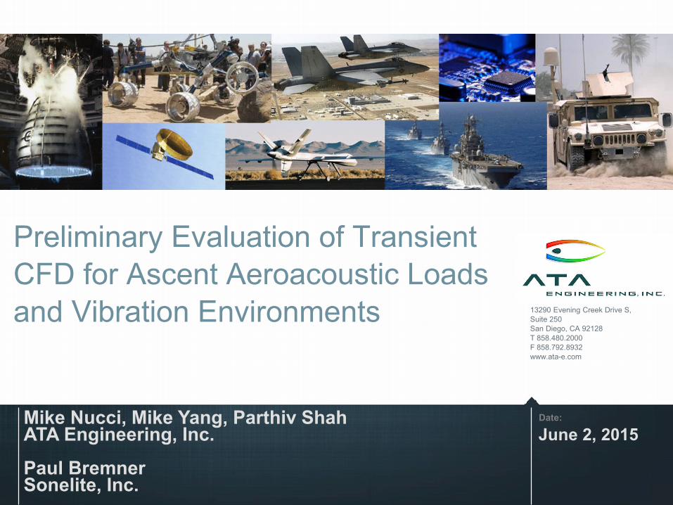
Preliminary Evaluation of Transient CFD for Ascent Aeroacoustic Loads and Vibration Environments
Mike Nucci, Mike Yang, Parthiv ShahATA Engineering, Inc.
Paul BremnerSonelite, Inc.
June 2, 2015

Spacecraft and Launch Vehicles Workshop 2015
Presentation Outline
MotivationUnsteady CFD analysis of expansion ramp at transonic speedsDerivation of Corcos CoefficientsWavenumber analysis of CFD resultsSummaryFuture Work
2

Spacecraft and Launch Vehicles Workshop 2015
Motivation
1. Locally high, inhomogenous aero loads can drive problematic random vibration environments
2. Limited # Kulites in wind tunnel, under-resolves loading• Compensate with high uncertainty margins or “maxi-max” approach• Could lead to over-conservative vibration qualification levels
3. CFD offers high spatial resolution, everywhere• Define spatial distribution of PSD loading ?• Define spatial correlation of loading ?• Sufficient time length can be limitation => Supplement with testing
4. Do locally high aeroloads really increase random vibration response ?
• What is correct – and practical - use of CFD aeroloads to predict random vibration ?
3
Spacecraft and Launch Vehicles Workshop 2015
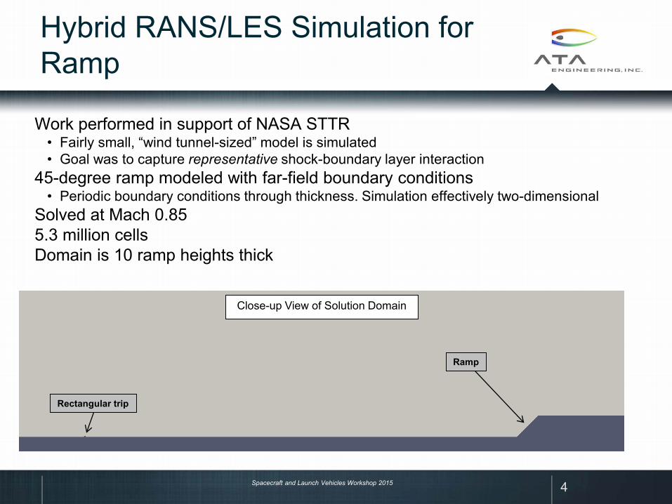
Hybrid RANS/LES Simulation for Ramp
Work performed in support of NASA STTR• Fairly small, “wind tunnel-sized” model is simulated• Goal was to capture representative shock-boundary layer interaction
45-degree ramp modeled with far-field boundary conditions • Periodic boundary conditions through thickness. Simulation effectively two-dimensional
Solved at Mach 0.855.3 million cellsDomain is 10 ramp heights thick
4
Rectangular trip
Ramp
Close-up View of Solution Domain
Spacecraft and Launch Vehicles Workshop 2015
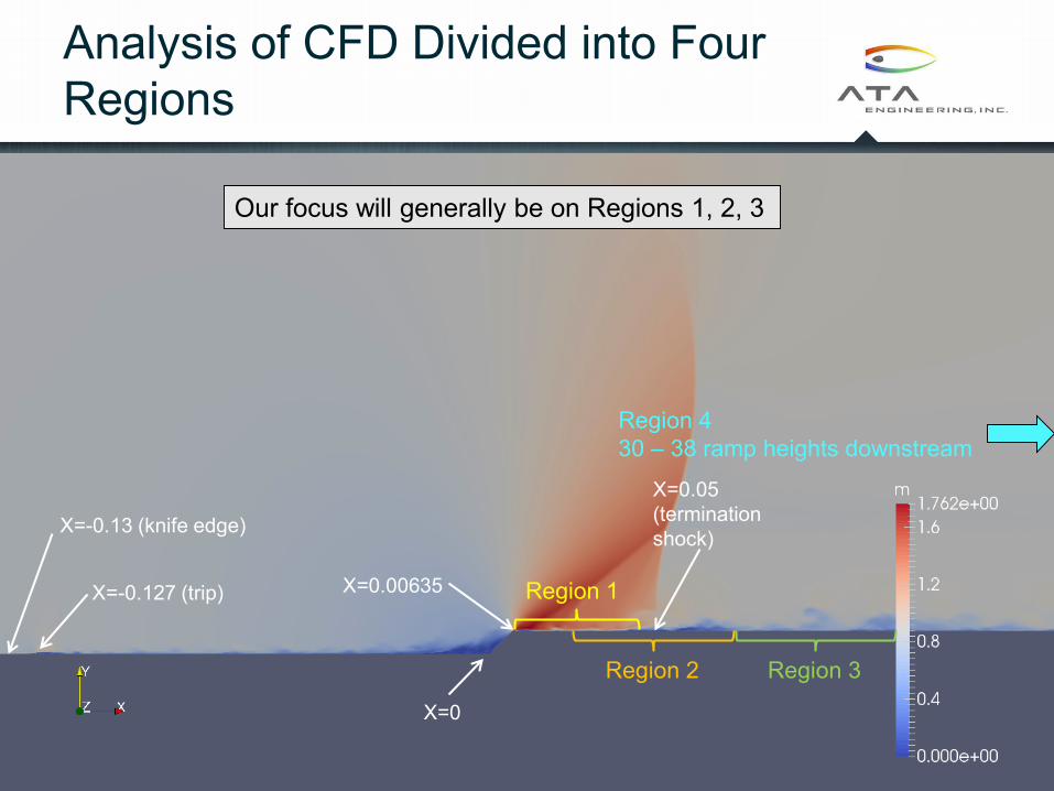
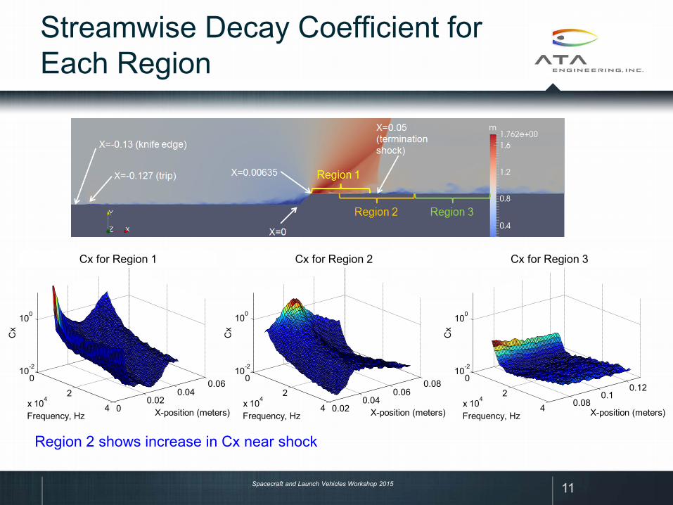
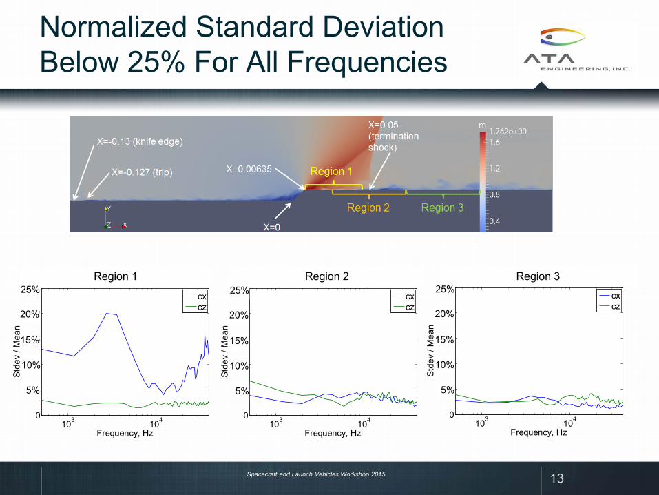
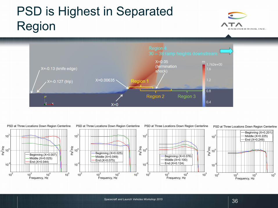
Analysis of CFD Divided into Four Regions
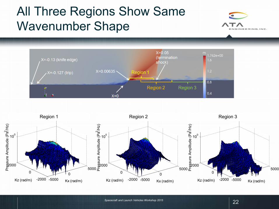
X=0
X=0.00635
X=0.05 (termination shock)
X=-0.127 (trip)
X=-0.13 (knife edge)
Region 1
Region 2
Region 430 – 38 ramp heights downstream
Region 3
Our focus will generally be on Regions 1, 2, 3
Spacecraft and Launch Vehicles Workshop 2015
-0.1 -0.05 0 0.05 0.1 0.15 0.2 0.25 0.3-0.1
-0.05
0
0.05
0.1
0.15
X-Position (m)
Del
ta C
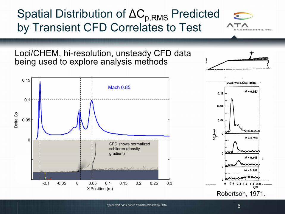
pSpatial Distribution of ΔCp,RMS Predicted by Transient CFD Correlates to Test
6
CFD shows normalized schlieren (density gradient)
Loci/CHEM, hi-resolution, unsteady CFD data being used to explore analysis methods
Robertson, 1971.
Mach 0.85
Spacecraft and Launch Vehicles Workshop 2015
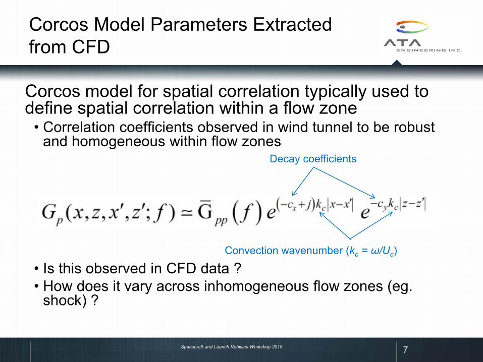
Corcos model for spatial correlation typically used to define spatial correlation within a flow zone• Correlation coefficients observed in wind tunnel to be robust
and homogeneous within flow zones
• Is this observed in CFD data ?• How does it vary across inhomogeneous flow zones (eg.
shock) ?
Corcos Model Parameters Extracted from CFD
7
Decay coefficients
Convection wavenumber (kc = ω/Uc)
Spacecraft and Launch Vehicles Workshop 2015 8
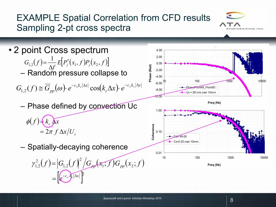
EXAMPLE Spatial Correlation from CFD resultsSampling 2-pt cross spectra
• 2 point Cross spectrum
– Random pressure collapse to
– Phase defined by convection Uc
– Spatially-decaying coherence
( ) ( ) ykcc
xkcpp
cycx exkeGfG ∆−∆− ⋅∆⋅≅ cos)(2,1 ω
-10.00
-8.00
-6.00
-4.00
-2.00
0.00
2.00
4.00
10 100 1000 10000
Freq (Hz)
Pha
se (R
ad)
PhasePoint49_Point50
Uc = 28 m/s over 10mm
0.01
0.10
1.00
10 100 1000 10000
Freq (Hz)
Coh
eren
ce
Coh 49-50
Cx=0.25 over 10mm
( ) ( ) ( )[ ]fxPfxPEf
fG jj ,,121
*2,1 ∆
=
( )c
c
Uxfxkf∆=
∆=π
φ2
( ) ( ) ( ) ( )
[ ]221
22,1
22,1 ;;
xkc
pppp
cxe
fxGfxGfGf∆−=
=γ

Spacecraft and Launch Vehicles Workshop 2015
PSD is Highest in Separated Region
9
102 103 104 105
10-2
100
102
Frequency, Hz
Pa2 /H
z
PSD at Three Locations Down Region Centerline
Beginning (X=0.007)Middle (X=0.025)End (X=0.044)
102 103 104 105
10-2
100
102
Frequency, Hz
Pa2 /H
z
PSD at Three Locations Down Region Centerline
Beginning (X=0.025)Middle (X=0.049)End (X=0.075)
102 103 104 105
10-2
100
102
Frequency, Hz
Pa2 /H
z
PSD at Three Locations Down Region Centerline
Beginning (X=0.076)Middle (X=0.100)End (X=0.124)
PSD in Region 1 PSD in Region 2 PSD in Region 3
PSD in Region 4 ~ 1 Pa^2/Hz over entire region
Spacecraft and Launch Vehicles Workshop 2015
CORCOS COEFFICIENTS DERIVED FROM CFD
10
Spacecraft and Launch Vehicles Workshop 2015
0
24x 104 0.08
0.10.12
10-2
100
X-position (meters)
Cx along streamline in center of panel
Frequency, Hz
Cx
02
4x 10⁴
0.020.04
0.060.08
10-2
100
X-position (meters)
Cx along streamline in center of panel
Frequency, Hz
Cx
0
24x 104
00.02
0.040.06
10-2
100
X-position (meters)
Cx along streamline in center of panel
Frequency, Hz
Cx
Streamwise Decay Coefficient for Each Region
11
Cx for Region 1 Cx for Region 2 Cx for Region 3
Region 2 shows increase in Cx near shock

Spacecraft and Launch Vehicles Workshop 2015
0 0.01 0.02 0.03 0.04 0.050
0.5
1
1.5
2
2.5
X-Position (meters)
Cx
Cx along streamline in center of panel
3000 Hz10000 Hz25000 Hz40000 Hz
0.06 0.08 0.1 0.12 0.14 0.160
0.5
1
1.5
2
2.5
X-Position (meters)
Cx
Cx along streamline in center of panel
3000 Hz10000 Hz25000 Hz40000 Hz
Streamwise Decay Coefficient Down Center of Panel
12
Cx for Region 1 Cx for Region 2 Cx for Region 3
Increase at low frequencies expected due to boundary layer thickness limitation on large eddy correlation length [Ref: Bull, C&R “modified” CORCOS model]
Spacecraft and Launch Vehicles Workshop 2015
103 1040
0.05
0.1
0.15
0.2
0.25
Frequency, HzSt
dev
/ Mea
n
Normalized Standard Deviation across panel
cxcz
103 1040
0.05
0.1
0.15
0.2
0.25
Frequency, Hz
Stde
v / M
ean
Normalized Standard Deviation across panel
cxcz
103 1040
0.05
0.1
0.15
0.2
0.25
Frequency, Hz
Stde
v / M
ean
Normalized Standard Deviation across panel
cxcz
Normalized Standard Deviation Below 25% For All Frequencies
13
Region 1 Region 2 Region 325%
20%
15%
10%
5%
25%
20%
15%
10%
5%
25%
20%
15%
10%
5%
Spacecraft and Launch Vehicles Workshop 2015
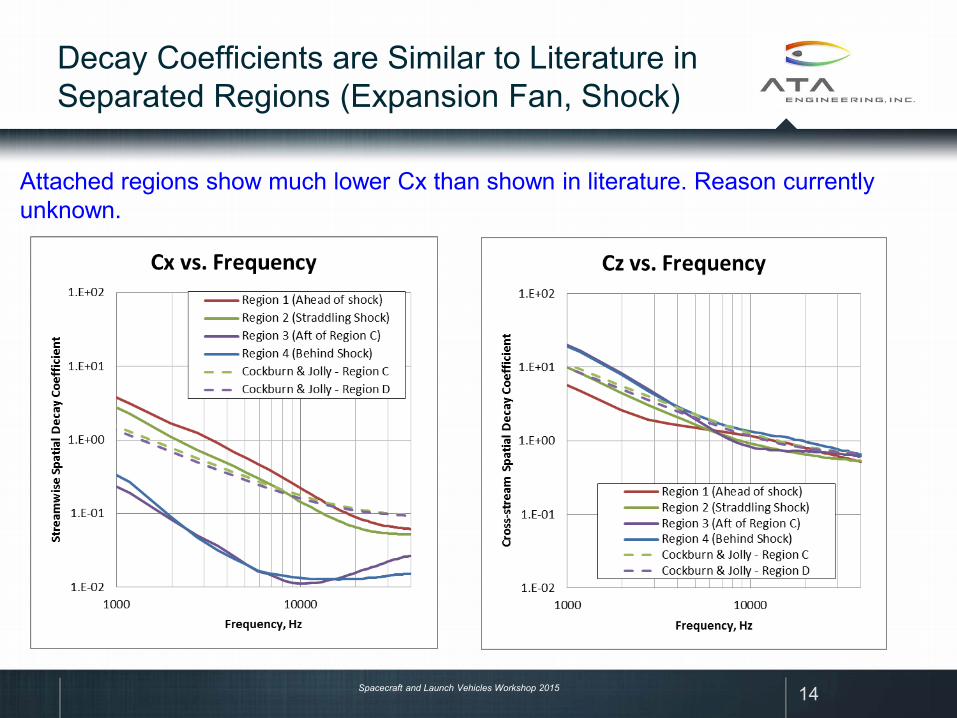
Decay Coefficients are Similar to Literature in Separated Regions (Expansion Fan, Shock)
14
Attached regions show much lower Cx than shown in literature. Reason currently unknown.
Spacecraft and Launch Vehicles Workshop 2015
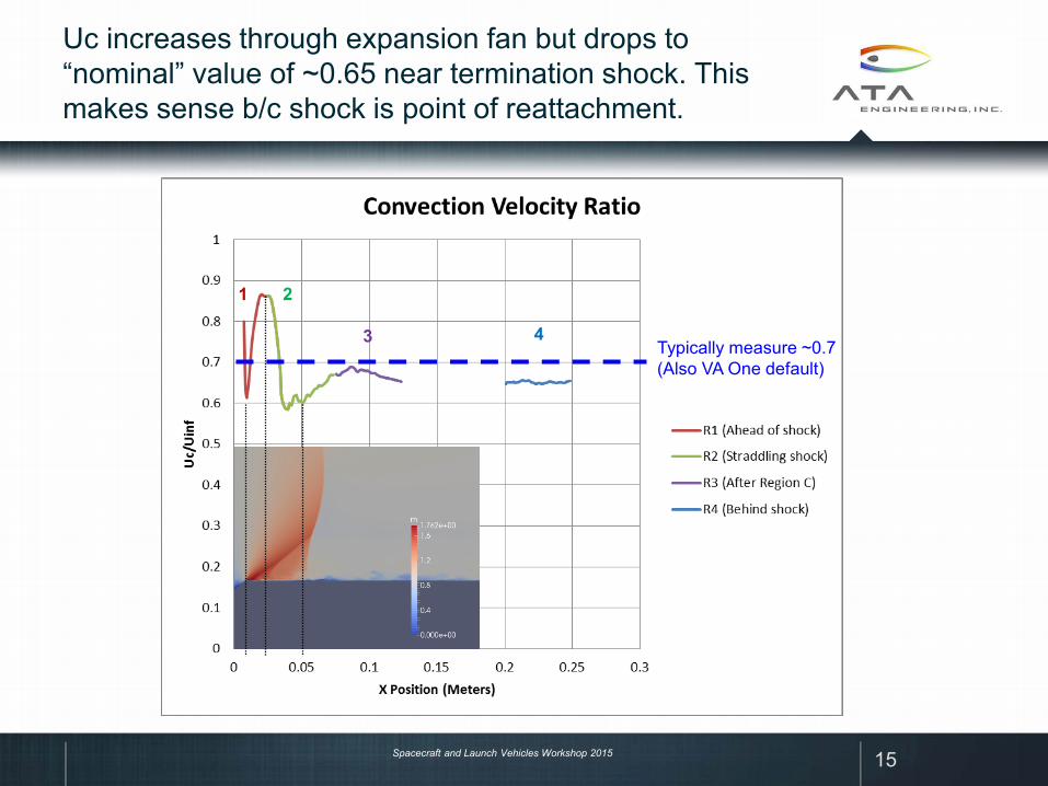
Uc increases through expansion fan but drops to “nominal” value of ~0.65 near termination shock. This makes sense b/c shock is point of reattachment.
15
Typically measure ~0.7(Also VA One default)
1 2
3 4
Spacecraft and Launch Vehicles Workshop 2015
SPATIAL WAVE-INTEGRATED (AVERAGED) SPATIAL CORRELATION FROM CFD
16
Spacecraft and Launch Vehicles Workshop 2015
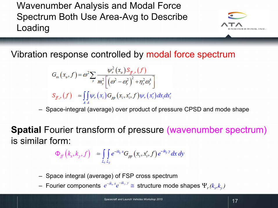
Wavenumber Analysis and Modal Force Spectrum Both Use Area-Avg to Describe Loading
Vibration response controlled by modal force spectrum
– Space-integral (average) over product of pressure CPSD and mode shape
Spatial Fourier transform of pressure (wavenumber spectrum) is similar form:
– Space integral (average) of FSP cross spectrum– Fourier components structure mode shapes Ψr (kx,ky )
17
Spacecraft and Launch Vehicles Workshop 2015
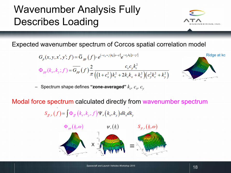
Wavenumber Analysis Fully Describes Loading
Expected wavenumber spectrum of Corcos spatial correlation model
– Spectrum shape defines “zone-averaged” kc, cx, cy
Modal force spectrum calculated directly from wavenumber spectrum
18
X =
( ),pp k ωΦ ( )r kψ ( ), ,ff rS k ω
Ridge at kc
Spacecraft and Launch Vehicles Workshop 2015
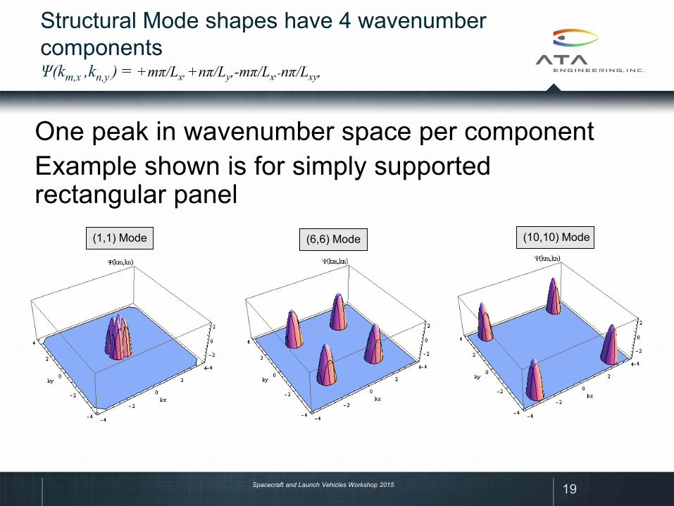
Structural Mode shapes have 4 wavenumber componentsΨ(km,x ,kn,y ) = +mπ/Lx, +nπ/Ly,-mπ/Lx,-nπ/Lxy,
One peak in wavenumber space per componentExample shown is for simply supported rectangular panel
19
(1,1) Mode (6,6) Mode (10,10) Mode
Spacecraft and Launch Vehicles Workshop 2015
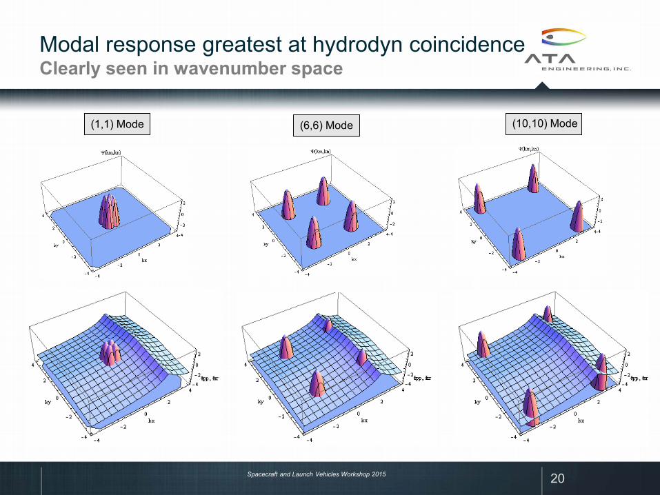
Modal response greatest at hydrodyn coincidenceClearly seen in wavenumber space
20
(1,1) Mode (6,6) Mode (10,10) Mode
Spacecraft and Launch Vehicles Workshop 2015
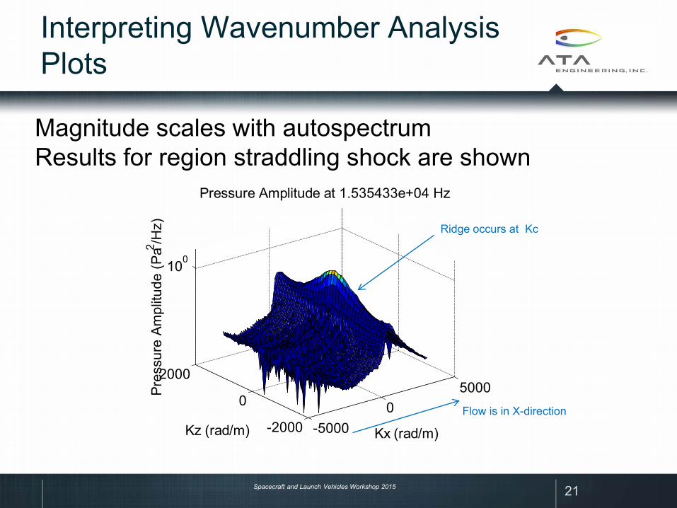
Interpreting Wavenumber Analysis Plots
21
Magnitude scales with autospectrumResults for region straddling shock are shown
-50000
5000
-2000
0
2000
100
Kx (rad/m)
Pressure Amplitude at 1.535433e+04 Hz
Kz (rad/m)
Pres
sure
Am
plitu
de (P
a2 /Hz) Ridge occurs at Kc
Flow is in X-direction
Spacecraft and Launch Vehicles Workshop 2015
-50000
5000
-2000
0
2000
100
Kx (rad/m)
Pressure Amplitude at 1.535433e+04 Hz
Kz (rad/m)
Pres
sure
Am
plitu
de (P
a2 /Hz)
-50000
5000
-2000
0
2000
100
Kx (rad/m)
Pressure Amplitude at 1.535433e+04 Hz
Kz (rad/m)
Pres
sure
Am
plitu
de (P
a2 /Hz)
-50000
5000
-2000
0
2000
100
Kx (rad/m)
Pressure Amplitude at 1.535433e+04 Hz
Kz (rad/m)
Pres
sure
Am
plitu
de (P
a2 /Hz)
All Three Regions Show Same Wavenumber Shape
22
Region 1 Region 2 Region 3
Spacecraft and Launch Vehicles Workshop 2015
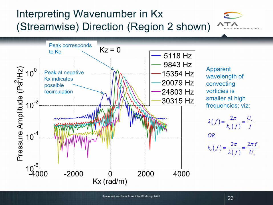
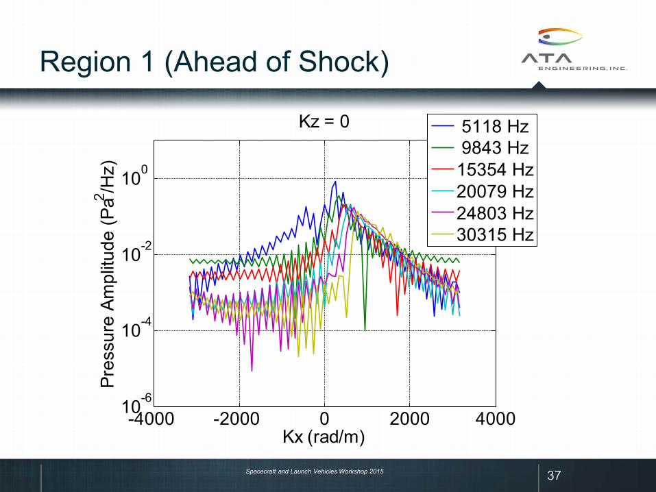
Interpreting Wavenumber in Kx(Streamwise) Direction (Region 2 shown)
23
-4000 -2000 0 2000 400010-6
10-4
10-2
100
Kx (rad/m)
Pres
sure
Am
plitu
de (P
a2 /Hz)
Kz = 0
5118 Hz 9843 Hz15354 Hz20079 Hz24803 Hz30315 Hz
Apparent wavelength of convectingvorticies is smaller at high frequencies; viz:
( ) ( )
( ) ( )
2
2 2
c
c
cc
Ufk f f
ORfk f
f U
πλ
π πλ
= =
= =
Peak corresponds to Kc
Peak at negative Kx indicates possible recirculation
Spacecraft and Launch Vehicles Workshop 2015
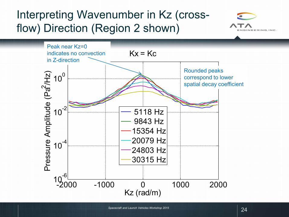
Interpreting Wavenumber in Kz (cross-flow) Direction (Region 2 shown)
24
-2000 -1000 0 1000 200010-6
10-4
10-2
100
Kz (rad/m)
Pres
sure
Am
plitu
de (P
a2 /Hz)
Kx = Kc
5118 Hz 9843 Hz15354 Hz20079 Hz24803 Hz30315 Hz
Peak near Kz=0 indicates no convection in Z-direction
Rounded peaks correspond to lower spatial decay coefficient
Spacecraft and Launch Vehicles Workshop 2015
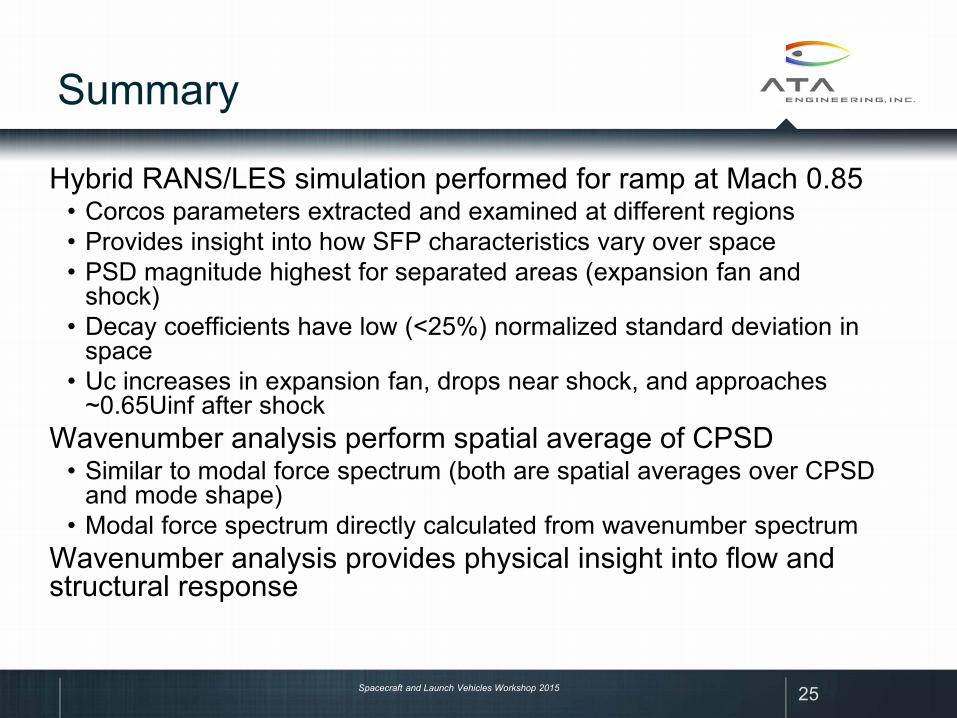
Summary
Hybrid RANS/LES simulation performed for ramp at Mach 0.85• Corcos parameters extracted and examined at different regions• Provides insight into how SFP characteristics vary over space• PSD magnitude highest for separated areas (expansion fan and
shock)• Decay coefficients have low (<25%) normalized standard deviation in
space• Uc increases in expansion fan, drops near shock, and approaches
~0.65Uinf after shockWavenumber analysis perform spatial average of CPSD• Similar to modal force spectrum (both are spatial averages over CPSD
and mode shape)• Modal force spectrum directly calculated from wavenumber spectrum
Wavenumber analysis provides physical insight into flow and structural response
25
Spacecraft and Launch Vehicles Workshop 2015
Future Work
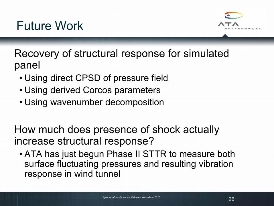
Recovery of structural response for simulated panel• Using direct CPSD of pressure field• Using derived Corcos parameters• Using wavenumber decomposition
How much does presence of shock actually increase structural response? • ATA has just begun Phase II STTR to measure both
surface fluctuating pressures and resulting vibration response in wind tunnel
26
Spacecraft and Launch Vehicles Workshop 2015
APPENDIX
27
Spacecraft and Launch Vehicles Workshop 2015
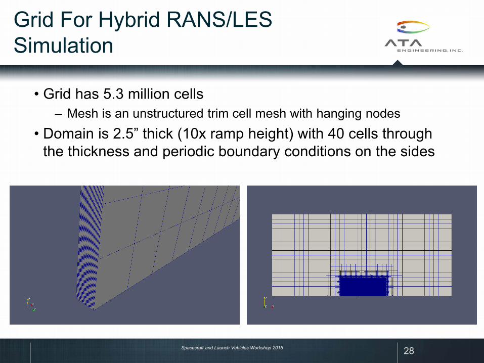
Grid For Hybrid RANS/LES Simulation
28
• Grid has 5.3 million cells– Mesh is an unstructured trim cell mesh with hanging nodes
• Domain is 2.5” thick (10x ramp height) with 40 cells through the thickness and periodic boundary conditions on the sides
Spacecraft and Launch Vehicles Workshop 2015
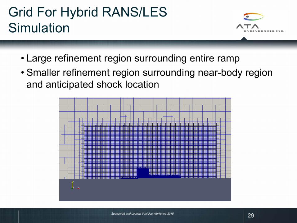
Grid For Hybrid RANS/LES Simulation
29
• Large refinement region surrounding entire ramp• Smaller refinement region surrounding near-body region
and anticipated shock location
Spacecraft and Launch Vehicles Workshop 2015
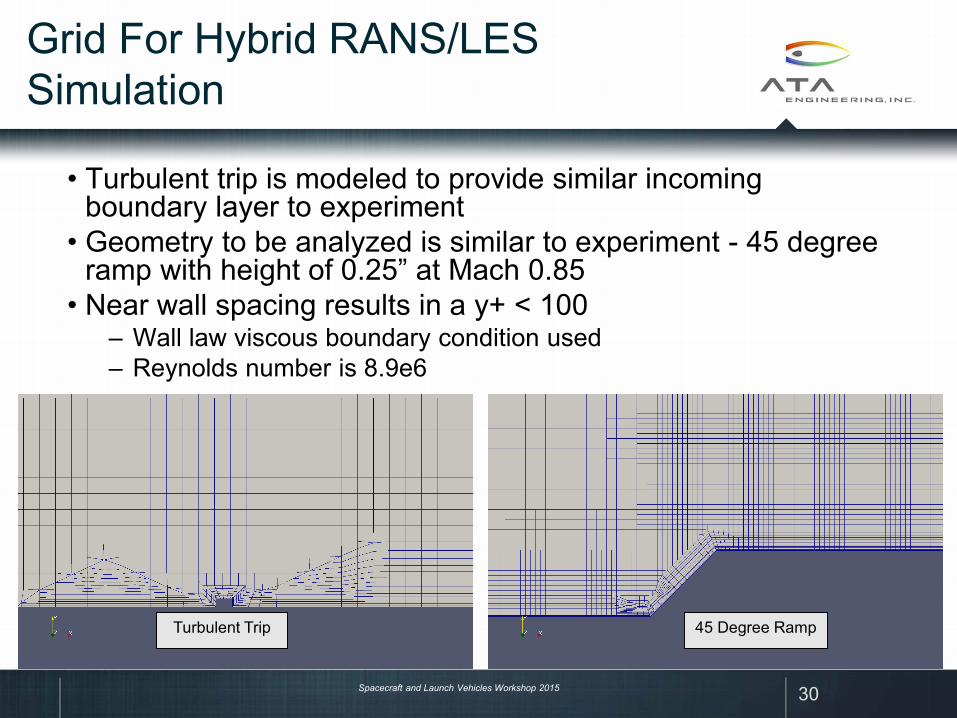
Grid For Hybrid RANS/LES Simulation
30
• Turbulent trip is modeled to provide similar incoming boundary layer to experiment
• Geometry to be analyzed is similar to experiment - 45 degree ramp with height of 0.25” at Mach 0.85
• Near wall spacing results in a y+ < 100– Wall law viscous boundary condition used– Reynolds number is 8.9e6
Turbulent Trip 45 Degree Ramp
Spacecraft and Launch Vehicles Workshop 2015
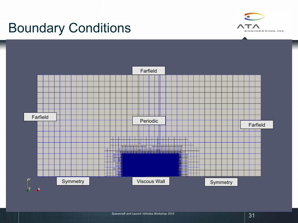
Boundary Conditions
31
Farfield
FarfieldFarfield
Viscous WallSymmetry Symmetry
Periodic
Spacecraft and Launch Vehicles Workshop 2015
Entire solution domain
32
Spacecraft and Launch Vehicles Workshop 2015
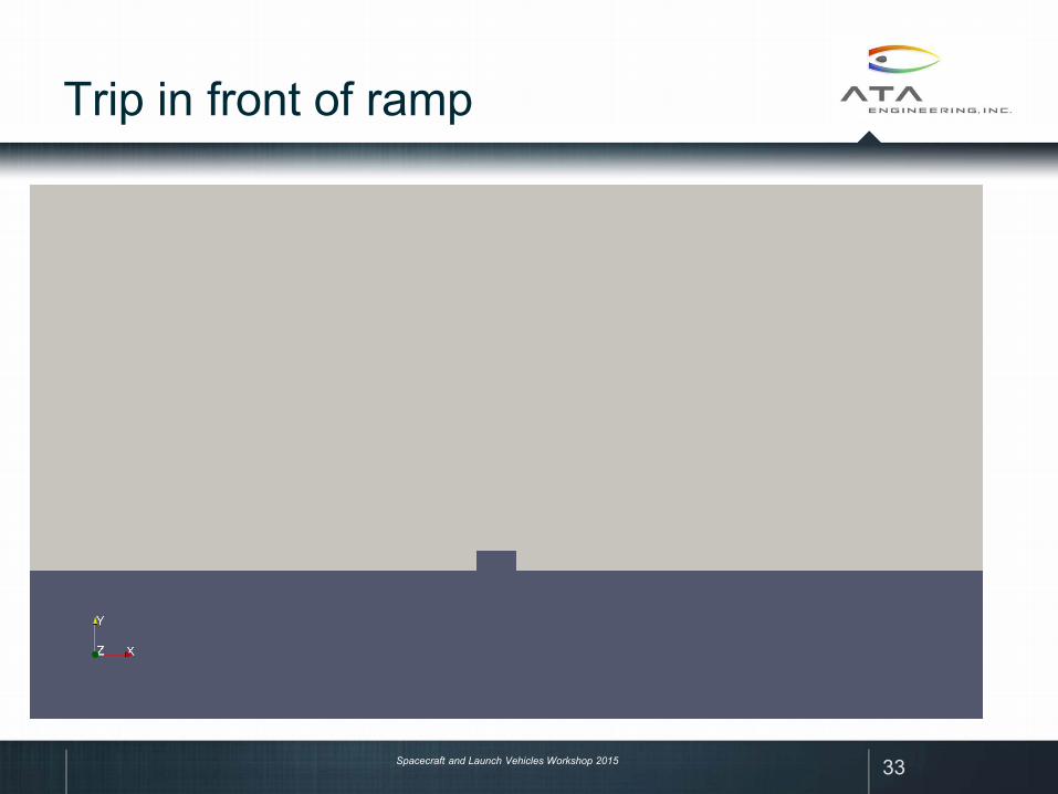
Trip in front of ramp
33
Spacecraft and Launch Vehicles Workshop 2015
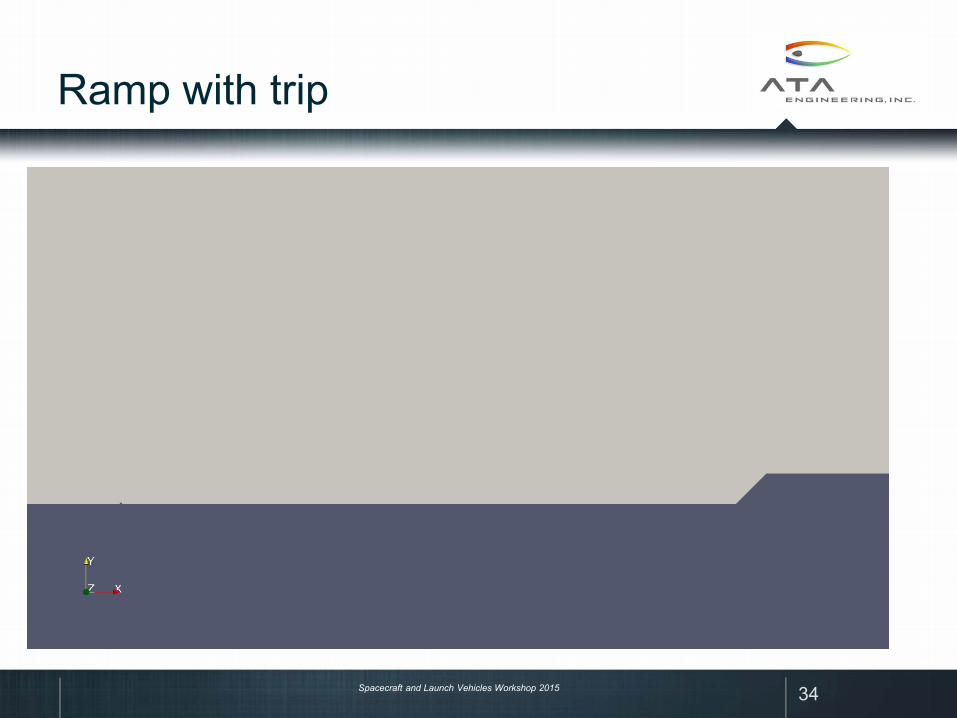
Ramp with trip
34
Spacecraft and Launch Vehicles Workshop 2015
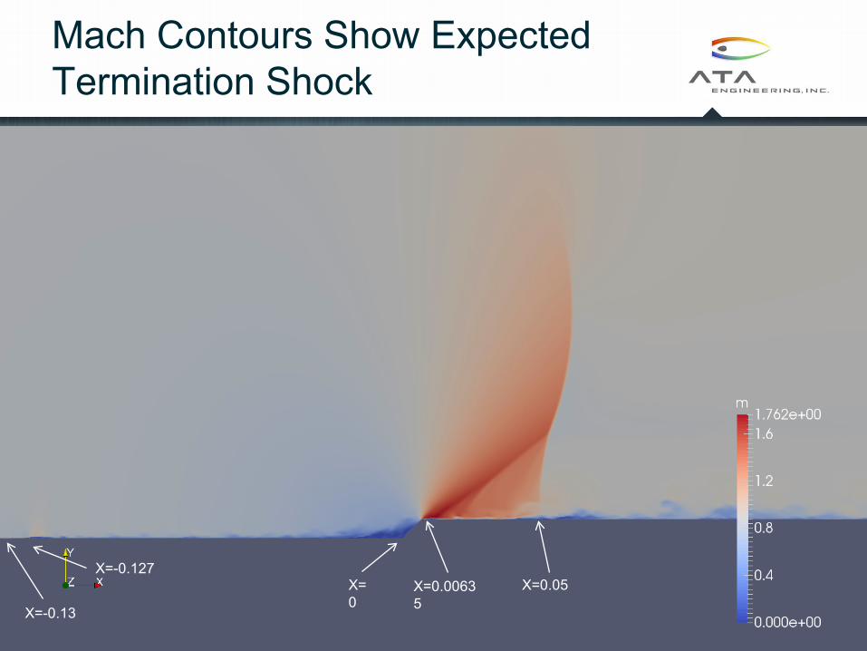
Mach Contours Show Expected Termination Shock
X=0
X=0.00635
X=0.05X=-0.127
X=-0.13
Spacecraft and Launch Vehicles Workshop 2015
PSD is Highest in Separated Region
36
102 103 104 105
10-2
100
102
Frequency, Hz
Pa2 /H
z
PSD at Three Locations Down Region Centerline
Beginning (X=0.007)Middle (X=0.025)End (X=0.044)
102 103 104 105
10-2
100
102
Frequency, Hz
Pa2 /H
z
PSD at Three Locations Down Region Centerline
Beginning (X=0.025)Middle (X=0.049)End (X=0.075)
102 103 104 105
10-2
100
102
Frequency, Hz
Pa2 /H
z
PSD at Three Locations Down Region Centerline
Beginning (X=0.076)Middle (X=0.100)End (X=0.124)
102 103 104 105
10-2
100
102
Frequency, Hz
Pa2 /H
z
PSD at Three Locations Down Region Centerline
Beginning (X=0.201)Middle (X=0.225)End (X=0.249)
Spacecraft and Launch Vehicles Workshop 2015
Region 1 (Ahead of Shock)
37
-4000 -2000 0 2000 400010-6
10-4
10-2
100
Kx (rad/m)
Pres
sure
Am
plitu
de (P
a2 /Hz)
Kz = 0
5118 Hz 9843 Hz15354 Hz20079 Hz24803 Hz30315 Hz

Spacecraft and Launch Vehicles Workshop 2015
Region 3 (Aft of region 2)
38
-4000 -2000 0 2000 400010-6
10-4
10-2
100
Kx (rad/m)
Pres
sure
Am
plitu
de (P
a2 /Hz)
Kz = 0
5118 Hz 9843 Hz15354 Hz20079 Hz24803 Hz30315 Hz
Apparent wavelength of convectingvorticies is smaller at high frequencies; viz:
( ) ( )
( ) ( )
2
2 2
c
c
cc
Ufk f f
ORfk f
f U
πλ
π πλ
= =
= =
Spacecraft and Launch Vehicles Workshop 2015
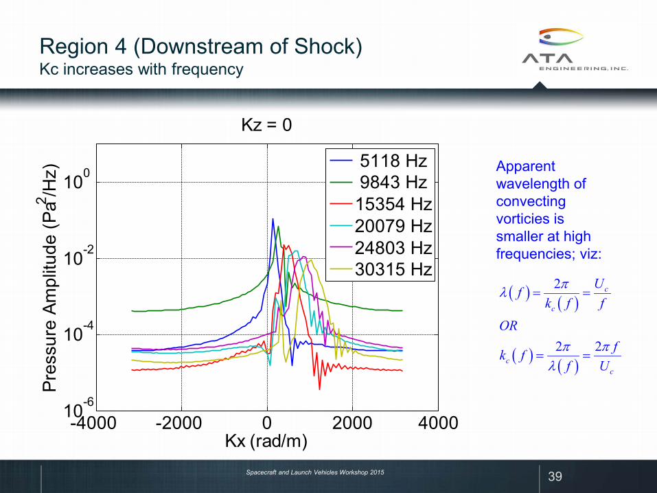
Region 4 (Downstream of Shock)Kc increases with frequency
39
-4000 -2000 0 2000 400010-6
10-4
10-2
100
Kx (rad/m)
Pres
sure
Am
plitu
de (P
a2 /Hz)
Kz = 0
5118 Hz 9843 Hz15354 Hz20079 Hz24803 Hz30315 Hz
Apparent wavelength of convectingvorticies is smaller at high frequencies; viz:
( ) ( )
( ) ( )
2
2 2
c
c
cc
Ufk f f
ORfk f
f U
πλ
π πλ
= =
= =
Spacecraft and Launch Vehicles Workshop 2015
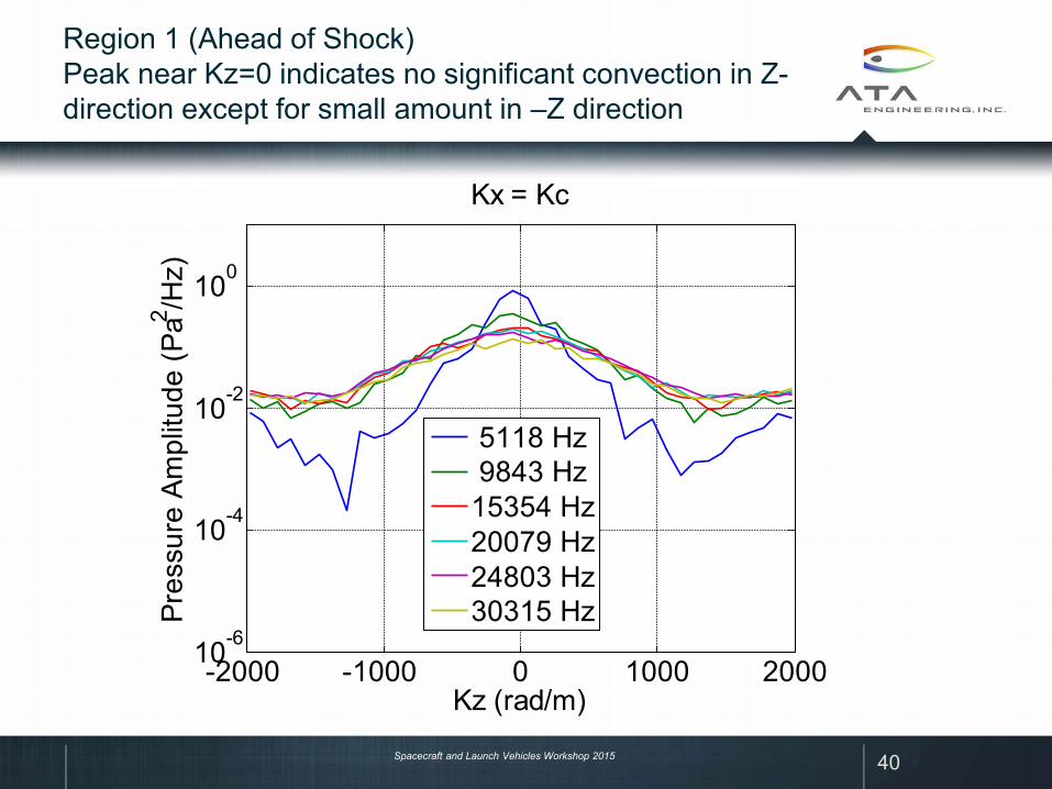
Region 1 (Ahead of Shock)Peak near Kz=0 indicates no significant convection in Z-direction except for small amount in –Z direction
40
-2000 -1000 0 1000 200010-6
10-4
10-2
100
Kz (rad/m)
Pres
sure
Am
plitu
de (P
a2 /Hz)
Kx = Kc
5118 Hz 9843 Hz15354 Hz20079 Hz24803 Hz30315 Hz
Spacecraft and Launch Vehicles Workshop 2015
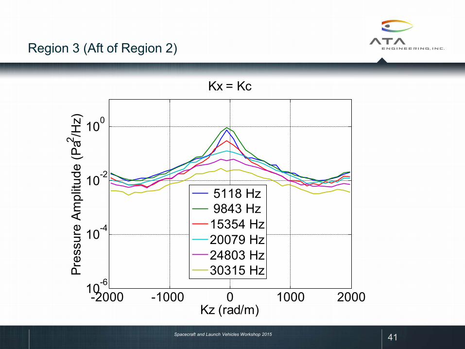
Region 3 (Aft of Region 2)
41
-2000 -1000 0 1000 200010-6
10-4
10-2
100
Kz (rad/m)
Pres
sure
Am
plitu
de (P
a2 /Hz)
Kx = Kc
5118 Hz 9843 Hz15354 Hz20079 Hz24803 Hz30315 Hz
Spacecraft and Launch Vehicles Workshop 2015
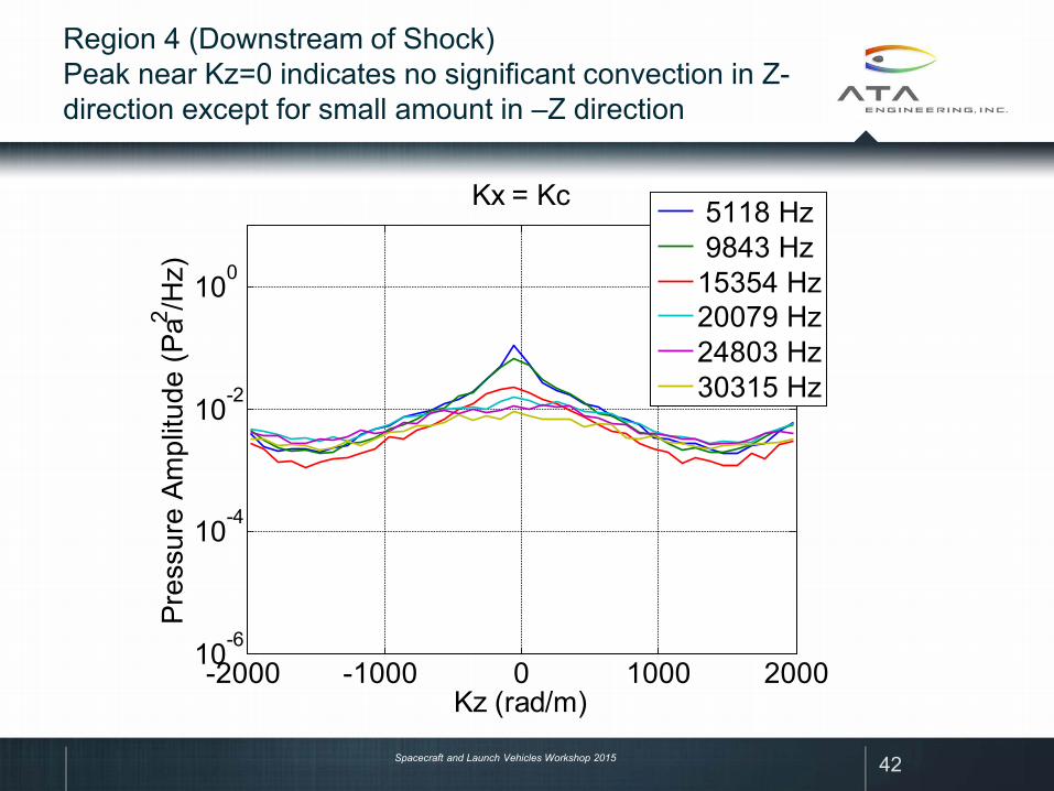
Region 4 (Downstream of Shock)Peak near Kz=0 indicates no significant convection in Z-direction except for small amount in –Z direction
42
-2000 -1000 0 1000 200010-6
10-4
10-2
100
Kz (rad/m)
Pres
sure
Am
plitu
de (P
a2 /Hz)
Kx = Kc
5118 Hz 9843 Hz15354 Hz20079 Hz24803 Hz30315 Hz