Embed Size (px)
Citation preview

Preliminary Technical and Economic Feasibility Study of
Binary Power Plant for Chiweta Geothermal Field, Malawi
Tufwane Mwagomba
Thesis of 60 ECTS credits
Master of Science in Sustainable Energy
Iceland School of Energy
January 2016

Preliminary Technical and Economic Feasibility Study of
Binary Power Plant for Chiweta Geothermal Field, Malawi
Tufwane Mwagomba
60 ECTS thesis submitted to the School of Science and Engineering
at Reykjavík University in partial fulfillment
of the requirements for the degree of
Master of Science in Sustainable Energy – Iceland School of Energy
January 2016
Student:
___________________________________________
Tufwane Mwagomba
Supervisor(s):
___________________________________________
Dr. Einar Jón Ásbjörnsson
___________________________________________
Examiner:
___________________________________________
Dr. María Sigríður Guðjónsdóttir

Preliminary Technical and Economic Feasibility Study of
Binary Power Plant for Chiweta Geothermal Field, Malawi
Tufwane Mwagomba
Thesis of 60 ECTS credits submitted to the School of Science and Engineering
at Reykjavík University in partial fulfillment
of the requirements for the degree of
Master of Science in Sustainable Energy
January 2016
Supervisor:
Dr. Einar Jón Ásbjörnsson
Assistant Professor, Reykjavík University, Iceland
Examiner:
Dr. María Sigríður Guðjónsdóttir
Reykjavik University.


i
Abstract Insufficient electricity generation capacity that is failing to meet the ever increasing electricity
demand coupled with low electrification rate and low per capita consumption of electricity in
Malawi are some of the reasons causing Malawi to search for alternative sources of energy to
complement the current predominantly hydro generation capacity. Having manifestation of
geothermal in some parts of the country, geothermal energy is being considered for development
in line with having a diverse national energy mix.
By virtue of its location in the western branch of the East African Rift System, which is relatively
cooler than the eastern branch due to its lower geothermal temperature gradient, developing
geothermal in Malawi for electricity generation can focus on utilizing binary technology until
such a time when subsurface studies proves otherwise. The field of focus that has high promising
geothermal potential in Malawi with the highest geothermal water surface temperature measured
so far, is Chiweta geothermal field measuring 79°C.
Technical and economic analysis of four binary power plant models has been done using
Engineering Equations Solver software as a technical analysis tool and NPV, IRR and Discounted
Payback Period as economic analysis tools. Technical and economic performance of all the four
models is satisfactory with wet cooled recuperative binary model emerging the best performer in
both analyses. However, due to issues of pressure drop in heat exchangers and the fact that the
model’s performance is similar to a wet cooled basic binary, it is recommended for Malawi to
develop a wet cooled basic binary for its promising Chiweta field which would generate a net
power of 10 MW at a total development capital cost of approximately US $49.5 million. The
capital cost can be recovered in 17 years at a discount rate of 12 % while selling electricity at the
prescribed tariff of US $0.105/kWh as informed by Malawi’s Feed-in Tariff policy.

ii

iii
Table of contents
Abstract .......................................................................................................................................... i
i. List of Tables ........................................................................................................................ iv
ii. List of Figures ...................................................................................................................... iv
Acknowledgements ..................................................................................................................... vii
1.0. Introduction ....................................................................................................................... 1
2.0. Background ....................................................................................................................... 2
2.1. Geothermal in Malawi ................................................................................................... 2
2.2. Description of Chiweta geothermal field ...................................................................... 6
2.3. Geothermal utilization ................................................................................................... 8
2.4. Electricity supply in Malawi ....................................................................................... 10
3.0. Geothermal power plant technologies ............................................................................. 13
3.1. Steam flash power plants ............................................................................................. 13
3.2. Binary cycle power plant ............................................................................................. 15
3.3. Combined cycle power plant ....................................................................................... 18
4.0. Technical analysis of the technology applicable for Chiweta system ............................. 20
4.1. Thermodynamic analysis ............................................................................................. 20
4.2. Power plant cooling system ......................................................................................... 25
4.3. Consideration of scaling potential ............................................................................... 30
4.4. Choice of working fluid in binary plant ...................................................................... 32
5.0. Modelling of the binary power plant ............................................................................... 35
5.1. Boundary conditions ................................................................................................... 35
5.2. Modelling of scenarios and results .............................................................................. 42
6.0. Economic analysis of the applicable technology ............................................................ 54
6.1. Cost of field development ........................................................................................... 54
6.2. Cost of power plant’s major equipment ...................................................................... 55
6.3. Civil, electrical and controls cost ................................................................................ 56
6.4. Total costs of developing the models .......................................................................... 57
6.5. Financial ratios analysis .............................................................................................. 59
7.0. Conclusion ....................................................................................................................... 64
8.0. Recommendations ........................................................................................................... 66
9.0. References ....................................................................................................................... 67
10.0. Appendices .................................................................................................................. 71

iv
i. List of Tables
Table 1: Categories of geothermal systems based on temperature, enthalpy and physical state
(Saemundsson, et al., 2011) .......................................................................................................... 9
Table 2: Energy Mix Projections 2000 – 2050. Source: adapted from DoE (2003) ................... 11
Table 3: Properties of binary plant working fluids. Source: modified from DiPippo, (2012) .... 33
Table 4: Common boundary conditions for the models .............................................................. 42
Table 5: Results of the Dry and Wet cooled basic binary plant .................................................. 47
Table 6: Results of Dry cooled and Wet cooled recuperative binary plant. ................................ 50
Table 7: Recuperator effect on wet and dry cooled models ........................................................ 52
Table 8: Geothermal field cost estimates .................................................................................... 54
Table 9: Estimated costs of power plant major equipment ......................................................... 56
Table 10: Summary of civil works and electrical and control equipment costs .......................... 57
Table 11: Total cost of developing the models ........................................................................... 57
Table 12: O&M cost for the four models .................................................................................... 59
Table 13: Estimated annual revenue for the models ................................................................... 60
Table 14: Internal Rate of Return for the models ........................................................................ 62
ii. List of Figures
Figure 1: Geological map of Malawi. Source: (Mdala, 2015) ...................................................... 3
Figure 2: The East African Rift System. Source (Chorowicz, 2005) ......................................... 4
Figure 3: Showing (A) seismic reflection profile for L. Malawi, (B) and (C) Inferred
lithospheric cross-section of Malawi and Kenya. Source: (Chorowicz, 2005) ............................. 5
Figure 4: Location of Chiweta hot spring. Source: adapted from (Dulanya, et al., 2010) ............ 7
Figure 5: Chiweta climate showing temperature and precipitation. Source: adapted from
(Climate Data, 2015) ..................................................................................................................... 7
Figure 6: A hot spring in Chiweta with sulphur deposits, discharging into Mphizi stream. (Photo
taken on 09/08/2015) ..................................................................................................................... 8
Figure 7: Lindal’s geothermal utilization diagram. Source: modified from (Ragnarsson, 2006)
..................................................................................................................................................... 10
Figure 8: Process flow diagram of a Single flash power plant .................................................... 13
Figure 9: Typical T-s diagram for a single flash power plant ..................................................... 14
Figure 10: Process flow diagram for a double flash power plant ................................................ 15
Figure 11: Typical T-s diagram for a double flash power plant .................................................. 15
Figure 12: Process flow diagram of a dry cooled Binary cycle power plant............................... 16
Figure 13: A typical T-s diagram for a binary cycle using dry fluid ........................................... 17
Figure 14: Schematic diagram of a Kalina cycle power plant. Source: Adapted from
Valdimarsson (2010) ................................................................................................................... 18
Figure 15: Combined single flash and binary power plant.......................................................... 19
Figure 16: Vaporizer and preheater section of the binary cycle .................................................. 21
Figure 17: Binary turbine ............................................................................................................ 23
Figure 18: Power plant condensing unit ...................................................................................... 24
Figure 19: Fluid circulation pump ............................................................................................... 25
Figure 20: Schematic diagram of a wet cooling system .............................................................. 27
Figure 21: schematic diagram of the dry cooling system ............................................................ 29

v
Figure 22: Silica solubility curve. Source: (Fournier & Rowe, 1977) ........................................ 32
Figure 23: A T-s diagram for (a) wet fluid, (b) isentropic fluid and (c) dry fluid. Source: Bao &
Zao (2013) ................................................................................................................................... 34
Figure 24: Calculated silica concentration in geothermal fluid................................................... 36
Figure 25: T-s diagram for various working fluids ..................................................................... 37
Figure 26: Vaporizer pressure and turbine work output of working fluids ................................. 38
Figure 27: Reinjection temperature and turbine work output of working fluids ......................... 39
Figure 28: Optimal vaporizer pressure for isopentane in dry cooled basic model ...................... 39
Figure 29: Reinjection temperature considering generator output and vaporizer pressure ......... 40
Figure 30: Optimal vaporizer pressure for dry cooled basic binary ............................................ 40
Figure 31: Required geothermal fluid mass flow for dry cooled basic binary model ................. 43
Figure 32: T-s diagram for the dry cooled basic binary cycle ..................................................... 44
Figure 33: T-h diagram for the dry cooled basic binary cycle .................................................... 44
Figure 34: P-h diagram for the dry cooled basic binary cycle .................................................... 45
Figure 35: Heat transfer process in the preheater and vaporizer for the basic binary model ...... 46
Figure 36: Heat transfer process in the condenser for the basic binary model ............................ 46
Figure 37: T-s diagram for the dry cooled recuperative binary cycle ......................................... 48
Figure 38: T-h diagram for the dry cooled recuperative binary cycle ......................................... 48
Figure 39: P-h diagram for the dry cooled recuperative binary cycle ......................................... 49
Figure 40: Summary of technical analysis of power for the binary models ................................ 51
Figure 41: Comparison of equipment size and fluids for the binary models .............................. 53
Figure 42: Total cost of models................................................................................................... 57
Figure 43: Cost of generating a kW for the models .................................................................... 58
Figure 44: Net Present Value for the models .............................................................................. 61
Figure 45: Discounted net cash flow for payback period ............................................................ 63

vi

vii
Acknowledgements I sincerely thank the UNU-GTP for offering me an opportunity to undertake my studies under this
course in Iceland. The UNU-GTP members of staff led by the program director Ludvik S.
Georgsson were so supportive to make both my stay and studies as comfortable as possible. Being
a first fellow under the arrangement with my University, it meant the UNU had to learn and do
some things for the first time. And it has all made what I have become today.
A special thanks my supervisor Einar Jón Ásbjörnsson for the guidance and support during the
thesis and making sure that I was focused. The scheduled weekly meetings always reminded me
to have a new thing for the next meeting and this helped to accelerate my work.
Inputs to this work came from a number of individuals and corporates. I appreciate the support
from Dr. Pall Valdimarsson who assisted in this work selflessly, I was challenged. The engineers
from EFLA Consulting firm for HS Orka at Svartsengi power plant for assisting with practical
understanding of binary power plants. Friends from ISE class of 2016 made the way throughout
the course to be lighter, and Ximena was just exceptional. UNU fellows both in Iceland and away
made contributions in one way or the other, thank you guys.
Thanks to my employer, MERA for releasing me for the studies and much appreciation to all the
members of staff who played a role in assisting me pursue this study.
Finally I thank my family for the moral support and belief in me that I can do more, especially
my wife and daughter who had to release me and endure with my long absence at a critical time.
No words can appreciate your sacrifice.

viii

1
1.0. Introduction As country defined as a growing economy, demand for electricity is ever increasing in Malawi.
The current electricity supply industry generates about 351 MW predominantly from hydro
against a 2014 forecasted maximum demand of 441 MW (MCC-Malawi, 2015), thereby pausing
an insufficient generation capacity challenge. To cope with the situation, the electricity supply
company implements a daily power rationing program that highly affects electricity users and
subsequently slowing down the economy of the nation.
To improve the situation, government of Malawi, through the department of energy affairs, is
reviewing the Malawi energy policy. The policy under review provided some guidelines to
developing energy in Malawi after noting that the country was predominantly relying on biomass
as a source of energy (DoE, 2003). The policy sought for alternative ways of diversifying energy
sources other than heavily depending on biomass which leads to environmental degradation. As
the review is going on, the policy analysis is focusing on what has been done and how best to
Malawi move from where it is in terms of energy status. With the intermittent electricity supply,
it is evident that electricity supply deserves more attention in the energy policy review. As such
Malawi is looking forward to exploiting alternative electricity sources that will complement hydro
and geothermal is one of them.
Located within the East African Rift System, Malawi manifests its geothermal resource through
hot springs with surface temperatures recorded at 79°C in Chiweta geothermal prospect (GDC -
Kenya, 2010). The resource has not been exploited yet and this report therefore looks at how
geothermal in Chiweta, which is one of Malawi’s geothermal fields, can be used for electricity
generation in order to complement the current hydro generation capacity.
The objectives of this study therefore are:
i. To present binary power plant as the most suitable technology for Chiweta
geothermal development,
ii. To conduct a technical analysis of the binary power plant with different options,
iii. To perform an economic analysis of the different binary models as analysed
technically.
iv. To propose an economically and technically feasible binary option for development
in Chiweta.
The methodology that this study uses include:
i. Literature review,
ii. EES program modelling for technical analysis,
iii. Ratio economic analysis.
This work therefore seeks to present preliminary technical and economic assessment of
developing a binary power plant in Chiweta geothermal field in Malawi.

2
2.0. Background This chapter is about the geothermal in Malawi in terms of geology, how Malawi is linked to the
East African Rift System, and the manifestation of geothermal in Malawi. The chapter further
describes the highest temperature field in Malawi and then discusses general utilization of
geothermal with focus on electricity generation and the current electricity supply in Malawi.
2.1. Geothermal in Malawi
Malawi is in south-eastern part of Africa and is located between latitudes 9° and 18°S, and
longitudes 32° and 36°E. The country is bordered by Zambia to the northwest, Tanzania to the
northeast and Mozambique to the southeast, south and southwest. The country lies within the
southern part of the western branch of the East African Rift System (EARS), with a total land of
118,000 km2. Malawi has Lake Malawi as a result of EARS along a bigger part of the east side of
the country which is about 580 km long with a maximum width of 75 km. The lake drains its
water at the southern end into River Shire, the river on which the major hydro power stations in
Malawi are built.
2.1.1. Geology of Malawi
The general geology of Malawi is predominantly underlain by crystalline basement complex
rocks of Precambrian to lower Palaeozoic of medium to high grade metamorphism (Chorowicz,
2005). These basement rocks have pelitic and semi-pelitic affinities which are intercalated with
calc-silicate gneisses and marble, amphibolites and basic/utrabasic assemblages like pyroxenites
and metagabbros (Dulanya, et al., 2010). Permian to early Triassic Karoo sedimentary sequences
occupy a number of small fault bounded basins within the Precambrian framework, mainly in the
North and South-West of the country (Chorowicz, 2005). These are rocks such as sandstones,
limestones and mudstones with coal formation. The Jurassic to lower Cretaceous alkaline igneous
rocks including granites, syenites, carbonatites, agglomerates, foidolites and associated alkaline
dykes interrupted the older sequences especially in the south of Malawi. The alluvial and
lacustrine sediments of the Tertiary and Quaternary dominate most of the Lake Malawi shores
and major plains in Malawi (GDC - Kenya, 2010).
Structural control of Lake Malawi Rift is believed to be dominated by a series of segmented N – S
rift controlling normal faults (Gondwe, et al., 2012), signifying the propagation of the EARS in
the N – S direction across the country. Despite the country not being affected by Neogene
volcanism, there are some localised sequence of Neogene tuffs (Pleistocene volcanicity) in the
northern Malawi. These correlate with the eruption of one of the active volcanoes of south west
Tanzania some 10,000 years ago (Gondwe, et al., 2012) and the area is believed to be an extension
of the Rungwe volcanic province in Tanzania (Dulanya, et al., 2010) which is part of the East
African Rift System. Map of Malawi showing the geology is presented in Figure 1 below.
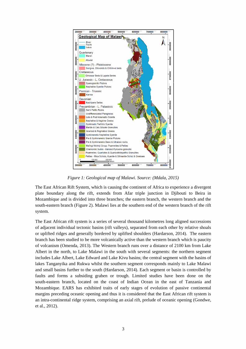
3
Figure 1: Geological map of Malawi. Source: (Mdala, 2015)
The East African Rift System, which is causing the continent of Africa to experience a divergent
plate boundary along the rift, extends from Afar triple junction in Djibouti to Beira in
Mozambique and is divided into three branches; the eastern branch, the western branch and the
south-eastern branch (Figure 2). Malawi lies at the southern end of the western branch of the rift
system.
The East African rift system is a series of several thousand kilometres long aligned successions
of adjacent individual tectonic basins (rift valleys), separated from each other by relative shoals
or uplifted ridges and generally bordered by uplifted shoulders (Hardarson, 2014). The eastern
branch has been studied to be more volcanically active than the western branch which is paucity
of volcanism (Omenda, 2013). The Western branch runs over a distance of 2100 km from Lake
Albert in the north, to Lake Malawi in the south with several segments: the northern segment
includes Lake Albert, Lake Edward and Lake Kivu basins; the central segment with the basins of
lakes Tanganyika and Rukwa whilst the southern segment corresponds mainly to Lake Malawi
and small basins further to the south (Hardarson, 2014). Each segment or basin is controlled by
faults and forms a subsiding graben or trough. Limited studies have been done on the
south-eastern branch, located on the coast of Indian Ocean in the east of Tanzania and
Mozambique. EARS has exhibited traits of early stages of evolution of passive continental
margins preceding oceanic opening and thus it is considered that the East African rift system is
an intra-continental ridge system, comprising an axial rift, prelude of oceanic opening (Gondwe,
et al., 2012).

4
The EARS can therefore be taken as the beginning of opening of an ocean, between two large
continental blocks drifting apart, thus separating the main African plate and the Somalian plate.
The EARS continues to propagate southward at a mean rate between 2.5 cm/year and 5 cm/year
with evidence of seismic activity creating tension and heat (Chorowicz, 2005).
Recent seismic activities experienced on some border faults in Malawi indicate that the
rift-controlling fault system of the Lake Malawi trough is still active (Eliyasi, 2015). Figure 2
shows the East African Rift System.
Figure 2: The East African Rift System. Source (Chorowicz, 2005)
The magnitude of movements on the rift-controlling faults suggests that significant thicknesses
of Neogene deposits could exist in the rift lowlands bordering Lake Malawi, so aquifers may
occur at considerable depth. Geothermal gradients in the EARS vary along the length of the rift
system depending on degree of crustal thinning and volcanic activity (Gondwe, et al., 2012).
The EARS crustal thinning is related to the lithospheric opening that is occurring in the African
continent, which in terms of plate tectonics results from the divergence of large, regional-scale
blocks. The rift is at an early stage of development creating some empty basins, some filled with
sediments of about 3000 m thick and more, while others filled with volcanic rocks with signs of
asthenospheric intrusion (Chorowicz, 2005).
The asthenospheric intrusions in the lithosphere are pronounced along the rift system and are
responsible for negative bouguer anomaly along the rift. However, the intrusion is more
pronouncing in the north and less pronouncing along the line of EARS propagation towards the
5
south where Malawi is. In Afar region, the crust thickness is around 5 km and the region has high
manifestation of geothermal, while moving down south the crust thickness reaches as much as
35 km with sparse geothermal manifestation when compared to the north (Omenda, 2013). The
level of upwelling of the asthenosphere coupled with magmatic bodies close to the earth‘s surface
relates to the level of geothermal gradient along the rift, and this is partly the reason why the
north, i.e. the eastern branch, of the rift system has higher geothermal gradient than the south of
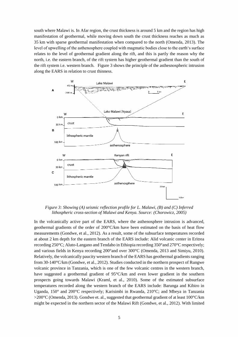
the rift system i.e. western branch. Figure 3 shows the principle of the asthesnospheric intrusion
along the EARS in relation to crust thinness.
Figure 3: Showing (A) seismic reflection profile for L. Malawi, (B) and (C) Inferred
lithospheric cross-section of Malawi and Kenya. Source: (Chorowicz, 2005)
In the volcanically active part of the EARS, where the asthenosphere intrusion is advanced,
geothermal gradients of the order of 200°C/km have been estimated on the basis of heat flow
measurements (Gondwe, et al., 2012). As a result, some of the subsurface temperatures recorded
at about 2 km depth for the eastern branch of the EARS include: Alid volcanic center in Eritrea
recording 250°C; Aluto-Langano and Tendaho in Ethiopia recording 350°and 270°C respectively;
and various fields in Kenya recording 200°and over 300°C (Omenda, 2013 and Simiyu, 2010).
Relatively, the volcanically paucity western branch of the EARS has geothermal gradients ranging
from 30-140°C/km (Gondwe, et al., 2012). Studies conducted in the northern prospect of Rungwe
volcanic province in Tanzania, which is one of the few volcanic centres in the western branch,
have suggested a geothermal gradient of 95°C/km and even lower gradient in the southern
prospects going towards Malawi (Kraml, et al., 2010). Some of the estimated subsurface
temperatures recorded along the western branch of the EARS include: Barunga and Kibiro in
Uganda, 150° and 200°C respectively; Karisimbi in Rwanda, 210°C; and Mbeya in Tanzania
>200°C (Omenda, 2013). Gondwe et. al., suggested that geothermal gradient of at least 100°C/km
might be expected in the northern sector of the Malawi Rift (Gondwe, et al., 2012). With limited
6
studies done to assess the geothermal resource in Malawi, the foregoing concludes that Malawi
system has lower geothermal gradient and hence a medium to low temperature geothermal
system. Detailed studies are however recommended to be more certain of the kind of resource
that Malawi has for appropriate development.
2.1.2. Geothermal manifestation and studies done
Manifestation of geothermal in majority of the sites in Malawi is through hot springs. Studies for
Malawi’s geothermal have been going on for quite a while, however not much details are yet
known about the resource. Most of the studies have concentrated on reconnaissance surveys.
There are over 60 hot springs documented in Malawi with some of them having their water studied
for geochemistry to understand the nature of reservoir, their temperature and the origin of the
water in the system. Most of the work done on the thermal springs focused on mapping litho-
structural control and the physio-chemical characteristics of the hot springs (Dulanya, et al.,
2010). Such studies have revealed that location of the hot springs tend to be along or near the
intersection of major faults within the rift valley, in other words the springs are controlled by the
faults.
The recorded surface temperatures of the hot springs are between 28°C and 79°C (GDC - Kenya,
2010) with some anticipation of beyond 80°C in some cases. Field report submitted to Geological
Surveys Department of Malawi by the Geothermal Development Company of Kenya about the
hot springs’ geochemistry suggests that most of the water are immature and have not attained
equilibrium thereby presenting some degree of uncertainty in geothermometry (GDC - Kenya,
2010). The immaturity of the water may be either as a result of thermal water mixing with ground
fresh water or that the system is permeable and fast recharging. However, subsurface temperature
studies done using sodium potassium (Na-K) geothermometers have indicated a temperature
range of 169⁰ - 249⁰C (GDC - Kenya, 2010). The Na-K geothermometry gives a good indication
for surface exploration that there is a resource in Malawi. However, more study is encouraged to
truly ascertain the details of the resource in terms of actual resource temperature, depth and size
of the resource for appropriate utilization.
The majority of hotter springs in Malawi are located in the northern part of the country and this
includes the most promising field (Chiweta) which records the highest measured surface
temperature. Most of the springs have basic pH signifying that they are weak to affect alteration
in their host rocks. Most of the springs are also overlain by sedimentary rocks thereby the absence
of alteration (Eliyasi, 2015). In tandem with the studies conducted in the western branch of EARS,
utilization of the geothermal resource in this region is suggested through binary electricity power
generation and other direct uses (Hardarson, 2014) due to its low temperature geothermal
gradient.
2.2. Description of Chiweta geothermal field
Located at coordinates 10° 13´S and 34°16´ E at an altitude of about 480 masl, is Chiweta one of
local trading centres in the northern part of Malawi. Chiweta is located within the deep seated
border fault which acts as a conduit for geothermal water (Eliyasi, 2015) and it hosts the hottest
geothermal hot springs recorded so far in Malawi (GDC - Kenya, 2010) which are located to the
immediate north of North Rumphi river, at the edge of Mkerakera hill. Within a distance of 1.5 km
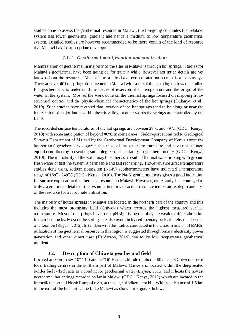
to the east of the hot springs lie Lake Malawi as shown in Figure 4 below.
7
Figure 4: Location of Chiweta hot spring. Source: adapted from (Dulanya, et al., 2010)
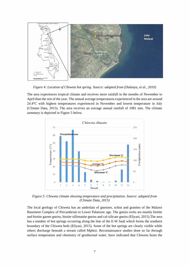
The area experiences tropical climate and receives more rainfall in the months of November to
April than the rest of the year. The annual average temperatures experienced in the area are around
24.4°C with highest temperatures experienced in November and lowest temperature in July
(Climate Data, 2015). The area receives an average annual rainfall of 1081 mm. The climate
summary is depicted in Figure 5 below.
Figure 5: Chiweta climate showing temperature and precipitation. Source: adapted from
(Climate Data, 2015)
The local geology of Chiweta has an underlain of gneisses, schist and granites of the Malawi
Basement Complex of Precambrian to Lower Palaezoic age. The gneiss rocks are mainly biotite
and biotite garnet gneiss, biotite sillimanite gneiss and cal-silicate gneiss (Eliyasi, 2015).The area
has a number of hot springs occurring along the line of the E-W fault which forms the southern
boundary of the Chiweta beds (Eliyasi, 2015). Some of the hot springs are clearly visible while
others discharge beneath a stream called Mphizi. Reconnaissance studies done so far through
surface temperature and chemistry of geothermal water, have indicated that Chiweta hosts the
8
hottest geothermal hot springs recorded in Malawi, with a maximum surface temperature of 79°C
and Na-K geothermometer subsurface temperature of 249°C (GDC - Kenya, 2010).
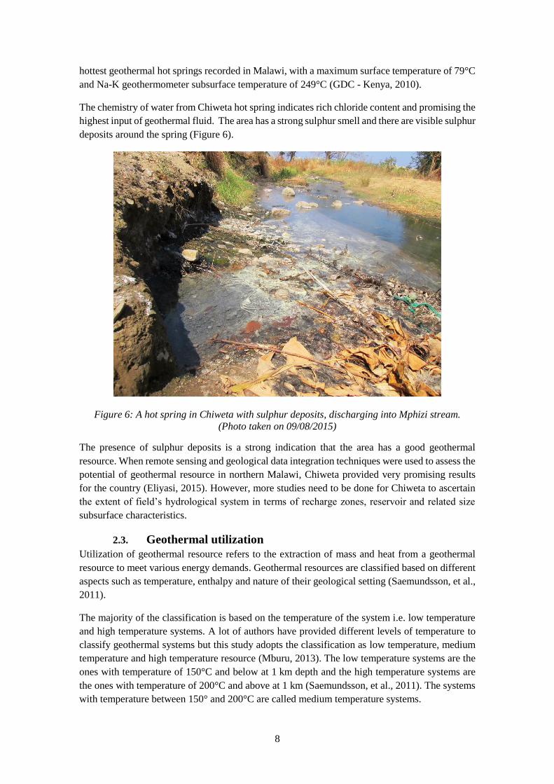
The chemistry of water from Chiweta hot spring indicates rich chloride content and promising the
highest input of geothermal fluid. The area has a strong sulphur smell and there are visible sulphur
deposits around the spring (Figure 6).
Figure 6: A hot spring in Chiweta with sulphur deposits, discharging into Mphizi stream.
(Photo taken on 09/08/2015)
The presence of sulphur deposits is a strong indication that the area has a good geothermal
resource. When remote sensing and geological data integration techniques were used to assess the
potential of geothermal resource in northern Malawi, Chiweta provided very promising results
for the country (Eliyasi, 2015). However, more studies need to be done for Chiweta to ascertain
the extent of field’s hydrological system in terms of recharge zones, reservoir and related size
subsurface characteristics.
2.3. Geothermal utilization
Utilization of geothermal resource refers to the extraction of mass and heat from a geothermal
resource to meet various energy demands. Geothermal resources are classified based on different
aspects such as temperature, enthalpy and nature of their geological setting (Saemundsson, et al.,
2011).
The majority of the classification is based on the temperature of the system i.e. low temperature
and high temperature systems. A lot of authors have provided different levels of temperature to
classify geothermal systems but this study adopts the classification as low temperature, medium
temperature and high temperature resource (Mburu, 2013). The low temperature systems are the
ones with temperature of 150°C and below at 1 km depth and the high temperature systems are
the ones with temperature of 200°C and above at 1 km (Saemundsson, et al., 2011). The systems
with temperature between 150° and 200°C are called medium temperature systems.

9
A summary of classification based on temperature, enthalpy and physical state of a system is
presented in Table 1 below as summarized by Saemundsson et. al (2011).
Table 1: Categories of geothermal systems based on temperature, enthalpy and physical state
(Saemundsson, et al., 2011)
In terms of geological setting, Saemundsson, et. al., (2011) classifies geothermal resources further
as volcanic, convective fracture controlled, sedimentary geo-pressured, hot dry rock also known
as enhanced/engineered geothermal system (EGS), and shallow resources. Of these
classifications, the most commonly encountered geothermal systems are the volcanic systems,
convective and the sedimentary systems and these are defined as follows:
a. Volcanic geothermal system is associated with volcanic activity and the system’s heat
source is hot intrusion or magma. Most of these systems are located at plate
boundaries and some in hot spot areas and the system’s water flow is controlled by
permeable fractures and fault zones.
b. Convective systems have the hot crust at depth as a heat source in tectonically active
areas. In this system, water travel at a considerable depth (> 1 km) through vertical
fractures to mine the heat from the rock.
c. Sedimentary geothermal system have permeable sedimentary layers at depth
(> 1 km) with a geothermal gradient of more than 30°C/km and they are mostly
conductive in nature even though some may be convective.
Most of the high temperature geothermal systems are associated with the volcanic geological
setting while most medium to low temperature systems are associated with convective and
sedimentary geological setting (Saemundsson, et al., 2011).
With the studies done so far, there is not much indication of volcanism for Malawi system which
may determine the system as a high temperature system. As such Malawi is therefore considered
as having a medium to low temperature geothermal system associated with convective or
sedimentary system as evidenced by the presence of limestone and sandstone in its geological
setting. This plays a role in guiding what kind of utilization for the resource would be. However,
more studies on the resource may reveal the real identification of the system.
Low-temperature (LT) systems
with reservoir temperature at
1 km depth below 150°C.
Often characterized by hot or
boiling springs.
Low-enthalpy geothermal
systems with reservoir fluid
enthalpies less than 800
kJ/kg, corresponding to
temperatures less than about
190ºC.
Liquid-dominated geothermal
reservoirs with the water
temperature at, or below, the
boiling point at the prevailing
pressure and the water phase
controls the pressure in the
reservoir. Some steam may be
present.
Medium-temperature (MT)
systems with reservoir
temperature at 1 km depth
between 150- 200°C.
High-temperature (HT)
systems with reservoir
temperature at 1 km depth
above 200°C. Characterized by
fumaroles, steam vents, mud
pools and highly altered ground.
High-enthalpy geothermal
systems with reservoir fluid
enthalpies greater than 800
kJ/kg.
Two-phase geothermal reservoirs
where steam and water co-exist
and the temperature and pressure
follow the boiling point curve.
Vapour-dominated reservoirs
where temperature is at, or above,
boiling at the prevailing pressure
and the steam phase controls the
pressure in the reservoir. Some
liquid water may be present.
10
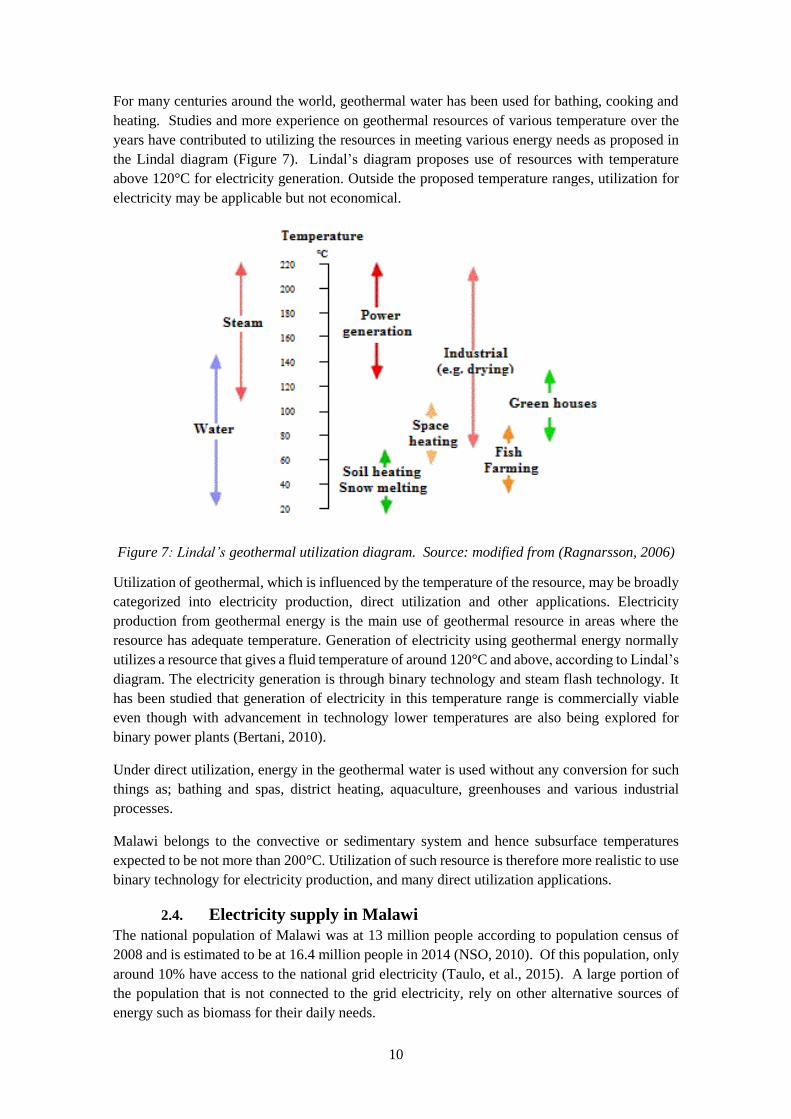
For many centuries around the world, geothermal water has been used for bathing, cooking and
heating. Studies and more experience on geothermal resources of various temperature over the
years have contributed to utilizing the resources in meeting various energy needs as proposed in
the Lindal diagram (Figure 7). Lindal’s diagram proposes use of resources with temperature
above 120°C for electricity generation. Outside the proposed temperature ranges, utilization for
electricity may be applicable but not economical.
Figure 7: Lindal’s geothermal utilization diagram. Source: modified from (Ragnarsson, 2006)
Utilization of geothermal, which is influenced by the temperature of the resource, may be broadly
categorized into electricity production, direct utilization and other applications. Electricity
production from geothermal energy is the main use of geothermal resource in areas where the
resource has adequate temperature. Generation of electricity using geothermal energy normally
utilizes a resource that gives a fluid temperature of around 120°C and above, according to Lindal’s
diagram. The electricity generation is through binary technology and steam flash technology. It
has been studied that generation of electricity in this temperature range is commercially viable
even though with advancement in technology lower temperatures are also being explored for
binary power plants (Bertani, 2010).
Under direct utilization, energy in the geothermal water is used without any conversion for such
things as; bathing and spas, district heating, aquaculture, greenhouses and various industrial
processes.
Malawi belongs to the convective or sedimentary system and hence subsurface temperatures
expected to be not more than 200°C. Utilization of such resource is therefore more realistic to use
binary technology for electricity production, and many direct utilization applications.
2.4. Electricity supply in Malawi
The national population of Malawi was at 13 million people according to population census of
2008 and is estimated to be at 16.4 million people in 2014 (NSO, 2010). Of this population, only
around 10% have access to the national grid electricity (Taulo, et al., 2015). A large portion of
the population that is not connected to the grid electricity, rely on other alternative sources of
energy such as biomass for their daily needs.

11
According to the department of energy affairs, Malawi energy mix is predominantly dependent
on biomass in the form of firewood and charcoal (DoE, 2003). The current status of energy mix
pause a big challenge over the natural vegetation of Malawi as trees are wantonly cut to meet the
energy demand without regard on their sustainability. The Malawi government came up with the
National Energy Policy of 2003 which among others focused on improving efficiency and
effectiveness in energy supply industries and improving security and reliability of energy supply
systems as well as mitigating environmental impacts of energy production and utilization. The
policy wanted to reduce over-dependence of biomass as energy source by increasing energy
supply from other alternative sources (DoE, 2003). Despite having the policy in place, Malawi
has stagnated in developing its alternative sources of energy in general and the electricity sector
in particular, to meet the growing demand.
Malawi has a vertically integrated system of electricity supply industry and the major player of
the industry is the Electricity Supply Corporation of Malawi (ESCOM), a government owned
company. ESCOM owns the hydro power plants in Malawi, transmission lines and distribution
system. The current installed electricity generation capacity for Malawi which is connected to the
national grid is 351 MW (MCC-Malawi, 2015) and this is predominantly generated from hydro,
making over 95% of the total capacity. There are some small scale off grid generators that are not
included in this figure. All the major power stations are located in the southern part of Malawi
along a single river Shire, which runs out of Lake Malawi. The projected maximum demand for
electricity in the year 2014 was at 447 MW (MCC-Malawi, 2015). There has been no additional
electricity generation into the grid this far despite continual connection of new customers onto the
grid in a quest to boost the national access to electricity rate. This means that the electricity
industry is affected by insufficient generation capacity that is failing to satisfy the current
increasing demand. Apart from insufficient generation, poor service quality that comes with
transmission and distribution losses emanating from long transmission distances, ageing
equipment as well as environmental effects, affect the operations of the hydro power plants to the
effect of reducing power production capacity further affecting the delivery of electricity. Because
of these problems, customers are subjected to power rationing where load-shedding programmes
are the order of the day as the utility company manages the electricity supply. This kind of
electricity supply negatively affects the economic activities in the country.
With the erratic supply of electricity that the country experiences coupled with will development
of electricity supply projects, the country’s dependence on biomass may be higher than the
currently projected as presented in Table 2.
Table 2: Energy Mix Projections 2000 – 2050. Source: adapted from DoE (2003)
Energy source 2000 2010 2020 2050
Biomass 93 % 75 % 50 % 30 %
Liquid Fuels 3.5 % 5.5 % 7 % 10 %
Electricity (hydro) 2.3 % 10 % 30 % 40 %
Coal 1 % 4 % 6 % 6 %
Renewables 0.2 % 5.5 % 7 % 10 %
Nuclear 0 % 0 % 0 % 4 %
TOTAL 100% 100% 100% 100%

12
Malawi has one of the lowest electricity consumption per capita in the world which stands around
93kWh (Taulo, et al., 2015). With this fact, the country stands below the recommended
sub-Saharan electricity consumption per capita rate of 432kWh, let alone the world’s
recommended average per capita rate of 2167kWh (Taulo, et al., 2015). This means the country
needs more energy projects to improve on its per capita consumption, which in a way assists in
improving the living standards of the people.
With the electricity challenges being faced by the country and the desire to provide affordable
and clean energy for the populace, it has become imperative for the country to review and assess
the role of alternative sources of energy for the country to boost its energy capacity. The
Department of Energy Affairs has embarked on a process of reviewing the energy policy in order
to have a policy that is responsive to the prevailing energy ills. The reviewed policy is expected
to incorporate various potential alternative energy sources in Malawi that would in one way or
the other provide lasting solutions to the energy problems. Amongst the potential candidates,
geothermal power technology is being considered for development that would assist in meeting
the growing energy demand of the country. Being in the western branch of the EARS, this study
therefore focuses on designing a binary cycle for Malawi’s Chiweta geothermal resource that the
country may adopt for development.
13
3.0. Geothermal power plant technologies Geothermal power plants are divided into two main categories: the steam cycle power plants and
binary cycle power plants (Valdimarsson, 2010). Steam power plants convert thermal energy
from geothermal fluid to electricity by letting the fluid boil (flashing), or using dry steam directly
from the resource where the resource has the capacity to produce steam. Binary cycle power plants
generally utilize the geothermal fluid in liquid form, without flashing, to produce electricity. Some
binary plants are coupled to a steam flash cycle (hybrid) to use the exhaust heat from the flash
plant thereby improving cycle thermal efficiency of the entire system. Binary plants use two
cycles with different fluids, the geothermal fluid in one cycle as a source of heat, and an organic
fluid in the other cycle.
The two categories of power plants are further divided into various sub-types of power plants.
For steam cycle plants, these include: Single flash steam plants, double flash steam plant, and
cascaded flash plants. For binary or Organic Rankine Cycle (ORC), there is the ordinary binary
plant and the Kalina cycle. There is also a combination of flash plant with an ORC plant which
sometimes is called hybrid plant. Application of a type of power plant technology mostly depends
on specific characteristics of a given geothermal field in terms of resource temperature vis-à-vis
enthalpy, and whether the field is steam dominated or liquid dominated. The power plant
categories are discussed further below.
3.1. Steam flash power plants
In steam flash plant it is assumed that the geothermal fluid is a compressed liquid from the
reservoir. The common assumption is based on the fact that generally dry steam reservoirs are
very rare (DiPippo, 1999). Where vapour dominated reservoirs exist, direct-steam plants are used,
and otherwise the assumption holds.
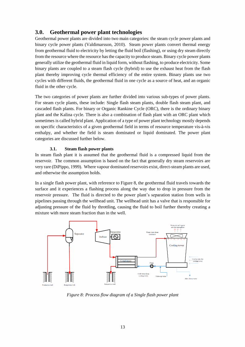
In a single flash power plant, with reference to Figure 8, the geothermal fluid travels towards the
surface and it experiences a flashing process along the way due to drop in pressure from the
reservoir pressure. The fluid is directed to the power plant’s separation station from wells in
pipelines passing through the wellhead unit. The wellhead unit has a valve that is responsible for
adjusting pressure of the fluid by throttling, causing the fluid to boil further thereby creating a
mixture with more steam fraction than in the well.
Figure 8: Process flow diagram of a Single flash power plant
14
The steam is expanded through the turbine thereby providing a mechanical force that drives the
turbine. The turbine is coupled to a generator that eventually generates electricity as the steam is
being expanded through the turbine.
After passing through the turbine, the steam is either released into the environment in a case of a
back-pressure power plant, or it is sent to a cooling system through a hot well in a case of a
condensing steam power plant. The condensate is then either directed to reinjection wells or may
be used as make up water in the power plant’s cooling system.
The brine from the separator, which is not required to flash further, is directed to reinjection wells
or directed for other utilization such as district heating where the chemistry allows. A typical
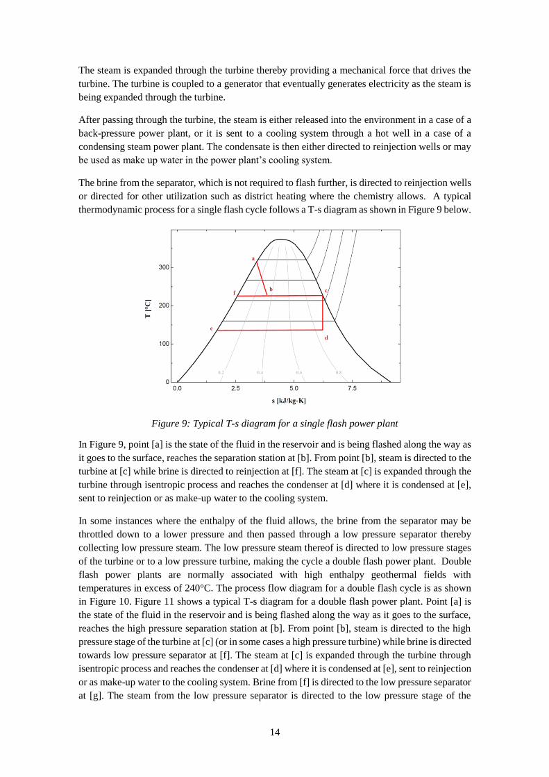
thermodynamic process for a single flash cycle follows a T-s diagram as shown in Figure 9 below.
Figure 9: Typical T-s diagram for a single flash power plant
In Figure 9, point [a] is the state of the fluid in the reservoir and is being flashed along the way as
it goes to the surface, reaches the separation station at [b]. From point [b], steam is directed to the
turbine at [c] while brine is directed to reinjection at [f]. The steam at [c] is expanded through the
turbine through isentropic process and reaches the condenser at [d] where it is condensed at [e],
sent to reinjection or as make-up water to the cooling system.
In some instances where the enthalpy of the fluid allows, the brine from the separator may be
throttled down to a lower pressure and then passed through a low pressure separator thereby
collecting low pressure steam. The low pressure steam thereof is directed to low pressure stages
of the turbine or to a low pressure turbine, making the cycle a double flash power plant. Double
flash power plants are normally associated with high enthalpy geothermal fields with
temperatures in excess of 240°C. The process flow diagram for a double flash cycle is as shown
in Figure 10. Figure 11 shows a typical T-s diagram for a double flash power plant. Point [a] is
the state of the fluid in the reservoir and is being flashed along the way as it goes to the surface,
reaches the high pressure separation station at [b]. From point [b], steam is directed to the high
pressure stage of the turbine at [c] (or in some cases a high pressure turbine) while brine is directed
towards low pressure separator at [f]. The steam at [c] is expanded through the turbine through
isentropic process and reaches the condenser at [d] where it is condensed at [e], sent to reinjection
or as make-up water to the cooling system. Brine from [f] is directed to the low pressure separator
at [g]. The steam from the low pressure separator is directed to the low pressure stage of the
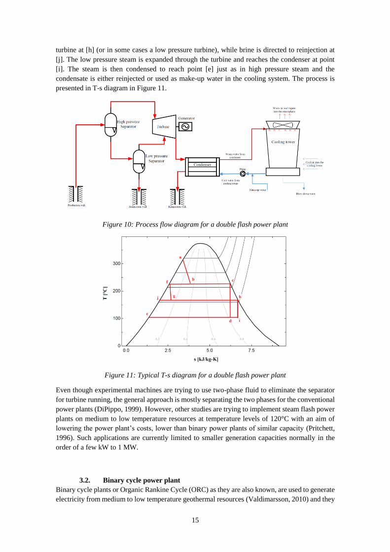
15
turbine at [h] (or in some cases a low pressure turbine), while brine is directed to reinjection at
[j]. The low pressure steam is expanded through the turbine and reaches the condenser at point
[i]. The steam is then condensed to reach point [e] just as in high pressure steam and the
condensate is either reinjected or used as make-up water in the cooling system. The process is
presented in T-s diagram in Figure 11.
Figure 10: Process flow diagram for a double flash power plant
Figure 11: Typical T-s diagram for a double flash power plant
Even though experimental machines are trying to use two-phase fluid to eliminate the separator
for turbine running, the general approach is mostly separating the two phases for the conventional
power plants (DiPippo, 1999). However, other studies are trying to implement steam flash power
plants on medium to low temperature resources at temperature levels of 120°C with an aim of
lowering the power plant’s costs, lower than binary power plants of similar capacity (Pritchett,
1996). Such applications are currently limited to smaller generation capacities normally in the
order of a few kW to 1 MW.
3.2. Binary cycle power plant
Binary cycle plants or Organic Rankine Cycle (ORC) as they are also known, are used to generate
electricity from medium to low temperature geothermal resources (Valdimarsson, 2010) and they
16
help to increase efficiency of geothermal fluid through recovery of heat from waste fluid of steam
flash power plants. Binary power plants use a secondary working fluid, which is organic, to
produce electricity. The secondary working fluid has a low boiling point and a high vapour
pressure at low temperatures when compared to water (Maghiar & Antal, 2001).
The optimal temperature range for utilizing binary power plants varies from author to author.
Some have given a temperature range of 85° - 170°C (Maghiar & Antal, 2001), others a range of
120° - 190°C (Eliasson, et al., 2008) while yet others a range of 100°- 220°C (Hettiarachchi, et
al., 2007). This work therefore considers that an optimal temperature range for binary application
is 85°- 220°C. When a binary cycle is applied for a field with temperature above the upper
temperature limit, there are issues of thermal stability with the organic fluids (Maghiar & Antal,
2001). On the other side, applying the binary cycle in the lower temperature limit becomes
impractical and uneconomical. At low temperature, the heat exchanger size for a given capacity
becomes impractical and the parasitic loads requires a large percentage of the power generated.
The medium to low temperature geothermal resources are in abundance worldwide and this makes
the use of binary power plants to be popular in electricity generation applications for geothermal
utilization.
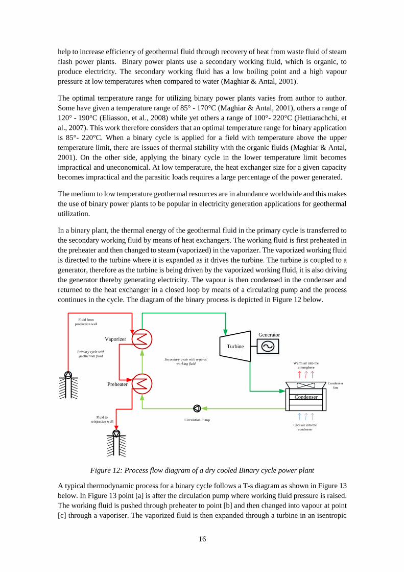
In a binary plant, the thermal energy of the geothermal fluid in the primary cycle is transferred to
the secondary working fluid by means of heat exchangers. The working fluid is first preheated in
the preheater and then changed to steam (vaporized) in the vaporizer. The vaporized working fluid
is directed to the turbine where it is expanded as it drives the turbine. The turbine is coupled to a
generator, therefore as the turbine is being driven by the vaporized working fluid, it is also driving
the generator thereby generating electricity. The vapour is then condensed in the condenser and
returned to the heat exchanger in a closed loop by means of a circulating pump and the process
continues in the cycle. The diagram of the binary process is depicted in Figure 12 below.
Figure 12: Process flow diagram of a dry cooled Binary cycle power plant
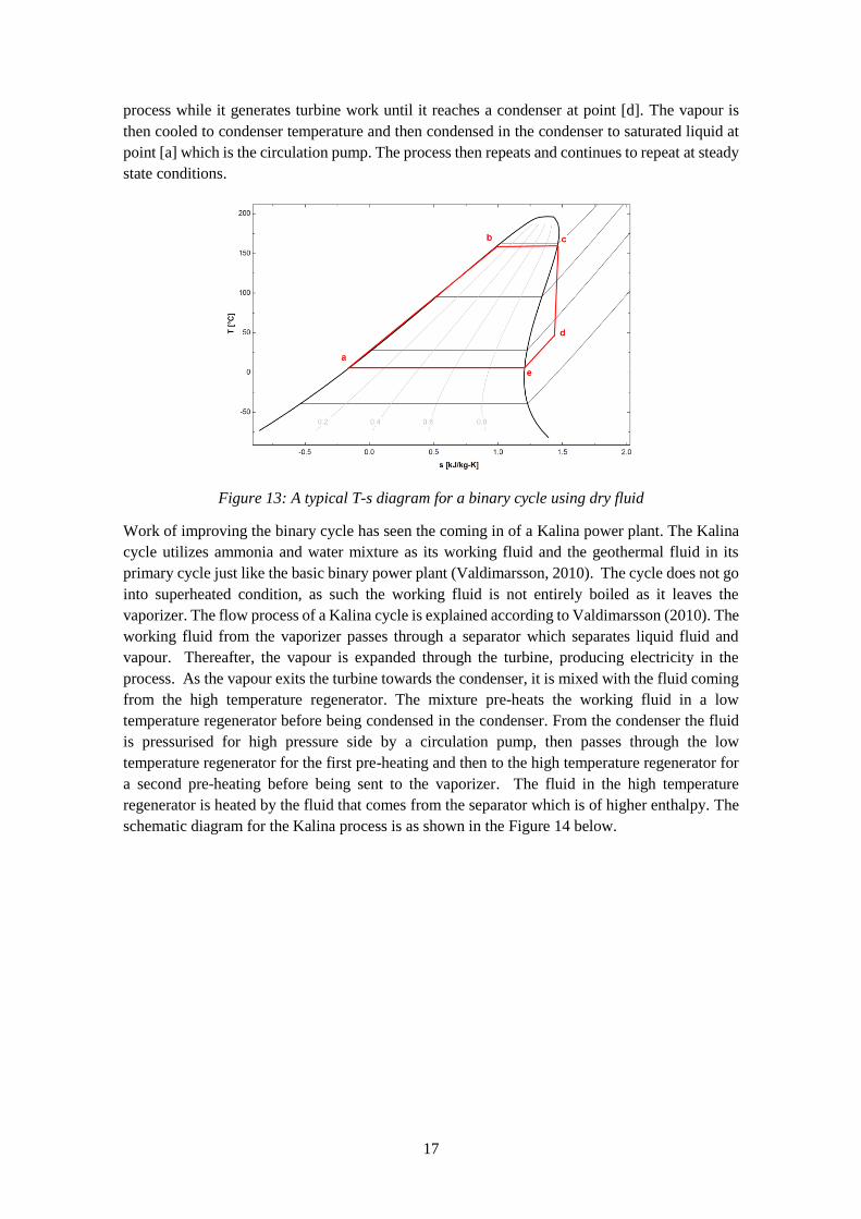
A typical thermodynamic process for a binary cycle follows a T-s diagram as shown in Figure 13
below. In Figure 13 point [a] is after the circulation pump where working fluid pressure is raised.
The working fluid is pushed through preheater to point [b] and then changed into vapour at point
[c] through a vaporiser. The vaporized fluid is then expanded through a turbine in an isentropic
Fluid from
production well
Vaporizer
Preheater
Circulation Pump
Turbine
Generator
Fluid to
reinjection well
Secondary cycle with organic
working fluid
Primary cycle with
geothermal fluid
Cool air into the
condenser
Warm air into the
atmosphere
Condenser
fan
Condenser
17
process while it generates turbine work until it reaches a condenser at point [d]. The vapour is
then cooled to condenser temperature and then condensed in the condenser to saturated liquid at
point [a] which is the circulation pump. The process then repeats and continues to repeat at steady
state conditions.
Figure 13: A typical T-s diagram for a binary cycle using dry fluid
Work of improving the binary cycle has seen the coming in of a Kalina power plant. The Kalina
cycle utilizes ammonia and water mixture as its working fluid and the geothermal fluid in its
primary cycle just like the basic binary power plant (Valdimarsson, 2010). The cycle does not go
into superheated condition, as such the working fluid is not entirely boiled as it leaves the
vaporizer. The flow process of a Kalina cycle is explained according to Valdimarsson (2010). The
working fluid from the vaporizer passes through a separator which separates liquid fluid and
vapour. Thereafter, the vapour is expanded through the turbine, producing electricity in the
process. As the vapour exits the turbine towards the condenser, it is mixed with the fluid coming
from the high temperature regenerator. The mixture pre-heats the working fluid in a low
temperature regenerator before being condensed in the condenser. From the condenser the fluid
is pressurised for high pressure side by a circulation pump, then passes through the low
temperature regenerator for the first pre-heating and then to the high temperature regenerator for
a second pre-heating before being sent to the vaporizer. The fluid in the high temperature
regenerator is heated by the fluid that comes from the separator which is of higher enthalpy. The
schematic diagram for the Kalina process is as shown in the Figure 14 below.
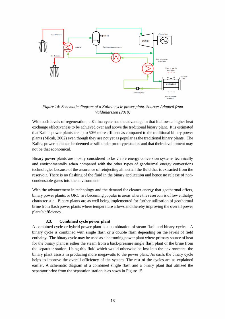
18
Figure 14: Schematic diagram of a Kalina cycle power plant. Source: Adapted from
Valdimarsson (2010)
With such levels of regeneration, a Kalina cycle has the advantage in that it allows a higher heat
exchange effectiveness to be achieved over and above the traditional binary plant. It is estimated
that Kalina power plants are up to 50% more efficient as compared to the traditional binary power
plants (Mlcak, 2002) even though they are not yet as popular as the traditional binary plants. The
Kalina power plant can be deemed as still under prototype studies and that their development may
not be that economical.
Binary power plants are mostly considered to be viable energy conversion systems technically
and environmentally when compared with the other types of geothermal energy conversions
technologies because of the assurance of reinjecting almost all the fluid that is extracted from the
reservoir. There is no flashing of the fluid in the binary application and hence no release of non-
condensable gases into the environment.
With the advancement in technology and the demand for cleaner energy that geothermal offers,
binary power plants, or ORC, are becoming popular in areas where the reservoir is of low enthalpy
characteristic. Binary plants are as well being implemented for further utilization of geothermal
brine from flash power plants where temperature allows and thereby improving the overall power
plant’s efficiency.
3.3. Combined cycle power plant A combined cycle or hybrid power plant is a combination of steam flash and binary cycles. A
binary cycle is combined with single flash or a double flash depending on the levels of field
enthalpy. The binary cycle may be used as a bottoming power plant where primary source of heat
for the binary plant is either the steam from a back-pressure single flash plant or the brine from
the separator station. Using this fluid which would otherwise be lost into the environment, the
binary plant assists in producing more megawatts to the power plant. As such, the binary cycle
helps to improve the overall efficiency of the system. The rest of the cycles are as explained
earlier. A schematic diagram of a combined single flash and a binary plant that utilized the
separator brine from the separation station is as sown in Figure 15.

19
Figure 15: Combined single flash and binary power plant
A suitable power plant design for any field is supposed to match with the field’s parameters in
terms of enthalpy, mass flow and chemistry, at the same time it is supposed to be reliable and
environmentally friendly while being economically viable. Previous studies based on the
geochemistry data available for Malawi, indicated that Malawi may develop its geothermal
resource through single flash power plant, binary power plant or hybrid of single flash and binary
cycle power plant with an emphasis on the combined cycle (Mwagomba, 2013). However, with
limited data available, it is extremely difficult to be certain that Malawi would develop a single
flash plant. Howbeit, basing on the knowledge of power plants and the little information on
Malawi coupled with the facts of the western branch of the EARS where Malawi belongs, it can
be proposed that Malawi would develop a modular binary power plant as the most suitable power
plant for the Chiweta field. As the power plant is developed and being utilized, more information
about the field will be gathered and adjustments to the model of the power plant would be effected
along the way thereby providing a probability of scaling the production capacity of the field.
The analysis of the proposed cycles is presented in the following sections regarding the
assessments in terms of both technical and economic feasibility.
Production well
Separator
Condenser
Flash
Turbine
Flash Generator
Reinjection well
Vaporizer
Preheater
Circulation Pump
Binary
Turbine
Binary
Generator
Reinjection well
Secondary cycle with organic
working fluid
Primary cycle with separator brine
Make-up water
Blow down water
Cooling tower
Condenser
Cold air into the condenser
Warm air out of the
condenser
Warm air out of the cooling
tower
Cold air into the
cooling tower
Pump

20
4.0. Technical analysis of the technology applicable for Chiweta
system The geothermal resources in Malawi are currently used for direct application mainly for bathing.
Hot springs in Nkhotakota, with surface temperature of around 72°C (GDC - Kenya, 2010), were
once used for district heating at a local hospital during winter periods showing that direct
utilization of geothermal in Malawi is possible. This study however focuses on electricity
generation.
There are a number of factors that are considered for extraction of energy from a geothermal
resource some of which are the reservoir capacity, temperature of the resource, mass flow of the
fluid and the chemistry of the fluid. Not much study has been done on Malawi’s geothermal to
ascertain reservoir parameters. Malawi needs to do detailed assessment of its geothermal resource
to the point of drilling exploration wells in order to be certain of the said parameters.
This study therefore uses the surface data available and educated estimates wherever necessary,
to give the resource parameters for modelling and improve the certainty of implementation. The
proposed binary plant would be modular with provision for further capacity upgrade. Modular
development of binary power plants is cost effective and facilitates short manufacturing and
installation times and can be upgraded to as much as 50MW (Maghiar & Antal, 2001).
As the binary power plant will be operated, more data of the field will be obtained to fine tune
initial reservoir parameters which will guide further exploration and developments. The
temperature of the resource is as guided by the various studies done in the area.
4.1. Thermodynamic analysis
The binary power plant will have two fluid circulation systems for generation of electricity i.e.
the primary and the secondary systems. The primary circulating system, which is the heat source
for the cycle, will use the hot geothermal water which is the energy source. The secondary system
is a closed loop using working fluid with low boiling point and high vapour pressure as compared
to water at a common given temperature. The working fluid will get its heat from the hot
geothermal fluid from the primary system by means of heat exchangers. The cycle is cooled by a
cooling system that is coupled to the cycle’s condenser. The primary cycle is designated with a
subscript (s) in all parameters concerned. The secondary cycle and the cooling cycle are
designated with subscripts (wf) and (c) respectively.
The thermodynamic analysis of the binary power plant is based on the schematic diagram in
Figure 12. Hot geothermal water comes from production well and is directed to heat exchangers.
The heat from the geothermal water is transferred to a secondary working fluid through the heat
exchangers in the preheater and vaporizer after which the geothermal water is sent back into the
reservoir through a reinjection well.
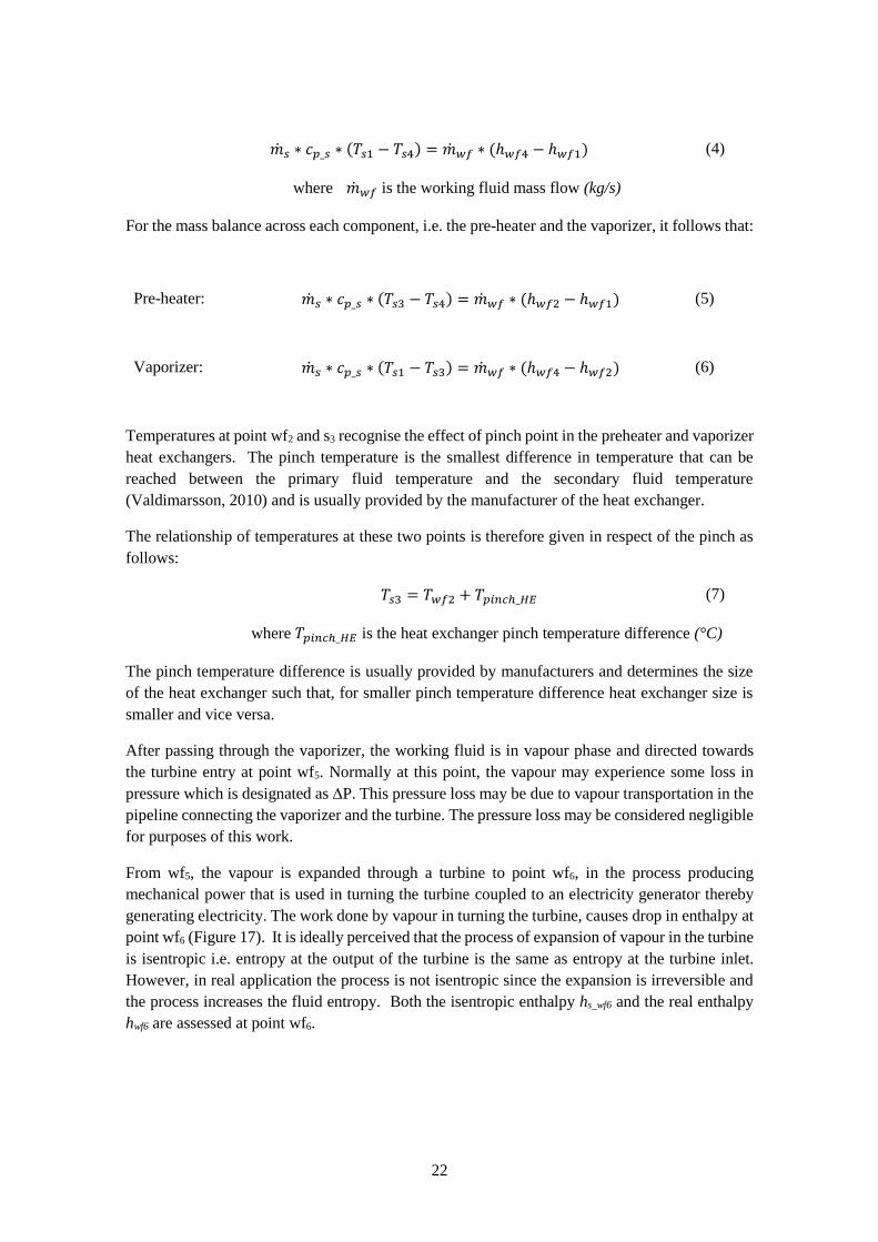
The geothermal fluid enters the primary cycle at point s1, vaporizes the working fluid and
superheats the fluid at point s2 in the vaporizer. The geothermal fluid then leaves the vaporizer
and enters the pre-heater through point s3. The geothermal fluid heats the working fluid in the
pre-heater and leaves the pre-heater through point s4 for reinjection (Figure 16).
For the working fluid in the secondary cycle, the working fluid enters the pre-heater through point
wf1 and is heated by the geothermal fluid. The working fluid leaves the pre-heater and enters the
vaporizer through point wf2. In the vaporizer the fluid is changed to vapour and then superheated
21
at point wf3. The working fluid leaves the vaporizer through point wf4 as superheated vapour
where it is directed towards the turbine (Figure 16).
Figure 16: Vaporizer and preheater section of the binary cycle
The process of vaporizer and preheater heat exchange is in such a way that the heat rejected by
the geothermal fluid is received by the working fluid. The thermodynamic assessment is therefore
as follows:
�̇�𝑠 = �̇�𝑤𝑓 (kJ/s) (1)
where �̇�𝑠 is the total heat rejected by geothermal fluid
�̇�𝑤𝑓 is the total heat received by the working fluid.
Total heat rejected by the geothermal fluid is the sum of heat rejected by the geothermal fluid in
both the vaporizer and the pre-heater and is given by the equation as follows:
�̇�𝑠 = �̇�𝑠 ∗ (ℎ𝑠1 − ℎ𝑠4) (kJ/s) (2)
where �̇�𝑠 is the geothermal fluid mass flow (kg/s)
ℎ𝑠𝑥 is the source enthalpy at point x (kJ/kg)
If temperatures and heat capacity are used instead of enthalpy, equation (2) becomes:
�̇�𝑠 = �̇�𝑠 ∗ 𝑐𝑝_𝑠 ∗ (𝑇𝑠1 − 𝑇𝑠4) (kJ/s) (3)
where 𝑐𝑝_𝑠 is the geo fluid specific heat capacity (kJ/kg-°C)
𝑇𝑠𝑥 is the source temperature at point x (°C)
Since all the heat rejected by the geothermal fluid is received by the working fluid, the mass
balance across the primary and secondary cycle in the vaporizer and preheater then becomes:
s1
s3
s4 wf1
Vaporizer
Preheater
s2
wf2
wf3
wf4
22
�̇�𝑠 ∗ 𝑐𝑝_𝑠 ∗ (𝑇𝑠1 − 𝑇𝑠4) = �̇�𝑤𝑓 ∗ (ℎ𝑤𝑓4 − ℎ𝑤𝑓1) (4)
where �̇�𝑤𝑓 is the working fluid mass flow (kg/s)
For the mass balance across each component, i.e. the pre-heater and the vaporizer, it follows that:
Pre-heater: �̇�𝑠 ∗ 𝑐𝑝_𝑠 ∗ (𝑇𝑠3 − 𝑇𝑠4) = �̇�𝑤𝑓 ∗ (ℎ𝑤𝑓2 − ℎ𝑤𝑓1)
(5)
Vaporizer: �̇�𝑠 ∗ 𝑐𝑝_𝑠 ∗ (𝑇𝑠1 − 𝑇𝑠3) = �̇�𝑤𝑓 ∗ (ℎ𝑤𝑓4 − ℎ𝑤𝑓2)
(6)
Temperatures at point wf2 and s3 recognise the effect of pinch point in the preheater and vaporizer
heat exchangers. The pinch temperature is the smallest difference in temperature that can be
reached between the primary fluid temperature and the secondary fluid temperature
(Valdimarsson, 2010) and is usually provided by the manufacturer of the heat exchanger.
The relationship of temperatures at these two points is therefore given in respect of the pinch as
follows:
𝑇𝑠3 = 𝑇𝑤𝑓2 + 𝑇𝑝𝑖𝑛𝑐ℎ_𝐻𝐸 (7)
where 𝑇𝑝𝑖𝑛𝑐ℎ_𝐻𝐸 is the heat exchanger pinch temperature difference (°C)
The pinch temperature difference is usually provided by manufacturers and determines the size
of the heat exchanger such that, for smaller pinch temperature difference heat exchanger size is
smaller and vice versa.
After passing through the vaporizer, the working fluid is in vapour phase and directed towards
the turbine entry at point wf5. Normally at this point, the vapour may experience some loss in
pressure which is designated as ∆P. This pressure loss may be due to vapour transportation in the
pipeline connecting the vaporizer and the turbine. The pressure loss may be considered negligible
for purposes of this work.
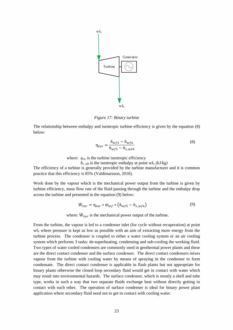
From wf5, the vapour is expanded through a turbine to point wf6, in the process producing
mechanical power that is used in turning the turbine coupled to an electricity generator thereby
generating electricity. The work done by vapour in turning the turbine, causes drop in enthalpy at
point wf6 (Figure 17). It is ideally perceived that the process of expansion of vapour in the turbine
is isentropic i.e. entropy at the output of the turbine is the same as entropy at the turbine inlet.
However, in real application the process is not isentropic since the expansion is irreversible and
the process increases the fluid entropy. Both the isentropic enthalpy hs_wf6 and the real enthalpy
hwf6 are assessed at point wf6.
23
Figure 17: Binary turbine
The relationship between enthalpy and isentropic turbine efficiency is given by the equation (8)
below:
ɳ𝑡𝑢𝑟 =
ℎ𝑤𝑓5 − ℎ𝑤𝑓6
ℎ𝑤𝑓5 − ℎ𝑠_𝑤𝑓6
(8)
where: ɳtur is the turbine isentropic efficiency
hs_wf6 is the isentropic enthalpy at point wf6 (kJ/kg)
The efficiency of a turbine is generally provided by the turbine manufacturer and it is common
practice that this efficiency is 85% (Valdimarsson, 2010).
Work done by the vapour which is the mechanical power output from the turbine is given by
turbine efficiency, mass flow rate of the fluid passing through the turbine and the enthalpy drop
across the turbine and presented in the equation (9) below:
Ẇ𝑡𝑢𝑟 = ɳ𝑡𝑢𝑟 ∗ ṁ𝑤𝑓 ∗ (ℎ𝑤𝑓5 − ℎ𝑠_𝑤𝑓6) (9)
where: Ẇ𝑡𝑢𝑟 is the mechanical power output of the turbine.
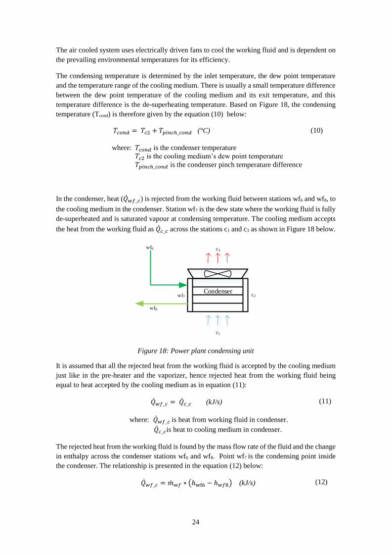
From the turbine, the vapour is led to a condenser inlet (for cycle without recuperation) at point
wf6 where pressure is kept as low as possible with an aim of extracting more energy from the
turbine process. The condenser is coupled to either a water cooling system or an air cooling
system which performs 3 tasks: de-superheating, condensing and sub-cooling the working fluid.
Two types of water cooled condensers are commonly used in geothermal power plants and these
are the direct contact condenser and the surface condenser. The direct contact condensers mixes
vapour from the turbine with cooling water by means of spraying in the condenser to form
condensate. The direct contact condenser is applicable in flash plants but not appropriate for
binary plants otherwise the closed loop secondary fluid would get in contact with water which
may result into environmental hazards. The surface condenser, which is mostly a shell and tube
type, works in such a way that two separate fluids exchange heat without directly getting in
contact with each other. The operation of surface condenser is ideal for binary power plant
application where secondary fluid need not to get in contact with cooling water.
Turbine
Generator
wf5
wf6
24
The air cooled system uses electrically driven fans to cool the working fluid and is dependent on
the prevailing environmental temperatures for its efficiency.
The condensing temperature is determined by the inlet temperature, the dew point temperature
and the temperature range of the cooling medium. There is usually a small temperature difference
between the dew point temperature of the cooling medium and its exit temperature, and this
temperature difference is the de-superheating temperature. Based on Figure 18, the condensing
temperature (Tcond) is therefore given by the equation (10) below:
𝑇𝑐𝑜𝑛𝑑 = 𝑇𝑐2 + 𝑇𝑝𝑖𝑛𝑐ℎ_𝑐𝑜𝑛𝑑 (°C) (10)
where: 𝑇𝑐𝑜𝑛𝑑 is the condenser temperature
𝑇𝑐2 is the cooling medium’s dew point temperature
𝑇𝑝𝑖𝑛𝑐ℎ_𝑐𝑜𝑛𝑑 is the condenser pinch temperature difference
In the condenser, heat (�̇�𝑤𝑓_𝑐) is rejected from the working fluid between stations wf6 and wf8, to
the cooling medium in the condenser. Station wf7 is the dew state where the working fluid is fully
de-superheated and is saturated vapour at condensing temperature. The cooling medium accepts
the heat from the working fluid as �̇�𝑐_𝑐 across the stations c1 and c3 as shown in Figure 18 below.
Figure 18: Power plant condensing unit
It is assumed that all the rejected heat from the working fluid is accepted by the cooling medium
just like in the pre-heater and the vaporizer, hence rejected heat from the working fluid being
equal to heat accepted by the cooling medium as in equation (11):
�̇�𝑤𝑓_𝑐 = �̇�𝑐_𝑐 (kJ/s) (11)
where: �̇�𝑤𝑓_𝑐 is heat from working fluid in condenser.
�̇�𝑐_𝑐is heat to cooling medium in condenser.
The rejected heat from the working fluid is found by the mass flow rate of the fluid and the change
in enthalpy across the condenser stations wf6 and wf8. Point wf7 is the condensing point inside
the condenser. The relationship is presented in the equation (12) below:
�̇�𝑤𝑓_𝑐 = �̇�𝑤𝑓 ∗ (ℎwf6 − ℎ𝑤𝑓8) (kJ/s) (12)
wf7
Condenser
wf6
c1
c3
wf8
c2
25
�̇�𝑐𝑤 is found by multiplying the cooling fluid mass flow rate and the change in enthalpy in the
cooling water across the condenser as given in the equation (13) below:
�̇�𝑐_𝑐 = �̇�𝑐 ∗ (ℎ𝑐3 − ℎ𝑐1) (kJ/s) (13)
where: hcx is cooling fluid enthalpy at point x.
�̇�𝑐 is the cooling fluid mass flow.
When temperatures at stations c1 and c3 are used, the equation becomes:
�̇�𝑐𝑤 = �̇�𝑐 ∗ 𝐶𝑝𝑐∗ (𝑇𝑐3 − 𝑇𝑐1) (kJ/s) (14)
where: 𝐶𝑝_𝑐 is the specific heat capacity for cooling fluid.
Tcx is the cooling fluid temperature at point x.
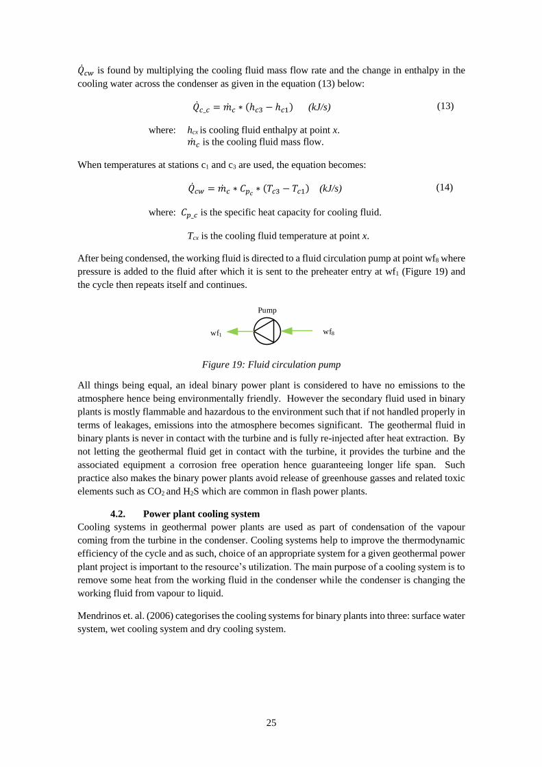
After being condensed, the working fluid is directed to a fluid circulation pump at point wf8 where
pressure is added to the fluid after which it is sent to the preheater entry at wf1 (Figure 19) and
the cycle then repeats itself and continues.
Figure 19: Fluid circulation pump
All things being equal, an ideal binary power plant is considered to have no emissions to the
atmosphere hence being environmentally friendly. However the secondary fluid used in binary
plants is mostly flammable and hazardous to the environment such that if not handled properly in
terms of leakages, emissions into the atmosphere becomes significant. The geothermal fluid in
binary plants is never in contact with the turbine and is fully re-injected after heat extraction. By
not letting the geothermal fluid get in contact with the turbine, it provides the turbine and the
associated equipment a corrosion free operation hence guaranteeing longer life span. Such
practice also makes the binary power plants avoid release of greenhouse gasses and related toxic
elements such as CO2 and H2S which are common in flash power plants.
4.2. Power plant cooling system
Cooling systems in geothermal power plants are used as part of condensation of the vapour
coming from the turbine in the condenser. Cooling systems help to improve the thermodynamic
efficiency of the cycle and as such, choice of an appropriate system for a given geothermal power
plant project is important to the resource’s utilization. The main purpose of a cooling system is to
remove some heat from the working fluid in the condenser while the condenser is changing the
working fluid from vapour to liquid.
Mendrinos et. al. (2006) categorises the cooling systems for binary plants into three: surface water
system, wet cooling system and dry cooling system.
Pump
wf8wf1

26
4.2.1. Surface water system
The surface water system which is also known as once-through cooling system, removes heat
from the condenser by using water, passing the water through the condenser and releasing the
water into the environment thereafter. This type of cooling system is able to yield the lowest
condensing temperature thereby improving the significantly the thermodynamic efficiency of the
cycle as compared to the other cooling systems (Mendrinos, et al., 2006). The technology does
not require cooling towers as in the case of the two systems to be discussed below, because the
water used in cooling system are discharged into the environment once they have been used in
the condenser. The analysis of the cooling system is basically the heat exchange in the condenser
using equation (14). The heat in the working fluid is rejected to the cooling water as the cooling
water passes through the condenser. Mass balance and enthalpies are calculated based on
equations (12) and (14) to ascertain the quantity of water required for the system at the ambient
water temperature and the desired condenser temperature. The system requires a considerably
large and steady source of water body for its satisfactory operation and the water requirements in
this system are almost 30 times as much as those required in a wet cooling system. Despite its
standing on thermal efficiency improvement, the technology is not popular due to the large
volume of water that are required in light of other water demands, water rights, and related water
issues. The system results in increase in the water body’s temperature thereby affecting the
ecosystem in the water body. However, where water is not an issue and the quality of water is
studied with an aim of preserving the condenser, implementation of surface water cooling system
is recommended. This study however will not consider the surface water cooling system in its
further analyses that follow.
4.2.2. Wet cooling system
Wet cooling system uses both water and air with a cooling tower that may be configured as cross
flow or counter flow depending on the direction of air entering the cooling tower. The water from
the cooling system is let to pass through the condenser where it removes heat from the working
fluid. This water then directed to the top of the cooling tower where the heat is rejected into the
environment by action of air. The water is collected at the bottom of the tower to remove the heat
again from the working fluid in the condenser. The system requires considerably large amounts
of water but not as much as in the surface water cooling system. Some of the cooling water may
be lost in the process at the cooling tower presenting a requirement of a steady and abundant
supply of fresh water to be used as make-up water for the system. A schematic diagram for a wet
cooling system is as shown in Figure 20 below.
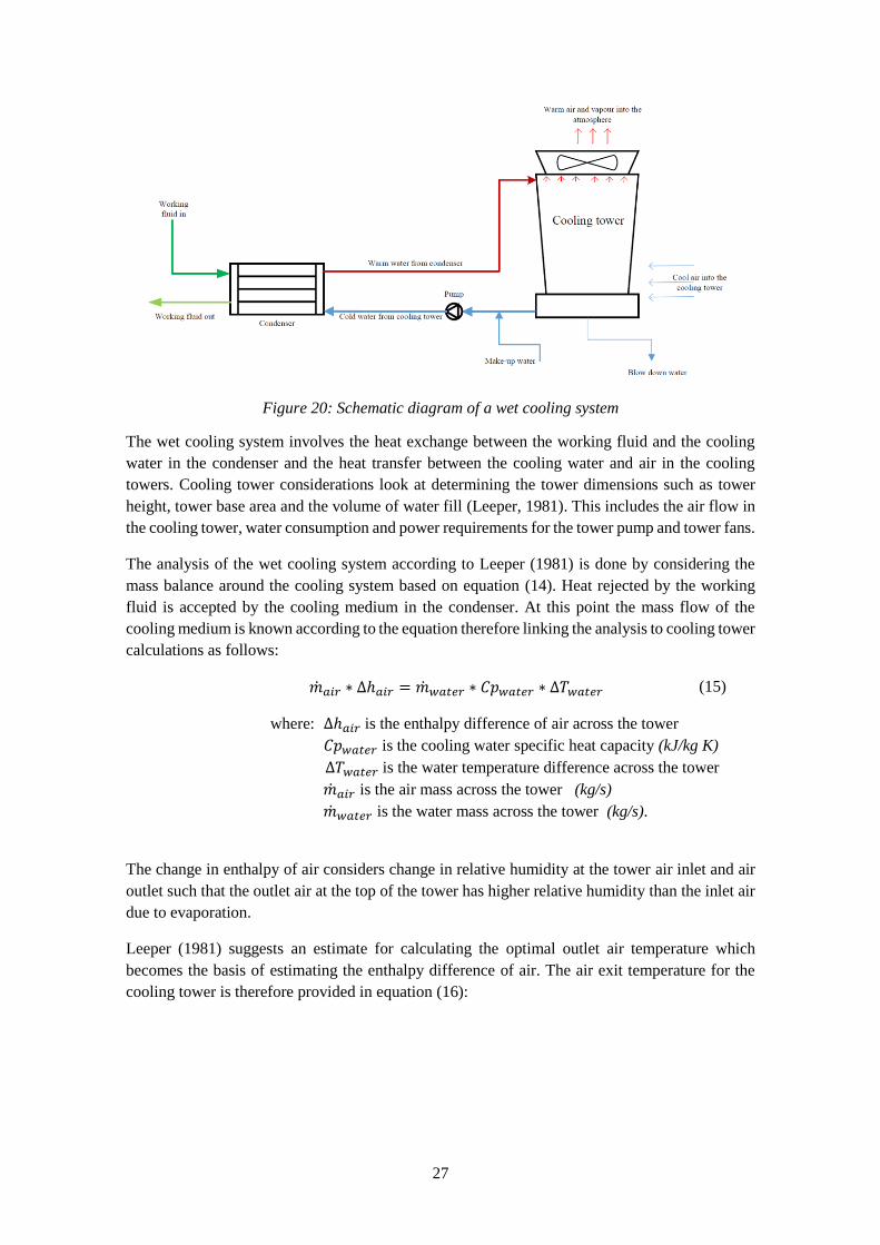
27
Figure 20: Schematic diagram of a wet cooling system
The wet cooling system involves the heat exchange between the working fluid and the cooling
water in the condenser and the heat transfer between the cooling water and air in the cooling
towers. Cooling tower considerations look at determining the tower dimensions such as tower
height, tower base area and the volume of water fill (Leeper, 1981). This includes the air flow in
the cooling tower, water consumption and power requirements for the tower pump and tower fans.
The analysis of the wet cooling system according to Leeper (1981) is done by considering the
mass balance around the cooling system based on equation (14). Heat rejected by the working
fluid is accepted by the cooling medium in the condenser. At this point the mass flow of the
cooling medium is known according to the equation therefore linking the analysis to cooling tower
calculations as follows:
�̇�𝑎𝑖𝑟 ∗ ∆ℎ𝑎𝑖𝑟 = �̇�𝑤𝑎𝑡𝑒𝑟 ∗ 𝐶𝑝𝑤𝑎𝑡𝑒𝑟 ∗ ∆𝑇𝑤𝑎𝑡𝑒𝑟 (15)
where: ∆ℎ𝑎𝑖𝑟 is the enthalpy difference of air across the tower
𝐶𝑝𝑤𝑎𝑡𝑒𝑟 is the cooling water specific heat capacity (kJ/kg K)
∆𝑇𝑤𝑎𝑡𝑒𝑟 is the water temperature difference across the tower
�̇�𝑎𝑖𝑟 is the air mass across the tower (kg/s)
�̇�𝑤𝑎𝑡𝑒𝑟 is the water mass across the tower (kg/s).
The change in enthalpy of air considers change in relative humidity at the tower air inlet and air
outlet such that the outlet air at the top of the tower has higher relative humidity than the inlet air
due to evaporation.
Leeper (1981) suggests an estimate for calculating the optimal outlet air temperature which
becomes the basis of estimating the enthalpy difference of air. The air exit temperature for the
cooling tower is therefore provided in equation (16):
28
𝑡𝑎𝑖𝑟,𝑜𝑢𝑡 =
[𝑇𝑤𝑎𝑡𝑒𝑟,𝑖𝑛 + 𝑇𝑤𝑎𝑡𝑒𝑟,𝑜𝑢𝑡]
2
(16)
where: 𝑡𝑎𝑖𝑟,𝑜𝑢𝑡 is the tower air outlet temperature (°C)
𝑇𝑤𝑎𝑡𝑒𝑟,𝑖𝑛 is the entry temperature of cooling water (°C)
𝑇𝑤𝑎𝑡𝑒𝑟,𝑖𝑛 is the exit temperature of cooling water (°C)
However, given a temperature range as to how far the water can be cooled or how much the air
can be warmed up, the temperature for air at the exit of the tower becomes:
𝑡𝑎𝑖𝑟,𝑜𝑢𝑡 = 𝑡𝑎𝑖𝑟,𝑖𝑛 + 𝑡𝑟𝑎𝑛𝑔𝑒 (°C) (17)
With equations (15) and (17), further parameters for the cooling tower such as the tower height
and base area, may be determined. For pump calculations, Leeper (1981) suggest that the head
for the cooling tower pump HCoolingT as equation (18).
𝐻𝐶𝑜𝑜𝑙𝑖𝑛𝑔,𝑇 = 𝑍𝑑𝑜𝑡 + 10 (18)
where: 𝐻𝐶𝑜𝑜𝑙𝑖𝑛𝑔,𝑇 is the head of the cooling tower
𝑍𝑑𝑜𝑡 is the tower height (m).
The cooling tower pump calculation is therefore given in equation (19)
𝑃𝑐𝑤 = 0.0981 ∗ 𝐻𝐶𝑜𝑜𝑙𝑖𝑛𝑔,𝑇 ∗ 𝑆𝐺𝑤𝑎𝑡𝑒𝑟 (19)
where: 𝑃𝑐𝑤 is the pump power for the cooling tower
𝑆𝐺𝑤𝑎𝑡𝑒𝑟 is the specific gravity for water
The wet cooling system is deemed not to be as efficient as the surface water system, but is more
efficient than the dry cooling system which is discussed below. The chemistry of the water for
cooling must be studied and the water treated to avoid growth of algae or fungi in the cooling
tower (Verkis Consulting Engineers, 2014).
4.2.3. Dry cooling system
The dry cooling system uses air to condense the vapour coming from the turbine. The condenser
is built as a cooling tower with fans that draw air across the condensers. To make the air cooling
effective, the condensing area is spread as wide as possible thereby requiring large area for heat
exchange surface. As a result, the cooling system calls for more use of fans that at times lead to
double as much the power requirement for the fans as compared to wet cooling system
(Mendrinos, et al., 2006). The demand of more fan power increases the parasitic load for the
power plant. Since the system depends on the ambient air, the system is sensitive and subjected
to prevailing ambient temperature variations, both seasonal and hourly variations thereby
affecting the system’s efficiency. A schematic diagram of the dry cooling system is shown in
Figure 21 below.
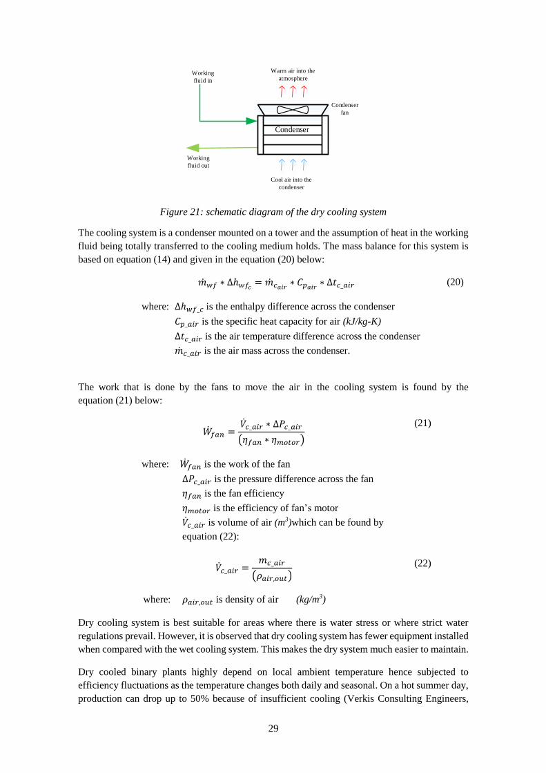
29
Figure 21: schematic diagram of the dry cooling system
The cooling system is a condenser mounted on a tower and the assumption of heat in the working
fluid being totally transferred to the cooling medium holds. The mass balance for this system is
based on equation (14) and given in the equation (20) below:
�̇�𝑤𝑓 ∗ ∆ℎ𝑤𝑓𝑐= �̇�𝑐𝑎𝑖𝑟
∗ 𝐶𝑝𝑎𝑖𝑟∗ ∆𝑡𝑐_𝑎𝑖𝑟 (20)
where: ∆ℎ𝑤𝑓_𝑐 is the enthalpy difference across the condenser
𝐶𝑝_𝑎𝑖𝑟 is the specific heat capacity for air (kJ/kg-K)
∆𝑡𝑐_𝑎𝑖𝑟 is the air temperature difference across the condenser
�̇�𝑐_𝑎𝑖𝑟 is the air mass across the condenser.
The work that is done by the fans to move the air in the cooling system is found by the
equation (21) below:
�̇�𝑓𝑎𝑛 =
�̇�𝑐_𝑎𝑖𝑟 ∗ ∆𝑃𝑐_𝑎𝑖𝑟
(𝜂𝑓𝑎𝑛 ∗ 𝜂𝑚𝑜𝑡𝑜𝑟)
(21)
where: �̇�𝑓𝑎𝑛 is the work of the fan
∆𝑃𝑐_𝑎𝑖𝑟 is the pressure difference across the fan
𝜂𝑓𝑎𝑛 is the fan efficiency
𝜂𝑚𝑜𝑡𝑜𝑟 is the efficiency of fan’s motor
�̇�𝑐_𝑎𝑖𝑟 is volume of air (m3)which can be found by
equation (22):
�̇�𝑐_𝑎𝑖𝑟 =𝑚𝑐_𝑎𝑖𝑟
(𝜌𝑎𝑖𝑟,𝑜𝑢𝑡)
(22)
where: 𝜌𝑎𝑖𝑟,𝑜𝑢𝑡 is density of air (kg/m3)
Dry cooling system is best suitable for areas where there is water stress or where strict water
regulations prevail. However, it is observed that dry cooling system has fewer equipment installed
when compared with the wet cooling system. This makes the dry system much easier to maintain.
Dry cooled binary plants highly depend on local ambient temperature hence subjected to
efficiency fluctuations as the temperature changes both daily and seasonal. On a hot summer day,
production can drop up to 50% because of insufficient cooling (Verkis Consulting Engineers,
Working
fluid out
Condenser
Cool air into the
condenser
Warm air into the
atmosphereWorking
fluid in
Condenser
fan

30
2014). When this type of cooling system is preferred, the fluctuations in ambient temperature
need to be considered.
Malawi is not a water stressed country and the environmental act currently in force only requires
any energy undertaking to conduct a proper environmental impact assessment (EIA) as well as
putting up a robust environmental management plan for the impacts of the undertaking on the
environment. Chiweta being close to water bodies, 1.5 km from Lake Malawi and 500 m from
North Rumphi River, may not pause very significant environmental impact by using water within
its reach. With the abundance of water coupled with favourable climatic conditions of good
average temperature all year round, Chiweta may implement an air cooled or water cooled system.
Both systems will be subjected to analysis in the next sections.
4.3. Consideration of scaling potential
When the geothermal water is in the reservoir, it interacts with the host rock and in the process
dissolves some constituents from the rocks until they reach a chemical equilibrium at reservoir
conditions. This depends on a number of factors such as the geology of the resource, temperature,
pressure as well as the source of the water. Different fields will therefore have geothermal fluid
with different chemical compositions depending on these factors. As the geothermal water is
being transferred from the reservoir for various utilization undertakings, the physical and
chemical conditions of the water changes and some of the dissolved constituents may no longer
remain soluble in the water thereby forming depositions along the way. Some of the minerals
exhibit higher solubility in water where the temperature of water increases and when the water
temperature starts to decrease, the dissolved minerals become less soluble thereby precipitating
from the solution (DiPippo, 2012). Other minerals will precipitate where the fluid is being flashed
and a portion of the fluid turns into steam (Nugroho, 2011). Such deposition and precipitation of
minerals occurs on the surface of power plant equipment or in the wells and is experienced in
many geothermal power plants. Problems such as equipment damage and failure, brine leaks and
spills, well and line plugging, reduced brine flow and power production losses are some of the
experiences associated with scaling. Dealing with scaling in production wells or power plant
equipment proves to be normally expensive since they introduce cleaning expenses over and
above reduced production. As such prevention is serving as a better option (Brown, 2013). The
major scaling threats in geothermal power plants are calcite and silica scaling.
Calcite scaling occurs near the flash point in the production wells due to a decrease in calcite
solubility as some fluid turns to vapour. Calcium solubility varies with the pressure of carbon
dioxide (CO2) and temperature of the fluid (Yanagisawa, 2015). Prevention of calcite scaling in
wells is mostly by using various chemical inhibitors such as sodium polyacrylate. A capillary tube
is inserted into a production well to the depth of flashing point where the chemical inhibitor is
directly injected for scaling prevention (Yanagisawa, 2015). With calcite scaling, there is little
that can be done at design stage for its prevention. One of the ways of prevention is by preventing
flashing in the production well by keeping well head pressures sufficiently high thereby
maintaining the fluid in liquid phase.
Silica exists in different forms such as quartz, tridymite, cristobalite, amorphous silica and many
others (Brown, 2013). Of all these forms, amorphous silica and quartz are much associated with
geothermal scaling problems (DiPippo, 1985). As such, silica scaling is analysed using the
amorphous silica and quartz concentration in the fluid. When the geothermal water is in the
reservoir, the solubility of silica is controlled by quartz but as the water is cooling down, silica
solubility is controlled by amorphous silica (DiPippo, 2012). Amorphous silica is more soluble
31
than quartz and this provides a window of opportunity to utilize the geothermal fluid between the
quartz solubility curve and the amorphous silica solubility curve without experiencing silica
scaling (Brown, 2013) as the fluid tends to precipitate the silica through flashing and lowering
temperature. Beyond the amorphous silica solubility curve, scaling is inevitable.
Since the chemistry of Chiweta field which is under study is not fully known at the moment, a
general considerations for scaling potential is therefore made to account for a reasonable
reinjection temperature that considers potential of scaling. It is anticipated that the fluid in the
Chiweta field may have a higher value of pH (GDC - Kenya, 2010) and therefore there may be
more precipitation of some minerals since mineral precipitation is also affected by the pH value
of the fluid (DiPippo, 1985).
To achieve maximum utilization of a geothermal resource, the geothermal fluid must be cooled
to the lowest temperatures possible. However, as the cooling is taking place, the geothermal fluid
becomes supersaturated with minerals such as silica and precipitation begins. As a result, a
temperature that allows geothermal exploitation without the possibility of silica scaling needs to
be assessed. This temperature, the silica saturation temperature (SST), is the temperature of the
geothermal fluid at the exit of the heat exchanger before the fluid reaches saturation with respect
to the amorphous silica (Brown, 2013). When in the reservoir, silica concentration is controlled
by quartz while in the surface equipment the concentration is mostly controlled by amorphous
silica.
In the absence of data, analysis of amorphous silica solubility is done using the equation (23)
below with respect to temperature. This gives the SST for a given resource temperature. The
equation is true for temperature range of 0° – 250°C (Utami, et al., 2014).
log 𝐶 = (−
731
𝑇+ 4.52)
(23)
where: C is the amorphous silica concentration (mg/L)
T is the absolute temperature (°K).
According to DiPippo (2012), the quartz solubility estimate with respect to temperature is given
by equation (24) below:
Q(𝑡) = 41.598 + 0.23932𝑡 – 0.011172𝑡2 + 1.1713 ∗ 10−4𝑡3 – 1.9708 ∗ 10−7𝑡4 (24)
where: Q is the silica concentration (mg/kg).
t is the reservoir temperature (°C).
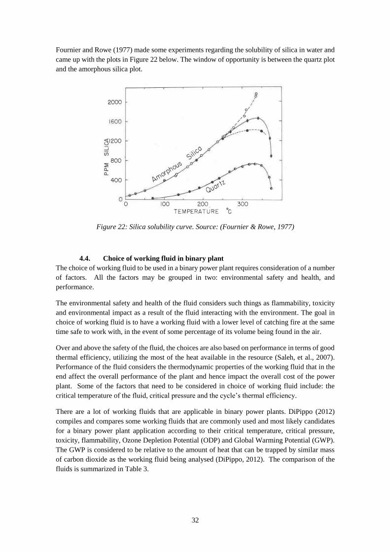
32
Fournier and Rowe (1977) made some experiments regarding the solubility of silica in water and
came up with the plots in Figure 22 below. The window of opportunity is between the quartz plot
and the amorphous silica plot.
Figure 22: Silica solubility curve. Source: (Fournier & Rowe, 1977)
4.4. Choice of working fluid in binary plant
The choice of working fluid to be used in a binary power plant requires consideration of a number
of factors. All the factors may be grouped in two: environmental safety and health, and
performance.
The environmental safety and health of the fluid considers such things as flammability, toxicity
and environmental impact as a result of the fluid interacting with the environment. The goal in
choice of working fluid is to have a working fluid with a lower level of catching fire at the same
time safe to work with, in the event of some percentage of its volume being found in the air.
Over and above the safety of the fluid, the choices are also based on performance in terms of good
thermal efficiency, utilizing the most of the heat available in the resource (Saleh, et al., 2007).
Performance of the fluid considers the thermodynamic properties of the working fluid that in the
end affect the overall performance of the plant and hence impact the overall cost of the power
plant. Some of the factors that need to be considered in choice of working fluid include: the
critical temperature of the fluid, critical pressure and the cycle’s thermal efficiency.
There are a lot of working fluids that are applicable in binary power plants. DiPippo (2012)
compiles and compares some working fluids that are commonly used and most likely candidates
for a binary power plant application according to their critical temperature, critical pressure,
toxicity, flammability, Ozone Depletion Potential (ODP) and Global Warming Potential (GWP).
The GWP is considered to be relative to the amount of heat that can be trapped by similar mass
of carbon dioxide as the working fluid being analysed (DiPippo, 2012). The comparison of the
fluids is summarized in Table 3.

33
Table 3: Properties of binary plant working fluids. Source: modified from DiPippo, (2012)
From Table 3, the fluids exhibit lower values of critical temperature and pressure as compared to
water. This helps to reduce thermodynamic losses in the heat exchangers hence making the fluids
ideal for use in binary power plant application (DiPippo, 2012). Almost all the fluids as presented
by DiPippo have a low toxicity as well as low ODP and global warming potential with reference
to their release of carbon dioxide into the atmosphere. Despite not being toxic and flammable,
R-12 and R-114 exhibit high ODP and GWP thereby pausing an environmental hazard. R-12 and
R-114 have since been banned from use in binary plant application (DiPippo, 2012).
Further to the parameters compared by DiPippo (2012), the shape of the saturation vapour curve
in the T-s diagram is also considered. Working fluids are divided into three types according to
their saturation vapour curves. Bao and Zhao (2013) gives the three types of working fluids as:
the wet fluids, isentropic fluids and dry fluids. The dry fluids exhibit a positive slope of a
saturation curve in a T-s diagram while the wet fluids have a negative slope just like water, and
ammonia is an example of wet fluids (Bao & Zhao, 2013). The isentropic fluids exhibit a nearly
infinitely large slope which is almost vertical. Examples of isentropic fluids include flourinal 85
and R-11. The isentropic fluids remain in a vapour saturated state as they expands through the
turbine since the expansion occurs along the vertical line of the T-s diagram. This results in the
fluid not condensing at the turbine outlet thereby the turbine not experiencing liquid droplets from
the working fluid.
Wet fluids normally leave some level of saturated liquid at the turbine outlet due to their negative
saturation vapour curve which may damage the turbine blades. To sustain operations with wet
fluids in binary power plant, the fluid is normally superheated at the turbine inlet and the dryness
fraction of fluid is kept at above 85% (Bao & Zhao, 2013) below which, damage to the turbine
blades becomes severe. The isentropic and dry fluids generally do not need superheating and
minimum dryness fraction since they are already in the vapour saturated phase at the turbine exit
(DiPippo, 2012). This is the reason why in most binary applications, the dry fluids and the
isentropic fluids are commonly used as they do not form condensate as they pass through the
turbine. The dry fluids, sometimes known as retrograde fluids, that are commonly used in power
plants are normal butane, isobutene, normal pentane and isopentane. Figure 23 depicts the T-s
diagrams of different fluid types as discussed.
Fluid Formula Critical Temp
(°C)
Critical Pressure
(bar)
Toxicity Flammability ODP GWP
R-12 CCl2F2 - - Non-toxic Non-flammable 1 4500
R-114 C2Cl2F4 - - Non-toxic Non-flammable 0.7 5850
Propane C3H8 96.95 42.36 low very high 0 3
i-Butane i-C4H10 135.92 36.85 low very high 0 3
n-Butane C4H10 150.8 37.18 low very high 0 3
i-Pentane i-C5H12 187.8 34.09 low very high 0 3
n-Pentane C5H12 193.9 32.4 low very high 0 3
Ammonia NH3 133.65 116.27 low lower 0 0
Water H2O 374.14 220.89 Non-toxic Non-flammable 0 -
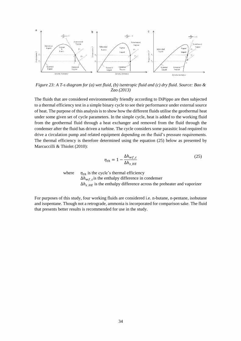
34
Figure 23: A T-s diagram for (a) wet fluid, (b) isentropic fluid and (c) dry fluid. Source: Bao &
Zao (2013)
The fluids that are considered environmentally friendly according to DiPippo are then subjected
to a thermal efficiency test in a simple binary cycle to see their performance under external source
of heat. The purpose of this analysis is to show how the different fluids utilise the geothermal heat
under some given set of cycle parameters. In the simple cycle, heat is added to the working fluid
from the geothermal fluid through a heat exchanger and removed from the fluid through the
condenser after the fluid has driven a turbine. The cycle considers some parasitic load required to
drive a circulation pump and related equipment depending on the fluid’s pressure requirements.
The thermal efficiency is therefore determined using the equation (25) below as presented by
Marcuccilli & Thiolet (2010):
𝜂𝑡ℎ = 1 −
∆ℎ𝑤𝑓_𝑐
∆ℎ𝑠_𝐻𝐸
(25)
where 𝜂𝑡ℎ is the cycle’s thermal efficiency
∆ℎ𝑤𝑓_𝑐is the enthalpy difference in condenser
∆ℎ𝑠_𝐻𝐸 is the enthalpy difference across the preheater and vaporizer
For purposes of this study, four working fluids are considered i.e. n-butane, n-pentane, isobutane
and isopentane. Though not a retrograde, ammonia is incorporated for comparison sake. The fluid
that presents better results is recommended for use in the study.

35
5.0. Modelling of the binary power plant Modelling of the power plant is done using the Engineering Equation Solver (EES) Program. EES
program provides solutions of set algebraic equations, differential equations and do various
optimizations and analyses while generating plots to the analyses. EES program has a library of
mathematical and thermophysical properties of vast number of fluids that are associated with
geothermal plant cycles. These built-in functions of steam tables facilitate thermodynamic
modelling of geothermal power plants. Modelling of the power plant assumes that the cycle
reaches a steady state and that pressure drops in pipes and heat exchangers as well as heat losses
to the environment in the turbine and all the heat exchangers in the cycle are negligible unless
stated otherwise in the process wherever necessary.
5.1. Boundary conditions
Boundary conditions provide input parameters to the model based on data at hand. Where data is
not available, some reasonable assumptions based on literature review are made as reasonable as
possible. The boundary conditions for this work include geothermal fluid mass flow, working
fluid for the cycle, equipment efficiency, pressures and temperatures and are discussed further in
the next sections below.
5.1.1. Fluid gathering system
Even though the GDC-Kenya report (2010) proposes a subsurface of 249°C in Chiweta, this study
considers a lower temperature to be in tandem with the generally experienced geothermal gradient
of the western branch of the EARS (Kraml, et al., 2010). The proposed subsurface temperature
indicates that Chiweta has a good geothermal resource, however being within the western branch,
this study proposes a temperature of 180°C and this is used in the modelling. It is generally
expected that at such temperatures, the production well would be artesian and that fluid may start
boiling at some point and producing steam along the way. This study bears in mind that such
expectations are site specific and that there is need to have field characteristics to incorporate such
behaviour in power plant modelling. With only temperature at hand and without necessary field
characteristics, it is better to assume that production wells are non-artesian as such pumping is
required. In this aspect, the pumping assures of geothermal fluid that is kept in liquid phase and
thereby acting as a preventive measure in calcite scaling. The pumping parasitic load is accounted
for in the total parasitic load of a given power plant. Further work is recommended to validate the
reservoir temperature and characteristics of the field.
Fluid gathering system requires field characteristics such as borehole pressure and well discharge
from production wells. Chiweta has little information regarding the field characteristics and
therefore fluid gathering system may be speculated at this time. Since the model considers calcite
prevention in a way of maintaining the geothermal fluid in liquid phase, the geo-fluid pressure is
kept at slightly above the saturation pressure of the reservoir temperature. The saturation reservoir
pressure at 180°C temperature is 10.03 bars. Considering that the fluid may lose some pressure
along its path through the system to the reinjection well, consideration is made to keep the fluid
from boiling even as it loses pressure in the system. As such 1 bar is added to the saturation
pressure of the geo-fluid, hence the considered pressure for geo-fluid in this work is 11.03 bars.
Mass flow of a geothermal field is more dependent on the permeability of the reservoir. Generally,
wells drilled in medium to low temperature geothermal field may have the capacity of delivering
geothermal liquid of 20 – 60 kg/s (Mannvit - Geoelec, 2012). It is therefore likely that a
geothermal well in low to medium temperature may deliver 40 kg/s which is also in agreement
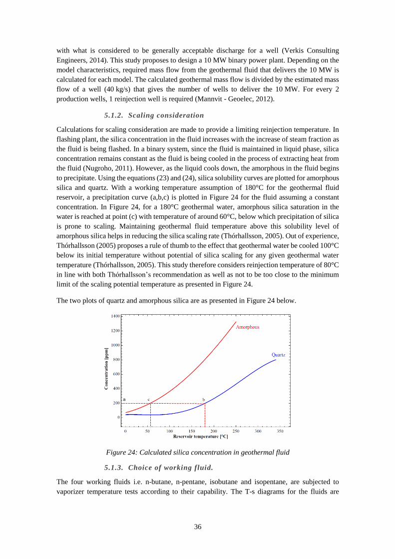
36
with what is considered to be generally acceptable discharge for a well (Verkis Consulting
Engineers, 2014). This study proposes to design a 10 MW binary power plant. Depending on the
model characteristics, required mass flow from the geothermal fluid that delivers the 10 MW is
calculated for each model. The calculated geothermal mass flow is divided by the estimated mass
flow of a well (40 kg/s) that gives the number of wells to deliver the 10 MW. For every 2
production wells, 1 reinjection well is required (Mannvit - Geoelec, 2012).
5.1.2. Scaling consideration
Calculations for scaling consideration are made to provide a limiting reinjection temperature. In
flashing plant, the silica concentration in the fluid increases with the increase of steam fraction as
the fluid is being flashed. In a binary system, since the fluid is maintained in liquid phase, silica
concentration remains constant as the fluid is being cooled in the process of extracting heat from
the fluid (Nugroho, 2011). However, as the liquid cools down, the amorphous in the fluid begins
to precipitate. Using the equations (23) and (24), silica solubility curves are plotted for amorphous
silica and quartz. With a working temperature assumption of 180°C for the geothermal fluid
reservoir, a precipitation curve (a,b,c) is plotted in Figure 24 for the fluid assuming a constant
concentration. In Figure 24, for a 180°C geothermal water, amorphous silica saturation in the
water is reached at point (c) with temperature of around 60°C, below which precipitation of silica
is prone to scaling. Maintaining geothermal fluid temperature above this solubility level of
amorphous silica helps in reducing the silica scaling rate (Thórhallsson, 2005). Out of experience,
Thórhallsson (2005) proposes a rule of thumb to the effect that geothermal water be cooled 100°C
below its initial temperature without potential of silica scaling for any given geothermal water
temperature (Thórhallsson, 2005). This study therefore considers reinjection temperature of 80°C
in line with both Thórhallsson’s recommendation as well as not to be too close to the minimum
limit of the scaling potential temperature as presented in Figure 24.
The two plots of quartz and amorphous silica are as presented in Figure 24 below.
Figure 24: Calculated silica concentration in geothermal fluid
5.1.3. Choice of working fluid.
The four working fluids i.e. n-butane, n-pentane, isobutane and isopentane, are subjected to
vaporizer temperature tests according to their capability. The T-s diagrams for the fluids are
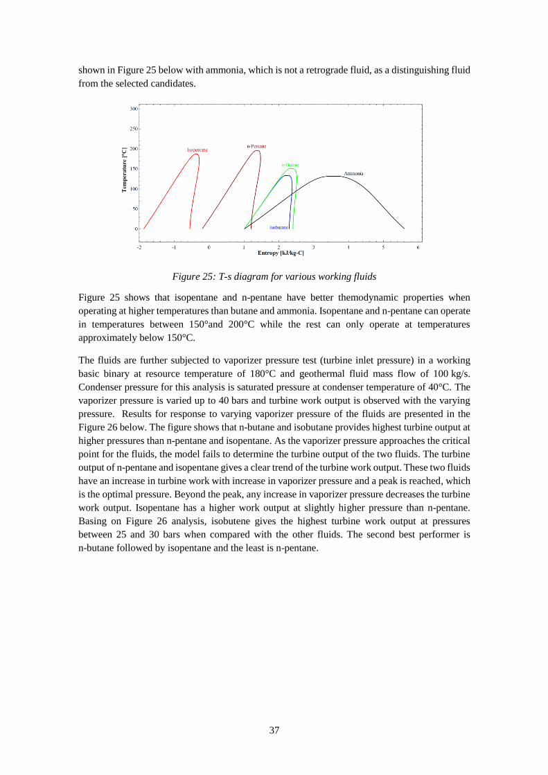
37
shown in Figure 25 below with ammonia, which is not a retrograde fluid, as a distinguishing fluid
from the selected candidates.
Figure 25: T-s diagram for various working fluids
Figure 25 shows that isopentane and n-pentane have better themodynamic properties when
operating at higher temperatures than butane and ammonia. Isopentane and n-pentane can operate
in temperatures between 150°and 200°C while the rest can only operate at temperatures
approximately below 150°C.
The fluids are further subjected to vaporizer pressure test (turbine inlet pressure) in a working
basic binary at resource temperature of 180°C and geothermal fluid mass flow of 100 kg/s.
Condenser pressure for this analysis is saturated pressure at condenser temperature of 40°C. The
vaporizer pressure is varied up to 40 bars and turbine work output is observed with the varying
pressure. Results for response to varying vaporizer pressure of the fluids are presented in the
Figure 26 below. The figure shows that n-butane and isobutane provides highest turbine output at
higher pressures than n-pentane and isopentane. As the vaporizer pressure approaches the critical
point for the fluids, the model fails to determine the turbine output of the two fluids. The turbine
output of n-pentane and isopentane gives a clear trend of the turbine work output. These two fluids
have an increase in turbine work with increase in vaporizer pressure and a peak is reached, which
is the optimal pressure. Beyond the peak, any increase in vaporizer pressure decreases the turbine
work output. Isopentane has a higher work output at slightly higher pressure than n-pentane.
Basing on Figure 26 analysis, isobutene gives the highest turbine work output at pressures
between 25 and 30 bars when compared with the other fluids. The second best performer is
n-butane followed by isopentane and the least is n-pentane.
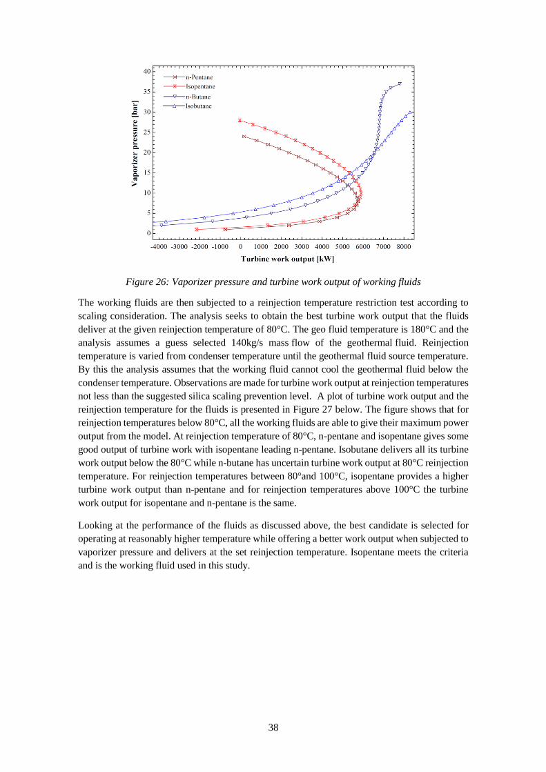
38
Figure 26: Vaporizer pressure and turbine work output of working fluids
The working fluids are then subjected to a reinjection temperature restriction test according to
scaling consideration. The analysis seeks to obtain the best turbine work output that the fluids
deliver at the given reinjection temperature of 80°C. The geo fluid temperature is 180°C and the
analysis assumes a guess selected 140kg/s mass flow of the geothermal fluid. Reinjection
temperature is varied from condenser temperature until the geothermal fluid source temperature.
By this the analysis assumes that the working fluid cannot cool the geothermal fluid below the
condenser temperature. Observations are made for turbine work output at reinjection temperatures
not less than the suggested silica scaling prevention level. A plot of turbine work output and the
reinjection temperature for the fluids is presented in Figure 27 below. The figure shows that for
reinjection temperatures below 80°C, all the working fluids are able to give their maximum power
output from the model. At reinjection temperature of 80°C, n-pentane and isopentane gives some
good output of turbine work with isopentane leading n-pentane. Isobutane delivers all its turbine
work output below the 80°C while n-butane has uncertain turbine work output at 80°C reinjection
temperature. For reinjection temperatures between 80°and 100°C, isopentane provides a higher
turbine work output than n-pentane and for reinjection temperatures above 100°C the turbine
work output for isopentane and n-pentane is the same.
Looking at the performance of the fluids as discussed above, the best candidate is selected for
operating at reasonably higher temperature while offering a better work output when subjected to
vaporizer pressure and delivers at the set reinjection temperature. Isopentane meets the criteria
and is the working fluid used in this study.
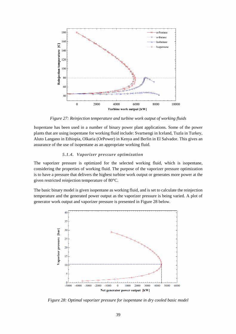
39
Figure 27: Reinjection temperature and turbine work output of working fluids
Isopentane has been used in a number of binary power plant applications. Some of the power
plants that are using isopentane for working fluid include: Svartsengi in Iceland, Tuzla in Turkey,
Aluto Langano in Ethiopia, Olkaria (OrPower) in Kenya and Berlin in El Salvador. This gives an
assurance of the use of isopentane as an appropriate working fluid.
5.1.4. Vaporizer pressure optimization
The vaporizer pressure is optimized for the selected working fluid, which is isopentane,
considering the properties of working fluid. The purpose of the vaporizer pressure optimization
is to have a pressure that delivers the highest turbine work output or generates more power at the
given restricted reinjection temperature of 80°C.
The basic binary model is given isopentane as working fluid, and is set to calculate the reinjection
temperature and the generated power output as the vaporizer pressure is being varied. A plot of
generator work output and vaporizer pressure is presented in Figure 28 below.
Figure 28: Optimal vaporizer pressure for isopentane in dry cooled basic model
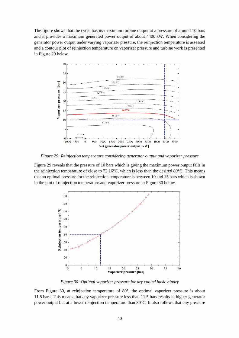
40
The figure shows that the cycle has its maximum turbine output at a pressure of around 10 bars
and it provides a maximum generated power output of about 4400 kW. When considering the
generator power output under varying vaporizer pressure, the reinjection temperature is assessed
and a contour plot of reinjection temperature on vaporizer pressure and turbine work is presented
in Figure 29 below.
Figure 29: Reinjection temperature considering generator output and vaporizer pressure
Figure 29 reveals that the pressure of 10 bars which is giving the maximum power output falls in
the reinjection temperature of close to 72.16°C, which is less than the desired 80°C. This means
that an optimal pressure for the reinjection temperature is between 10 and 15 bars which is shown
in the plot of reinjection temperature and vaporizer pressure in Figure 30 below.
Figure 30: Optimal vaporizer pressure for dry cooled basic binary
From Figure 30, at reinjection temperature of 80°, the optimal vaporizer pressure is about
11.5 bars. This means that any vaporizer pressure less than 11.5 bars results in higher generator
power output but at a lower reinjection temperature than 80°C. It also follows that any pressure

41
above 11.5 bars results in lower generator power output at a higher reinjection temperature than
80°C. Based on this understanding, this study therefore uses 12 bars as optimal vaporizer
pressure, for the basic binary model which assures of reinjection temperature of not less than
80°C. The same procedure is performed for the wet cooled basic model, dry and wet cooled
recuperative models (appendices 1 to 3) and the optimal vaporizer pressure for all these models
is 11 bars.
5.1.5. Efficiencies of equipment and associated parameters
Typically, the efficiency of turbines are in the range of 81-85% (Dickson & Fanell, 2003) and this
study uses turbine work efficiency of 85% as it looks forward to having the best performing
turbine implemented for such a project. The fan efficiency for the cooling system used in this
work is 70% and the pump efficiency used for all pump requirements is 80% (Frick, et al., 2015).
The motor efficiency for all the motors used in pumps and fans is 95%. The generator efficiency
assumes 95% (Mendrinos, et al., 2006). The overall heat transfer coefficients for heat exchangers
in this study are based on Ahangar (2012) where preheater has 1000 W/m2°C, vaporizer has
1600 W/m2°C, recuperator has 400 W/m2°C and condenser has 800 W/m2°C (Ahangar, 2012).
The pinch temperature used for all the heat exchangers in this work is 5°C (Marcuccilli & Thiolet,
2010). Usually the choice of a pinch temperature is an optimization issue of efficiency and cost
of the heat exchangers. However, the final pinch selection is usually based on the vendor’s
available pinch (Verkis Consulting Engineers, 2014). The air-side pressure drop for both air
cooled condenser and the cooling tower fans (∆PAcc) is 175 Pa (Ashwood & Bharathan, 2011).
The wet cooling system assumes a cooling tower height of 4.645 m (Ura & Saitou, 2000).
The condensing temperature used in this study is calculated as ambient temperature. The
condensing temperature may be optimized by considering the efficiency of the cycle and the cost
of the condenser. However, this work has chosen a fixed condensing temperature since choice by
optimal condenser cost may be subjective and requires a number of guessing and iterations which
may be beyond the scope of this work.
5.1.6. Local ambient conditions
Atmospheric pressure varies with altitude in metres above sea level (masl). The higher you go
from the sea level, the lower the atmospheric pressure. The altitude of Chiweta is 500 masl and
therefore the atmospheric pressure for the area is found by the equation (26) below:
𝑃𝑎𝑖𝑟,𝑎𝑙𝑡 =𝑃𝑎𝑡𝑚,𝑧𝑒𝑟𝑜−𝜌𝑎𝑖𝑟∗𝑔∗𝑎𝑙𝑡𝑖𝑡𝑢𝑑𝑒
100,000 (bars) (26)
where 𝑃𝑎𝑖𝑟,𝑎𝑙𝑡 is the atmospheric pressure at altitude
𝑃𝑎𝑡𝑚,𝑧𝑒𝑟𝑜 is the atmospheric pressure at sea level
𝜌𝑎𝑖𝑟 is the density of air
𝑎𝑙𝑡𝑖𝑡𝑢𝑑𝑒 is the site elevation above sea level
This gives the atmospheric pressure of Chiweta as 0.9495 bars and this is used in this work.
The average ambient temperature used in the model is 24°C (Climate Data, 2015); the relative
humidity is 70% (ClimaTemps.com, 2015)and the Lake Malawi water surface temperature is
23°C (Programme U, 2015). With the given air and water temperatures, a condensing temperature

42
of 40°C is selected for calculating condenser parameters. This is used to find the temperature
range of the condenser and subsequently determining the condenser size.
A summary of the boundary conditions is presented in Table 4 below.
Table 4: Common boundary conditions for the models
Parameter Value Unit
Working fluid Isopentane
Geothermal fluid source pressure 11.03 bar
Atmospheric pressure 0.9495 bar
Vaporizer pressure (basic and recuperative) 12 & 11 bar
Condenser pressure 1.513 bar
Pressure change in fan (∆PAcc) 175 Pa
Geothermal fluid source temperature 180 °C
Condenser temperature 40 °C
Vaporizer-Preheater pinch temperature difference 5 °C
Condenser pinch temperature difference 5 °C
Surface water temperature 23 °C
Ambient temperature for Chiweta 24 °C
Relative humidity for Chiweta 70 %
Fan efficiency 70 %
Feed pump efficiency 80 %
Turbine efficiency 85 %
Generator efficiency 95 %
Motor efficiency (for pump and fan) 95 %
Preheater heat transfer coefficient 1000 W/m2°C
Vaporizer heat transfer coefficient 1600 W/m2°C
Recuperator heat transfer coefficient 400 W/m2°C
Condenser heat transfer coefficient 800 W/m2°C
5.2. Modelling of scenarios and results
The modelling is based on four scenarios which are: basic binary plant with dry cooling system,
basic binary plant with wet cooling system, regenerative binary with dry cooling system and
regenerative plant with wet cooling system. The boundary conditions discussed in the previous
section are applied to the binary system in an EES model.
The performance of the models are as follows:
5.2.1. Basic binary with dry and wet cooling system
The vaporizer pressure of 12 bars is used in the dry cooled basic binary models, 11 bars for the
wet cooled model and the models are set to calculate the required geothermal fluid mass flow for
producing a net generator power output of 10 MW. A plot of required geothermal fluid mass flow
and generator power output for the dry cooled basic model is presented in Figure 31 below. The
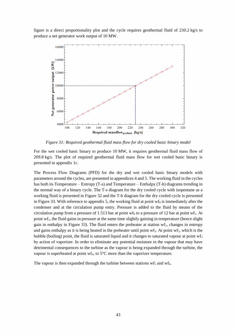
43
figure is a direct proportionality plot and the cycle requires geothermal fluid of 230.2 kg/s to
produce a net generator work output of 10 MW.
Figure 31: Required geothermal fluid mass flow for dry cooled basic binary model
For the wet cooled basic binary to produce 10 MW, it requires geothermal fluid mass flow of
209.8 kg/s. The plot of required geothermal fluid mass flow for wet cooled basic binary is
presented in appendix 1c.
The Process Flow Diagrams (PFD) for the dry and wet cooled basic binary models with
parameters around the cycles, are presented in appendices 4 and 5. The working fluid in the cycles
has both its Temperature – Entropy (T-s) and Temperature – Enthalpy (T-h) diagrams trending in
the normal way of a binary cycle. The T-s diagram for the dry cooled cycle with isopentane as a
working fluid is presented in Figure 32 and the T-h diagram for the dry cooled cycle is presented
in Figure 33. With reference to appendix 5, the working fluid at point wf8 is immediately after the
condenser and at the circulation pump entry. Pressure is added to the fluid by means of the
circulation pump from a pressure of 1.513 bar at point wf8 to a pressure of 12 bar at point wf1. At
point wf1, the fluid gains in pressure at the same time slightly gaining in temperature (hence slight
gain in enthalpy in Figure 33). The fluid enters the preheater at station wf1, changes in entropy
and gains enthalpy as it is being heated in the preheater until point wf2. At point wf2, which is the
bubble (boiling) point, the fluid is saturated liquid and it changes to saturated vapour at point wf3
by action of vaporizer. In order to eliminate any potential moisture in the vapour that may have
detrimental consequences to the turbine as the vapour is being expanded through the turbine, the
vapour is superheated at point wf4, to 5°C more than the vaporizer temperature.
The vapour is then expanded through the turbine between stations wf5 and wf6.
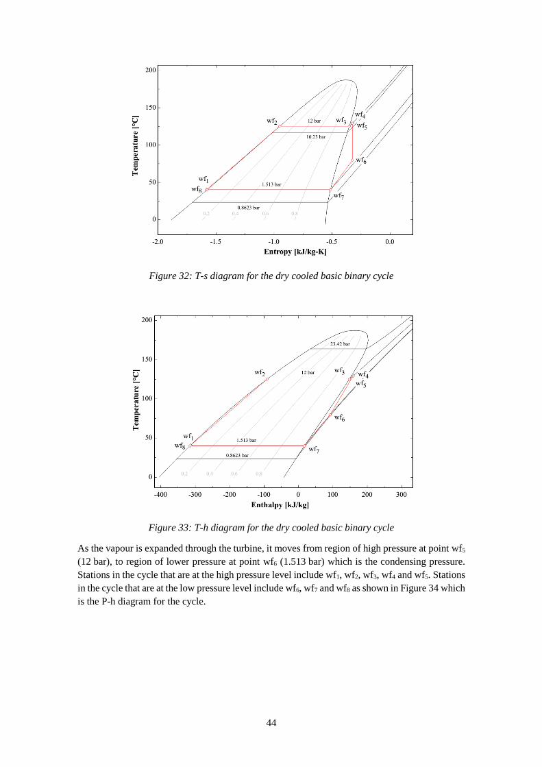
44
Figure 32: T-s diagram for the dry cooled basic binary cycle
Figure 33: T-h diagram for the dry cooled basic binary cycle
As the vapour is expanded through the turbine, it moves from region of high pressure at point wf5
(12 bar), to region of lower pressure at point wf6 (1.513 bar) which is the condensing pressure.
Stations in the cycle that are at the high pressure level include wf1, wf2, wf3, wf4 and wf5. Stations
in the cycle that are at the low pressure level include wf6, wf7 and wf8 as shown in Figure 34 which
is the P-h diagram for the cycle.
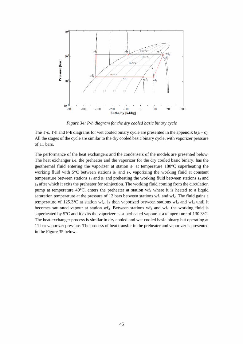
45
Figure 34: P-h diagram for the dry cooled basic binary cycle
The T-s, T-h and P-h diagrams for wet cooled binary cycle are presented in the appendix 6(a – c).
All the stages of the cycle are similar to the dry cooled basic binary cycle, with vaporizer pressure
of 11 bars.
The performance of the heat exchangers and the condensers of the models are presented below.
The heat exchanger i.e. the preheater and the vaporizer for the dry cooled basic binary, has the
geothermal fluid entering the vaporizer at station s1 at temperature 180°C superheating the
working fluid with 5°C between stations s1 and s2, vaporizing the working fluid at constant
temperature between stations s2 and s3 and preheating the working fluid between stations s3 and
s4 after which it exits the preheater for reinjection. The working fluid coming from the circulation
pump at temperature 40°C, enters the preheater at station wf1 where it is heated to a liquid
saturation temperature at the pressure of 12 bars between stations wf1 and wf2. The fluid gains a
temperature of 125.3°C at station wf2, is then vaporized between stations wf2 and wf3 until it
becomes saturated vapour at station wf3. Between stations wf3 and wf4, the working fluid is
superheated by 5°C and it exits the vaporizer as superheated vapour at a temperature of 130.3°C.
The heat exchanger process is similar in dry cooled and wet cooled basic binary but operating at
11 bar vaporizer pressure. The process of heat transfer in the preheater and vaporizer is presented
in the Figure 35 below.
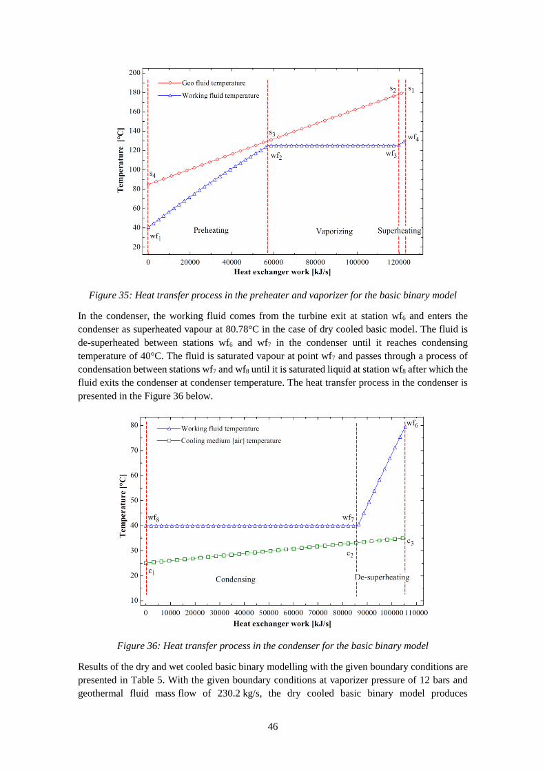
46
Figure 35: Heat transfer process in the preheater and vaporizer for the basic binary model
In the condenser, the working fluid comes from the turbine exit at station wf6 and enters the
condenser as superheated vapour at 80.78°C in the case of dry cooled basic model. The fluid is
de-superheated between stations wf6 and wf7 in the condenser until it reaches condensing
temperature of 40°C. The fluid is saturated vapour at point wf7 and passes through a process of
condensation between stations wf7 and wf8 until it is saturated liquid at station wf8 after which the
fluid exits the condenser at condenser temperature. The heat transfer process in the condenser is
presented in the Figure 36 below.
Figure 36: Heat transfer process in the condenser for the basic binary model
Results of the dry and wet cooled basic binary modelling with the given boundary conditions are
presented in Table 5. With the given boundary conditions at vaporizer pressure of 12 bars and
geothermal fluid mass flow of 230.2 kg/s, the dry cooled basic binary model produces
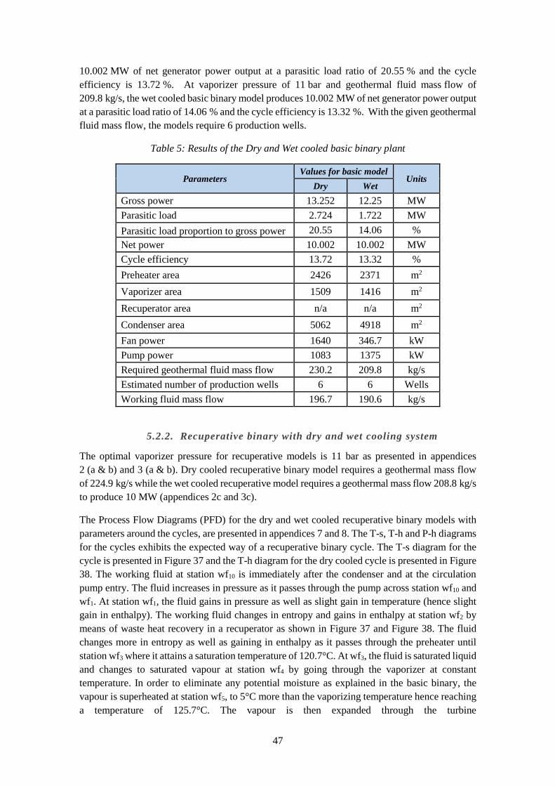
47
10.002 MW of net generator power output at a parasitic load ratio of 20.55 % and the cycle
efficiency is 13.72 %. At vaporizer pressure of 11 bar and geothermal fluid mass flow of
209.8 kg/s, the wet cooled basic binary model produces 10.002 MW of net generator power output
at a parasitic load ratio of 14.06 % and the cycle efficiency is 13.32 %. With the given geothermal
fluid mass flow, the models require 6 production wells.
Table 5: Results of the Dry and Wet cooled basic binary plant
Parameters Values for basic model
Units Dry Wet
Gross power 13.252 12.25 MW
Parasitic load 2.724 1.722 MW
Parasitic load proportion to gross power 20.55 14.06 %
Net power 10.002 10.002 MW
Cycle efficiency 13.72 13.32 %
Preheater area 2426 2371 m2
Vaporizer area 1509 1416 m2
Recuperator area n/a n/a m2
Condenser area 5062 4918 m2
Fan power 1640 346.7 kW
Pump power 1083 1375 kW
Required geothermal fluid mass flow 230.2 209.8 kg/s
Estimated number of production wells 6 6 Wells
Working fluid mass flow 196.7 190.6 kg/s
5.2.2. Recuperative binary with dry and wet cooling system
The optimal vaporizer pressure for recuperative models is 11 bar as presented in appendices
2 (a & b) and 3 (a & b). Dry cooled recuperative binary model requires a geothermal mass flow
of 224.9 kg/s while the wet cooled recuperative model requires a geothermal mass flow 208.8 kg/s
to produce 10 MW (appendices 2c and 3c).
The Process Flow Diagrams (PFD) for the dry and wet cooled recuperative binary models with
parameters around the cycles, are presented in appendices 7 and 8. The T-s, T-h and P-h diagrams
for the cycles exhibits the expected way of a recuperative binary cycle. The T-s diagram for the
cycle is presented in Figure 37 and the T-h diagram for the dry cooled cycle is presented in Figure
38. The working fluid at station wf10 is immediately after the condenser and at the circulation
pump entry. The fluid increases in pressure as it passes through the pump across station wf10 and
wf1. At station wf1, the fluid gains in pressure as well as slight gain in temperature (hence slight
gain in enthalpy). The working fluid changes in entropy and gains in enthalpy at station wf2 by
means of waste heat recovery in a recuperator as shown in Figure 37 and Figure 38. The fluid
changes more in entropy as well as gaining in enthalpy as it passes through the preheater until
station wf3 where it attains a saturation temperature of 120.7°C. At wf3, the fluid is saturated liquid
and changes to saturated vapour at station wf4 by going through the vaporizer at constant
temperature. In order to eliminate any potential moisture as explained in the basic binary, the
vapour is superheated at station wf5, to 5°C more than the vaporizing temperature hence reaching
a temperature of 125.7°C. The vapour is then expanded through the turbine
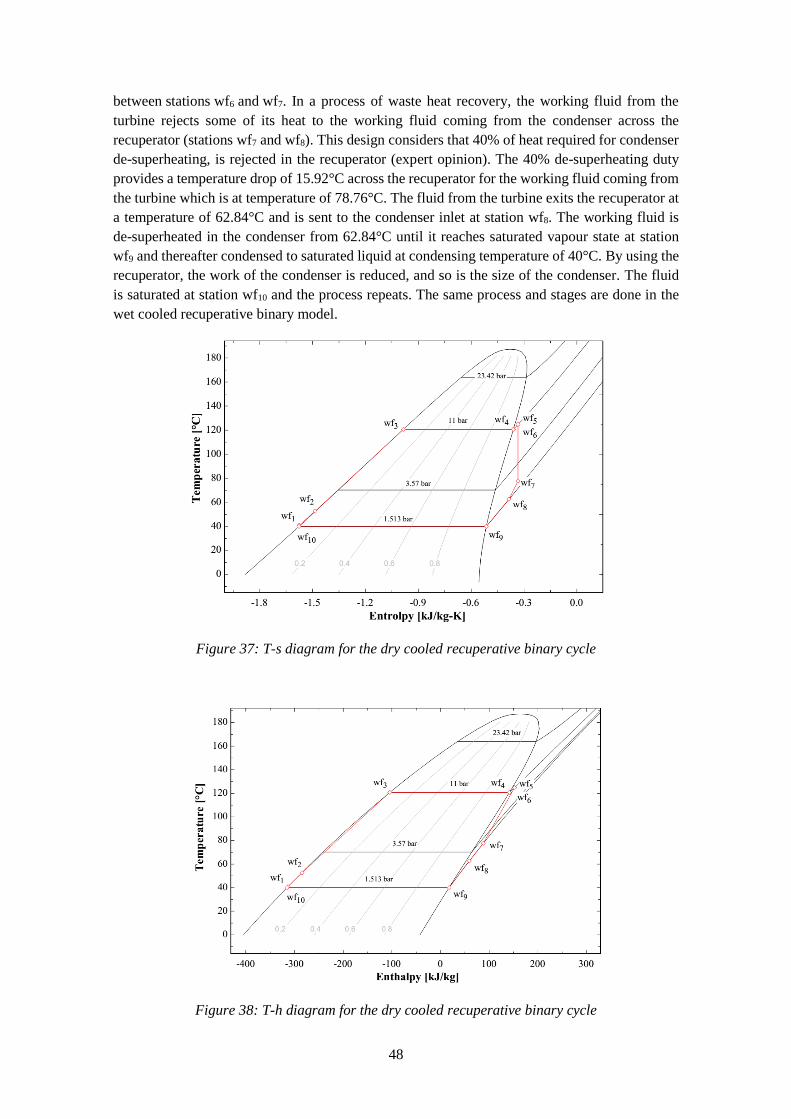
48
between stations wf6 and wf7. In a process of waste heat recovery, the working fluid from the
turbine rejects some of its heat to the working fluid coming from the condenser across the
recuperator (stations wf7 and wf8). This design considers that 40% of heat required for condenser
de-superheating, is rejected in the recuperator (expert opinion). The 40% de-superheating duty
provides a temperature drop of 15.92°C across the recuperator for the working fluid coming from
the turbine which is at temperature of 78.76°C. The fluid from the turbine exits the recuperator at
a temperature of 62.84°C and is sent to the condenser inlet at station wf8. The working fluid is
de-superheated in the condenser from 62.84°C until it reaches saturated vapour state at station
wf9 and thereafter condensed to saturated liquid at condensing temperature of 40°C. By using the
recuperator, the work of the condenser is reduced, and so is the size of the condenser. The fluid
is saturated at station wf10 and the process repeats. The same process and stages are done in the
wet cooled recuperative binary model.
Figure 37: T-s diagram for the dry cooled recuperative binary cycle
Figure 38: T-h diagram for the dry cooled recuperative binary cycle
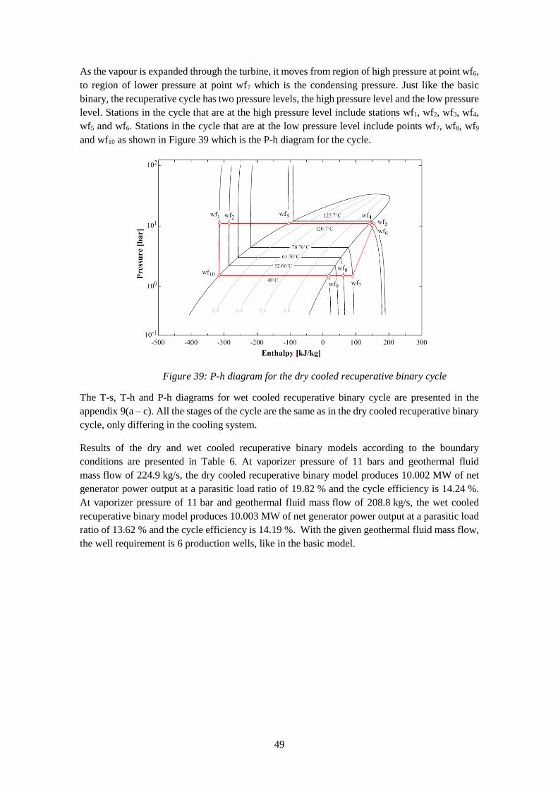
49
As the vapour is expanded through the turbine, it moves from region of high pressure at point wf6,
to region of lower pressure at point wf7 which is the condensing pressure. Just like the basic
binary, the recuperative cycle has two pressure levels, the high pressure level and the low pressure
level. Stations in the cycle that are at the high pressure level include stations wf1, wf2, wf3, wf4,
wf5 and wf6. Stations in the cycle that are at the low pressure level include points wf7, wf8, wf9
and wf10 as shown in Figure 39 which is the P-h diagram for the cycle.
Figure 39: P-h diagram for the dry cooled recuperative binary cycle
The T-s, T-h and P-h diagrams for wet cooled recuperative binary cycle are presented in the
appendix 9(a – c). All the stages of the cycle are the same as in the dry cooled recuperative binary
cycle, only differing in the cooling system.
Results of the dry and wet cooled recuperative binary models according to the boundary
conditions are presented in Table 6. At vaporizer pressure of 11 bars and geothermal fluid
mass flow of 224.9 kg/s, the dry cooled recuperative binary model produces 10.002 MW of net
generator power output at a parasitic load ratio of 19.82 % and the cycle efficiency is 14.24 %.
At vaporizer pressure of 11 bar and geothermal fluid mass flow of 208.8 kg/s, the wet cooled
recuperative binary model produces 10.003 MW of net generator power output at a parasitic load
ratio of 13.62 % and the cycle efficiency is 14.19 %. With the given geothermal fluid mass flow,
the well requirement is 6 production wells, like in the basic model.
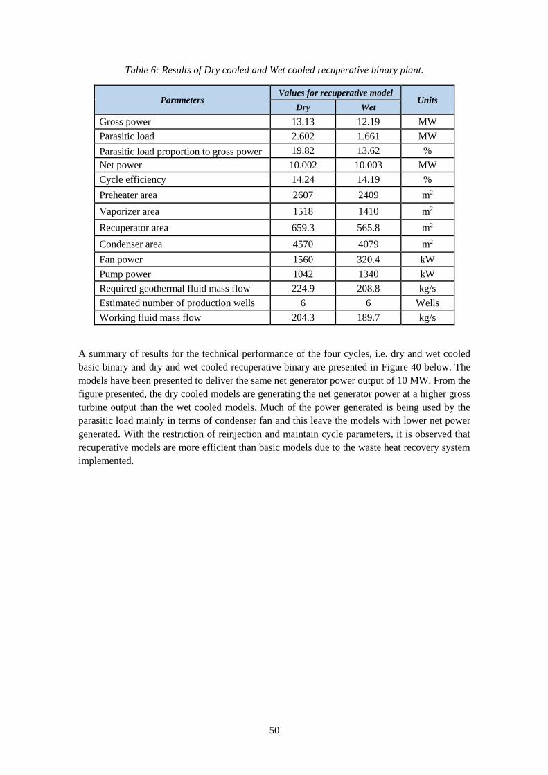
50
Table 6: Results of Dry cooled and Wet cooled recuperative binary plant.
Parameters Values for recuperative model
Units Dry Wet
Gross power 13.13 12.19 MW
Parasitic load 2.602 1.661 MW
Parasitic load proportion to gross power 19.82 13.62 %
Net power 10.002 10.003 MW
Cycle efficiency 14.24 14.19 %
Preheater area 2607 2409 m2
Vaporizer area 1518 1410 m2
Recuperator area 659.3 565.8 m2
Condenser area 4570 4079 m2
Fan power 1560 320.4 kW
Pump power 1042 1340 kW
Required geothermal fluid mass flow 224.9 208.8 kg/s
Estimated number of production wells 6 6 Wells
Working fluid mass flow 204.3 189.7 kg/s
A summary of results for the technical performance of the four cycles, i.e. dry and wet cooled
basic binary and dry and wet cooled recuperative binary are presented in Figure 40 below. The
models have been presented to deliver the same net generator power output of 10 MW. From the
figure presented, the dry cooled models are generating the net generator power at a higher gross
turbine output than the wet cooled models. Much of the power generated is being used by the
parasitic load mainly in terms of condenser fan and this leave the models with lower net power
generated. With the restriction of reinjection and maintain cycle parameters, it is observed that
recuperative models are more efficient than basic models due to the waste heat recovery system
implemented.
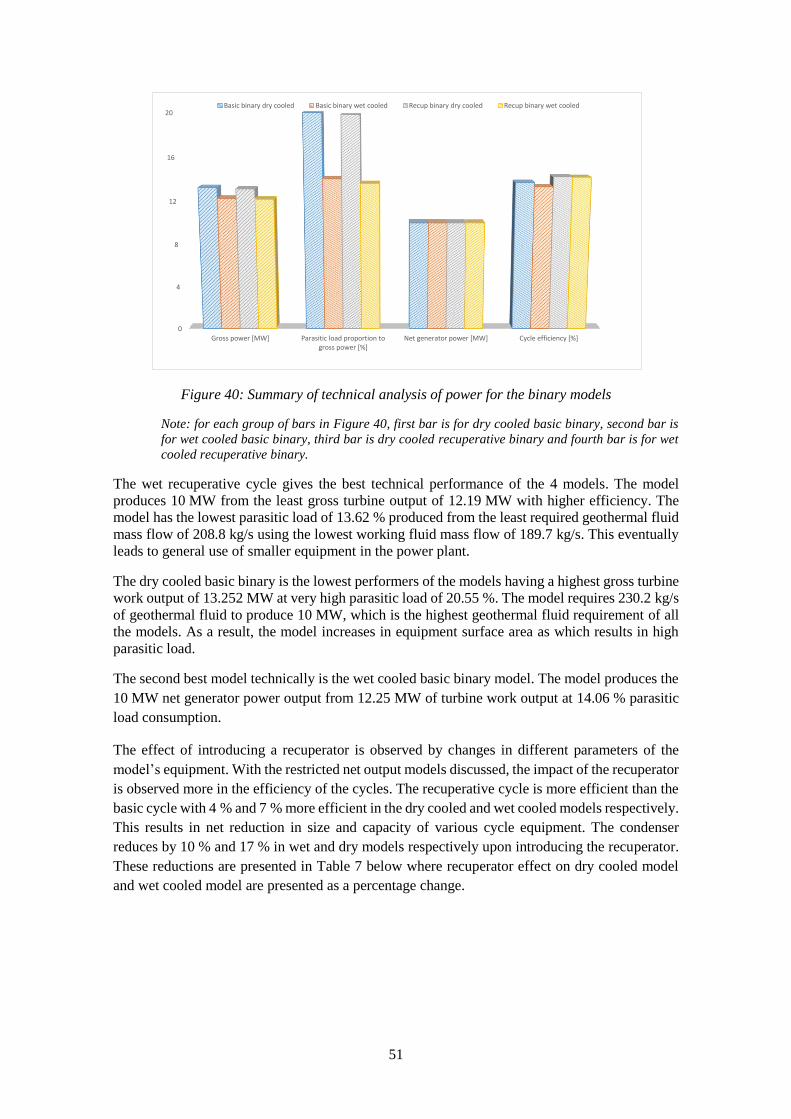
51
Figure 40: Summary of technical analysis of power for the binary models
Note: for each group of bars in Figure 40, first bar is for dry cooled basic binary, second bar is
for wet cooled basic binary, third bar is dry cooled recuperative binary and fourth bar is for wet
cooled recuperative binary.
The wet recuperative cycle gives the best technical performance of the 4 models. The model
produces 10 MW from the least gross turbine output of 12.19 MW with higher efficiency. The
model has the lowest parasitic load of 13.62 % produced from the least required geothermal fluid
mass flow of 208.8 kg/s using the lowest working fluid mass flow of 189.7 kg/s. This eventually
leads to general use of smaller equipment in the power plant.
The dry cooled basic binary is the lowest performers of the models having a highest gross turbine
work output of 13.252 MW at very high parasitic load of 20.55 %. The model requires 230.2 kg/s
of geothermal fluid to produce 10 MW, which is the highest geothermal fluid requirement of all
the models. As a result, the model increases in equipment surface area as which results in high
parasitic load.
The second best model technically is the wet cooled basic binary model. The model produces the
10 MW net generator power output from 12.25 MW of turbine work output at 14.06 % parasitic
load consumption.
The effect of introducing a recuperator is observed by changes in different parameters of the
model’s equipment. With the restricted net output models discussed, the impact of the recuperator
is observed more in the efficiency of the cycles. The recuperative cycle is more efficient than the
basic cycle with 4 % and 7 % more efficient in the dry cooled and wet cooled models respectively.
This results in net reduction in size and capacity of various cycle equipment. The condenser
reduces by 10 % and 17 % in wet and dry models respectively upon introducing the recuperator.
These reductions are presented in Table 7 below where recuperator effect on dry cooled model
and wet cooled model are presented as a percentage change.
0
4
8
12
16
20
Gross power [MW] Parasitic load proportion togross power [%]
Net generator power [MW] Cycle efficiency [%]
Basic binary dry cooled Basic binary wet cooled Recup binary dry cooled Recup binary wet cooled
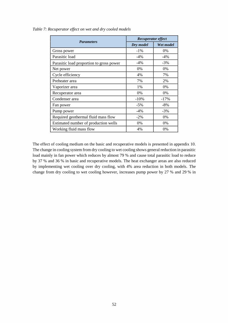
52
Table 7: Recuperator effect on wet and dry cooled models
Parameters Recuperator effect
Dry model Wet model
Gross power -1% 0%
Parasitic load -4% -4%
Parasitic load proportion to gross power -4% -3%
Net power 0% 0%
Cycle efficiency 4% 7%
Preheater area 7% 2%
Vaporizer area 1% 0%
Recuperator area 0% 0%
Condenser area -10% -17%
Fan power -5% -8%
Pump power -4% -3%
Required geothermal fluid mass flow -2% 0%
Estimated number of production wells 0% 0%
Working fluid mass flow 4% 0%
The effect of cooling medium on the basic and recuperative models is presented in appendix 10.
The change in cooling system from dry cooling to wet cooling shows general reduction in parasitic
load mainly in fan power which reduces by almost 79 % and cause total parasitic load to reduce
by 37 % and 36 % in basic and recuperative models. The heat exchanger areas are also reduced
by implementing wet cooling over dry cooling, with 4% area reduction in both models. The
change from dry cooling to wet cooling however, increases pump power by 27 % and 29 % in

53
basic and recuperative models respectively. Figure 41 below presents the change in equipment
size and mass flow of geothermal fluid as well as working fluid.
Figure 41: Comparison of equipment size and fluids for the binary models
0
500
1000
1500
2000
2500
3000
Preheater area Vaporizer
area
Recuperator
area
Condenser
area
Geothermal
fluid mass
flow
Working fluid
mass flow
Basic dry cooled Basic wet cooled Recup. dry cooled Recup. wet cooled
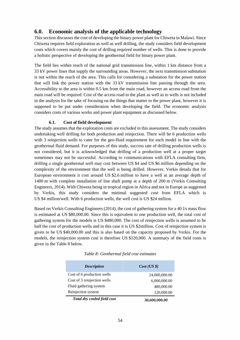
54
6.0. Economic analysis of the applicable technology This section discusses the cost of developing the binary power plant for Chiweta in Malawi. Since
Chiweta requires field exploration as well as well drilling, the study considers field development
costs which covers mainly the cost of drilling required number of wells. This is done to provide
a holistic perspective of developing the geothermal field for binary power plant.
The field lies within reach of the national grid transmission line, within 1 km distance from a
33 kV power lines that supply the surrounding areas. However, the next transmission substation
is not within the reach of the area. This calls for considering a substation for the power station
that will link the power station with the 33 kV transmission line passing through the area.
Accessibility to the area is within 0.5 km from the main road, however an access road from the
main road will be required. Cost of the access road to the plant as well as to wells is not included
in the analysis for the sake of focusing on the things that matter to the power plant, however it is
supposed to be put under consideration when developing the field. The economic analysis
considers costs of various works and power plant equipment as discussed below.
6.1. Cost of field development
The study assumes that the exploration costs are excluded in this assessment. The study considers
undertaking well drilling for both production and reinjection. There will be 6 production wells
with 3 reinjection wells to cater for the geo-fluid requirement for each model in line with the
geothermal fluid demand. For purposes of this study, success rate of drilling production wells is
not considered, but it is acknowledged that drilling of a production well at a proper target
sometimes may not be successful. According to communications with EFLA consulting firm,
drilling a single geothermal well may cost between US $4 and US $6 million depending on the
complexity of the environment that the well is being drilled. However, Verkis details that for
European environment it cost around US $2.6 million to have a well at an average depth of
1400 m with complete installation of line shaft pump at a depth of 200 m (Verkis Consulting
Engineers, 2014). With Chiweta being in tropical region in Africa and not in Europe as suggested
by Verkis, this study considers the minimal suggested cost from EFLA which is
US $4 million/well. With 6 production wells, the well cost is US $24 million.
Based on Verkis Consulting Engineers (2014), the cost of gathering system for a 40 l/s mass flow
is estimated at US $80,000.00. Since this is equivalent to one production well, the total cost of
gathering system for the models is US $480,000. The cost of reinjection wells is assumed to be
half the cost of production wells and in this case it is US $2million. Cost of reinjection system is
given to be US $40,000.00 and this is also based on the capacity proposed by Verkis. For the
models, the reinjection system cost is therefore US $120,000. A summary of the field costs is
given in the Table 8 below.
Table 8: Geothermal field cost estimates
Description Cost (US $)
Cost of 6 production wells 24,000,000.00
Cost of 3 reinjection wells 6,000,000.00
Fluid gathering system 480,000.00
Reinjection system 120,000.00
Total dry cooled field cost 30,600,000.00
55
The study assumes that the production wells will deliver as desired throughout the project life.
However, the reality is that production wells tend to decline in their fluid production as the
reservoir responds to the extraction of fluid. Such reservoir response calls for drilling of make-up
wells in order to maintain the production capacity of the power plant. Since reservoir
characteristics are not known at the moment, the assumption of constant well production of
geo-fluid holds.
6.2. Cost of power plant’s major equipment
The major components in the power plant are given in Table 9 below. The costs of the major
equipment are based on Ahangar (2012) and others where the unit costs of the equipment are
given as follows:
Vaporizer unit cost (US$/m2) 500
Preheater unit cost (US$/m2) 450
Recuperator unit cost (US$/m2) 600
Condenser unit cost (US$/m2) 400
Turbine unit cost (US$/kW) 500
Fan unit cost (US$/kW) 400
Pump unit cost (US$/kW) 450
The cost of wet cooling tower estimated as proposed by Forsha and Nichol is 170/kW (Forsha &
Nichols, 1992). When this cost is considered using inflation for the period 1992 – 2015, the
inflation consideration is 69.5% (BLS, 2015), the cost of cooling towers become enormous,
bearing in mind that improvements in technology have a bearing on costs. A model cooling tower
is created in cooling tower depot website, considering the required cooling water flow in the
cooling tower, based on model calculations, and the height of the tower. The cost of the modelled
cooling tower that satisfy the cooling requirements of the models and is made of fibre glass, is
US $936,138.00 (Cooling Tower Depot, 2015). This work rounds up the cooling tower cost to
US $1million.
The costs proposed by Ahangar (2012) are subjected to the inflation factor and used to calculate
indicative cost of major equipment according to their size and capacity and the cost of the
equipment is presented in Table 9.
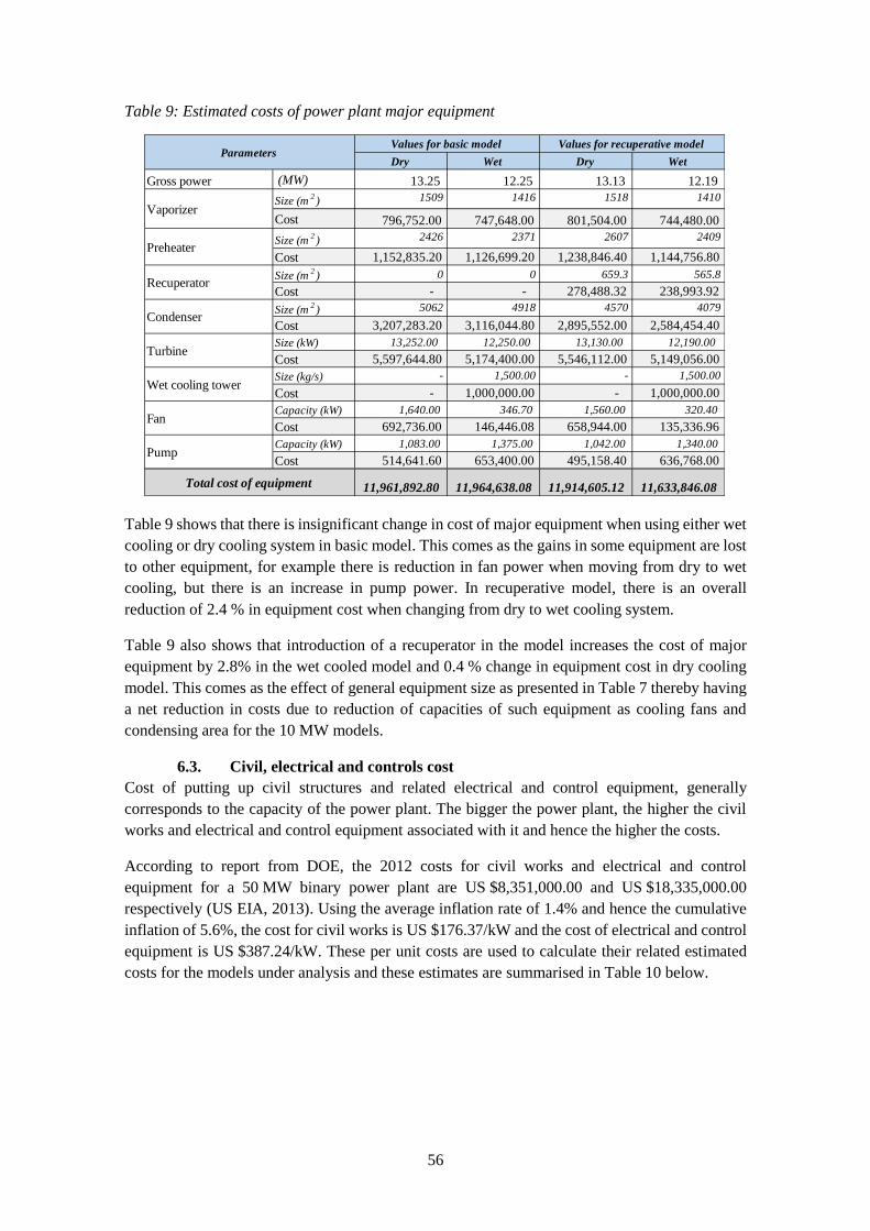
56
Table 9: Estimated costs of power plant major equipment
Table 9 shows that there is insignificant change in cost of major equipment when using either wet
cooling or dry cooling system in basic model. This comes as the gains in some equipment are lost
to other equipment, for example there is reduction in fan power when moving from dry to wet
cooling, but there is an increase in pump power. In recuperative model, there is an overall
reduction of 2.4 % in equipment cost when changing from dry to wet cooling system.
Table 9 also shows that introduction of a recuperator in the model increases the cost of major
equipment by 2.8% in the wet cooled model and 0.4 % change in equipment cost in dry cooling
model. This comes as the effect of general equipment size as presented in Table 7 thereby having
a net reduction in costs due to reduction of capacities of such equipment as cooling fans and
condensing area for the 10 MW models.
6.3. Civil, electrical and controls cost
Cost of putting up civil structures and related electrical and control equipment, generally
corresponds to the capacity of the power plant. The bigger the power plant, the higher the civil
works and electrical and control equipment associated with it and hence the higher the costs.
According to report from DOE, the 2012 costs for civil works and electrical and control
equipment for a 50 MW binary power plant are US $8,351,000.00 and US $18,335,000.00
respectively (US EIA, 2013). Using the average inflation rate of 1.4% and hence the cumulative
inflation of 5.6%, the cost for civil works is US $176.37/kW and the cost of electrical and control
equipment is US $387.24/kW. These per unit costs are used to calculate their related estimated
costs for the models under analysis and these estimates are summarised in Table 10 below.
Dry Wet Dry Wet
Gross power (MW) 13.25 12.25 13.13 12.19
Size (m2) 1509 1416 1518 1410
Cost 796,752.00 747,648.00 801,504.00 744,480.00
Size (m2) 2426 2371 2607 2409
Cost 1,152,835.20 1,126,699.20 1,238,846.40 1,144,756.80
Size (m2) 0 0 659.3 565.8
Cost - - 278,488.32 238,993.92
Size (m2) 5062 4918 4570 4079
Cost 3,207,283.20 3,116,044.80 2,895,552.00 2,584,454.40
Size (kW) 13,252.00 12,250.00 13,130.00 12,190.00
Cost 5,597,644.80 5,174,400.00 5,546,112.00 5,149,056.00
Size (kg/s) - 1,500.00 - 1,500.00
Cost - 1,000,000.00 - 1,000,000.00
Capacity (kW) 1,640.00 346.70 1,560.00 320.40
Cost 692,736.00 146,446.08 658,944.00 135,336.96
Capacity (kW) 1,083.00 1,375.00 1,042.00 1,340.00
Cost 514,641.60 653,400.00 495,158.40 636,768.00
11,961,892.80 11,964,638.08 11,914,605.12 11,633,846.08 Total cost of equipment
Values for basic model Values for recuperative model
Turbine
Vaporizer
Recuperator
Fan
Pump
Condenser
Preheater
Wet cooling tower
Parameters

57
Table 10: Summary of civil works and electrical and control equipment costs
6.4. Total costs of developing the models
All costs discussed are summarised in the Table 11 below. The table shows that wet cooled
recuperative binary is the least cost model in this assessment costing US $49.1 million, while the
dry cooled basic binary is the most expensive cycle in the analysis costing US $50 million. Wet
cooled basic binary model and dry cooled recuperative binary model come second and third
respectively as the least cost models with the wet cooled basic model being cheaper than the dry
cooled recuperative model at US $49.47 million and US $49.91 million respectively. A graphical
presentation of the total cost of the models is presented in the Figure 42 below.
Table 11: Total cost of developing the models
Figure 42: Total cost of models
From US EIA (2013)
Inflation 2013 to 2015
Capacity (kW) 50,000
Civil works cost (US$) 8,351,000.00
Electrical & control equipment cost (US$) 18,335,000.00
Dry Wet Dry Wet
Civil works cost 2,337,296.59 2,160,570.72 2,315,779.07 2,149,988.33
Electrical & control equipment cost 5,131,640.87 4,743,631.20 5,084,398.18 4,720,397.09
DescriptionValues for basic model (US$) Values for recuperative model (US$)
Per kW cost Inflation Corrected
106%
176.37
387.24
Dry Wet Dry Wet
Field development 30,600,000.00 30,600,000.00 30,600,000.00 30,600,000.00
Major equipment cost 11,961,892.80 11,964,638.08 11,914,605.12 11,633,846.08
Civil works cost 2,337,296.59 2,160,570.72 2,315,779.07 2,149,988.33
Electrical & control equipment cost 5,131,640.87 4,743,631.20 5,084,398.18 4,720,397.09
Total cost without field development 19,430,830.26 18,868,840.00 19,314,782.36 18,504,231.50
Grand total project cost 50,030,830.26$ 49,468,840.00$ 49,914,782.36$ 49,104,231.50$
DescriptionValues for basic model (US$) Values for recuperative model (US$)
$50,030,830.26
$49,468,840.00
$49,914,782.36
$49,104,231.50
BASIC BINARY DRY
COOLED
BASIC BINARY WET
COOLED
RECUPERATIVE
BINARY DRY COOLED
RECUPERATIVE
BINARY WET COOLED
Power plant cost
(US $)
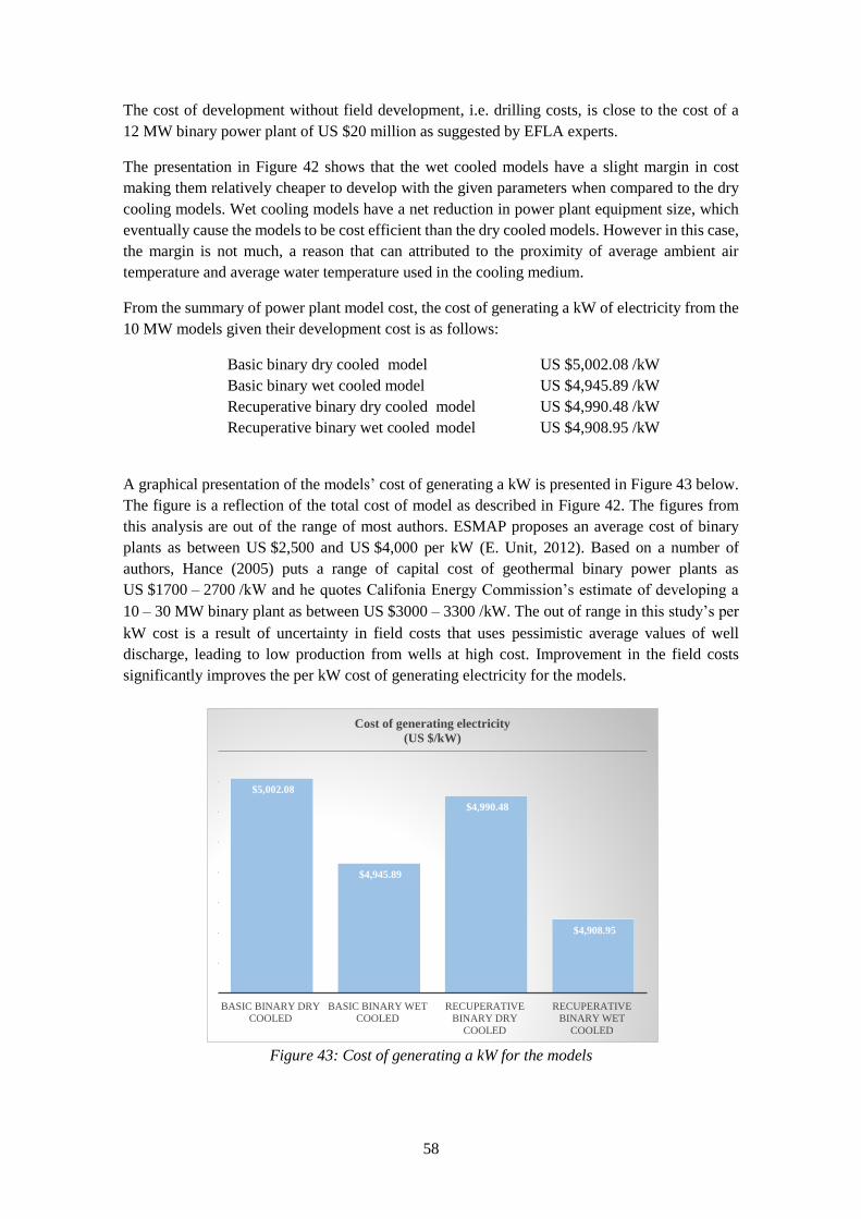
58
The cost of development without field development, i.e. drilling costs, is close to the cost of a
12 MW binary power plant of US $20 million as suggested by EFLA experts.
The presentation in Figure 42 shows that the wet cooled models have a slight margin in cost
making them relatively cheaper to develop with the given parameters when compared to the dry
cooling models. Wet cooling models have a net reduction in power plant equipment size, which
eventually cause the models to be cost efficient than the dry cooled models. However in this case,
the margin is not much, a reason that can attributed to the proximity of average ambient air
temperature and average water temperature used in the cooling medium.
From the summary of power plant model cost, the cost of generating a kW of electricity from the
10 MW models given their development cost is as follows:
Basic binary dry cooled model US $5,002.08 /kW
Basic binary wet cooled model US $4,945.89 /kW
Recuperative binary dry cooled model US $4,990.48 /kW
Recuperative binary wet cooled model US $4,908.95 /kW
A graphical presentation of the models’ cost of generating a kW is presented in Figure 43 below.
The figure is a reflection of the total cost of model as described in Figure 42. The figures from
this analysis are out of the range of most authors. ESMAP proposes an average cost of binary
plants as between US $2,500 and US $4,000 per kW (E. Unit, 2012). Based on a number of
authors, Hance (2005) puts a range of capital cost of geothermal binary power plants as
US $1700 – 2700 /kW and he quotes Califonia Energy Commission’s estimate of developing a
10 – 30 MW binary plant as between US $3000 – 3300 /kW. The out of range in this study’s per
kW cost is a result of uncertainty in field costs that uses pessimistic average values of well
discharge, leading to low production from wells at high cost. Improvement in the field costs
significantly improves the per kW cost of generating electricity for the models.
Figure 43: Cost of generating a kW for the models
$5,002.08
$4,945.89
$4,990.48
$4,908.95
BASIC BINARY DRY
COOLED BASIC BINARY WET
COOLED RECUPERATIVE
BINARY DRY
COOLED
RECUPERATIVE
BINARY WET
COOLED
Cost of generating electricity
(US $/kW)
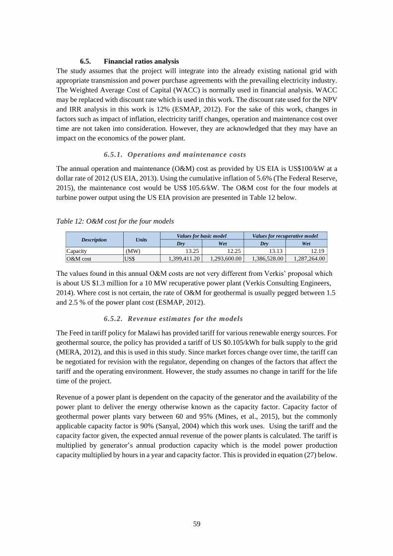
59
6.5. Financial ratios analysis
The study assumes that the project will integrate into the already existing national grid with
appropriate transmission and power purchase agreements with the prevailing electricity industry.
The Weighted Average Cost of Capital (WACC) is normally used in financial analysis. WACC
may be replaced with discount rate which is used in this work. The discount rate used for the NPV
and IRR analysis in this work is 12% (ESMAP, 2012). For the sake of this work, changes in
factors such as impact of inflation, electricity tariff changes, operation and maintenance cost over
time are not taken into consideration. However, they are acknowledged that they may have an
impact on the economics of the power plant.
6.5.1. Operations and maintenance costs
The annual operation and maintenance (O&M) cost as provided by US EIA is US$100/kW at a
dollar rate of 2012 (US EIA, 2013). Using the cumulative inflation of 5.6% (The Federal Reserve,
2015), the maintenance cost would be US$ 105.6/kW. The O&M cost for the four models at
turbine power output using the US EIA provision are presented in Table 12 below.
Table 12: O&M cost for the four models
The values found in this annual O&M costs are not very different from Verkis’ proposal which
is about US $1.3 million for a 10 MW recuperative power plant (Verkis Consulting Engineers,
2014). Where cost is not certain, the rate of O&M for geothermal is usually pegged between 1.5
and 2.5 % of the power plant cost (ESMAP, 2012).
6.5.2. Revenue estimates for the models
The Feed in tariff policy for Malawi has provided tariff for various renewable energy sources. For
geothermal source, the policy has provided a tariff of US $0.105/kWh for bulk supply to the grid
(MERA, 2012), and this is used in this study. Since market forces change over time, the tariff can
be negotiated for revision with the regulator, depending on changes of the factors that affect the
tariff and the operating environment. However, the study assumes no change in tariff for the life
time of the project.
Revenue of a power plant is dependent on the capacity of the generator and the availability of the
power plant to deliver the energy otherwise known as the capacity factor. Capacity factor of
geothermal power plants vary between 60 and 95% (Mines, et al., 2015), but the commonly
applicable capacity factor is 90% (Sanyal, 2004) which this work uses. Using the tariff and the
capacity factor given, the expected annual revenue of the power plants is calculated. The tariff is
multiplied by generator’s annual production capacity which is the model power production
capacity multiplied by hours in a year and capacity factor. This is provided in equation (27) below.
Dry Wet Dry Wet
Capacity (MW) 13.25 12.25 13.13 12.19
O&M cost US$ 1,399,411.20 1,293,600.00 1,386,528.00 1,287,264.00
Description UnitsValues for basic model Values for recuperative model
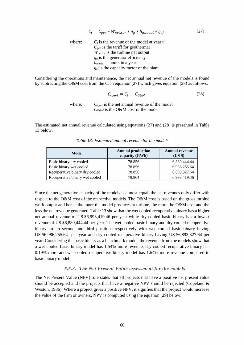
60
𝐶𝑡 = 𝐶𝑔𝑒𝑜 ∗ 𝑊𝑛𝑒𝑡.𝑡𝑢𝑟 ∗ 𝜂𝑔 ∗ ℎ𝑎𝑛𝑛𝑢𝑎𝑙 ∗ 𝜂𝑐𝑓 (27)
where: Ct is the revenue of the model at year t
Cgeo is the tariff for geothermal
Wnet.tur is the turbine net output
ηg is the generator efficiency
hannual is hours in a year
ηcf is the capacity factor of the plant
Considering the operations and maintenance, the net annual net revenue of the models is found
by subtracting the O&M cost from the Ct in equation (27) which gives equation (28) as follows:
𝐶𝑡_𝑛𝑒𝑡 = 𝐶𝑡 − 𝐶𝑂&𝑀 (28)
where: Ct_net is the net annual revenue of the model
CO&M is the O&M cost of the model
The estimated net annual revenue calculated using equations (27) and (28) is presented in Table
13 below.
Table 13: Estimated annual revenue for the models
Model Annual production
capacity (GWh)
Annual revenue
(US $)
Basic binary dry cooled 78.856 6,880,444.44
Basic binary wet cooled 78.856 6,986,255.64
Recuperative binary dry cooled 78.856 6,893,327.64
Recuperative binary wet cooled 78.864 6,993,419.46
Since the net generation capacity of the models is almost equal, the net revenues only differ with
respect to the O&M cost of the respective models. The O&M cost is based on the gross turbine
work output and hence the more the model produces at turbine, the more the O&M cost and the
less the net revenue generated. Table 13 show that the wet cooled recuperative binary has a higher
net annual revenue of US $6,993,419.46 per year while dry cooled basic binary has a lowest
revenue of US $6,880,444.44 per year. The wet cooled basic binary and dry cooled recuperative
binary are in second and third positions respectively with wet cooled basic binary having
US $6,986,255.64 per year and dry cooled recuperative binary having US $6,893,327.64 per
year. Considering the basic binary as a benchmark model, the revenue from the models show that
a wet cooled basic binary model has 1.54% more revenue, dry cooled recuperative binary has
0.19% more and wet cooled recuperative binary model has 1.64% more revenue compared to
basic binary model.
6.5.3. The Net Present Value assessment for the models
The Net Present Value (NPV) rule states that all projects that have a positive net present value
should be accepted and the projects that have a negative NPV should be rejected (Copeland &
Weston, 1986). Where a project gives a positive NPV, it signifies that the project would increase
the value of the firm or owners. NPV is computed using the equation (29) below:

61
𝑁𝑃𝑉 = −𝐶0 + ∑
𝐶𝑡_𝑛𝑒𝑡
(1 + 𝑟)𝑡
𝑁
𝑡=1
(29)
where: t is the annual time of the project
N is the life time of the project
-C0 is the initial capital of the project
r is the cost of capital (discount rate).
The life time of the project is set for 20 years at the discount rate of 12%. Using equation (29) the
NPV for the models are calculated and presented in Figure 44 below.
Figure 44: Net Present Value for the models
It is observed from Figure 44 that all the models have positive NPV for the 20 years life time of
assessment. The model with the least NPV is the dry cooled basic binary with US $1.36 million
and the model with the highest NPV is the wet cooled recuperative binary with US $3.13 million
which is 130 %% more than the least NPV model. The wet cooled basic binary has an NPV of
US $2.71 million which is 99.27 %% more as compared to the least NPV model, while the dry
cooled recuperative binary has an NPV of US $1.57 million representing a 15.58 % more than the
least NPV model. For mutually exclusive projects, a decision is usually based on an investment
with the higher NPV. In this case the wet cooled recuperative binary would be considered.
6.5.4. The Internal Rate of Return
The internal rate of return (IRR) is a discount rate of a project which equates the present value of
the project’s cash outflows and inflows or equates a project's investment in a certain time period
with its cash inflows. In other words, IRR is the rate at which the project's NPV is zero (Copeland
& Weston, 1986) i.e. where the project can break even. Hence this is the rate of return on invested
capital that the project is returning to the firm. The IRR helps to assess profitability of the project
and is found by using equation (30) as shown below.
𝐶0 = + ∑
𝐶𝑡_𝑛𝑒𝑡
(1 + 𝑟𝑖)𝑡
𝑁
𝑡=1
(30)
where: 𝑟𝑖 is the internal rate of return (IRR)
The initial guess rate for this analysis assumes the given discount rate for NPV analysis above.
There is a relationship between the IRR and the opportunity cost of alternative capital investment
project. IRR is associated with the expected rate of return from the project such that if the result
$1,362,261.60
$2,714,602.65
$1,574,539.83
$3,132,720.90
$- $500,000.00 $1,000,000.00 $1,500,000.00 $2,000,000.00 $2,500,000.00 $3,000,000.00 $3,500,000.00
NP
V (
US
$)
Recuperative binary wet cooled Recuperative binary dry cooled Basic binary wet cooled Basic binary dry cooled

62
of IRR is more than the expected return, the investment is acceptable. Otherwise the investment
is rejected if the value of IRR is less than expected rate of return. It also goes that the higher the
IRR for a project, the better the project is economically.
Using equation (30) and the initial guess rate of 12 as in discount rate, the IRR for the 4 models
is computed and the results are given in Table 14.
Table 14: Internal Rate of Return for the models
Model IRR (%)
Basic binary dry cooled 12.43%
Basic binary wet cooled 12.87%
Recuperative binary dry cooled 12.50%
Recuperative binary wet cooled 13.01%
The results of IRR follow the NPV trend, with slim margins between the models. The wet cooled
recuperative model has a highest IRR of 13.01 %, dry cooled basic model has the lowest IRR of
12.43 %. The wet cooled basic model has an IRR of 12.87 % which is close to the highest, and
dry cooled basic model has an IRR of 12.50 %. With the rule of the bigger the better, the wet
cooled recuperative model would also be considered in this analysis. The results of IRR are
similar to the results from a hypothetical 50 MW geothermal power plant as presented by ESMAP
(2012), which is 13.4% at a tariff of US $0.12 /kWh for 30 years.
6.5.5. Discounted Payback Period
In this analysis, the discounted annual revenue are used to give an indication of how soon the
model can recover its investment i.e. estimating the years to recover the initial capital investment.
The traditional payback period does not account for the time value for money thereby providing
not so realistic estimate of investment recovery as the discounted method does. Discounted
payback period incorporates time value for money by discounting all the future revenue of the
project thereby providing a better estimate of how long the project would recover its initial
investment.
The discount payback period is a sum of all discounted future revenues and the initial investment.
The initial investment is a negative value while all revenues are positive values. The year that the
sum of investment and revenue becomes a positive, is the payback period. The discount rate used
in this analysis is the same as used in NPV. The discounted payback period is presented in Figure
45 below.
From Figure 45, wet cooled recuperative binary and wet cooled basic binary models have early
discounted payback period in the 17th year. The two models are followed by dry cooled
recuperative model in year 18 and lastly the dry cooled basic model in year 19. The discounted
payback period is sensitive to the discount rate and the tariff of electricity in such a way that with
higher discount rate, the payback period gets longer while with lower discount rates the models
have a shorter payback period. In terms of tariff, the higher the tariff, the shorter the payback
period and the lower the tariff, the longer the payback period.
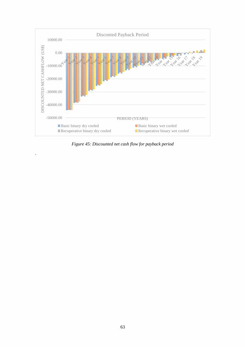
63
Figure 45: Discounted net cash flow for payback period
.
-50000.00
-40000.00
-30000.00
-20000.00
-10000.00
0.00
10000.00D
ISC
OU
NT
ED
NE
T C
AS
HF
LO
W (
US
$)
PERIOD (YEARS)
Disconted Payback Period
Basic binary dry cooled Basic binary wet cooled
Recuperative binary dry cooled Recuperative binary wet cooled
64
7.0. Conclusion The East African Rift System is the major source of geothermal power in Africa. The system is
divided into three branches, the eastern branch, western branch and the south eastern branch. The
eastern branch is more active with volcanoes. Many studies have been done to understand the
branch which has high temperature resource and hence more high temperature utilization projects
have been developed. The western branch is paucity of volcanoes and is relatively cooler when
compared to the eastern branch. Limited number of studies have been carried out and hence there
is less understanding of this branch. With lower temperatures, mostly below 200°C, estimated
along the western branch and considering the Lindal diagram of geothermal utilization, it is
recommended that geothermal electricity production projects along the branch be of binary type
unless substantial detailed studies prove otherwise. Malawi being within the western branch of
the EARS and not showing surface manifestations of high temperature system, should consider
developing its resource for electricity using binary power plant technology.
Four models of binary technology can be applicable for Chiweta geothermal field in Malawi,
which are wet cooled basic binary, dry cooled basic binary, wet cooled recuperative binary and
dry cooled recuperative binary. The four models have been subjected to technical and economic
analysis using available data and literature based assumptions wherever necessary.
The differences in the technical performance of the models are attributed to use of either air or
water as a cooling medium in the models’ condensers as well as introducing a recuperator as a
waste heat recovery system.
Wet cooled models are observed to operate much better than the dry cooled models in terms of
equipment size at the same net power generation. The impact of the cooling medium on
performance is such that air is less dense than water and therefore would require more volume of
air to cool the same amount of working fluid at a given temperature range which less volume of
water would do. The specific heat capacity for air is much less compared to the specific heat
capacity of water making wet cooling systems more efficient that dry cooling systems. This then
translates into more surface area for condensing in a dry cooling system than in wet cooling
system. The models show a decrease in condenser area by 3 % in basic models and by 11 % in
recuperative models due to cooling system. Due to the nature of air, more parasitic load is
demanded by fans to push the volume of the cooling medium across the condenser in the dry
cooling system thereby presenting less net power output than in wet cooling system. The models
show a 37 % and 36 % reduction in parasitic load in basic and recuperative models respectively.
The introduction of recuperator in the models provides an improvement in efficiency of the cycle
with reduction in parasitic load. The recuperative cycle is more efficient than the basic cycle with
4 % and 7 % more efficient in the dry cooled and wet cooled models respectively. This results in
net reduction in size and capacity of various cycle equipment. The most noted change in size is
the condenser that reduces by 10 % in dry models and by 17 % in wet models.
The differences in the economic performance of the models are attributed mainly to the size of
equipment as demanded by the models. The technical analysis reveals that dry cooled models
require larger cooling and parasitic load equipment to do a similar job that wet cooled model
equipment would do thereby affecting the model’s efficiency as well as demanding more
geothermal fluid than the wet cooled models. This eventually leads to higher capital cost as well
as lower revenue when compared to the wet cooling system with the same primary cycle
conditions. The model with the lowest cost of power plant is the wet cooled recuperative binary

65
costing US $49.1 million. The second lowest cost model is the wet cooled basic binary which is
0.7 % more costly as compared to wet cooled recuperative model. The third least cost model is
the dry cooled recuperative binary with 1.65 % and the most expensive model of the dry cooled
basic binary at 1.89 % more than the wet cooled recuperative model.
All the models have a positive Net Present Value when analysed using a discount rate of 12 %.
The best NPV is from wet cooled recuperative binary with US $3.1 million followed by wet
cooled basic binary with US $2.7 million. All the models give a satisfactory Internal Rate of
Return which is more than the discount rate used in the NPV. The wet cooled recuperative model
gives the best IRR of 13 % while the least IRR is 12.43 % for dry cooled basic binary. Using
discounted revenue, the earlies discounted payback period for the models is from wet cooled
recuperative model and wet cooled basic model in 17th year followed by dry cooled recuperative
model in year 18 and finally the dry cooled basic model in year 19.
The results of the analysis show that the best model for implementation is the wet cooled
recuperative binary with respect to both technical and economic performance. With a gross power
of 12.19 MW the wet cooled recuperative model produces 10 MW of net generator power output
using parasitic load of 13.62 % and at cycle efficiency of 14.19 %. The model is 8 % better in
turbine work output and 39 % better in parasitic load consumption when compared to the least
technical performer.
With per capita consumption of 93kWh, generating 10MW from geothermal for Malawi would
serve up to 900,000 people or 180,000 households assuming a household of 5 people. The country
is still below the recommended sub-Saharan per-capita rate of 432kWh let alone the world’s
recommended average per capita rate of 2167kWh (Taulo, et al., 2015), therefore any additional
MW for the people matters for the country to improve on its per capita consumption.

66
8.0. Recommendations The study has shown that a wet cooled recuperative binary is the best in both technical and
economic analysis. The analysis has included challenges of silica scaling potential in geothermal
fluid hence consideration minimum reinjection temperature to avoid silica scaling. Usually the
purpose of including a recuperator in a cycle is to improve cycle efficiency where waste heat is
recovered leading to less extraction of heat from the source fluid (Valdimarsson, 2010). In
geothermal, this helps in case where source fluid presents high potential of silica scaling driven
by fluid chemistry. The recuperator helps to improve the reinjection temperature. However, the
inclusion of a recuperator which is another heat exchanger, introduces additional pressure loss at
the turbine exit leading to reduction in power output as the turbine exit operates at higher pressure
than in a case without a recuperator. Without considering pressure drops in heat exchangers, the
determined reinjection temperature for this study shows that working with a wet cooled basic
binary achieves almost the same results as the wet cooled recuperative model. This would mean
that incorporating heat exchanger pressure losses in the models would introduces more pressure
instabilities in the recuperative model than the basic model. This work therefore recommends
implementation of a wet cooled basic binary model as the most ideal model for Chiweta
geothermal field in Malawi. The recommended model comes second to the wet cooled
recuperative model in both technical and economic analysis with small differences such as
producing 10 MW at 14.06 % parasitic load unlike 13.62 % for the wet cooled recuperative. Per
kW cost of production of wet cooled basic binary is 0.74 % more than the wet cooled recuperative,
meaning their cost is almost the same but would differ in terms of cycle stability in light of
pressure drops in heat exchangers. The total cost of wet cooled basic binary is US $49.5 million
which can be recovered in 17 years. Further studies that include pressure drops in the heat
exchangers are recommended.
With emerging technologies, the fluid at temperature of 180°C, may be flashed and the flashed
steam used for vaporizing the working fluid while the liquid used for preheating. Depending on
the actual characteristics of the field this model may be further analysed if it can be applicable for
Chiweta. The analysis may also dwell on incorporating a flash plant to use the steam and the
binary in the event that Chiweta field proves to be much better for just a binary plant.
Binary cycle plants use flammable working fluids as discussed in the choice of working fluid
section. This study has not included safety and mitigation of the working fluid in an emergency.
Further studies are recommended to incorporate technical requirements for fire-fighting
equipment and their cost implications to the model.
It is also recommended for more resource assessment studies to be done for the Chiweta field,
especially sub surface studies, in order to obtain real data for a better model of a power plant to
be implemented. This will assist in improving the models in such areas as restriction of reinjection
temperature where more energy can be extracted from the resource for utilization.
The recommended model will use water from either Lake Malawi or the North Rumphi River.
The proposed area of the model has settlements within the vicinity that would be affected by the
development of the model. As such, it is recommended that a detailed Environmental Impact
Assessment (EIA) for developing the model be considered prior to model development as required
by the Environmental Act of Malawi. This will ensure that appropriate mitigation measures in the
form of Environmental Management Plan be developed, addressing any impacts that may arise
from developing the model in the area.
67
9.0. References Ahangar, F., 2012. Feasibilty Study of Developing a Binary Power Plant in the Low-
Temperature Geothermal Field in Puga, Jammu and Kashmir, India., Reykjavik,
Iceland: UNU-GTP.
Ashwood, A. & Bharathan, D., 2011. Hybrid Cooling Systems for Low-Temperature
Geothermal Power Production, Colorado, USA: NREL.
Bao, J. & Zhao, L., 2013. A review of working fluid and expander selections for organic
Rankine cycle. Renewable and Sustainable Energy review, pp. 325-342.
Bertani, R., 2010. Geothermal power generation in the world, 2005–2010, update report.. Bali,
Indonesia, IGA.
BLS, 2015. Bureau of Labour Statistics, United Stated Department of Labour. [Online]
Available at: http://www.bls.gov/data/inflation_calculator.htm
[Accessed 04 December 2015].
Brown, K., 2013. Mineral Scaling in Geothermal Power Production. Reykjavik, Iceland: UNU-
GTP.
Chorowicz, J., 2005. The East African rift system. Journal of African Earth Science, pp. 379-
410.
Climate Data, 2015. [Online]
Available at: http://en.climate-data.org/location/207402/
ClimaTemps.com, 2015. Karonga climatemp. [Online]
Available at: http://www.karonga.climatemps.com/humidity.php
Cooling Tower Depot, 2015. Cooling Tower Optimization. [Online]
Available at: https://www.coolingtowerdepot.com/content/depot/cooling-tower-
optimization
[Accessed 10 12 2015].
Copeland, T. & Weston, J., 1986. Financial Theory and Corporate Policy.. Reading,
Massachusetts.: Addison-Wesley.
Cordova Geirdal, C., Gudjonsdottir, M. & Jensson, P., 2015. Economic comparison of a well-
head geothermal power plant and a traditional one. Geothermics, pp. 1-13.
Dickson, M. & Fanell, M., 2003. Geothermal Energy: Utilization and Technology. Paris,
France: UNESCO.
DiPippo, R., 1985. A simplified method for estimating the silica scaling potential in geothermal
power plants. Geothermal Resources Council, Bulletin, May, pp. 3-9.
DiPippo, R., 1999. Small Geothermal Power Plants: Design, Performance and Economic.. Geo-
Heat Center Bulletin, June.
DiPippo, R., 2012. Geothermal Power Plants: Principles, Applications, Case Studies and
Environmental Impact, 3rd. Edition. Oxford, UK: Elsevier.

68
DoE, 2003. National Energy Policy of Malawi - Department of Energy Affairs. Zomba, Malawi:
Government Printers, Malawi Government.
Dulanya, Z., Morales-Simfors, N. & Sivertun, A., 2010. A Comparison Between Silica and
Cation Geothermometry of the Malawi Hotsprings. Bali, Indonesia, s.n.
E. Unit, 2012. Drilling Down on Geothermal Potential: An Assessment for Central America,
s.l.: ESMAP, World Bank..
Eliasson, E., Thorhallsson, S. & Steingrimsson, B., 2008. Geothermal Power Plants. Entebbe,
Uganda, UNU-GTP.
Eliyasi, C., 2015. MSc. Thesis report: Geothermal Potential Mapping of Northern Malawi
Using Remote Sensig and Geological Data Intergration, Enschede, Netherlands:
University of Twente.
ESMAP, 2012. Geothermal Handbook: P,anning and Financing Power Generation,
Washington DC, USA: World Bank Group.
Forsha, M. D. & Nichols, K. E., 1992. Factors affecting the capital cost of binary power plants..
Geothermal Resources Council BULLETIN, August, pp. 261-264.
Fournier, R. & Rowe, J., 1977. The solubility of amorphous silica in water at high temperatures
and high pressures. Amerian Mineralogist , pp. 1052 - 1056.
Frick, S., Kranz, S. & Saadat, A., 2015. Improving the Annual Net Power Output of Geothermal
Binary Power Plants.. Melbourne, Australia, IGA.
GDC - Kenya, 2010. Assessment of the Geothermal Potential of Malawi (Unpublished),
Lilongwe, Malawi: Geothermal Development Company - Kenya report prepared for
Geothermal Projects Limited.
Gondwe, K. et al., 2012. Geothermal Development in Malawi – a Country Update. Proceedings
at 4th African Rift Geothermal Conference - Nairobi, Kenya, 21-23 November, 2012.
Hance, C., 2005. Factors Affecting Costs of Geothermal Power Development, Washington D.C.:
Geothermal Energy Association.
Hardarson, B., 2014. Structural Geology of the Western Branch of the East African Rift:
Tectonics, Vlcanology and Geothermal Activity.. Naivasha, Kenya, UNU-GTP.
Hettiarachchi, H., Golubovic, M., Worek, W. & Ikegami, Y., 2007. Optimum design criteria for
an Organic Rankine cycle using low-temperature geothermal heat sources. Energy,
September, pp. 1698 - 1706.
Kraml, M., Mnjokava, T., Mayalla, J. & Kabaka, K., 2010. Surface Exploration of a Viable
Geothermal Resource in Mbeya Area, SW Tanzania. Part II: Geochemistry.. Bali,
Indonesia, IGA.
Leeper, S., 1981. Wet Cooling Towers: 'Rule of thumb' Design and Simulation , Idaho, USA:
US Department of Energy.

69
Maghiar , T. & Antal, C., 2001. Power Generation from Low-Enthalpy Geothermal Resources.
GeoHeat Center Bulletin, June, pp. 35-37.
Mannvit - Geoelec, 2012. Working paper: A Software to evaluate financial viability of
geothermal projects., Reykjavik, Iceland: s.n.
Marcuccilli, F. & Thiolet, D., 2010. Optimizing Binary Cycles Thanks to Radial Inflow
Turbines. Bali, Indonesia, IGA.
Mburu, M., 2013. Geothermal Energy Utilization. Naivasha, Kenya, UNU-GTP.
MCC-Malawi, 2015. Investment Outlook - Business Opportunities in the Malawi Power Sector,
Lilongwe, Malawi: Millenium Challenge Corporation.
Mdala, H., 2015. MSc. Thesis report: Determining Structural Variations Between the Northern
and Southern Provinces of the Malawi Rift By Using Automatic Lineament Extraction
Method., Enschede, Netherlands: University of Twente.
Mendrinos, D., Kontoleontos, E. & Karytsas, C., 2006. Geothermal Binary Plants: Water or Air
Cooled?. Strasbourg, France, s.n.
MERA, 2012. Malawi Feed-In Tariff Policy, Lilongwe, Malawi: Malawi Energy Regulatory
Authority .
Mines, G. et al., 2015. Geothermal Plant Capacity Factors. Stanford, California, Stanford
University.
Mlcak, H., 2002. Kalina Cycle Concepts for Low Temperature Geothermal. Geothermal
Resource Council, pp. 707-713.
Mwagomba, T., 2013. Comparative Analysis of Geothermal Power Plant Designs Suitable for
Malawi's Chiweta Geothermal Field.. In: Geothermal Training in Iceland: 2013.
Reykjavik, Iceland.: UNU-GTP.
NSO, 2010. Population Projection Malawi, Zomba, Malawi: National Statistical Office.
Nugroho, A., 2011. Optimization of electrical power production from high temperature
geothermal fields with respect to silica scaling problems, Reykjavik, Iceland: UNU-
GTP.
Omenda, P., 2013. The Geology and Geothermal Activity of the East African Rift.. Naivasha,
Kenya, UNU-GTP.
Pritchett, J., 1996. A study of electrical generating capacities of self-discharging slim holes.
Stanford, California., Stanford University, pp. 55-66.
Programme U, 2015. Encyclopedia of Earth, Lake Malawi. [Online]
Available at: http://www.eoearth.org/view/article/154128
Quinlivan, P. et al., 2015. Assessing Geothermal Tariffs in the Face of Uncertainty, a
Probabilistic Approach. Melbourne, Australia, IGA.
Ragnarsson, A., 2006. Geothermal utilization, direct use and power generation.. Nicaragua, s.n.

70
Saemundsson, K., Axelsson, G. & Steingrimsson, B., 2011. Geothermal Systems in Global
Perspective. Santa Tecla, El Salvador, UNU-GTP, p. 13.
Saleh, B., Koglbauer, G., Wendland, M. & Fischer, J., 2007. Working fluids for low-
temperature organic Rankine cycles. Energy, pp. 1210-1221.
Sanyal, S., 2004. Cost of Geothermal Power and Factors that Affect It. Stanford, Califonia,
Stanford University.
Simiyu, S., 2010. Status of Geothermal Exploration in Kenya and Future Plans for Its
Development. Bali, Indonesia, IGA.
Taulo, J., Gondwe, K. & Sebitosi, A., 2015. Energy Supply in Malawi: Options and Issues.
Journal of Energy in Southern Africa, pp. 19-32.
The Federal Reserve, 2015. Monetary Policy: Federal Reserve. [Online]
Available at:
http://www.federalreserve.gov/monetarypolicy/files/fomcprojtabl20150318.pdf
[Accessed December 2015].
Thórhallsson, S., 2005. Common problems faced in geothermal generation and how to deal with
them. Naivasha, Kenya, UNU-GTP.
Ura, K. & Saitou, S., 2000. Geotherma Binary Power Generation System.. Kyushu - Tohoku,
Japan., IGA.
US EIA, 2013. Updated Capital Cost Estimates for Utility Scale Electricity Generating Plants,
Washington DC: US Department of Energy.
Utami, W., Herdianita, N. & Atmaja, R., 2014. The Effect of Temperature and pH on the
Formation of Silica Scaling of Dieng Geothermal Field, Central Java, Indonesia.. In:
Proceedings: Thirty-Ninth Workshop on Geothermal Reservoir Engineering. Stanford,
California: Stanford University.
Valdimarsson, P., 2010. Production of Electricity from Geothermal source. In: 2010
Geothermal Energy. Macedonia: MAGA.
Verkis Consulting Engineers, 2014. Binary Power Plants: Preliminary Study of Low
Temperature Utilization, Cost Estimates and Energy Cost, Reykjavik, Iceland: s.n.
Yanagisawa, N., 2015. Case Study of Calcium Carbonate Scale at EG and Hot Spring Binary
System. Melbourne, Australia, IGA.

71
10.0. Appendices
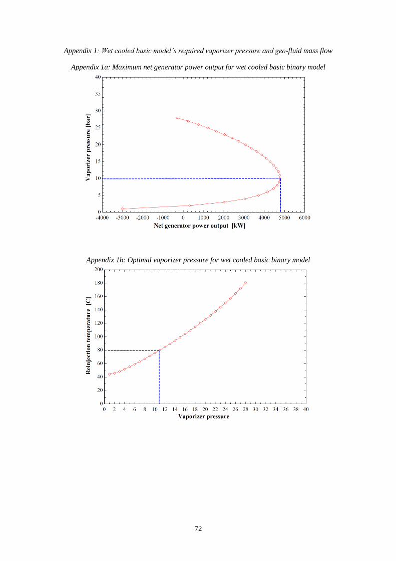
72
Appendix 1: Wet cooled basic model’s required vaporizer pressure and geo-fluid mass flow
Appendix 1a: Maximum net generator power output for wet cooled basic binary model
Appendix 1b: Optimal vaporizer pressure for wet cooled basic binary model
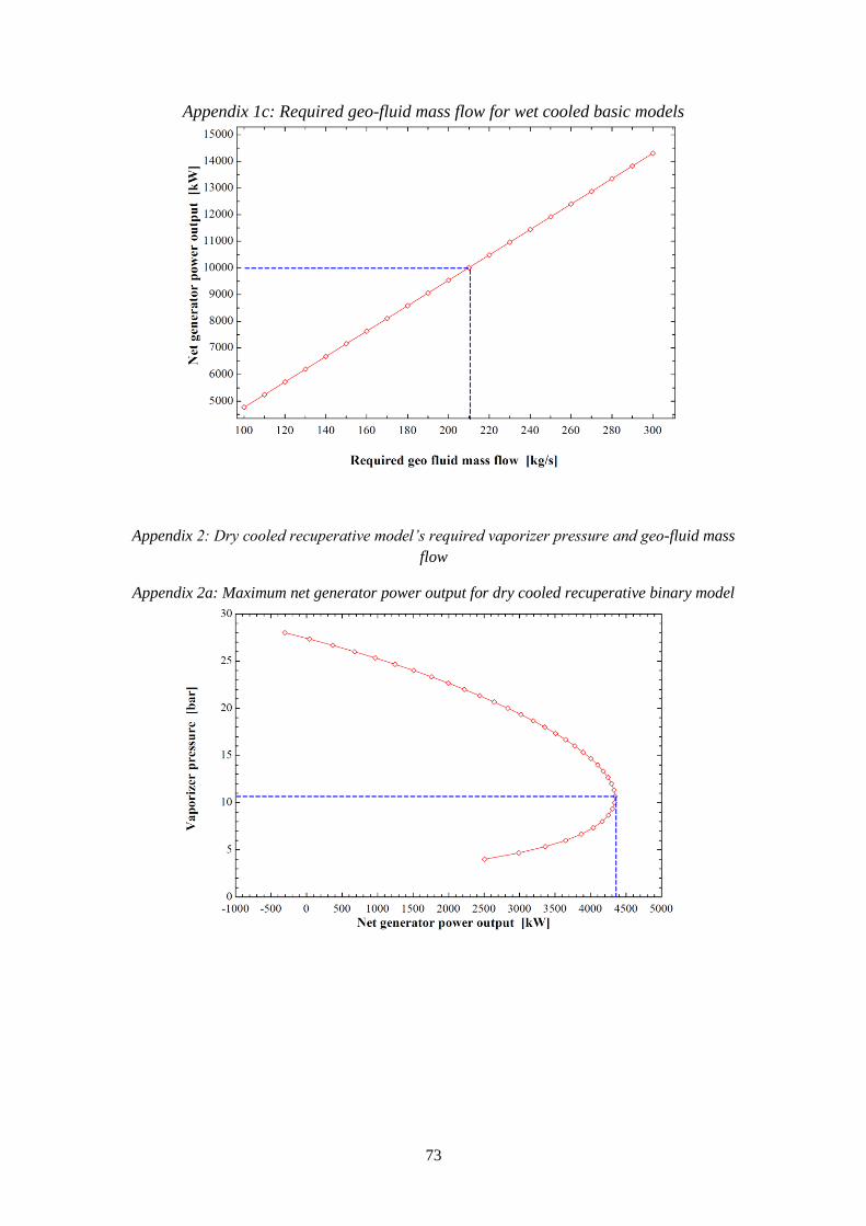
73
Appendix 1c: Required geo-fluid mass flow for wet cooled basic models
Appendix 2: Dry cooled recuperative model’s required vaporizer pressure and geo-fluid mass
flow
Appendix 2a: Maximum net generator power output for dry cooled recuperative binary model
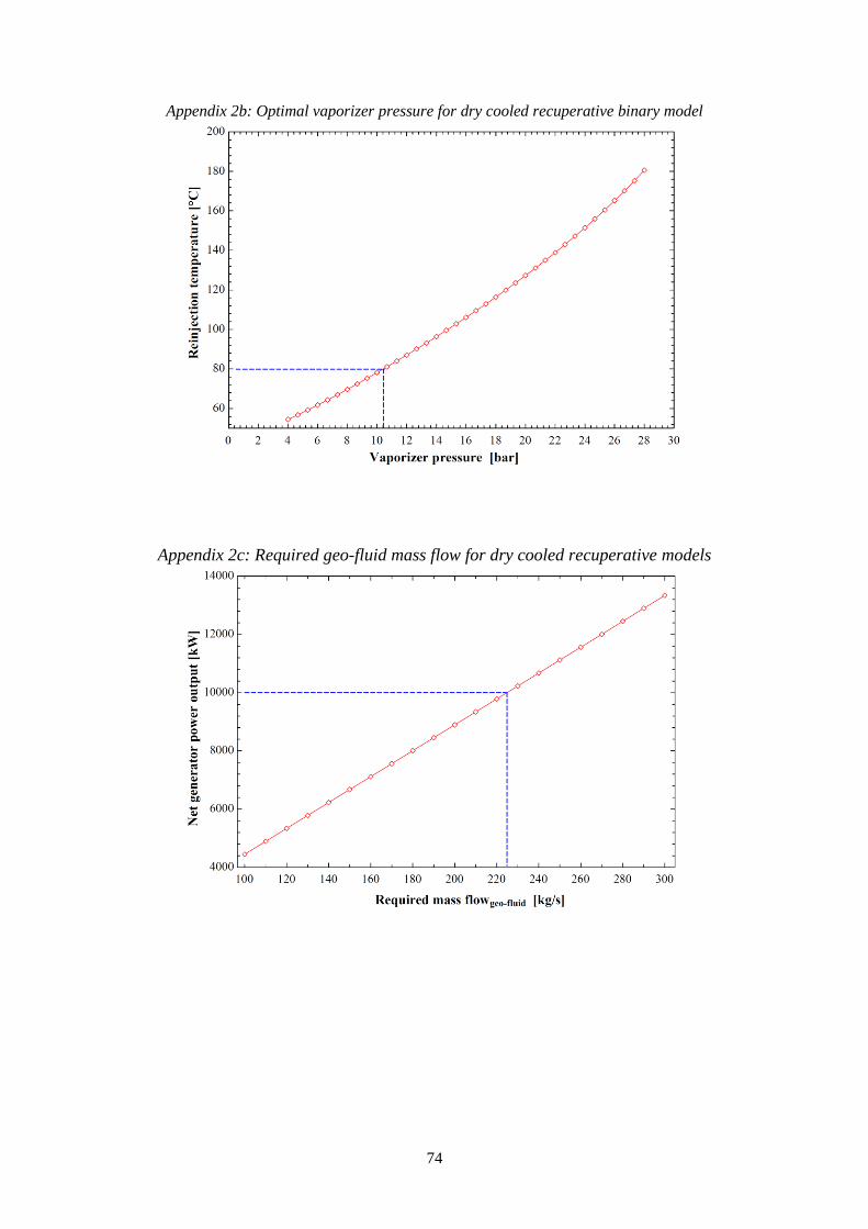
74
Appendix 2b: Optimal vaporizer pressure for dry cooled recuperative binary model
Appendix 2c: Required geo-fluid mass flow for dry cooled recuperative models
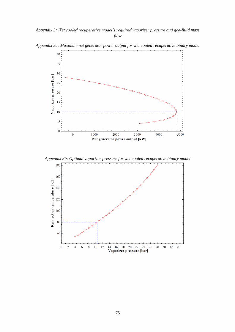
75
Appendix 3: Wet cooled recuperative model’s required vaporizer pressure and geo-fluid mass
flow
Appendix 3a: Maximum net generator power output for wet cooled recuperative binary model
Appendix 3b: Optimal vaporizer pressure for wet cooled recuperative binary model
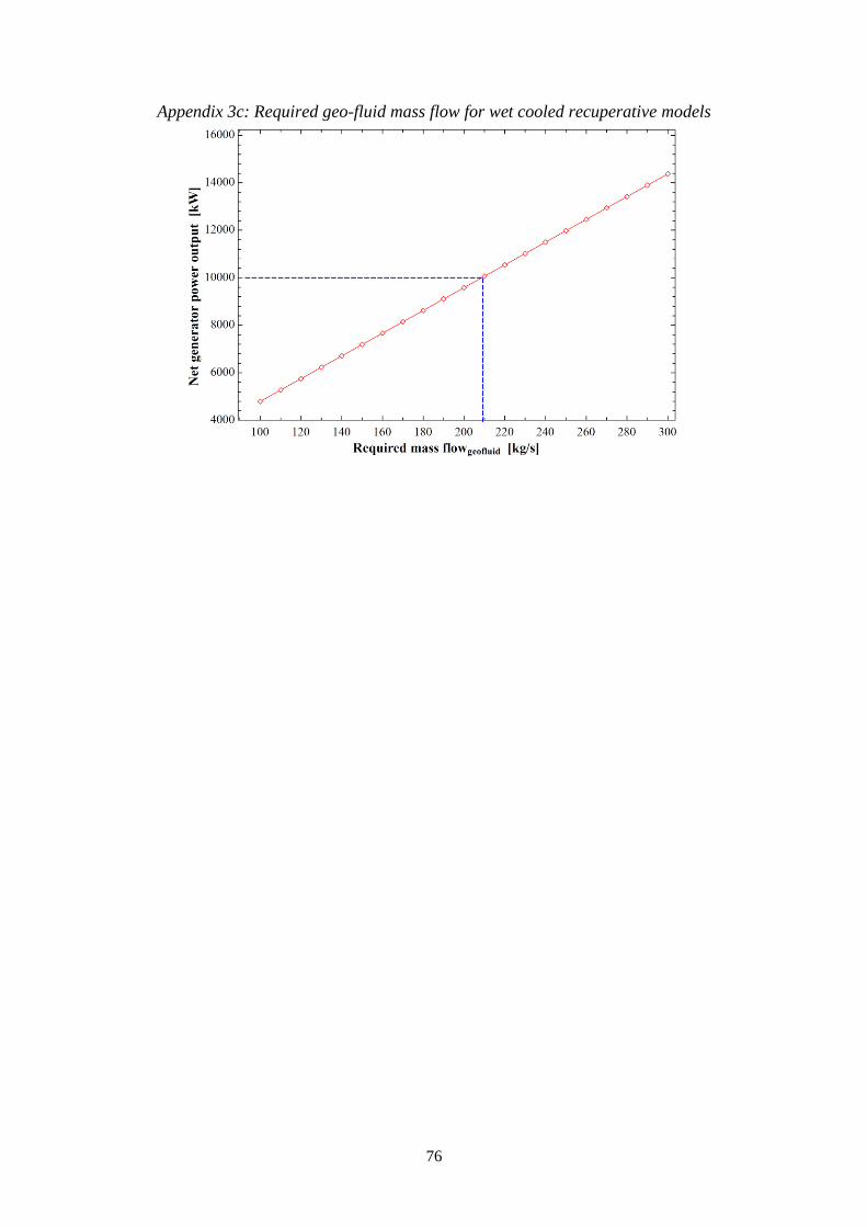
76
Appendix 3c: Required geo-fluid mass flow for wet cooled recuperative models
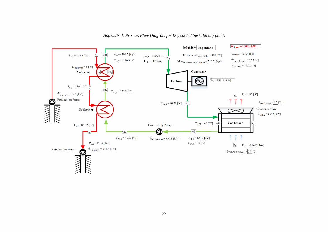
77
Appendix 4: Process Flow Diagram for Dry cooled basic binary plant.
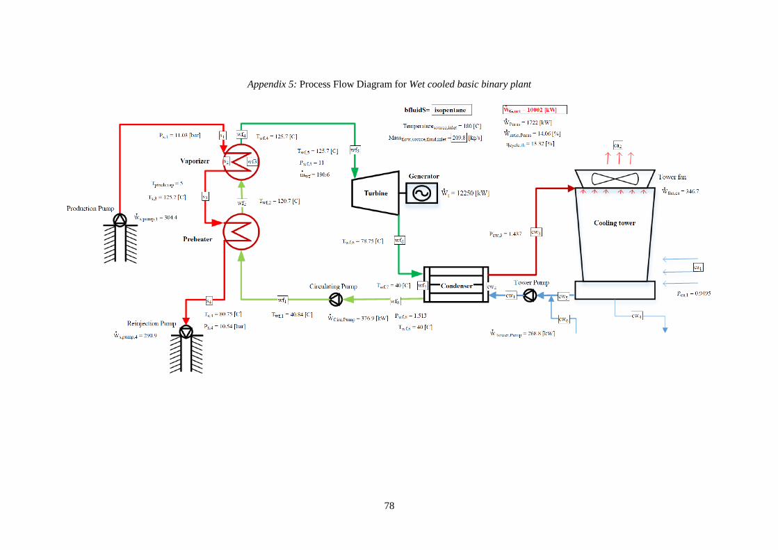
78
Appendix 5: Process Flow Diagram for Wet cooled basic binary plant
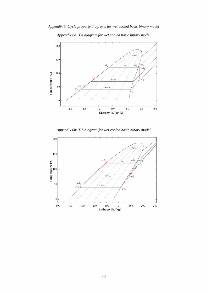
79
Appendix 6: Cycle property diagrams for wet cooled basic binary model
Appendix 6a: T-s diagram for wet cooled basic binary model
Appendix 6b: T-h diagram for wet cooled basic binary model
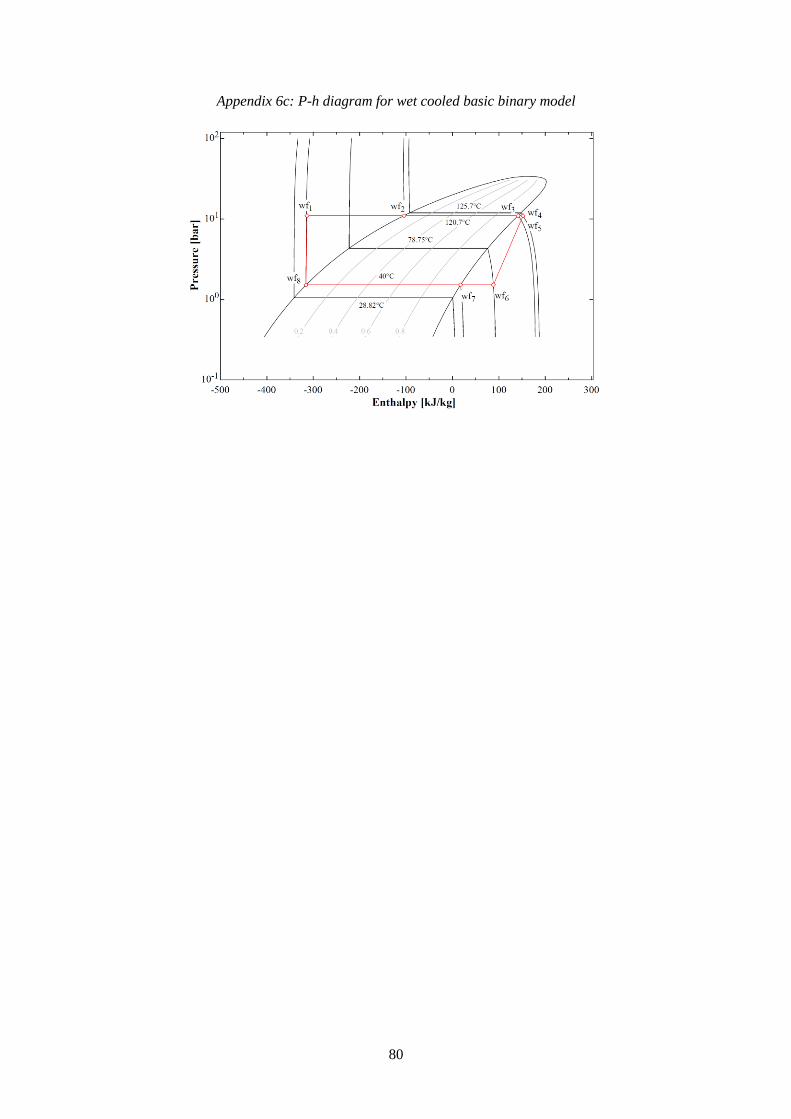
80
Appendix 6c: P-h diagram for wet cooled basic binary model
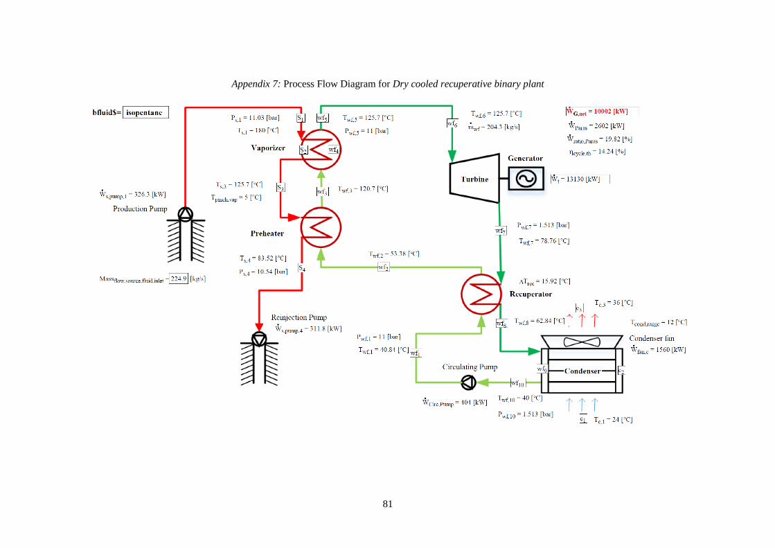
81
Appendix 7: Process Flow Diagram for Dry cooled recuperative binary plant
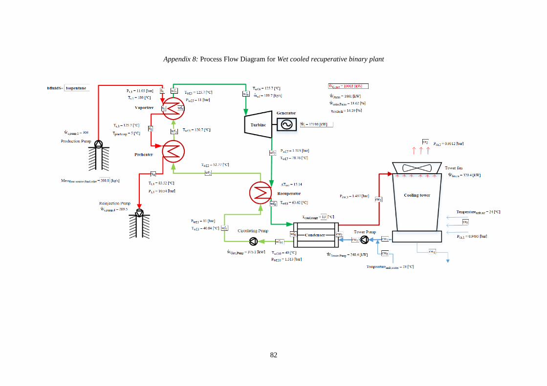
82
Appendix 8: Process Flow Diagram for Wet cooled recuperative binary plant
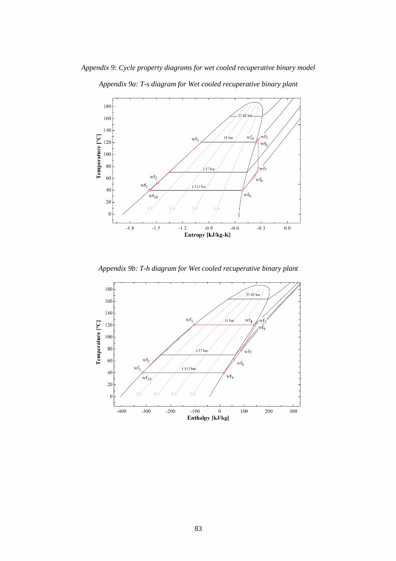
83
Appendix 9: Cycle property diagrams for wet cooled recuperative binary model
Appendix 9a: T-s diagram for Wet cooled recuperative binary plant
Appendix 9b: T-h diagram for Wet cooled recuperative binary plant
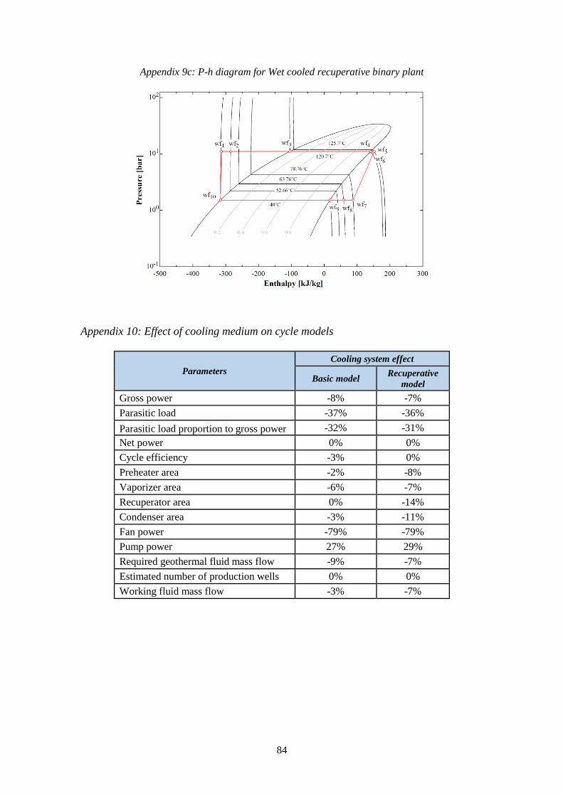
84
Appendix 9c: P-h diagram for Wet cooled recuperative binary plant
Appendix 10: Effect of cooling medium on cycle models
Parameters
Cooling system effect
Basic model Recuperative
model
Gross power -8% -7%
Parasitic load -37% -36%
Parasitic load proportion to gross power -32% -31%
Net power 0% 0%
Cycle efficiency -3% 0%
Preheater area -2% -8%
Vaporizer area -6% -7%
Recuperator area 0% -14%
Condenser area -3% -11%
Fan power -79% -79%
Pump power 27% 29%
Required geothermal fluid mass flow -9% -7%
Estimated number of production wells 0% 0%
Working fluid mass flow -3% -7%