PRESSURE PROGNOSIS AND MUD-WEIGHT DESIGN WHEN

DRILLING IN SALT ENVIRONMENTS

H. B. Helle1, J. M. Carcione2* and A. F. Gangi3

1. Nyborg Geoconsult, Bergen, Norway. hbhelle@broadpark.no 2. Istituto Nazionale di Oceanografia e di Geofisica Sperimentale (OGS), Trieste, Italy.

jcarcione@ogs.trieste.it *) corresponding author. 3. Department of Geology and Geophysics, Texas A&M University, College Station, Texas

77843-3114, USA. gangi@tamu.edu Keywords: formation pressure, mud-weight, rocksalt, drilling, stability, borehole

Resumen Las propiedades de la roca de sal para deformarse bajo la influencia de la temperatura y la tensión y su baja permeabilidad, hacen que las estructuras salinas sean una buena trampa de hidrocarburos y una roca sello ideal. Sin embargo, las formaciones salinas constituyen un riesgo en la perforación de un pozo de petróleo. A pesar del sistema de tensiones complejo debido a la combinación de los esfuerzos tectónicos y a fenómenos de compactación desequilibrada, demostramos en esta nota que se puede predecir la presión poral con datos sísmicos y de pozo en una mini-cuenca del Golfo de Méjico. Esto es posible usando un método clásico de mecánica de suelos y con la disponibilidad de datos suficientes de calibración. La roca de sal se comporta en formas diferentes a otras rocas, ya que puede fluir en tiempos relativamente cortos dependiendo de la las condiciones de tensión y temperatura. Esto puede producir deformaciones importantes del pozo con graves consecuencias para la perforación y el entubado. En esta nota, hemos desarrollado un método teórico para analizar la estabilidad antes y después de la perforación, y hemos obtenido ecuaciones de la forma y del area del pozo, del tiempo de colapso, y del peso del barro de perforación óptimo para evitar el colapso o la expansión de las paredes del pozo.

Abstract

The ability of salt to deform under temperature and stress, and its very low permeability make it a successful hydrocarbon-trap generator and an ideal seal, but a challenge for well design and drilling operations. Despite complex stress patterns due to combined action of salt tectonics and compaction disequilibrium, we demonstrate that accurate pressure prediction from seismic and well data in a Gulf of México mini-basin is feasible using a classical soil-mechanical approach provided sufficient calibration data are available. Rocksalt behaves differently from other rocks in that it has the ability to creep and flow significantly with time depending on the stress and temperature conditions, leading to borehole deformation that hampers the drilling and casing operations. We have developed a theoretical approach to analyze the stability during and after drilling, and we obtain expressions for the shape of the borehole cross section, the borehole-closure time and the optimal mud-weight to avoid wall collapse and expansion.

INTRODUCTION Exploration areas, where massive salt bodies are dominating features, constitute a challenge for well design and drilling operations. The ability of salt to deform under temperature and stress, and its very low permeability make it a successful hydrocarbon-trap generator and an ideal seal. The many possible types of hydrocarbon traps near the salt structures increase the potential of significant hydrocarbon accumulation. A common type of hydrocarbon trap, e.g. in Gulf of México (GoM), is that confined to the deformed sediments at the flanks of the salt domes where structural traps are created by the penetration of the buoyant salt body into the virgin sediment layering. Prospects where the reservoir seals are massive salt layers constitute the common plays in the Middle East as well as in deep-water GoM. In a young sedimentary basin such as Gulf of México, the combined action of salt tectonics and compaction disequilibrium may locally create complex stress patterns. Shear stresses adjacent to salt bodies may be highly amplified beyond the far-field values (Fredrich et al.,2003). Pressure prognosis and well design are thus challenging tasks. However, in areas of good seismic coverage with accurate velocity analysis these stress patterns are reasonable well expressed in the velocity cube and the seismic velocity field thus constitute an important support in the pre-drill pressure and well-stability analysis. A case history of pressure and wellbore stability analysis based on well and seismic data from GoM will be presented. To reach traps at the dome flanks the usual well trajectory is through the sediments and follows along the salt/sediment boundary. However, to reach target by penetrating the salt section is now gaining popularity as the industry gains experience and becomes aware of the several advantages of drilling through, rather than around the salt. Fracture gradients in shallow salt intervals have proven to be much higher than in non-salt sediments at a comparable depth. As a result of the increased fracture pressure, massive salt sections have been used to extend casing points and to eliminate casing strings, resulting in a greatly reduced well cost. Many operators are now choosing to drill massive salt sections to take the advantage of these benefits (Barker and Meeks, 2003). Drilling through shallow massive salt layers to reach deep sub-salt prospect is therefore feasible. For salt at greater depths, however, the elevated temperature becomes important for the shear strength of the material and thus for the stability of the well bore. The initial stress anisotropy then turns out to be a critical factor in design of drilling mud to prevent collapse or expansion of the borehole. A recent theory for borehole stability calculations by Carcione, Helle and Gangi (2005) will be briefly reviewed. In this paper we first shortly review the concepts of geopressure and then discuss abnormal pressure due non-equilibrium compaction and its effect on seismic attributes. A review of the rock physics of geopressure is given in a recent study by Carcione and Helle (2002). Next, we present the methods and associated formula applied in this project, based on the “best practice” procedures for deepwater GoM summarized in Knowledge System (2001), followed by a presentation of the data analysis and results of pressure prediction in the GoM well.

Geopresssure Abnormal pressure, or pressures above or below hydrostatic pressure, occurs on all continents in a wide range of geological conditions. Various physical processes cause anomalous pressures in an underground fluid. The most commonly cited mechanisms for abnormal pressure generation in petroleum provinces are compaction disequilibrium and hydrocarbon generation including oil-to-gas cracking (Mann and Mackenzie, 1990; Luo and Vasseur, 1994; Berg and Gangi, 1999). In young (Tertiary) deltaic sequences, compaction disequilibrium is the dominant cause of abnormal pressure. In older (pre-Tertiary) lithified rocks, hydrocarbon generation and tectonics are most often cited as the causes of overpressure (Law et al, 1998). Hydrocarbon accumulations are frequently found in close association with abnormal pressure. In exploration for hydrocarbons and exploitation of the reserves, knowledge of the pressure distribution is of vital importance for prediction of the reserves, for the safety of the drilling and for optimising the recovery rate. Moreover, drilling of deep gas resources is hampered by high risk associated with unexpected overpressure zones. Knowledge of pore pressure using seismic data, such as for instance seismic-while-drilling

techniques, will help producers plan the drilling process in real-time to control potentially dangerous abnormal pressures.

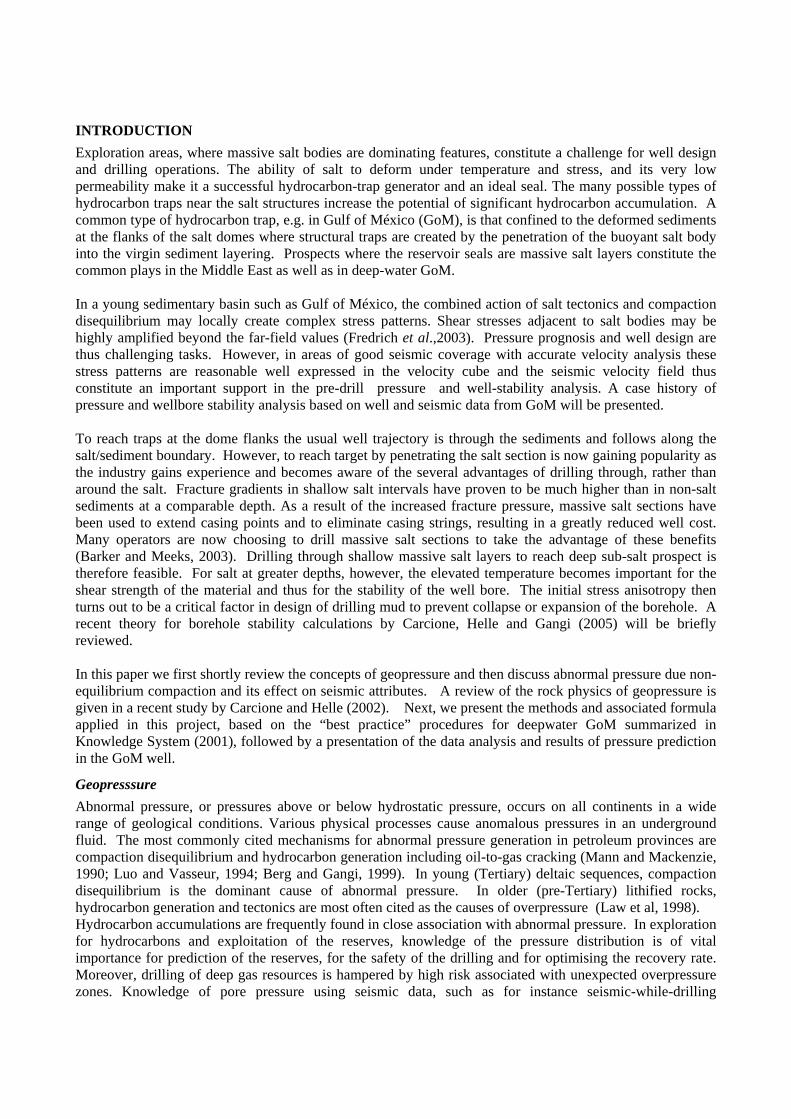
In order to illustrate the physics of geopressure, let us review the main concepts (see Figure 1). Pore pressure, also known as formation pressure, is the in situ pressure of the fluids in the pores. The pore pressure is equal to the hydrostatic pressure when the pore fluids support only the weight of the overlying pore fluids (mainly brine). The lithostatic or confining pressure is due to the weight of overlying sediments, including the pore fluids. In the absence of any state of stress in the rock, the pore pressure attains lithostatic pressure and the fluids support all the weight. However, fractures perpendicular to the minimum compressive stress direction appear for a given pore pressure, typically 70-90% of the confining pressure. In this case, the fluid escapes from the pores and pore pressure decreases. A rock is said to be overpressured when its pore pressure is significantly greater than hydrostatic pressure. The difference between confining pressure and pore pressure is called differential pressure. In the context of well planning and drilling, the objective is to estimate in advance the mudpressure, or equivalent density of the drilling fluid (EMW) required to balance the formation pressure but to avoid fracturing. For high overpressure or low formation strength, the mudpressure window may be quite narrow and with the resulting high risk for well flow (kicks) and losses.

MMWW

ppffrr

Figure 1: Typical pressure vs. depth plot where the different pressure definitions are illustrated. The objective is to determine a mudpressure (MW) between pore pressure and fracturing pressure frp .

In deeply buried oil reservoirs, oil-to-gas cracking may

increase the pore pressure so that it reaches or exceeds the lithostatic pressure (Chaney, 1950; Barker, 1990; Luo and Vasseur, 1996; Berg and Gangi, 1999). Oil can be generated from kerogen-rich source rocks and flow through a carrier bed to a sandstone reservoir rock. Excess pore-fluid pressures in sandstone reservoirs are generated when the rate of volume created by the transformation of oil to gas is more rapid than the rate of volume loss by fluid flow. If the reservoir is sealed on all sides by an impermeable shale or limestone, then the condition of a closed system will be satisfied for gas generation. Due to the presence of semi-vertical fault planes and compartmentalization, this condition holds for most North Sea reservoirs. Non-equilibrium compaction or mechanical compaction disequilibrium is a consequence of a rapid deposition compared with the rate of expulsion of pore fluids by gravitational compaction. In this situation, the fluids carry part of the load that would be held by grain contacts and abnormal pore pressures develop in the pore-space. A description of this overpressure mechanism is given by Rubey and Hubbert (1959) and mathematical treatments of the problem are provided, for instance, by Bredehoeft and Hanshaw (1968), and Smith (1971) and Dutta (1983). These models use Darcy's law and their predictions are greatly affected by the choice of the constitutive relations between porosity, permeability and effective stress.

Abnormal pressure due to disequilibrium compaction. The sediments in Gulf of México at prospective depths are of Tertiary origin, with an age of less than 10 My. The area is characterized by high sedimentation rates implying weak consolidation and soft rock material compared with those of prospective levels in the North Sea. Young sediments and high sedimentation rates imply that the classical soil-mechanical principles such as Terzaghi’s model (Terzaghi and Peck, 1948) and its derivatives (Eaton, 1976; Bowers, 1995; Baldwin and Butler, 1985) may apply. In a recent study (Knowledge System, 2001) under the auspices of the Drilling Engineering Association (DEA) the best practice procedures for predicting geopressure in deep water GoM have been evaluated and ranked according to their accuracy when applied to a number of test wells (>100) in the area. In this study we have essentially exploited the recipes provided in the DEA report.

The case of non-equilibrium compaction is that in which the sedimentation rate is so rapid that the pore fluids do not have a chance to 'escape'. We assume that the pore-space is filled with organic material and water, that the compressibilities of the organics and water are independent of pressure and temperature, and that of the rock is independent of temperature but depends on pressure. At time , corresponding to depth

, with initial hydrostatic fluid pressure it

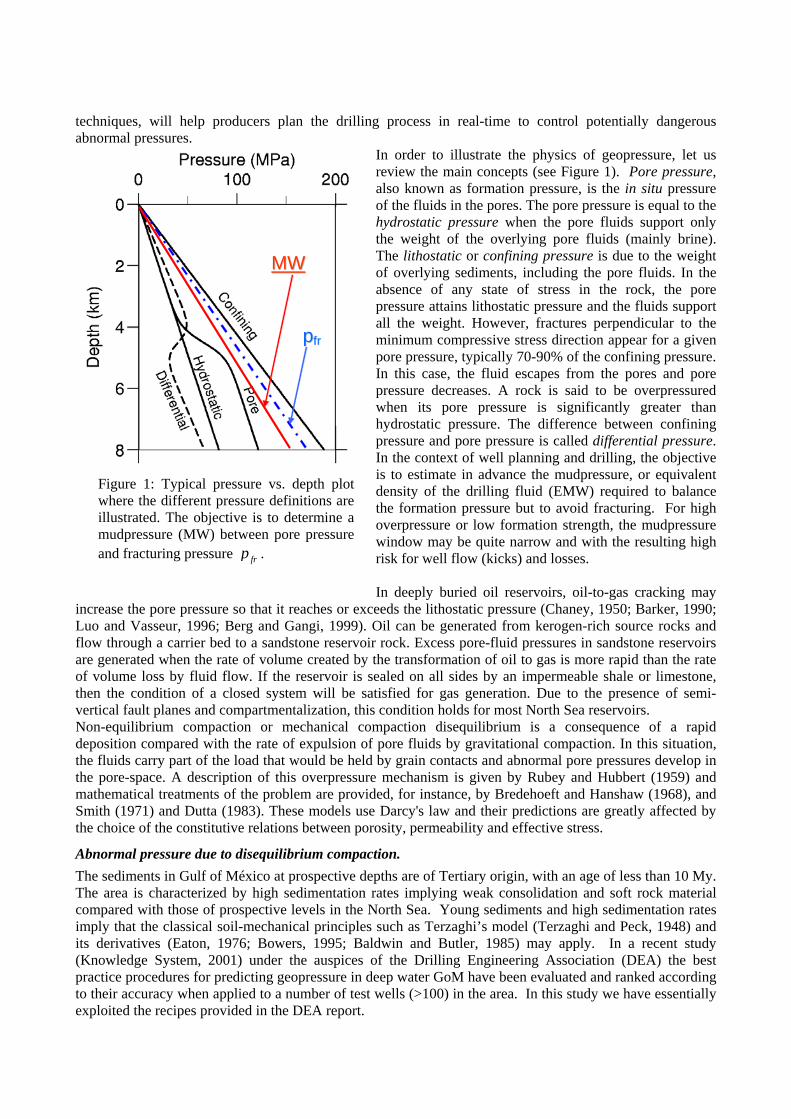
iz i wp g izρ= , the volume of rock behaves as a closed system. That is, if the unit is shale, its permeability is extremely low, and if the unit is sandstone, the permeability of the sealing faults is sufficiently low so that the rate of pressure increase greatly exceeds the dissipation of pressure by flow. Pore pressure excess is measured relative to hydrostatic pressure. The pore-pressure buildup with depth for different pore fluids is shown in Figure 2, where the continuous lines represent the hydrostatic and lithostatic pressures. The dotted line corresponds to full light-oil saturation, and the broken lines to full Winkler's oil saturation (label 1), partial saturation (Swi = 0.5 and heavy oil) (label 2), and full heavy-oil saturation (label 3). As can be appreciated, the rock is underpressured for full light-oil saturation and increasing pore-fluid bulk modulus gives overpressure. For low compressibilities and high thermal expansion coefficients of the pore fluid, the pore pressure may exceed the lithostatic pressure. In the case of heavy oil, the cause is the high thermal expansion coefficient. Non-equilibrium compaction generates abnormal fluid pressures that, under certain conditions, can be detected with seismic methods. This is very important in drilling applications. The results for a model in which a reservoir volume is buried at a constant sedimentation rate, with a geothermal gradient which is constant both in time and depth, show that wave velocities and quality factors decrease with decreasing differential

pressure (or effective pressure). The large change is mainly due to the fact that the dry-rock moduli are functions of the effective pressure, with the largest changes occurring at low differential pressures. For a given pore-space compressibility, the fluid mixture filling the pore-space has a major influence on P-wave velocity and may cause underpressure or overpressure depending on its compressibility and thermal expansion coefficient. Rocks saturated with fluids of high compressibility and low thermal expansion coefficient are generally underpressured, and rocks saturated with fluids of low compressibility and high thermal expansion coefficient are generally overpressured, and can be seismically "visible". At high differential pressures the velocities are almost constant. Perceptible changes in the velocities occur when the differential pressure decreases to 20 MPa and become significant when the differential pressure decreases to about 15 MPa. The quality factor curve for full water saturation calculated with the present model is in good agreement with experimental values obtained in the ultrasonic frequency band. The model is able to predict pore pressure from seismic properties if reliable estimates of wave velocities and quality factors can be obtained.

Figure 2: Pore-pressure build-up with depth for different pore fluids, where the continuous lines represent the hydrostatic and lithostatic pressures. The dotted line corresponds to full light-oil saturation, and the broken lines to full heavy-oil saturation (label 1), partial saturation (Swi=0.5 and heavy oil) (label 2), and full heavy oil saturation (label 3).

ESTIMATION OF GEOPRESSURE FROM SEISMIC AND WELL DATA. A PRACTICAL APPROACH TO A GULF OF MÉXICO PROSPECT.

Let us assume a rock at depth z. The lithostatic or confining pressure can be obtained by integrating the density log. We have that

cp

0

( )z

cp g z dρ= ∫ z , (1)

where ρ is the density and g is the acceleration of gravity. The bulk density is given by ( ) (1 )f gzρ φρ φ ρ= + − , (2)

where and g fρ ρ are the density of the grain material and pore fluid, respectively, and the porosity φ can be obtained from the density log by the relationship

g

g fρ

ρ ρφ

ρ ρ−

=−

, (3)

or from the sonic log by the relationship

ft

f g

t tt t

φ∆

∆ − ∆=

∆ − ∆, (4)

where are the transit times of the grain material, fluid and the bulk, respectively. , and∆ ∆ ∆g ft t t

A more practical equation (Schlumberger, 1989) for fitting to experimental data is

gt

t tC

tφ∆

∆ − ∆′ =

∆, (5)

where 60 s/ftgt µ∆ ≈ is the transit time for the grain material and a fit to experimental data can made by varying C only. Published values of C are in the range 0.6-1.0 (Schlumberger, 1989).

In this example, we have exploited the density log in the calibration well and equation (3) to calibrate (5) to obtain a consistent estimate of φ from seismic velocity and the sonic logs. Furthermore, the hydrostatic pressure is given by

0

( )z

f fp g z dz g f zρ ρ= ≈∫ , (6)

where density of the fluid (brine) is set to 31030 kg/mfρ = and acceleration due to gravity g = 9.81 m/s2.

Formation Pressure There are several means of estimating the formation pressure from velocity. All the methods require regional and local calibration but, fortunately, a ranking list of empirical equations for deep water GoM is provided by the recent DEA report (Knowledge System, 2001) where the Baldwin-Butler type porosity-effective stress formulation

, (7) 1.0945635(1 )C Amop p φ= − − co

with 1.425(1 /15000)Amoco PVφ = − (8)

has been given highest rank based on accuracy when tested in more than 100 deep-water wells. Here, the units for pressure are pounds per square inch (psi), and for the velocity the unit is feet per second (ft/s). PV Fracturing pressure Also according to a ranking list in the DEA report (Bowers, 2001) the minimum stress method is the preferred approach for predicting fracture gradient. All minimum stress methods are based on the equation (Hubbert and Willis, 1957)

( )fr Cp K p p= − + p , (9)

where K is the effective stress ratio (also termed matrix stress coefficient) set to by Hubbert and Willis (1957) but allowed to vary with depth, in the range 0.3-1.0, by Pennebaker (1968), from values of about 0.3 for shallow layers to values near 1.0 at depths. To account for the variation of

1/ 3K =

K with depth we introduce the function

0 01 (1 ) exp[ ( )]K K z zγ= − − − − , (10)

where is the depth of the mudline (where 0z 0 0.3K K= ≈ ) and 0K and γ can be determined by fit to regional LOT data (or data provided by Pennebaker, 1968).

AB

Sal

t D

iap

er

0 2 4 6 8 km

6

5

4

3

2

Dep

th (k

m)

ABS

alt

Dia

per

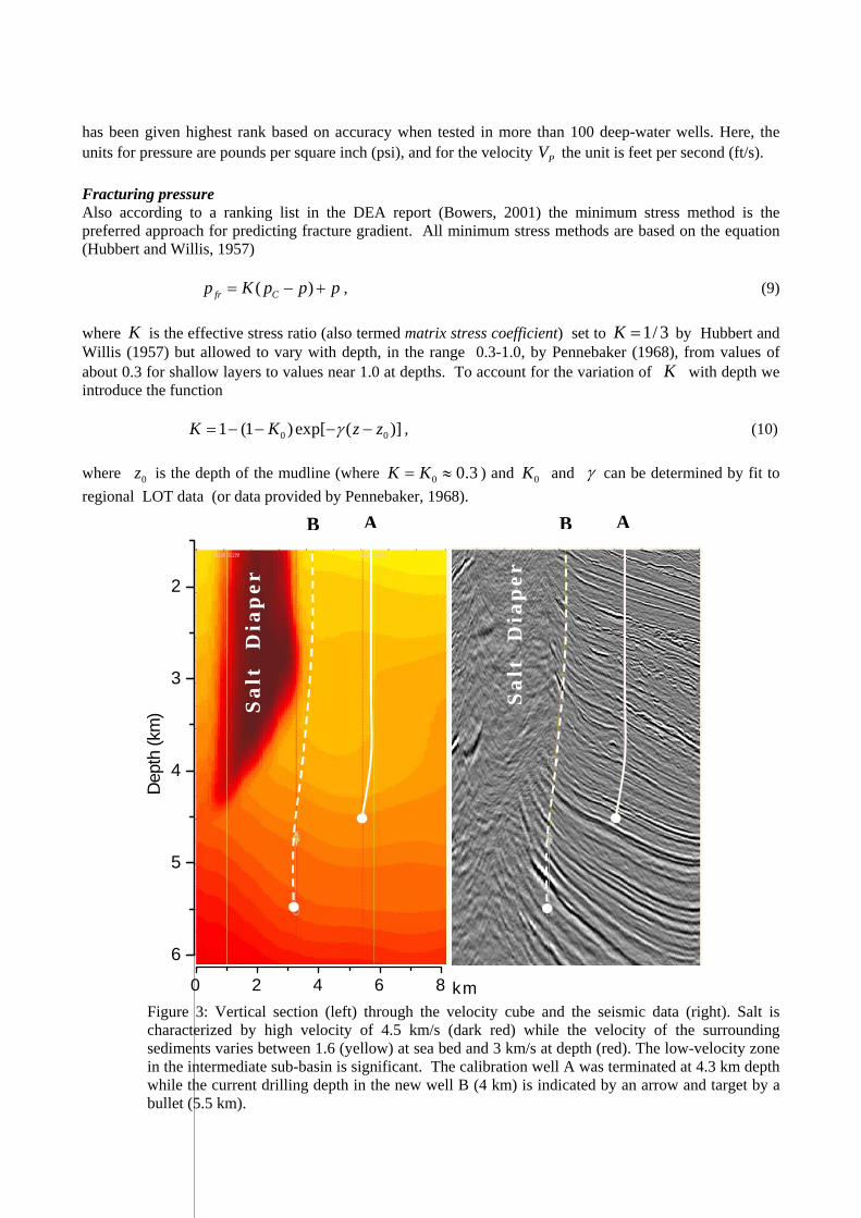
Figure 3: Vertical section (left) through the velocity cube and the seismic data (right). Salt is characterized by high velocity of 4.5 km/s (dark red) while the velocity of the surrounding sediments varies between 1.6 (yellow) at sea bed and 3 km/s at depth (red). The low-velocity zone in the intermediate sub-basin is significant. The calibration well A was terminated at 4.3 km depth while the current drilling depth in the new well B (4 km) is indicated by an arrow and target by a bullet (5.5 km).

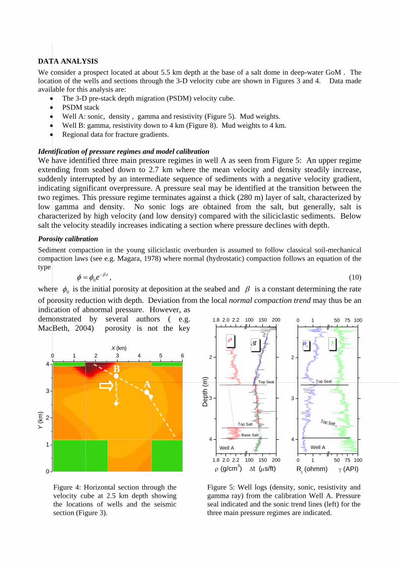
DATA ANALYSIS We consider a prospect located at about 5.5 km depth at the base of a salt dome in deep-water GoM . The location of the wells and sections through the 3-D velocity cube are shown in Figures 3 and 4. Data made available for this analysis are:

• The 3-D pre-stack depth migration (PSDM) velocity cube. • PSDM stack • Well A: sonic, density , gamma and resistivity (Figure 5). Mud weights. • Well B: gamma, resistivity down to 4 km (Figure 8). Mud weights to 4 km. • Regional data for fracture gradients.

Identification of pressure regimes and model calibration We have identified three main pressure regimes in well A as seen from Figure 5: An upper regime extending from seabed down to 2.7 km where the mean velocity and density steadily increase, suddenly interrupted by an intermediate sequence of sediments with a negative velocity gradient, indicating significant overpressure. A pressure seal may be identified at the transition between the two regimes. This pressure regime terminates against a thick (280 m) layer of salt, characterized by low gamma and density. No sonic logs are obtained from the salt, but generally, salt is characterized by high velocity (and low density) compared with the siliciclastic sediments. Below salt the velocity steadily increases indicating a section where pressure declines with depth.

Porosity calibration Sediment compaction in the young siliciclastic overburden is assumed to follow classical soil-mechanical compaction laws (see e.g. Magara, 1978) where normal (hydrostatic) compaction follows an equation of the type

0ze βφ φ −= , (10)

where 0φ is the initial porosity at deposition at the seabed and β is a constant determining the rate of porosity reduction with depth. Deviation fromindication of abnormal pressure. However, as demonstrated by several authors ( e.g. MacBeth, 2004) porosity is not the key

0

1

2

3

4

Y (k

m)

0 1 2 3 4 5

the local normal compaction trend may thus be an

6 X (km)

BA

4

3

2

1.8 2.0 2.2 100 150 200

1.8 2.0 2.2 100 150 200

Well A

Base Salt

Top Salt

Top Seal

∆t ρ

ρ (g/cm3) ∆t (µs/ft)

Dep

th (m

)

4

3

2

0 1 50 75 100

0 1 50 75 100

Well A

Top Seal

Top Salt

γ Rt

Rt (ohmm) γ (API)

Figure 5: Well logs (density, sonic, resistivity and gamma ray) from the calibration Well A. Pressure seal indicated and the sonic trend lines (left) for the three main pressure regimes are indicated.

Figure 4: Horizontal section through the velocity cube at 2.5 km depth showing the locations of wells and the seismic section (Figure 3).

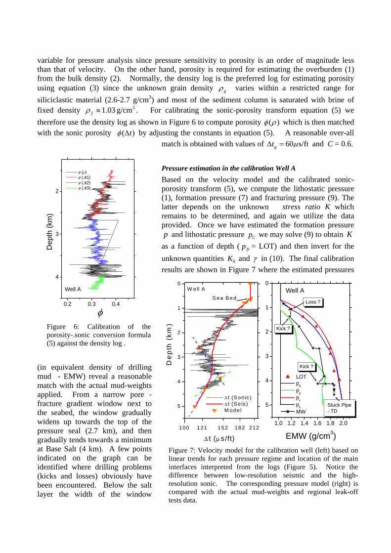
variable for pressure analysis since pressure sensitivity to porosity is an order of magnitude less than that of velocity. On the other hand, porosity is required for estimating the overburden (1) from the bulk density (2). Normally, the density log is the preferred log for estimating porosity using equation (3) since the unknown grain density gρ varies within a restricted range siliciclastic material (2.6-2.7 g/cm3) and most of the sediment column is saturated with brine of fixed density 31.03 g/cmfρ ≈ . For calibrating the sonic-porosity transform equation (5) we therefore use the density log as shown in Figure 6 to compute porosity ( )

for

φ ρ which is then matched the sonic porosity ( )twith φ ∆ by adjusting the consta equation (5). A reasonable over-all

match is obtained with values of 60 s/ftgtnts in

µ∆ = and C = 0.6.

re estimation in the calibration calibrated sonic-

Pressu Well A Based on the velocity model and the porosity transform (5), we compute the lithostatic pressure (1), formation pressure (7) and fracturing pressure (9). The latter depends on the unknown stress ratio K which remains to be determined, and again we utilize the data provided. Once we have estimated the formation pressure p and lithostatic pressure Cp we may solve (9) to obtain K

a function of depth (as frp LOT) and then invert for t unknown quantities

= he

0K a nd γ in (10). The final calibration results are shown in gure 7 where the estimated pressures

(in equivalent density of drilling mud - EMW) reveal a reasonable match with the actual mud-weights applied. From a narrow pore - fracture gradient window next to the seabed, the window gradually widens up towards the top of the pressure seal (2.7 km), and then gradually tends towards a minimum at Base Salt (4 km). A few points indicated on the graph can be identified where drilling problems (kicks and losses) obviously have been encountered. Below the salt layer the width of the window

Fi

5

4

3

2

1

0

100 121 152 182 212

S ea B ed

W ell A

∆ t (µs/ft)

De

pth

(km

)

∆ t (S on ic) ∆ t (S e is ) M ode l

5

4

3

2

1

1.0 1.2 1.4 1.6 1.8 2.0

0

Stuck Pipe- TD

Kick ?

Kick ?

Loss ?

Well A

EMW (g/cm3)

LOT pfr pp pc ph MW

4

3

2

0.2 0.3 0.4

Well A

Dep

th (k

m)

φ

φ (ρ) φ (∆t1) φ (∆t2) φ (∆t3)

Figure 6: Calibration of the porosity-.sonic conversion formula (5) against the density log .

Figure 7: Velocity model for the calibration well (left) based on linear trends for each pressure regime and location of the main interfaces interpreted from the logs (Figure 5). Notice the difference between low-resolution seismic and the high-resolution sonic. The corresponding pressure model (right) is compared with the actual mud-weights and regional leak-off tests data.

gradually increases with depth, indication that safe drilling below salt should be feasible. However, due to stuck pipe the well was terminated before reaching the target, probably caused by hole instability (creep) in the salt section.

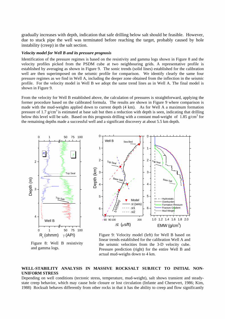
Velocity model for Well B and its pressure prognosis Identification of the pressure regimes is based on the resistivity and gamma logs shown in Figure 8 and the velocity profiles picked from the PSDM cube at two neighbouring grids. A representative profile is established by averaging as shown in Figure 9. The sonic trends (solid lines) established for the calibration well are then superimposed on the seismic profile for comparison. We identify clearly the same four pressure regimes as we find in Well A, including the deeper zone obtained from the inflection in the seismic profile. For the velocity model in Well B we adopt the same trend lines as in Well A. The final model is shown in Figure 9. From the velocity for Well B established above, the calculation of pressures is straightforward, applying the former procedure based on the calibrated formula. The results are shown in Figure 9 where comparison is made with the mud-weights applied down to current depth (4 km). As for Well A a maximum formation pressure of 1.7 g/cm3 is estimated at base salt but then a reduction with depth is seen, indicating that drilling below this level will be safe. Based on this prognosis drilling with a constant mud-weight of 1.85 g/cm3 for the remaining depths made a successful well and a significant discovery at about 5.5 km depth.

4

3

2

0 1 50 75 100

0 1 50 75 100

Well B

Top Salt

Top Seal

γ Rt

Rt (ohmm) γ (API)

Dep

th (m

)

6

5

4

3

2

1

0

80 90100 200

Well B

1/V(

Seis

)

Sea Bed

Base Salt

Top Seal

∆t (µs/ft)

Dep

th (k

m)

Model ∆t (seis) ∆t1 ∆t2

6

5

4

3

2

1

0

1.0 1.2 1.4 1.6 1.8 2.0

Base Salt

Top Seal

EMW (g/cm3)

Hydrostatic Overburden Formation Pressure Fracture Gradient Mud Weight

Figure 9: Velocity model (left) for Well B based on linear trends established for the calibration Well A and the seismic velocities from the 3-D velocity cube. Pressure prediction (right) for the entire Well B and actual mud-weighs down to 4 km.

Figure 8: Well B resistivity and gamma logs.

WELL-STABILITY ANALYSIS IN MASSIVE ROCKSALT SUBJECT TO INITIAL NON-UNIFORM STRESS Depending on well conditions (tectonic stress, temperature, mud-weight), salt shows transient and steady-state creep behavior, which may cause hole closure or lost circulation (Infante and Chenevert, 1986; Kim, 1988) Rocksalt behaves differently from other rocks in that it has the ability to creep and flow significantly

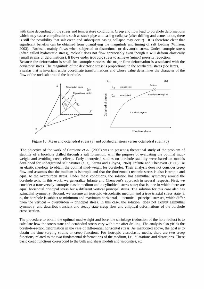
with time depending on the stress and temperature conditions. Creep and flow lead to borehole deformations which may cause complications such as stuck pipe and casing collapse (after drilling and cementation, there is still the possibility that salt creep and subsequent casing collapse may occur). It is therefore clear that significant benefits can be obtained from quantifying the magnitude and timing of salt loading (Willson, 2003). Rocksalt mainly flows when subjected to distortional or deviatoric stress. Under isotropic stress (often called hydrostatic stress), rocksalt does not flow appreciably even though it will deform elastically (small strains or deformations). It flows under isotropic stress to achieve (minor) porosity reduction. Because the deformation is small for isotropic stresses, the major flow deformation is associated with the deviatoric stress. The magnitude of the deviatoric stress is proportional to the octahedral stress (see later), a scalar that is invariant under coordinate transformations and whose value determines the character of the flow of the rocksalt around the borehole.

Figure 10: Mean and octahedral stress (a) and octahedral stress versus octahedral strain (b) The objective of the work of Carcione et al. (2005) was to present a theoretical study of the problem of stability of a borehole drilled through a salt formation, with the purpose of evaluating the optimal mud-weight and avoiding creep effects. Early theoretical studies on borehole stability were based on models developed for underground salt cavities (e. g., Serata and Gloyna, 1960). Infante and Chenevert (1986) use an elastic rheology to obtain the optimal mud-weight for boreholes. Their analysis does not consider creep flow and assumes that the medium is isotropic and that the (horizontal) tectonic stress is also isotropic and equal to the overburden stress. Under these conditions, the solution has azimuthal symmetry around the borehole axis. In this work, we generalize Infante and Chenevert's approach in several respects. First, we consider a transversely isotropic elastic medium and a cylindrical stress state; that is, one in which there are equal horizontal principal stress but a different vertical principal stress. The solution for this case also has azimuthal symmetry. Second, we assume an isotropic viscoelastic medium and a true triaxial stress state, i. e., the borehole is subject to minimum and maximum horizontal -- tectonic -- principal stresses, which differ from the vertical -- overburden -- principal stress. In this case, the solution does not exhibit azimuthal symmetry, and describes transient and steady-state creep flow and elliptical deformations of the borehole cross-section. The procedure to obtain the optimal mud-weight and borehole shrinkage (reduction of the hole radius) is to calculate how the stress state and octahedral stress vary with time after drilling. The analysis also yields the borehole-section deformation in the case of differential horizontal stress. As mentioned above, the goal is to obtain the time-varying strains or creep functions. For isotropic viscoelastic media, there are two creep functions, related to the two fundamental deformations of the medium, i.e., dilatations and distortions. These basic creep functions correspond to the bulk and shear moduli and viscosities, etc.

Mean, octahedral stresses and optimal mud pressure. Before drilling, the mean and octahedral stresses (Figure 10) are given by the equation

1 (3m H h )vσ σ σ σ= + + , (11)

and

2 22 33 2 2

H h H ho v

σ σ σ στ σ+ −⎛ ⎞ ⎛= − +⎜ ⎟ ⎜⎝ ⎠ ⎝

⎞⎟⎠

, (12)

where Hσ and hσ are the maximum and minimum horizontal stress components, respectively, and vσ is the vertical stress (overburden). After drilling a cylindrical borehole of radius 0r r= , the stress components in a cylindrical coordinate system at the borehole wall are given by

,( ) 2( )cos 2 ,0,

2 ( ) cos 2 ,

rr

H h H h

r

zz v H h

ppθθ

θ

σσ σ σ σ σ θσσ σ ν σ σ θ

= −= + − − +

== − −

(13)

where is the mud pressure, p ν is the Poisson ratio and θ is the polar angle in the horizontal plane with

0θ = in the direction of minimum horizontal stress. Let us calculate the optimal mud-weights or optimal borehole pressures to avoid borehole closure. The maximum stress concentration at the borehole wall occurs at / 2θ π= , where the above equations become

,3 ,0,

2 ( ).

rr

H h

r

zz v H h

ppθθ

θ

σσ σ σσσ σ ν σ σ

= −= − +

== + −

(14)

Using the definition of oτ in cylindrical coordinates we obtain from (14) the following relation:

2 2 29 6 6(3 ) 2(3 ) 2(3 ) 0o H h H h zz H hp pτ σ σ σ σ σ σ σ σ− + + − + − − + − =zz

2p

, (15) which solved for gives the following condition for the borehole pressure: p

1p p≤ − ≤ , (16) where

2 2 21

3 1 54 3(3 ) 12 12(3 ) ,2 6

H ho H h zz H hp zz

σ σ τ σ σ σ σ σ σ−= − − − − + − (17)

and 2 2 2

23 1 54 3(3 ) 12 12(3 ) .

2 6H h

o H h zz H hp zzσ σ τ σ σ σ σ σ σ−

= + − − − + − (18)

The maximum octahedral stress oτ should be less than oeτ , the octahedral-stress limit for elastic (unrelaxed) behavior, or less than the octahedral-stress limit for relaxed (plastic) behavior (see Figure 10). Steady-state creep effects in isotropic rock Viscoelastic flow (creep) is present at all levels of octahedral stress, but becomes important when oτ exceeds the elastic octahedral stress oeτ . Therefore, we assume that below this level we only have transient creep. For o oeτ τ> , where oτ is the maximum octahedral stress obtained from equation (15) we use the Maxwell model (Ben-Menahem and Singh, 1981; Klausner, 1991; Carcione, 2001) to describe the deformation of the borehole. Solving for the minor and major semiaxes of the elliptical crossection as a function of time we find:

0 2 2

0 2 2

1 1( ) 1 ( 2 ) ( ) ( )( 6 ( )) ,4 41 1( ) 1 ( 2 ) ( ) ( )( 6 ( )) ,4 4

H h H h

H h H h

a t r p t t

b t r p t t

σ σ χ σ σ χ χ

σ σ χ σ σ χ χ

⎡ ⎤= − + + − − +⎢ ⎥⎣ ⎦⎡ ⎤= − + + + − +⎢ ⎥⎣ ⎦

(19)

where the creep function is given by

21( ) 1 ( ),tt H t µη

χ τµ τ µ∞ ∞

⎛ ⎞= + =⎜ ⎟⎝ ⎠

, (20)

with µ∞ the relaxed ( t ) shear modulus and = ∞ µη the shear viscosity of the material, and ( )H t is the Heavyside function. The second creep function is given by

[ ]11

1 1( ) 1 exp( ( )3

ttk b

χµ η∞ ∞

⎧ ⎫= + + − −⎨ +⎩ ⎭

t H tω ⎬ , (21)

where 1

11 3 1 33 ,

k

kk µ

η µ ωµ η η

−

∞ ∞

⎛ ⎞⎛ ⎞= + = + +⎜⎜ ⎟ ⎜⎝ ⎠ ⎝ ⎠

⎟⎟ (22)

and 12 2

1 2

3 1 13

kbk k

µη ηµ η µ

−

∞ ∞ ∞ ∞

⎡ ⎤⎛ ⎞= + −⎢⎜ ⎟⎜ ⎟ +⎢ ⎥⎝ ⎠⎣ ⎦

⎥ . (23)

The viscosities kη and µη are related to the steady-state creep rates by

2o

kke

τη = and 2

o

eµµ

τη = , (24)

where oτ is the octahedral stress and and ke eµ are the steady-state creep rates for dilatation and shear. These can be expressed as

exp( / )knk k o ke A E RTτ= − ,

and (25) exp( / )n

oe A E RTµµ µ µτ= −

(e.g. Gangi, 1983), where kA , Aµ , and kn nµ are constants, kE and Eµ are the activation energies for

dilatation and shear, respectively, R is the gas constant, T is the absolute temperature and oτ is given in

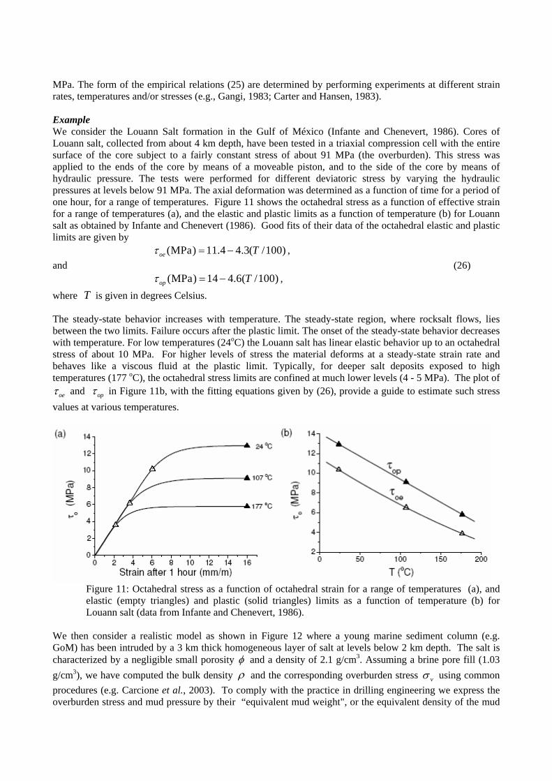
MPa. The form of the empirical relations (25) are determined by performing experiments at different strain rates, temperatures and/or stresses (e.g., Gangi, 1983; Carter and Hansen, 1983). Example We consider the Louann Salt formation in the Gulf of México (Infante and Chenevert, 1986). Cores of Louann salt, collected from about 4 km depth, have been tested in a triaxial compression cell with the entire surface of the core subject to a fairly constant stress of about 91 MPa (the overburden). This stress was applied to the ends of the core by means of a moveable piston, and to the side of the core by means of hydraulic pressure. The tests were performed for different deviatoric stress by varying the hydraulic pressures at levels below 91 MPa. The axial deformation was determined as a function of time for a period of one hour, for a range of temperatures. Figure 11 shows the octahedral stress as a function of effective strain for a range of temperatures (a), and the elastic and plastic limits as a function of temperature (b) for Louann salt as obtained by Infante and Chenevert (1986). Good fits of their data of the octahedral elastic and plastic limits are given by

(MPa) 11.4 4.3( /100)oe Tτ = − , and (26)

(MPa) 14 4.6( /100)op Tτ = − ,

where T is given in degrees Celsius. The steady-state behavior increases with temperature. The steady-state region, where rocksalt flows, lies between the two limits. Failure occurs after the plastic limit. The onset of the steady-state behavior decreases with temperature. For low temperatures (24oC) the Louann salt has linear elastic behavior up to an octahedral stress of about 10 MPa. For higher levels of stress the material deforms at a steady-state strain rate and behaves like a viscous fluid at the plastic limit. Typically, for deeper salt deposits exposed to high temperatures (177 oC), the octahedral stress limits are confined at much lower levels (4 - 5 MPa). The plot of

oeτ and opτ in Figure 11b, with the fitting equations given by (26), provide a guide to estimate such stress values at various temperatures.

Figure 11: Octahedral stress as a function of octahedral strain for a range of temperatures (a), and elastic (empty triangles) and plastic (solid triangles) limits as a function of temperature (b) for Louann salt (data from Infante and Chenevert, 1986).

We then consider a realistic model as shown in Figure 12 where a young marine sediment column (e.g. GoM) has been intruded by a 3 km thick homogeneous layer of salt at levels below 2 km depth. The salt is characterized by a negligible small porosity φ and a density of 2.1 g/cm3. Assuming a brine pore fill (1.03 g/cm3), we have computed the bulk density ρ and the corresponding overburden stress vσ using common procedures (e.g. Carcione et al., 2003). To comply with the practice in drilling engineering we express the overburden stress and mud pressure by their “equivalent mud weight", or the equivalent density of the mud

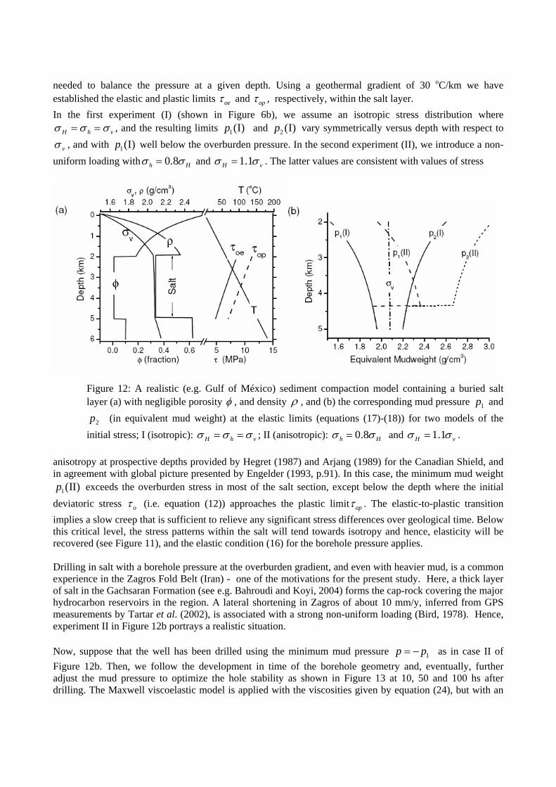
needed to balance the pressure at a given depth. Using a geothermal gradient of 30 oC/km we have established the elastic and plastic limits oeτ and opτ , respectively, within the salt layer. In the first experiment (I) (shown in Figure 6b), we assume an isotropic stress distribution where

H h vσ σ σ= = , and the resulting limits and vary symmetrically versus depth with respect to 1(I)p 2 (I)p

vσ , and with well below the overburden pressure. In the second experiment (II), we introduce a non-uniform loading with

1(I)p0.8h Hσ σ= and 1.1H vσ σ= . The latter values are consistent with values of stress

Figure 12: A realistic (e.g. Gulf of México) sediment compaction model containing a buried salt layer (a) with negligible porosity φ , and density ρ , and (b) the corresponding mud pressure and

(in equivalent mud weight) at the elastic limits (equations (17)-(18)) for two models of the initial stress; I (isotropic):

1p

2p

H h vσ σ σ= = ; II (anisotropic): 0.8h Hσ σ= and 1.1H vσ σ= . anisotropy at prospective depths provided by Hegret (1987) and Arjang (1989) for the Canadian Shield, and in agreement with global picture presented by Engelder (1993, p.91). In this case, the minimum mud weight

exceeds the overburden stress in most of the salt section, except below the depth where the initial deviatoric stress

1(II)p

oτ (i.e. equation (12)) approaches the plastic limit opτ . The elastic-to-plastic transition implies a slow creep that is sufficient to relieve any significant stress differences over geological time. Below this critical level, the stress patterns within the salt will tend towards isotropy and hence, elasticity will be recovered (see Figure 11), and the elastic condition (16) for the borehole pressure applies. Drilling in salt with a borehole pressure at the overburden gradient, and even with heavier mud, is a common experience in the Zagros Fold Belt (Iran) - one of the motivations for the present study. Here, a thick layer of salt in the Gachsaran Formation (see e.g. Bahroudi and Koyi, 2004) forms the cap-rock covering the major hydrocarbon reservoirs in the region. A lateral shortening in Zagros of about 10 mm/y, inferred from GPS measurements by Tartar et al. (2002), is associated with a strong non-uniform loading (Bird, 1978). Hence, experiment II in Figure 12b portrays a realistic situation. Now, suppose that the well has been drilled using the minimum mud pressure as in case II of Figure 12b. Then, we follow the development in time of the borehole geometry and, eventually, further adjust the mud pressure to optimize the hole stability as shown in Figure 13 at 10, 50 and 100 hs after drilling. The Maxwell viscoelastic model is applied with the viscosities given by equation (24), but with an

1p = − p

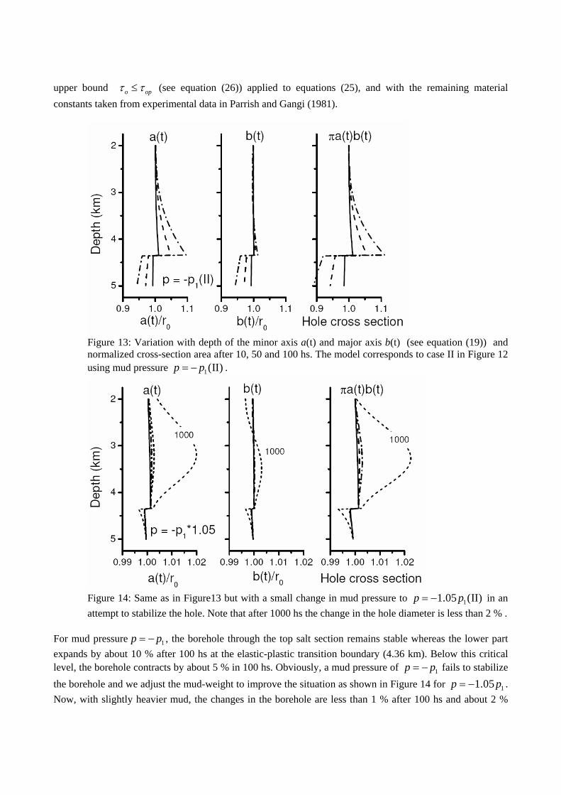
upper bound o opτ τ≤ (see equation (26)) applied to equations (25), and with the remaining material constants taken from experimental data in Parrish and Gangi (1981).

Figure 13: Variation with depth of the minor axis a(t) and major axis b(t) (see equation (19)) and normalized cross-section area after 10, 50 and 100 hs. The model corresponds to case II in Figure 12 using mud pressure . 1(II)p p= −

Figure 14: Same as in Figure13 but with a small change in mud pressure to in an attempt to stabilize the hole. Note that after 1000 hs the change in the hole diameter is less than 2 % .

11.05 (II)p p= −

For mud pressure , the borehole through the top salt section remains stable whereas the lower part expands by about 10 % after 100 hs at the elastic-plastic transition boundary (4.36 km). Below this critical level, the borehole contracts by about 5 % in 100 hs. Obviously, a mud pressure of fails to stabilize the borehole and we adjust the mud-weight to improve the situation as shown in Figure 14 for . Now, with slightly heavier mud, the changes in the borehole are less than 1 % after 100 hs and about 2 %

1p = − p

p1p = −

11.05p p= −

after 1000 hs, which normally should be sufficient time to drill and set the casing. Obviously, setting casing at the transition level would be required before drilling with reduced mud-weights in the lower section. The experiments above are in qualitative agreement with the in-situ measurements by caliper of shrinkage and expansion of a real well bore in a salt layer (probably Louann salt), as a function of time for three different mud-weights published by Kim (1988). for highly under-balanced mud (14.3 lb/gal) the hole (18" at 17700 ft) shrinkage was significant (2.3" in 12 hours), and by increasing the mud-weight (to 15.3 lb/gal) the shrinkage was reduced (0.6" in 12 hours). With heavier mud-weight (17.3 lb/gal), the caliper indicated stability or a slight expansion of the hole. For operational reasons, each experiment was terminated with only one caliper run after 12 hours. The data provided by Kim (1988) is thus not sufficient for a quantitative comparison with our theory.

CONCLUSION We have presented a case history of pressure and well-stability analysis based on well and seismic data. In an area of good seismic coverage with accurate velocity analysis the stress patterns are reasonable well expressed in the velocity cube and the seismic velocity field thus constitutes an important support in the pre-drill pressure and well-stability analysis. Despite complex stress patterns due to the combined action of salt tectonics and compaction disequilibrium, we have demonstrated that accurate pressure prediction from seismic and well data, in a Gulf of Mexico mini-basin next to a salt dome, is feasible using a classical soil- mechanical approach provided sufficient calibration data are available. For drilling through rocksalt we have developed a theoretical approach to analyze the stability of boreholes during and after drilling. We obtain expressions for the shape of the borehole-cross section, the borehole-wall closure time and the optimal mud-weight to avoid wall collapse and expansion. The theory describes transient creep by the Zener model and steady-state creep by the Maxwell model. The Zener model is used under pressure and temperature conditions, where the rock behaves as a viscoelastic solid. The choice depends on the value of the elastic octahedral stress which determines the limit separating transient flow from unrecoverable steady-state flow. Examples for the Louann Salt formation are given which are in qualitative agreement with published results for real in-situ experiments. ACKNOWLEDGMENTS This work is in supported by Norsk Hydro a.s. (Bergen, Norway) REFERENCES Arjang, B., 1989, Pre-mining stresses at some hard rock mines in the Canadian Shield. Rock mechanics as a guide for efficient utilization of natural resources: Proc. 30th US Symp. Rock Mechanics, 545-551, Balkema. Bahroudi, A. and H.A. Koyi, 2004, Tectono-sedimentary framework of the Gachsaran Formation in the Zagros foreland basin: Marine and Petroleum Geology, 21, 1295-1310. Baldwin, B. and Butler, C.O., 1985, Compaction curves, AAPG Bull., 69, 622-626. Barker, C., 1990, Calculated volume and pressure changes during the thermal cracking of oil to gas in reservoirs: AAPG Bull., 74, 1254-1261. Barker, J. W., and Meeks, W. R., 2003, Estimating fracture gradient in Gulf of México deepwater, shallow massive salt sections: SPE-84552 Ben-Menahem, A. and S. J. Singh, 1981, Seismic waves and sources, Springer-Verlag. Berg, R. R., and Gangi, A.F., 1999, Primary migration by oil-generation microfracturing in low-permeability source rocks: Application to the Austin chalk, Texas: AAPG Bull., 83, no. 5, 727–756.

Bird, P., 1978, Finite element modeling of lithosphere deformation: The Zagros collision orogeny: Tectonophysics, 50, 307-336. Bowers, G. L., 1995, Pore pressure estimation from velocity data, Accounting for overpressure mechanisms besides undercompaction, IADC/SPE Drilling Conf., #27488, 515-530. Bowers, G. , 2001, State of the art in pore pressure estimation, in DEA Project 119 Manual, Knowledge Systems Inc. Bowers, G. , 2001, State of the art in fracture gradient estimation, in DEA Project 119 Manual, Knowledge Systems Inc. Carcione, J. M., 2001, Wave Fields in Real Media.Theory and numerical simulation of wave propagation in anisotropic, anelastic and porous media, Pergamon Press. Carcione, J. M. and Gangi, A., 2000a, Non-equilibrium compaction and abnormal pore-fluid pressures: effects on seismic attributes, Geophys. Prosp., 48, 521-537. Carcione, J. M. and Gangi, A., 2000b, Gas generation and overpressure: effects on seismic attributes, Geophysics, 65, 1769-1769. Carcione, J. M. and Helle, H. B., 2002, Rock physics of geopressure and prediction of abnormal pore fluid pressures using seismic data, CSEG Recorder, (Sept. Issue) 8-30. Carcione, J. M., Helle, H. B, Pham, N. H. and Toverud, T., 2003, Pore pressure estimation in reservoir rocks from seismic reflection data: Geophysics, 68, 1569-1579. Carcione, J. M., Helle, H. B and Gangi, A. F., 2005, Theory of borehole stability when drilling through salt formations, Geophysics (in press) Carter, N. L., and Hansen, F. D., 1983, Creep of rocksalt: Tectonophysics, 92, 275-333. Dutta, N. C., 1983, Shale compaction and abnormal pore pressures: A model of geopressures in the Gulf of Mexico Basin, 53rd Ann, SEG Meeting. Dutta, N. C., and Levin, F. K., 1990, Geopressure, Geophysical Reprint Series No. 7, Society of Exploration Geophysicists. Eaton, B. A. 1976, Graphical method predicts geopressure worldwide, World Oil, July issue, 100-104. Eaton, B. A., and Eaton, T. L., 1997, Fracture gradient prediction for the new generation, World Oil, October issue, 93-100. Engelder, T.,1993, Stress regimes in the lithosphere: Princeton University Press. Fredrich, J.T., Coblentz, D., Fossum, A.F. and Thorne, B.J., 2003, Stress perturbation adjacent to salt bodies in the deepwater Gulf of Mexico: SPE 84554. Gangi, A. F., 1981, A constitutive equation for one-dimensional transient and steady-state flow of solids, Mechanical Behavior of Crustal Rocks, Geophysical Monograph 24, AGU, 275-285. Gangi, A. F., 1983, Transient and steady-state deformation of synthetic rocksalt: Tectonophysics, 91, 137-156.

Hegret,G., 1987, Stress assumption for underground excavation in the Canadian Shield: Int. J. Rock Mech. Min. Sci. Geomech. Abstr. 24, 95-97. Hubbert, M.K. and Willis, D.G., 1957, Mechanics of hydraulic fracturing, AIME Petroleum Transactions, 210, 153-168. Infante, E. F., and Chenevert, M. E., 1986, Stability of boreholes drilled through salt formations displaying plastic behavior: SPE-1553. Kim, C. M., 1988, Field measurements of borehole closure across salt formation: Implementing to well cementing, 63rd Annual Fall Technical Conference and Exhibition of the Society of Petroleum Engineering, 2-5. Klausner, Y., 1991, Fundamentals of continuum mechanics of soils, Springer-Verlag. Knowledge System INC., 2001, Best Practice Procedures for Predicting Pre-Drill Geopresssures in Deep Water Gulf of Mexico, DEA Project 119 Manual. Law, B. E., Ulmishek, G. F., and Slavin, V. I. (eds.), 1998, Abnormal pressures in hydrocarbon environments: AAPG Memoir 70. Luo, X., and Vasseur, G., 1996, Geopressuring mechanism of organic matter cracking: numerical modeling, AAPG Bull., 80, 856-874. Magara, K., 1978, Compaction and fluid migration: Practical Petroleum Geology. Development in Petroleum Science 9, Elsevier. Mann, D. M., and Mackenzie, A. S., 1990, Prediction of pore fluid pressures in sedimentary basins: Marine and Petroleum Geology, 7, 55-65. Parrish, D. K., and Gangi, A. F., 1981, A nonlinear least-squares technique for determining multiple-mechanism, high-temperature-creep flow laws: Geophys. Monogr. Am. Geophys. Union, 24, 287-298. Pennebaker, E.S., 1968, An engineering interpretation of seismic data, SPE # 2165. Rubey, W. W., and Hubbert, M. K., 1959, Role of fluid pressure mechanics of overthrust faulting, II. Overthrust belt in geosynclinal area of Western Wyoming in light of fluid pressure hypothesis, Geol. Soc. Am., 70, 167-205. Serata, S., and Gloyna, E. F., 1960, Principles of structural stability of underground salt cavities: J. Geophys. Res., 65, 2979-2987. Schlumberger, 1989, Log Interpreation: Principles / Application. Schlumberger Educational Services, Houston. Smith, J. E., 1971, The dynamics of shale compaction and evolution of pore-fluid pressure, Math. Geol., 3, 239-263. Tartar, M., D. Hatzfeld, J. Martinod, A. Walpersdorf, M. Ghafori-Ashtiany and J. Chéry, 2002, The present-day deformation of the central Zagros from GPS measurements: Geophys. Res. Lett., 29, 19. Terzaghi, K. and Peck, R.B., 1948, Soil Mechanics in Engineering Practice, Wiley, N.Y. Zener, C., 1948, Elasticity and anelasticity of metals, University of Chicago Press.