Probability and Irreversibility in Modern

Statistical Mechanics: Classical and Quantum

David Wallace

July 1, 2016

Abstract

Through extended consideration of two wide classes of case studies —dilute gases and linear systems — I explore the ways in which assump-tions of probability and irreversibility occur in contemporary statisticalmechanics, where the latter is understood as primarily concerned withthe derivation of quantitative higher-level equations of motion, and onlyderivatively with underpinning the equilibrium concept in thermodynam-ics. I argue that at least in this wide class of examples, (i) irreversibility isintroduced through a reasonably well-defined initial-state condition whichdoes not precisely map onto those in the extant philosophical literature;(ii) probability is explicitly required both in the foundations and in thepredictions of the theory. I then consider the same examples, as well as themore general context, in the light of quantum mechanics, and demonstratethat while the analysis of irreversiblity is largely unaffected by quantumconsiderations, the notion of statistical-mechanical probability is entirelyreduced to quantum-mechanical probability.

1 Introduction: the plurality of dynamics

What are the dynamical equations of physics? A first try:

Before the twentieth century, they were the equations of classicalmechanics: Hamilton’s equations, say,

qi =∂H

∂pipi = −∂H

∂qi. (1)

Now we know that they are the equations of quantum mechanics:1

1For the purposes of this article I assume that the Schrodinger equation is exact in quantummechanics, and that ‘wavefunction collapse’, whatever its significance, is at any rate not a dy-namical process. This clearly excludes the GRW theory (Ghirardi, Rimini, and Weber 1986;Pearle 1989; Bassi and Ghirardi 2003) and similar dynamical-collapse theories (see Albert(2000) for extensive consideration of their statistical mechanics); it includes the Everett inter-pretation (Everett 1957; Wallace 2012) and hidden-variable theories like Bohmian mechanics(Bohm 1952; Bohm and Hiley 1993; Durr, Goldstein, and Zanghi 1996); in Wallace (2016) Iargue that it includes orthodox quantum mechanics, provided ‘orthodoxy’ is understood viaphysicists’ actual practice.

1

that is, Schrodinger’s equation,

d

dt|ψ〉 = − i

hH |ψ〉 . (2)

This answer is misleading, bordering on a category error. Hamilton’s equations,and Schrodinger’s, are not concrete systems of equations but frameworks inwhich equations may be stated. For any choice of phase space or Hilbert space,and any choice of (classical or quantum) Hamiltonian on that space, we get aset of dynamical equations. In classical mechanics, different choices give us:

• The Newtonian equations for point particles (better: rigid spheres) inter-acting under gravity, generalisable to interactions under other potential-based forces;

• The simple harmonic oscillator equations that describe springs and othervibrating systems;

• Euler’s equations, describing the rotations of rigid bodies;

• Euler’s (other) equations, describing fluid flow in the regime where viscos-ity can be neglected.

• (With a little care as to how the Hamiltonian dynamical framework han-dles them), the field equations of classical electromagnetism and generalrelativity.

In quantum mechanics, we also have

• The quantum version of the Newtonian equations, applicable to (e.g.)nonrelativistic point particles interacting under some potential;

• The quantum version of the harmonic oscillator;

• The quantum field theories of solid-state physics, describing such variedsystems as superconductors and vibrating crystals;

• The quantum field theories of particle physics, in particular the StandardModel, generally thought by physicists to underly pretty much all phe-nomena in which gravity can be neglected and most in which it cannot.

All of these equations are widely used in contemporary physics, and all have beenthoroughly confirmed empirically in applications to the systems to which theyapply. And this is already something of a puzzle: how is it that physics doesn’tjust get by with one such system, the right such system? Even if that system isfar too complicated to solve in practice, that in itself does not guarantee us theexistence of other, simpler, equations, applicable in domains where the RightSystem cannot be applied? Any systematic understanding of physics has tograpple with the plurality of different dynamical equations it uses. Indeed, itmust grapple with the plurality of frameworks, for the classical equations, too,

2

remain in constant use in contemporary physics. The problem of ‘the quantum-classical transition’ is poorly understood if it is seen as a transition from onedynamical system (quantum mechanics) to another; it is, rather, a problem ofunderstanding the many concrete classical dynamical equations we apply in awide variety of different situations.

But even this account greatly understates the plurality of dynamics. Somemore examples still:

• The equations of radioactive, or atomic, decay.

• The Navier-Stokes equation, describing fluid flow when viscocity cannotbe neglected.

• The Langevin equation, a stochastic differential equation describing thebehaviour of a large body in a bath of smaller ones, and the related Fokker-Planck equation, describing the evolution of a probability distributionunder the Langevin equation.

• The Vlasov equation, describing the evolution of the particles in a plasma— or the stars in a cluster or galaxy — in the so-called “collisionless”regime.

• The Boltzmann equation, describing the evolution of the atoms or moleculesin a dilute (but not ‘collisionless’) gas.

• The Balescu-Lenard equation, describing the evolution of plasmas outsidethe collisionless regime.

• The master equations of chemical dynamics, describing the change inchemical (or nuclear) composition of a fluid when particles of one speciescan react to form particles of another.

It is (as we shall see) a delicate matter which of these equations is classical andwhich quantum. But at any rate, none of them fit into the dynamical frameworkof either Hamiltonian classical mechanics or unitary quantum mechanics. Infact, for the most part they have two features that are foreign to both:

1. They are probabilistic, either through being stochastic or, more commonly,by describing the evolution of probability distributions in a way that can-not be reduced to deterministic evolution of individual states. (In thequantum case, they describe the evolution of mixed states in a way thatcannot be reduced to deterministic — much less unitary — evolution ofpure states.)

2. They are irreversible: in a sense to be clarified shortly, they build in a cleardirection of time, whereas both Hamilton’s equations and the Schrodingerequation describe dynamics which are in an important sense time-reversal-invariant.

3

And again, these equations — and others like them — are very widely usedthroughout physics, and very thoroughly tested in their respective domains.

One can imagine a world in which physics is simply a patchwork of over-lapping domains each described by its own domain-specific set of equations,with few or no connections between them. (Indeed, Nancy Cartwright (1983,1999) makes the case that the actual world is like this.) But the consensus inphysics is that in the actual world, these various dynamical systems are con-nected: equation A and equation B describe the same system at different levelsof detail, and equation A turns out to be derivable from equation B (perhapsunder certain assumptions). Indeed, it is widely held in physics that prettymuch every dynamical equation can ultimately, in principle, be derived fromthe Standard Model, albeit sometimes through very long chains of inference vialots of intermediate steps.

I don’t think it does great violence to physics usage to say that (non-equilibrium) statistical mechanics just is the process of carrying out these con-structions, especially (but not only) in the cases where the derived equations areprobabilistic and/or irreversible. But in any case, in this paper I want to pursuea characterisation of the conceptual foundations of (non-equilibrium) statisticalmechanics as concerned with understanding how such constructions can be car-ried out and what additional assumptions they make. The main conceptualpuzzles then concern precisely (1) the probabilistic and (2) the irreversible fea-tures of (much) emergent higher-level dynamics; they can be dramatised as acontradiction between two apparent truisms:

1. Derivation of probabilistic, irreversible higher-level physics from non-probabilistic,time-reversal-invariant lower-level physics is impossible: probabilities can-not be derived from non-probabilistic inputs without some explicitly prob-abilistic assumptions, and more importantly, as a matter of logic time-reversal invariant low-level dynamics cannot allow us to derive time-reversal-noninvariant results.

2. Derivation of probabilistic, irreversible higher-level physics from non-probabilistic,time-reversal-invariant lower-level physics is routine: in pretty much all ofthe examples I give, and more besides, apparent derivations can be foundin the textbooks. And these derivations have novel predictive success,both qualitatively (in many cases, such as the Boltzmann, Vlasov andBalescu-Lenard equations, higher-level equations in physics are derivedfrom the lower level and then tested, rather than established phenomeno-logically and only then derived) and quantitatively (statistical mechanicsprovides calculational methods to work out the coefficients and param-eters in higher-level equations from lower-level inputs, and does so verysuccessfully).

I want to suggest that we can make progress on resolving this apparent paradoxthrough three related strategies:

1. Focussing on the derivation of quantitative equations of motion, ratherthan on the qualitative problem of how irreversibility could possibly emerge

4

from underlying microphysics. The advantage of the former strategy isthat we actually have concrete ‘derivations’ of irreversible, probabilisticmicrophysics all over modern statistical mechanics; identifying the actualassumptions made in those derivations, and in particular focussing in onthose assumptions which have a time-reversal-noninvariant character, isprima facie a much more tractable task than trying to work out in theabstract what those assumptions might be.

2. Looking at examples from (relatively) contemporary physics. Insofar asphilosophy of statistical mechanics has considered the quantitative fea-tures of non-equilibrium statistical mechanics, it has generally focussedon Boltzmann’s original derivation of the eponymous equation, and oflater attempts to improve the mathematical rigor of that equation whilstkeeping its general conceptual structure. But contemporary statistical me-chanics tends to treat the Boltzmann equation in a different (more explic-itly probabilistic) way, as well as incorporating a wide range of additionalexamples.

3. Engaging fully with quantum as well as classical mechanics. It is commonto see, in foundational discussions, the claim that the relevant issues goover from classical to quantum mutatis mutandis, so that we can get awaywith considering only classical physics. Sklar (1993, p.12) is typical:

the particular conceptual problems on which we focus — theorigin and rationale of probability distribution assumptions overinitial states, the justification of irreversible kinetic equations,and so on — appear, for the most part, in similar guise in thedevelopment of both the classical and quantum versions of thetheory. The hope is that by exploring these issues in the tech-nically simpler classical case, insights will be gained that willcarry over to the understanding of the corrected version of thetheory.

I will argue that this position, while defensible as regards irreversibility,fails radically for probability — something that could perhaps have beenpredicted when we recall that quantum theory is itself an inherently prob-abilistic theory.

In sections 2–6 I look at modern non-equilibrium statistical mechanics throughtwo detailed classes of example: dilute gases (including the famous Boltzmannequation, where I contrast a modern, probabilistic analysis (section 3) withBoltzmann’s own approach (section 4) and linear systems (in particular Brow-nian motion in an oscillator environment, which gives rise to the stochasticLangevin equation and the related Fokker-Planck equation). In both cases, thename of the game is to derive closed-form equations from some coarse-graineddescription of the system. And two common features of these derivations standout: explicit and irreducible appeal to the Liouville form of classical mechanics,and a concrete, quantitative condition for irreversibility expressed in terms of

5

an initial-state condition that constrains the residual (i. e. , non-coarse-grained)features.

In sections 7–12 I consider the quantum case, first in general terms (section7), where the analogy between quantum mixed states and classical probabilitydistributions turns out to be superficial, and then in the concrete context of thequantum versions of the dilute gas and of Brownian motion — where “quantumversion” does not mean “some new system, analogous to the old”, but “the sameold system, analysed correctly once we remember that quantum mechanics is thecorrect underlying dynamics”. I conclude that while the problem of irreversibil-ity looks pretty similar classically and quantum-mechanically, the problem ofprobability is radically transformed: statistical-mechanical probabilities reduceentirely to quantum-mechanical ones.

The physics discussed in this paper is standard and I do not give origi-nal references. I have followed Balescu (1997) (for dilute gases), Zeh (2007)and Zwanzig (1960, 1966) for the general linear-systems formalism, Zwanzig(2001) for the Langevin and Fokker-Planck equations, Paz and Zurek (2002) forthe perturbative derivation of the Fokker-Planck equation, Peres (1993) for thephase-space version of quantum mechanics, and Liboff (2003) for the quantumversion of the BBGKY hierarchy.

2 The BBGKY hierarchy and the Vlasov equa-tion

Consider N indistinguishable classical point particles (for very large N : 106 atleast, perhaps larger), interacting via the Hamiltonian

HN =∑

1≤i≤N

pi · pi2m

+∑

1≤i<j≤N

V (qi − qj)

≡ H1(pi,qi) +

∑1≤i<j≤N

V (qi − qj). (3)

With the right choices of the interaction term V , this might describe the particlesin a ‘classical’ gas or plasma, or the stars in a galaxy or cluster.

A standard move in contemporary statistical mechanics is to consider theevolution of a probability distribution ρ over phase space under the Hamiltoniandynamics defined by this Hamiltonian. (Thus probability is introduced explicitlyand by hand; I offer no justification for this at this stage, beyond the fact thatit is in fact routinely done!) It is well known that any such distribution evolvesby the Liouville equation,

d

dtρ = HN , ρ =

∑1≤i≤N

(∂HN

∂qi· ∂ρ∂pi− ∂HN

∂qi· ∂ρ∂pi

). (4)

If we assume the distribution ρ is symmetric under particle interchange (or,equivalently, if we just work with the symmetrised version of ρ, which is em-pirically equivalent), and if we write xi, schematically, for the six coordinates

6

qi,pi, then we can define, for each M ≤ N , the M -particle marginal probabilityas

ρM =∏

M<i≤N

∫dx iρ(x1, . . . xN ). (5)

ρm represents the probability that a randomly-selected M -tuple of particles willbe found in a given region of their M -particle phase space. We can, iteratively,define m-particle correlation functions: the 2-particle correlation function is

c2(x1, x2) = ρ2(x1, x2)− ρ1(x1)ρ1(x2), (6)

the three-particle correlation function is

c3(x1, x2, x3) = ρ3(x1, x2, x3)− ρ1(x1)ρ1(x2)ρ1(x3)

− ρ2(x1, x2)c2(x3)− ρ2(x1, x3)c2(x2)− ρ2(x2, x3)c2(x1) (7)

and so forth.The BBGKY hierarchy (named for Bogoliubov, Born, Green, Kirkwood

and Yvon) is a rewriting of the Liouville equation in terms of the n-particlemarginals. For each M , an equation of motion can be written down that isalmost a closed first-order differential equation for ρM , but which has a term inρM+1:

d

dtρM = HM , ρM

+ (N−M)∑

1≤i≤M

∫dxM+1∇V (qi − qM+1) · ∂ρM+1

∂pi(8)

So the first equation in the hierarchy can be used to determine the evolution ofρ1, but only given the value of ρ2; the latter can in turn be determined from thesecond equation, and so forth. For instance, the first equation in the hierarchy,

d

dtρ1 = H1, ρ1+ (N−1)

∫dx2∇V (q1 − q2) · ∂ρ2

∂p2, (9)

is the equation for free-particle motion plus a correction term linear in the two-particle marginal.

The last equation in the hierarchy is just the N -particle Liouville equation,and the full system of equations does not take us beyond that equation. Thevalue of the hierarchy is that it allows us to define various approximations. Ifwe can justify assuming that the M + 1-particle marginals are negligible, wecan truncate the hierarchy at the Mth equation and obtain a closed system ofequations for ρM . The grounds for that assumption will have to be assessedon a case-by-case basis, but crucially, any such assumption does not in itselfcontain any statement of time asymmetry.

For instance, the collisionless approximation takes c2 ' 0, i. e. ρ2(x1, x2) 'ρ1(x1)ρ1(x2) (and also N−1 ' N) and closes the first equation in the hierarchy

7

to give a self-contained equation in ρ1: the Vlasov equation,

d

dtρ1(q,p, t) = H1, ρ1 (q,p, t)+Nρ1(q,p, t)

∫dp′ dq′ ρ1(q′,p′, t)∇V (q−q′),

(10)widely used in plasma physics and galactic dynamics. This approximation isjustified by (a) assuming the initial multiparticle correlations are negligible;(b) making additional assumptions about the initial state and the dynamicswhich jointly entail that negligible multiparticle correlations remain negligible.Under these assumptions the equation, which on its face describes a one-particleprobability distribution, can also be taken to describe the actual distribution ofparticles when averaged over regions large compared to (total system volume /N).

I make no claim that the assumptions used to derive the Vlasov equationhave been rigorously demonstrated to entail it. But they don’t appear to differfrom the general run of the mill in mainstream theoretical physics in their levelof rigor. And, since they do not distinguish a direction of time, nor does theVlasov equation: it is probabilistic, but time-reversal-invariant. (It is, however,nonetheless highly non-trivial, despite its superficial resemblance to the one-particle version of the Poisson equation: in particular, the second term in theequation is non-linear in ρ1.) Irreversibility will require a more complicatedequation, to which I now turn.

3 The Boltzmann equation: a modern approach

Let’s relax the collisionless assumption, but only slightly: in the dilute-gas as-sumption, we assume that three-particle correlations are negligible. We alsoassume a two-particle interaction potential V that decreases rapidly with dis-tance, so that the nonlinear term in the Vlasov equation is negligible. The firsttwo equations in the BBGKY hierarchy are now a closed set of equations in ρ1

and c2, which after some manipulation (see Balescu (1997, ch.7) for the details)yields the following (schematically expressed) integro-differential equation forρ1:

d

dtρ1(t) = H1, ρ1+

∫ t

0

dτ K(τ)(ρ1 ⊗ ρ1)(t− τ) + Λ(t) · c2(0) (11)

Here I write (ρ1⊗ρ1)(x1, x2, t) ≡ ρ1(x1, t)ρ1(x2, t), and suppress the dependenceof ρ1 and c2 on anything except time. Λ(t) and K(t) are time-dependent linearoperators whose precise form will not be needed.

This equation holds only for t > 0, and might appear to describe explic-itly time-reversal-noninvariant dynamics. It does not: it has been derived fromthe dilute-gas approximation without further assumptions and the latter as-sumption is time-reversal (and time-translation) invariant. The time reverse ofthe equation holds for t < 0, and the whole system distinguishes no preferreddirection or origin of time.

8

It can now be demonstrated — and again, this is a mathematical result,the rigor of which can be questioned but which involves no additional physicalassumptions — that K(τ)ρ1 ⊗ ρ1(t − τ) decreases very rapidly with time, sothat (for times short compared to the recurrence time T of the system) we canapproximate the third term in (11) by∫ t

0

dτ K(τ)(ρ1 ⊗ ρ1)(t− τ) '

(∫ T

0

dτ K(τ)

)(ρ1 ⊗ ρ1)(t). (12)

And in fact the expression on the right hand side is equal to the well-knownBoltzmann collision term κ[σ, ρ1(t)], which depends on ρ1(t) (quadratically) andon the scattering cross-section σ(pp′ → kk′) for two-particle scattering underthe interaction potential V . (The latter can be calculated by standard methodsof scattering theory.)

The equation (11) can now be approximated as

d

dtρ1(t) = H1, ρ1(t)+ κ[σ, ρ1(t)] + Λ(t) · c2(0). (13)

This differs from the full Boltzmann equation,

d

dtρ1(t) = H1, ρ1(t)+ κ[σ, ρ1(t)], (14)

only by the final term Λ(t) · c2(0), which is a dependency of the rate of changeof ρ1 at time t on the initial two-particle correlation function.

In textbooks (see, e. g. , Balescu (1997, ch.7), one can find heuristic argu-ments to the effect that this term can be expected to be negligible (perhapsafter some short ‘transient’ period): indeed, Balescu quotes Prigogine and co-workers as referring to the Λ(t) · c2(0) term as the destruction term. But thisassumption needs to be treated cautiously: the Boltzmann equation is time-reversal noninvariant, and so the assumption that this term vanishes must insome way build in assumptions that break the time symmetries of the problem.And indeed, the heuristic arguments would fail if a precisely arranged patternof delicate correlations were present at time 0: they rely on certain assumptionsof genericity about those correlations.

Following Wallace (2010), let’s call an initial two-particle correlation func-tion (and, by extension, an initial probability distribution satisfying our otherassumptions) forward compatible if Λ(t)·c2(0) is negligible for at least 0 < t T .Then we have established that systems whose initial state is forward compatiblewill obey the Boltzmann equation.

How are we to think about this assumption? I can see three options:

1. At one extreme, we could simply posit that a system’s state is forwardcompatible, and derive from this that it obeys the Boltzmann equation.This is dangerously close to circularity: to say that a state is forwardcompatible is close to saying just that it obeys the Boltzmann equation.The formal machinery developed here allows us to sidestep that circularity:

9

to say that a correlation function satisfies Λ(t) · c2(0) ' 0 is equivalentto saying that its forward time evolution satisfies the Boltzmann equationonly given significant, non-trivial mathematical work. But we are still leftwith little clarity as to what this obscure mathematical expression means,and in particular, we fail to connect to the heuristic arguments that thisterm can in some sense be ‘expected’ to vanish for ‘reasonable’ choices ofc2(0).

2. At the other extreme, we could exploit the linearity of Λ(t) to observe thatif c2(0) vanishes, the troublesome term is removed entirely. So this state,at least, is certainly forward compatible: positing that the initial state isuncorrelated thus suffices to guarantee that the Boltzmann equation holdsfor 0 < t T . However, it is much stronger than is required (we expectthat a great many other choices of correlation are also forward compat-ible) and somewhat physically implausible (a totally uncorrelated dilutegas will swiftly build up some correlations, and indeed we can write anexplicit equation for them; if they really were negligible at all times, theBoltzmann equation would reduce to the Vlasov equation). And again,this assumption fails to engage with the heuristic arguments for the van-ishing of Λ(t) · c2(0) for ‘reasonable’ initial states.

3. An intermediate strategy (suggested in Wallace (2010)) is to assume Sim-plicity : the assumption that the initial state’s correlations can be de-scribed in a reasonably simple mathematical form. (We need to explic-itly bar descriptions that involve starting with a simple sate, evolving itforward, and then time-reversing it!) We have heuristic, but extremelystrong, grounds to assume that Simple states are forward compatible.

The second and third of these assumptions, counter-intuitively, are time-reversalinvariant: Simple states time reverse to simple states, uncorrelated states touncorrelated ones. But they are not time translation invariant: their forwardand backward time evolutes violate the condition. Imposing either conditionguarantees (or, for the simplicity assumption, is heuristically likely to guarantee)that the Boltzmann equation holds for 0 < t T , and that its time reverseholds for 0 > t > −T . So such conditions can only be imposed at the beginningof a system’s existence, on pain of experimental disconfirmation.

Superficially, it is easy to make the argument that simplicity, at least, cannaturally be expected from a physical process that creates a system: such pro-cesses cannot plausibly be expected to generate delicate patterns of correlations.(The same might be said for the straightforward assumption of forward com-patibility.) But again, this is not innocent: the time reversal of a system’s finalstate, just before its destruction, is certainly not forward compatible, and soour argument builds in time-directed assumptions. Assuming that we seek adynamical explanation for irreversibility (and are not content, for instance, toappeal to unanalysable notions of agency or causation) then a familiar regressbeckons, and we are led to assume some condition analogous to forward com-patibility or simplicity, applied to the very early Universe. (I discuss this issue

10

in more detail in Wallace (2010).)In any case, for the purposes of this paper, what matters is that we have

identified the time-asymmetric assumption being made in (a modern derivationof) the Boltzmann equation: it is an assumption about the initial condition ofthe system, phrased probabilistically (it is a constraint on the two-particle corre-lation function, which is inherently probabilistic) and with no implications as tothe bulk distribution of particles in the system (insofar as these are coded by theone-particle marginal, given that all higher-order correlations are small). It willbe instructive to compare this to the situation in Boltzmann’s own derivationof the Boltzmann equation.

4 The Boltzmann equation: contrast with thehistorical approach

The equation derived by Boltzmann himself2 has the same functional form aswhat I have called the Boltzmann equation (albeit Boltzmann confined his at-tention to the case where ρ1 is spatially constant, so that the free-particle termH1, ρ1 vanishes). But its interpretation is quite different. To Boltzmann, ρ1

was not a probability distribution: it was a smoothed version of the actual dis-tribution function of particles over 1-particle phase space, so that ρ1(q,p)δV isthe actual fraction of particles in a region δV around (q,p). (The smoothing isnecessary because, with a finite number of point particles, ρ1 would otherwisejust be a sum of delta functions.)

Boltzmann makes a number of simplifying assumptions about the dynam-ics (notably: that collisions are hard-sphere events; that three-body collisionscan be neglected; that long-distance interactions can be neglected) which aretime-reversal invariant and broadly equivalent to the time-reversal-invariantassumptions made in the modern derivation. He then assumes the famousStosszahlansatz (SZA): the assumption that the subpopulation of particles whichare about to undergo a collision has the same distribution of momenta as thepopulation as a whole. Given this assumption, imposed over a finite time inter-val [0, τ ], he then deduces that over that time interval the Boltzmann equationholds. The assumption is thus explicitly time-reversal-noninvariant: assumingthat ρ1 is not stationary, if it holds over an interval then its time reverse cannothold over that interval. (If it did, then both the Boltzmann equation and itstime reverse would hold over that interval, contradicting Boltzmann’s famousH-theorem, which tells us that the function H[ρ] monotonically increases duringthe evolution of any non-stationary distribution under the Boltzmann equation.)

From a formal perspective, the probabilistic derivation in section 3 has sig-nificant advantages over the historical approach. (Perhaps unsurprisingly, giventhat it has in fact largely supplanted the historical approach in theoreticalphysics.) In particular:

2Here I follow Brown et al ’s (2009)’s account of Boltzmann’s work; see that paper fororiginal references.

11

1. The SZA is a condition that must hold throughout an interval of time ifthat system is to obey the Boltzmann equation over that interval of time.But whether a condition holds at time t > 0 is dynamically determinedby the system’s state at time 0, and Boltzmann’s derivation provides littleinsight as to what constraint on the state at time 0 suffices to impose theSZA at later times. Lanford’s celebrated proof of the Boltzmann equation(Lanford (1975, 1976, 1976); carefully discussed by Valente (2014) andUffink and Valente (2015)) demonstrates that imposing (a generalisationof) the SZA at time 0 suffices to guarantee that it holds over some [0, τ ]— but τ is extremely short, only a fifth of a mean free collision time.

By contrast, the probabilistic approach provides an explicit condition —Λ(t) · c2(0) ' 0 for 0 < t < T — for when the Boltzmann equation holds,and allows us to state in closed form at least one correlation function —c2(0) = 0 — that guarantees that the condition will continue to hold.(To be fair, Lanford’s results are at a much higher level of rigor than theprobabilistic derivation, so a reader’s assessment of this point will dependon their degree of tolerance of the mathematical practices of mainstreamtheoretical physics.)

2. The framework of the probabilistic approach readily generalises. On slightlydifferent assumptions about the dynamics, for instance, it leads to Lan-dau’s kinetic equation (governing weak collision processes) or to the Lenard-Balescu equation (governing collisional plasmas). Boltzmann’s originalapproach does not seem to have offered a comparably effective frameworkfor the construction of other statistical-mechanical equations.

3. Most significantly, and as I will discuss further in section 10, the probabilis-tic approach readily transfers to quantum mechanics, where Boltzmann’soriginal approach appears to fail completely.

Against this, Boltzmann’s original approach might be thought to have amajor conceptual advantage over the probabilistic approach, precisely becauseit eschews problematic notions of probability that seem to have no natural placein classical mechanics given that the latter features a deterministic dynamics.(Harvey Brown presses the point in his contribution to this volume.) To be blunt(the critic might say) then if progress in theoretical physics has moved fromBoltzmann’s original, relative-frequency, conception of the Boltzmann equationto a conception that relies on a mysterious concept of objective probability, thenso much the worse for progress.

In my view, the ultimate resolution of this problem is quantum-mechanical:when we consider quantum statistical mechanics, these probabilities receive anatural interpretation. But even setting quantum theory aside, it is not obvi-ous that the criticism is well-founded. For one thing, probabilistic notions arefrequently appealed to in discussions of the Boltzmann equation, even wherethe latter is understood a la Boltzmann: see Brown et al (2009) as regardsBoltzmann’s own derivation, and Uffink and Valente (2015) in the context ofLanford’s more rigorous analysis. So it is not after all clear that some notion of

12

probability is not required — in which case, why object to incorporating it intothe equations themselves?

More importantly, conceptual analyses have to answer to the actual shapeof theoretical physics, at least insofar as the latter is empirically successful. Ihave already noted that several generalisations of the Boltzmann equation canbe derived within the probabilistic framework but (so far as I know) have notbeen demonstrated within Boltzmann’s conception of the equation.

Now, these equations, whatever their derivation, are expressions of the one-particle marginal and can be reinterpreted without empirical consequence asequations in the actual relative frequency of particles’ phase-space locations.But classical statistical mechanics also offers examples where the predictions ofthe theory are themselves probabilistic in nature. In the next section, I presentone such example; it will also serve as a demonstration that the analysis ofirreversibility in section 3 is more general than just the Boltzmann equation.

5 Mori-Zwanzig projection and the Fokker-Planckequation

Let’s now consider a different Hamiltonian:

H(Q,P, q, p) =P 2

2M+ V (Q) +

∑1≤i≤N

ωi(qi2 + p2

i ) +∑

1≤i≤N

λiQqi (15)

(where functional dependence on q, p schematically depicts dependence on allof the qi, pi). This describes a single particle in one dimension (with position Qand momentum P ) (the ‘system’) interacting with a bath of harmonic oscillators(the ‘environment’); it is one common model for Brownian motion. Again weintroduce probabilities explicitly via a probability density ρ over the phase spacefor the N + 1 particles, and take Liouville’s equation as the basic dynamicalequation for this system. That distribution can be decomposed as

ρ(Q,P, q, p) = ρS(Q,P )ρE(q, p) + C(Q,P, q, p) (16)

where ρS and ρE are, respectively, the marginal probability distributions oversystem and environment, and C is the correlation function between the two.

Heuristically we might hope to find:

• that there is an autonomous dynamics for the single particle (assumingthat it is massive compared to the bath particles and that there are verymany of the latter, so that their influence is a kind of background noise);

• that the environment marginal ρE is pretty much constant during thesystem’s evolution, provided that it starts off invariant under the self-Hamiltonian

HE =∑

1≤i≤N

ωi(qi2 + p2

i ) (17)

of the bath.

13

With that in mind, we define the following projection map on the space ofdistributions:

Jρ(Q,P, q, p) = ρS(Q,P )E(q, p). (18)

Here ρS is the system marginal distribution of ρ, and E is some fixed distributionfor the environment, satisfying

HE , E = 0. (19)

(Typically we take E to be the canonical distribution for some given tempera-ture.) Then we can write ρ itself as

ρ = Jρ+ (1− J)ρ ≡ ρr + ρi. (20)

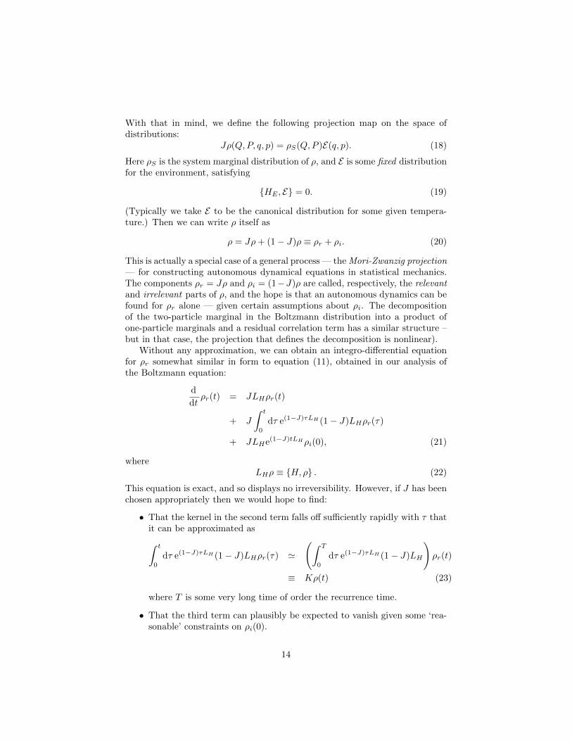
This is actually a special case of a general process — the Mori-Zwanzig projection— for constructing autonomous dynamical equations in statistical mechanics.The components ρr = Jρ and ρi = (1−J)ρ are called, respectively, the relevantand irrelevant parts of ρ, and the hope is that an autonomous dynamics can befound for ρr alone — given certain assumptions about ρi. The decompositionof the two-particle marginal in the Boltzmann distribution into a product ofone-particle marginals and a residual correlation term has a similar structure –but in that case, the projection that defines the decomposition is nonlinear).

Without any approximation, we can obtain an integro-differential equationfor ρr somewhat similar in form to equation (11), obtained in our analysis ofthe Boltzmann equation:

d

dtρr(t) = JLHρr(t)

+ J

∫ t

0

dτ e(1−J)τLH (1− J)LHρr(τ)

+ JLHe(1−J)tLHρi(0), (21)

whereLHρ ≡ H, ρ . (22)

This equation is exact, and so displays no irreversibility. However, if J has beenchosen appropriately then we would hope to find:

• That the kernel in the second term falls off sufficiently rapidly with τ thatit can be approximated as∫ t

0

dτ e(1−J)τLH (1− J)LHρr(τ) '

(∫ T

0

dτ e(1−J)τLH (1− J)LH

)ρr(t)

≡ Kρ(t) (23)

where T is some very long time of order the recurrence time.

• That the third term can plausibly be expected to vanish given some ‘rea-sonable’ constraints on ρi(0).

14

Given the first assumption, and defining

Λ(t) = JLHe(1−J)tLH , (24)

we are left with the equation

d

dtρr(t) = JLHρr(t) +Kρr(t) + Λ(t)ρi(0) (25)

which is very similar in form to the proto-Boltzmann equation (13). No time-asymmetric assumption has been made to get this far; we now have to make aninitial-time assumption about ρi(0) to guarantee that ρi(0) is forward compat-ible, i. e. that Λ(t)ρi(0) ' 0 for 0 < t < T . As with the Boltzmann case, we canguarantee this by taking ρi(0) = 0; as with the Boltzmann case, this is usuallyoverkill.

Returning to the specific case of the oscillator bath, we can calculate thesecond term approximately by working to second order in perturbation the-ory. Given a forward-compatible initial state (which, in this case, will typicallyrequire at least that ρE(0) = E), we get the equation

d

dtρS(t) = HS , ρS(t)+η X,PρS(t)+α X, X, ρS(t)+f X, P, ρ (26)

whereHS = P 2/2M + V (Q) + ∆V (Q) (27)

and ξ, η, f and ∆Q are (somewhat complicated) functions of the λi coefficientsand the frequencies ωi of the oscillator bath. For reasonable assumptions, fis usually negligible; equation (26) is then the Fokker-Planck equation, and wecan get insight into it by recognising that it is the equation for the probabilitydistribution of a particle evolving under the Langevin equation, the stochasticdifferential equation

˙Q(t) = P (t)/M ; P (t) = −ηP (t) + ξ(t) (28)

where ξ(t) is a random variable satisfying

〈ξ(t)〉 = 0; 〈ξ(t1)ξ(t2)δt2〉 = 2αδt. (29)

(For details of both, see Zwanzig (2001, chs.1-2).)These equations — which are highly effective at describing the physics of

Brownian motion — make explicitly probabilistic predictions: for instance, thatthe root-mean-square value of the particle’s distance from its starting place aftertime t is (after an initial transient phase) equal to 2αt/η2. Unlike the case ofBrownian motion, the equations cannot be reinterpreted as non-probabilisticequations concerning the relative frequency of particles in a single system.

Incidentally, since the underlying Hamiltonian of this system is quadratic,the appeal to second-order perturbation theory is dispensible: with a bit of care,we can solve it exactly and confirm the approximate validity of equation (26).See Paz and Zurek (2002) for details.

15

6 Classical statistical mechanics: could do bet-ter?

I began with the observation that non-equilibrium statistical mechanics is con-cerned with establishing the relations between dynamical equations at differentlevels of description, especially in the cases where the higher-level equations areprobabilistic and/or irreversible; I noted that it is mysterious how probabilityor irreversibility can be derived from an underlying dynamics which has neitherfeature, but that paying attention to the details of such derivations might beilluminating.

We have now seen two such derivations in detail (conceptual detail at anyrate; the mathematics was left schematic), and I have argued that

1. The probabilistic features of the equations of statistical mechanics are notreadily removable: even in the case of the Boltzmann equation, which canbe reinterpreted as a non-probabilistic equation, its derivation is betterunderstood and more readily generalised when understood probabilisti-cally, and in the case of the Fokker-Planck and Langevin equations, theequations cannot even be reinterpreted non-probabilistically.

2. The irreversibility of at least a wide class of classical statistical-mechanicalequations (specifically, those which are either derived from the BBGKYhierarchy via the same approximation scheme we used for the Boltzmannequation, or derived by the Mori-Zwanzig method from a linear projection)can be tracked to a cleanly-stated assumption about the initial microstate— an assumption, however, which is again stated probabilistically.

3. No clue has been gleaned about the origins of the probabilities used inthese equations: in each case, our starting point was the Louville equation,applied to a probability distribution placed by fiat on phase space.

So we are in the unsatisfactory position of having acquired considerable evidenceas to the importance and ineliminability of probabilities in non-equilibrium sta-tistical mechanics, without gaining any insight at all into the origins of theseprobabilities. In the rest of the paper, I will demonstrate that this dilemmais resolved, or at least radically transformed, when we move from classical toquantum mechanics.

7 Mixed states and probability distributions inquantum statistical mechanics

At first sight, there is a straightforward translation scheme between classical andquantum that maps the previous section’s results directly across to quantumtheory. To phase-space points correspond Hilbert-space rays. To Hamilton’sequation corresponds Schrodinger’s. To probability distributions on phase space

16

correspond density operators. To Liouville’s equation corresponds its quantumcounterpart,

ρ = LHρ =df

i

h[ρ,H] . (30)

Appearances, however, can be deceptive.Von Neumann originally introduced the density operator to represent igno-

rance of which quantum state a system is prepared in: the idea is that if thesystem is prepared in state |ψi〉 with probability pi, then for any measured

observable X its expectation value is

〈X〉 =∑i

pi 〈ψi|X |ψi〉 = Tr

[X

(∑i

pi |ψi〉 〈ψi|

)], (31)

so that if we defineρ =

∑i

pi |ψi〉 〈ψi| , (32)

the formula 〈X〉 = Tr(Xρ) neatly summarises our empirical predictions. Butit was recognised from the start that (32) cannot be inverted to recover the piand |ψi〉: many assignments of probabilities to pure states give rise to the sameρ. By contrast, for any two distinct probability distributions over phase spacethere is (trivially) some measurement whose expectation value is different onthe two distributions.

(It is true that if we add the extra information that the |ψi〉 are orthogonal,and if we assume that ρ is non-degenerate, then the pi and the |ψi〉 can afterall be recovered. But (i) there is no particular problem in making sense ofprobability distributions over non-orthogonal states; (ii) the density operatorsused in statistical mechanics — particularly the microcanonical and canonicaldistributions — are massively degenerate.)

That’s a puzzling disanalogy, to be sure, but hardly fatal. In these post-positivist days, surely we can cope with a little underdetermination? But itgets worse. For recall: a joint state of system A and system B is genericallyentangled : it cannot be written as a product of pure states, and indeed there isno pure state of system A that correctly predicts the results of measurementsmade on system A alone. Indeed, the correct mathematical object to representthe state of system A alone, when it is entangled with another system, is againa density operator ρ, obtained by carrying out the partial trace over the degreesof freedom of system B. (But this density operator cannot be understood as aprobabilistic mixture of pure states, on pain of failing to reproduce in-principle-measureable Bell-type results.)

The corollary is that we can only represent a quantum system (or, indeed,our information about a quantum system, if that’s your preferred way of under-standing probabilities here) by a probability measure over pure states if withprobability 1 the system is not entangled with its surroundings. And in the caseof the macroscopically large systems studied in statistical mechanics, this is awildly implausible assumption: even if for some (already wildly implausible) rea-son we were confident that at time 0 there was no entanglement between system

17

and environment, some will develop extremely rapidly. (But note, conversely,that simply assuming (or idealising) that the system is currently dynamicallyisolated from its surroundings in no way rules out the possibility that it is en-tangled with them.)

If we want to place a probability measure over states of a system, then, ingeneral the only option will be to place it over the system’s possible mixed states.Mathematically, that’s straightforward enough: if a system has probability piof having mixed state ρi, then the expected value of a measurement of X is

〈X〉 =∑i

piTr(Xρi) = Tr

[X

(∑i

piρi

)]. (33)

But is clear that we get the exact same predictions by simply assigning thesystem the single mixed state

∑i piρi. In other words, probability distributions

over mixed states are indistinguishable from individual mixed states.Note how different this is from the classical case. Even formally (never mind

conceptually), the move from phase-space dynamics to distributional dynamicsis an extension of the mathematical framework of classical physics. But inquantum mechanics, the move from pure states to density operators is forcedupon us by considerations of entanglement quite independently of any explicitprobabilistic assumption, and so there is nothing formally novel about theirintroduction in statistical mechanics.

Put another way, any mathematical claim in quantum statistical mechanicscan be interpreted as a claim about the actual (perhaps mixed) state of thesystem. Nothing formally requires us to interpret it as any kind of probabilitydistribution over quantum states.

Now, perhaps this would be unimpressive if the foundations of quantum sta-tistical mechanics made major conceptual use of probabilistic ideas in derivingtheir results: if, for instance, the arguments given for the mathematical form ofquantum statistical equilibrium relied on probabilistic ideas. But a casual pe-rusal of the (fairly minimal) literature on quantum statistical mechanics servesto disabuse one of this notion. From Tolman’s classic text Tolman (1938) tomodern textbook discussions, the norm is to start with classical statistical me-chanics and then move from a probability distribution over phase-space pointsto a probability distribution over eigenstates of energy drawn from a particularbasis. I don’t really know any way to make sense of this, but certainly it can’tbe made sense of as a probability distribution over possible states of the systemgiven that (a) there is absolutely no reason, given the massive degeneracy thattypically characterises the Hamiltonian of macroscopic systems, to prefer oneenergy basis over another; (b) there is no a priori reason, even ignoring entan-glement, to assume with probability 1 that the system is in an eigenstate ofenergy; (iii) we shouldn’t ignore entanglement anyway, so assuming the systemis in any pure state is unmotivated.3

3Very occasionally (the only place I know is Binney et al (1992)) it is observed thata probability distribution uniform over all pure states with respect to the natural(unitary-

18

This is not to say that there is not high-quality, rigorous work on the foun-dations of quantum statistical mechanics, or even on the form of the equilib-rium distributions (for recent examples see Goldstein et al (2006), Malabarbaet al (2014), and Short (2011)). But insofar as these arguments avoid the abovefallacies, they do so because they try to establish (or at any rate can be in-terpreted as trying to establish) that the actual mixed state of a system atequilibrium is the microcanonical or canonical ensemble, not that the correctprobability distribution over such states reproduces that ensemble.

I conclude that there is no justification, and no need, for interpreting themixed states used routinely in quantum statistical mechanics as any kind ofprobability distribution over quantum states, rather than as the (mixed) quan-tum states of individual systems. And if that is the case, then — since inthe real world “classical” systems are just quantum systems that we can getaway with approximating as classical — it becomes at least very tempting tointerpret the ‘probability’ distributions of classical mechanics simply as classicallimits of individual quantum states, without any need at all for a distinctivelystatistical-mechanical conception of probability.

In fact — at least for the non-equilibrium systems we have considered so far— this move is not just tempting, but compulsory. As we will see, it is simplynot viable to interpret these systems as probability distributions over localisedquasi-classical systems, once quantum mechanics is taken into account.

8 The quantum mechanics of dilute gases

The dilute gas of hard spheres is the paradigm example in classical statisticalmechanics, both in considering the approach to equilibrium (the Boltzmannequation assumes this system) and in analysing equilibrium itself. But whathappens when quantum mechanics is used to analyse a system of this kind?

Let us begin with some parameters. The typical gas at standard temperatureand pressure has a molecular mass of around 10−26 or 10−27 kg, a molecularscale of around 10−10 m, a density of about 1 kg m−3, and typical molecularvelocities of around 102 or 103 m s−1; for definiteness, let’s assume our gas isconfined in a 1m3 box, and that it consists of 1027 hard spheres of mass 10−27

kg and cross-sectional area 10−20m2 moving at a mean speed of 103 m s−1.If classical microdynamics is to be a good approximation for this system,

presumably this means that the particles in the gas must be, and remain, lo-calised. So let’s start the system off in some (probably unknown) state in whicheach molecule is a localised wavepacket with a reasonably definite position andmomentum. We can now use approximately classical means to consider howthose wavepackets evolve prior to their first collisions.

Elementary methods tell us that for a gas with these parameters, the meanfree path — the mean distance travelled by a given particle before it collides

invariant) measure on states gives the same density operator as a distribution uniform over aparticular orthonormal basis, and that this is the justification for the latter; even here, though,the problem of mixed states is left unanswered.

19

with another — is 10−7m. The typical particle will cover this distance in 10−10

seconds.How wide will its wavepacket be at that time? Let its original width be

∆q(0), so that its initial spread ∆p in momentum is at least∼ h/∆q(0). Roughlyspeaking, its additional spread in position as a result of this spread in momentumafter time t will be t×∆p/m, so that its total spread after time t is given by

∆q(t) = ∆q(0) + t∆p/m = ∆q(0) +ht

m

1

∆q(0)(34)

Elementary calculus then tells us that this is minimised for ∆q(0) =√ht/m,

so that∆q(t) ≥ 2

√ht/m. (35)

For the parameters governing our ideal gas, this means that the minimum sizeof the packet after collision is approximately 3× 10−8 m.4

But this is thirty times the diameter of the molecule! To a rough approxi-mation, the first set of scattering events in our dilute gas will be well modelledby plane-wave scattering off a hard-sphere scattering surface. The resultantjoint state of two scattering particles will be a sum of two terms: one (muchthe larger one) corresponding to the state of the two particles in the absence oftheir interaction, and one an entangled superposition of the particles after scat-tering, with significant amplitude for any direction of scattering. Each particle’sindividual mixed state will be highly delocalised.

This is fairly obviously nothing like the classical microdynamics, in whicheach pair of particles deterministically scatters into a specific post-collision statedetermined entirely by the pre-collision state. A quantum-mechanical dilute gas,even if it is initially highly localised, rapidly evolves into a massively entangledand massively delocalised mess. So the classical microdynamics that underpinsthe derivation of Boltzmann’s equation (either in the ‘modern’ form I presentedin section 3, or in Boltzmann’s original derivation) is wildly false for real, phys-ical gases.

Let’s be clear about what we have learned here. The point is not thatthere are quantum regimes where the classical Boltzmann equation breaks down.There are such regimes, of course: the statistical mechanics literature is repletewith discussions of “quantum” gases, but in general this refers to situationswhere the intermolecular interaction has some complex quantum form, or (moreusually) where the gas is sufficiently dense that the effects of Bose-Einstein orFermi-Dirac statistics come into play, or where (as in the photon or phonongas) particle number is not conserved. But I am not considering that situation;nor am I considering the situations where the quantum Boltzmann equation isappropriate (as discussed by Brown, this volume). There is abundant empiricalevidence that the particle distribution in ordinary, nonrelativistic, dilute gases

4Don’t be fooled into thinking that ‘decoherence’ will somehow preserve localisation to agreater degree than this. These are microscopic particles: they don’t decohere, or rather: theirdecoherence is caused by their collision with other particles, and we’re explicitly consideringthe between-collision phase.

20

is governed by the classical Boltzmann equation — and yet, we have seen thatin those gases, the microdynamics assumed in the derivations of that equationis simply incorrect.

Why, then, do these derivations work? To address this question, it will beuseful to adopt a representation of quantum-mechanical systems as functionson phase space (as distinct from the usual representations on configuration ormomentum space); doing so will also cast light more generally on the relationbetween quantum states and classical probability distributions.

9 The quantum/classical transition on phase space

In the position representation of a quantum state, information about the prob-ability of a given result on a position measurement can be readily read off thequantum state via the mod-squared amplitude rule, whereas information aboutresults of momentum measurements are encoded rather inaccessibly in the phasevariation of the wavefunction. In the momentum representation, the reverse istrue. A phase space representation can be seen as enabling us to more readilyaccess both lots of information.

An alternative way of understanding quantum mechanics on phase space ismore direct: if the position representation is optimised for position measure-ments, and the momentum representation for momentum measurements, howcan we represent the state in a way optimised for phase-space measurements?One immediate objection is that the uncertainty principle forbids joint mea-surements of position and momentum; in fact, though, it forbids only sharpjoint measurements. The by-now well-established formalism of “positive op-erator valued measurements” (POVMs) allows for a wide variety of unsharpmeasurements, including phase-space measurements.

Indeed, we can straightforwardly write down such a family of phase spacemeasurements: choose any wave-packet state |Ω〉, reasonably well localized inposition and momentum but otherwise arbitrary (Gaussians are good choices)and let |q,p〉 denote the state obtained by translating the original state firstby q in position and then by p in momentum. (Here q and p are vectorsrepresenting the M position and M momentum coordinates of our system; if itconsists of N particles, for instance, M = 3N .) Then the (continuously infinite)family of operators (2π)−M |q,p〉 〈q,p| is a POVM. (See appendix for proof; theequivalent result for Gaussian choices of the wavepacket is standard, but I amnot aware of a proof in quite this form.) Since these wavepacket states are notorthogonal, they do not define a sharp measurement; however, if we partitionphase space into disjoint cells Ci which are large compared to the spread ofthe wave-packet state (and thus, at a minimum, large compared to hM ), theoperators

Πi =

∫Ci

|q,p〉 〈q,p| (36)

will approximately satisfyΠiΠj ' δijΠi. (37)

21

The Husimi function, defined for quantum state ρ by

Hρ(q,p) = (2π)−M 〈q,p| ρ |q,p〉 , (38)

can thus be consistently interpreted as a phase-space probability distributionprovided we do not probe it on too-small length scales. In fact, the Husimifunction can be inverted to recover |ψ〉, so in principle we could use it as ourphase-space representation; however, for our purposes it is inconvenient, and abetter choice is the Wigner function,

Wρ(q,p) =1

(hπ)M

∫dx e2ip·x/h 〈q−x| ρ |q+x〉 . (39)

The mathematical form of the Wigner function is not transparently connectedwith anything physical, but in fact, if we use the Wigner function (which is real,though not necessarily positive) as a probability measure, it will approximatelygive the correct phase-space measurement probabilities if averaged over regionslarge compared to hM . (Indeed, the Husimi function can be obtained from theWigner function merely by smearing it in position and momentum with therespective mod-squared wavefunctions of the wavepacket state; one advantageof the Wigner function is that it abstracts away from the need to specify aparticular choice of wavepacket state.)

The main virtue of the Wigner function is that its dynamics can be conve-niently compared to the classical case. Recall that classical probability distri-butions evolve by Liouville’s equation:

ρ = H, ρ . (40)

Transforming the Schrodinger equation to the Wigner representation tells usthat the Wigner function satisfies

W = H,WMB =df

2i

hsin

(h

2i·, ·

)· (H,W ). (41)

Here ·, ·MB , the Moyal bracket, is best understood via its series expansion:assuming H has the standard kinetic-energy-plus-potential-energy form, we canexpand it as

W = H,WMB = H,W+h2

24

∂3V

∂q3

∂3W

∂p3+O(h4). (42)

So the dynamics of the Wigner function is the dynamics of the phase-spaceprobability distribution, together with correction terms in successively higherpowers of h, which suggests that ceteris paribus5 the corrections become negli-gible for macroscopically large systems — and are exactly zero for free particlesin any case.

5The full story is more complicated, as stressed by Paz and Zurek (2002); see also mydiscussion in Wallace (2012, ch.3).

22

Let’s pause and consider these technical results from a conceptual view-point. The natural question one ends up asking first, when confronted withsomething like the Wigner function, is: why can’t we just suppose that this isa classical probability distribution, and thus resolve the paradoxes of quantumtheory? And the usual answer given is: the Wigner function is generally6 notnonnegative, which probability distributions have to be. But this is not the realproblem (if it were, we could shift to the Husimi distribution, which is reliablynonnegative). The real problem is that there is no underlying microdynamics onphase-space points such that the Wigner function’s (or the Husimi function’s)dynamics can be seen as a probabilistic dynamics for that microdynamics.

Put another way, suppose we were simply given the Liouville equation. Ourinterpretation of that equation as the evolution equation for a probability dis-tribution rests on the fact that we can get back the Liouville equation as thedynamics for probability distributions induced by Hamilton’s equations. (Thatthe latter are deterministic is not relevant; similarly, given the Fokker-Planckequation we can justify reading it probabilistically by observing that it is theprobabilistic dynamics induced by the stochastic Langevin equation.)7

The point is this: the Wigner function is not a function on phase space inthe original understanding of phase space. It is not a function on a space whichcan be physically interpreted as the space of possible positions and momentaof point particles, for there are no such particles. It does, however, illustratethat in certain regimes (those where the higher-order terms in its evolution canbe neglected, and in which the system is not probed on length-scales where theuncertainty principle comes into play), there is an approximate isomorphismbetween the dynamics of the quantum state and that of the classical probabilitydistribution. The classical limit of quantum mechanics, to quote Ballentine(1990), is classical statistical mechanics.

To strengthen the point, consider the Wigner (or Husimi) functions of purestates. They certainly do not correspond to delta functions on phase space, butto extended distributions on phase space. Even quantum wave-packet states aretaken to Gaussian packets, not to delta functions: to probability distributions(or quantum generalisations thereof), not to individual microstates.

Now: in certain contexts, those wavepackets avoid spreading out and evolveso as to mirror the evolution of phase-space points under classical microdynam-ics. In these contexts, it is perhaps reasonable to think of classical micrody-namics as emerging as a limiting regime of quantum physics. But the contexts

6Specifically, it’s nonnegative for pure states only if those states are Gaussian; cf Hudson(1974).

7A technical aside: at least formally, any linear map of a vector space to itself that preservesthe L1 norm and which preserves the subset of vectors with nonnegative coefficients in a givenbasis can be interpreted as generated from a possibly-stochastic dynamics with respect to thisbasis. So what is doing the technical work here is the fact that neither the Wigner functionnor the Husimi function have dynamical equations which can be extended to the space of allfunctions on phase space without violating the basis-preservation rule, i. e. without mappingsome positive functions to negative ones. In the case of the Wigner function, the dynamicalrule fails to preserve positivity even on the subspace of functions that correspond to quantumstates, but this is not a requirement.

23

in which this occurs are relatively narrow (corresponding to isolated systemswith large masses and non-chaotic dynamics; cf Zurek and Paz (1995) and Wal-lace (2012, ch.3)) and do not include many of the typical contexts in which“classical” statistical mechanics is applied, as we saw in the previous section.

10 The classical Boltzmann equation from a quan-tum perspective

In the limiting case of a non-interacting dilute gas of atoms, Hamiltonian mi-crodynamics is wildly false — yet Liouville dynamics is exactly correct. Thissuggests a route to understanding the classical Boltzmann equation in a quan-tum universe: if Liouvillian dynamics (applied, of course, to Wigner functions) isapproximately correct even for a dilute interacting gas, then the modern deriva-tion of the Boltzmann equation via the BBGKY hierarchy will still go through.And it is heuristically plausible that Liouvillian dynamics are approximatelycorrect for such systems: after all, the particles in the gas spend most of theirtime moving freely, and in the free-particle regime Liouvillian and quantumdynamics coincide.

In fact, we can easily go beyond heuristic plausibility. The BBGKY hierar-chy, and the various marginals, can be defined for the Moyal-bracket dynamicsand the N-particle Wigner function exactly as for the Poisson-bracket dynamicsand the classical phase-space distribution: the functional form is identical inboth cases. As such, we can replicate the derivation of the Boltzmann equa-tion by replacing Poisson with Moyal brackets throughout. Making the sameassumptions and approximations at each step, we again obtain equation (11):

d

dtρ1(t) = H1, ρ1(t)+ κ[σ, ρ1(t)] + Λ(t) · c2(0),

which reduces to the Boltzmann equation if the forward-compatibility conditionΛ(t) · c2(0) = 0 is satisfied.

Formally speaking, this differs from the classical Boltzmann equation onlyin that σ is the quantum-mechanical, and not the classical, cross-section. Butin fact this is exactly what we need to explain the applicability of the Boltz-mann equation: in actual usage, the cross-section used is invariably that cal-culated by quantum mechanics if quantum and classical predictions differ. (Inthe physics of nuclear or chemical reactions, for instance, we use a generalisa-tion of the Boltzmann equation to handle multiple particle species, and includequantum-derived cross sections for reactions that turn particles of one speciesinto particles of another.)

Conceptually, this equation is completely different, though: ρ1, and c2, arefeatures not of a probability distribution over an unknown classical microstate,but of a single quantum state. There is not even any particular requirement forthat state to be a pure state (albeit that the ‘overkill’ condition, c2 = 0, doesrequire the true N -particle state to be mixed). In particular, there is nothing

24

probabilistic about the forward-compatibility requirement: it is a constraint onthe actual quantum state.

Or, better: there is something probabilistic about ρ, and about the forward-compatibility requirement, but only in the sense that there is something prob-abilistic about the quantum state itself (however that probabilistic nature is tobe understood). The probabilities in the Boltzmann equation are not a newspecies of probability: they are Born-rule quantum probabilities, in the classi-cal limit where the Liouville equation (though not Hamilton’s equations) areapproximately valid.

At this point, let us revisit section 4’s comparision between a BBGKY deriva-tion of the Boltzmann equation and Boltzmann’s own, probability-free, deriva-tion. There, I suggested that the BBGKY derivation has the major virtuesof (1) providing a single and relatively tractable initial-time condition for theBoltzmann equation to hold at later times; (2) generalising much more readilyto other statistical-mechanical contexts, and (3) most importantly, applying toquantum mechanics; against this, I conceded that in the classical context it has agreater reliance on a somewhat mysterious notion of statistical-mechanical prob-ability (albeit that notion is clearly necessary in classical statistical mechanics,as the Langevin equation also demonstrates).

From a quantum perspective, this disadvantage is entirely negated and theforce of (3) becomes clear. In a quantum universe, the statistical-mechanicalprobabilities of the (classical) Boltzmann equation are nothing over and abovequantum probability, something which (however mysterious it might be) we arealready committed to. And in a quantum universe, the BBGKY derivationremains largely unchanged, while Boltzmann’s original derivation relies on as-sumptions about the microdynamics of the system in question that are clearly,demonstrably, false.

11 The Fokker-Planck equation from a quantumperspective

The Boltzmann equation is in practice used simply to make predictions aboutthe relative frequency of the particle distribution, so that its probabilistic natureis somewhat obscured; I introduced the Langevin and Fokker-Planck equationsin section 5 to demonstrate that often the predictions (and not just the meth-ods of derivation) of classical statistical mechanics are probabilistic: often theequations that emerge in non-equilibrium statistical mechanics are stochastic.In fact — at least in this particular example — those probabilities also turnout to be quantum-mechanical probabilities, so that (for instance) Brownianmotion, in our universe, needs to be understood as a quantum-mechanicallyrandom process, not simply as a consequence of our ignorance of the classicalmicrostate or something similar.

To elaborate: in section 5 I derived the Fokker-Planck equation starting fromthe Liouville equation appropriate to a Hamiltonian that couples one large, with

25

many small, harmonic oscillators, as a special case of the Mori-Zwanzig methodof projection. The latter translates across to quantum mechanics mutatis mu-tandis, simply be reinterpreting ρ as a density operator and redefining

LHρ = − ih

[H, ρ]. (43)

In the particular case of the coupled oscillators, since the system is quadratic itsphase-space dynamics are identical whether understood classically or quantum-mechanically, so that equation (26) can be taken directly over to the quantumcontext simply by replacing Poisson brackets with commutators and probabilitydistributions with mixed states (and taking a little care with non-commutingoperators):

d

dtρS(t) = − i

h[HS , ρS(t)] + γ

i

h[X, (PρS(t) + ρS(t)P )]

−D[X, [X, ρS(t)]]− 1

hf [X, [P, ρS(t)]]. (44)

I have absorbed some factors of h into the coefficients, following the conventionsof Paz and Zurek (2002).

This is an equation for the reduced state ρS(t) of the large oscillator, derivedby separating the combined state ρ(t) of large and small oscillators into

ρ(t) = ρS(t)⊗ E + ρI(t), (45)

for some fixed state E of the small oscillators, invariant under their self-Hamiltonian.It is valid (to second order in perturbation theory, and after some short ‘tran-sient’ period for the coefficients to settle down to their long-term values) when-ever ρI(0) satisfies the forward compatibility conditions, and in particular when-ever ρI(0) = 0, i. e. when the system and environment are initially uncorrelated.Quantum-mechanical features of the equation show themselves only when itis applied to highly non-classical states, such as coherent superpositions ofwavepackets in different regions: in that context, it is the standard decoherencemaster equation of environment-induced decoherence, and rapidly decoheresthat superposition. But given as input a wavepacket, or an incoherent mixtureof wavepackets, then it exactly reproduces the classical probability dynamics.

Classically speaking (and assuming that the f coefficient is negligible) wehave already noted that those dynamics can be interpreted as the probability-distribution evolution defined by the stochastic Langevin equation. But in theclassical case the probabilities arise entirely because the input environment stateε is a probability distribution: the apparently-stochastic behaviour of the systemis a consequence of an explicitly probabilistic assumption about the environ-ment. (Normally we assume E is the canonical distribution of the oscillators.)

This is not the case in quantum mechanics. Firstly, even if we do choose acanonical state

EC =e−βHE

Tre−βHE(46)

26

for the environment, it is (as I argued in section 32) debatable at best whetherthis state should be interpreted probabilistically. But suppose it is so inter-preted: then we should actually regard EC as a probabilistic mixture of energyeigenstates, and standard statistical arguments tell us that this probability dis-tribution is dominated by eigenstates |ni〉 (where ni is the excitation numberof the ith oscillator) satisfying∑

i

(ni + 1/2)ωi ' 〈HE〉EC . (47)

Each such eigenstate is a perfectly valid choice for the environment state E , andif we explicitly check the formulae for the coefficients in Paz and Zurek (2002),we find that for the overwhelming majority of such states, the coefficients havepretty much the same value as they would if calculated with the mixed stateEC .

But the initial state |ψ〉 〈ψ|⊗|ni〉 〈ni| is pure, and (whatever the right in-terpretation of quantum-mechanical mixed states) contains no purely statistical-mechanical probability assumptions. So the probabilities in the Fokker-Planckequation derived from that initial state are purely quantum-mechanical. And ifwe hold on (implausibly) to the statistical interpretation of EC , we find that itsstatistical-mechanical probabilities make virtually no contribution to the proba-bilities in its Fokker-Planck equation. This is radically unlike the classical case,in which perfect knowledge of the environment’s microstate suffices (in principle)to eliminate the probabilities entirely from the large oscillator’s dynamics.

As a final observation: it is fairly easy to show that the equilibrium stateof a Fokker-Planck oscillator is a thermal state at the same temperature asits bath. Since this result holds even when the environment’s initial state isa pure state as above, at least in this case the equilibrium state again hasto be interpreted purely quantum-mechanically, with no trace of statistical-mechanical probabilities.

12 Conclusion

Classical non-equilibrium statistical mechanics, in its contemporary formula-tions and across at least the wide class of applications considered in sections 2–5,adds to Hamiltonian classical mechanics two additional components: probability(via a move from Hamiltonian to Liouvillian dynamics) and irreversibility.

Irreversibility is introduced by some kind of boundary condition; that muchcould have been deduced a priori given that it is not present in the underlyingdynamics (Hamiltonian or Liouvillian), but the common form of that conditionin BBGKY-derived or Mori-Zwanzig-derived statistical mechanics differs fromthe two most-commonly-discussed such conditions in the philosophical litera-ture:

• Unlike the commonly-discussed past hypothesis that the initial state ofthe system (most commonly, the entire Universe) is low in entropy, the

27

forward-compatibility conditions are conditions on the microstate, invisi-ble at the coarse-grained level. (Low entropy, insofar as that is a condi-tion on the coarse-grained state, is neither necessary nor sufficient for theBoltzmann or Fokker-Planck equations to hold.)

• Forward compatibility is closer to the Stosszahlansatz of Boltzmann’s ownapproach to non-equilibrium statistical mechanics, which is also a condi-tion on the microstructure of the system, invisible at the coarse-grainedlevel. But forward compatibility is (i) a condition on the Liouvillian, notthe Hamiltonian, state (and thus explicitly probabilistic); (ii) mathemat-ically formulated as a condition on the initial state, not as a requirementthat must hold throughout the evolution period; (iii) demonstrably sat-isfied by at least one class of initial states, namely those for which the‘irrelevant’ part of the state vanishes.

Probability might be the most mysterious part of classical statistical mechan-ics as long as it is understood in isolation from quantum theory — hence thetemptation of Brown and others to eliminate it. But as with other cases in thephilosophy of physics — the enormous success of quantum theory in the faceof the measurement problem, and of mainstream (non-algebraic) quantum fieldtheory in the face of renormalisation — it will not do simply to deny the coher-ence of a probability-based statistical mechanics given its empirical success.

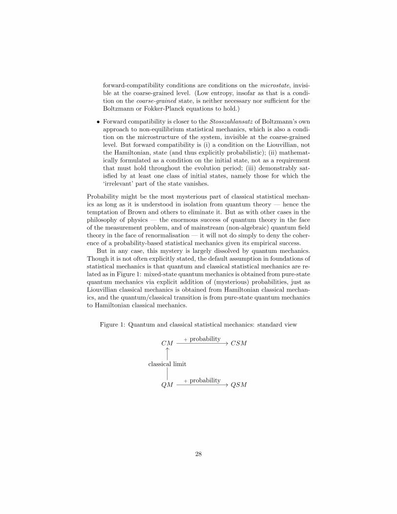
But in any case, this mystery is largely dissolved by quantum mechanics.Though it is not often explicitly stated, the default assumption in foundations ofstatistical mechanics is that quantum and classical statistical mechanics are re-lated as in Figure 1: mixed-state quantum mechanics is obtained from pure-statequantum mechanics via explicit addition of (mysterious) probabilities, just asLiouvillian classical mechanics is obtained from Hamiltonian classical mechan-ics, and the quantum/classical transition is from pure-state quantum mechanicsto Hamiltonian classical mechanics.

Figure 1: Quantum and classical statistical mechanics: standard view

CM CSM

QM QSM

+ probability

classical limit

+ probability

28

We have seen that this is not viable:

• The analogy between pure/mixed states and Hamiltonian/Liouvillian statesis superficial: mixed states are already required as part of the formalismof quantum mechanics by subsystem considerations (section 7) and theaddition of mysterious additional probabilities does not therefore gener-alise the dynamics in the quantum case as it does in the classical. Anyequation of quantum mechanics in which probability distributions over(pure or mixed) states can always be reinterpreted as an equation aboutindividual mixed states, so there is no inference from the empirical successof a given part of quantum statistical mechanics to the need for statistical-mechanical probabilities.

• Study of the quantum-classical transition shows that quantum states (pureor mixed) correspond to phase-space distributions, not to phase-spacepoints, and so argues for an understanding of that transition as a tran-sition from quantum mechanics to Liouvillian, not Hamiltonian, classicalmechanics.

• Elementary considerations of wave-packet spreading, applied to dilute-gassystems with realistic parameters, reveals that Hamiltonian mechanicscompletely fails for such systems: inter-particle collisions are more likeplane-wave interactions than classical hard-sphere scattering, and leadrapidly to a highly entangled state. So interpretation of the Boltzmannequation as a one-particle-marginal probability distribution (or relative-frequency description of) the trajectories of well-localised, deterministi-cally evolving point particles is unjustified in our quantum universe. Onthe other hand, the derivation of that equation from Liouvillian dynam-ics via the BBGKY hierarchy remains valid even when the Liouvilliandynamics are understood as an approximate description of Schrodingerdynamics, and indeed can be replicated exactly, mutatis mutandis, in theWigner-function formalism.

• In a stochastic dynamics like the Brownian motion described by the Langevinequation, once we consider it quantum-mechanically we find that thestochasticity is itself quantum-mechanical, and persists even if the sys-tem and its environment begins in a pure state.

There is, in short, abundant evidence that ‘statistical-mechanical’ probabilitiesare just quantum-mechanical probabilities. Considerations of the structure ofquantum theory, of phase-space descriptions of quantum mechanics, and of spe-cific models, all tell us that Liouvillian states need to be understood as quantumstates in the regime where the Liouville equation approximates the Schrodingerequation, and not as application of a new notion of probability to Hamiltoniandynamics. Hamiltonian dynamics is an approximation to Liouvillian dynamicsin certain regimes, not its underpinning.8 The correct relation between classical

8Of course, this is entirely compatible with the use of Hamiltonian dynamics as a formalmethod to analyse Liouvillian dynamics.

29

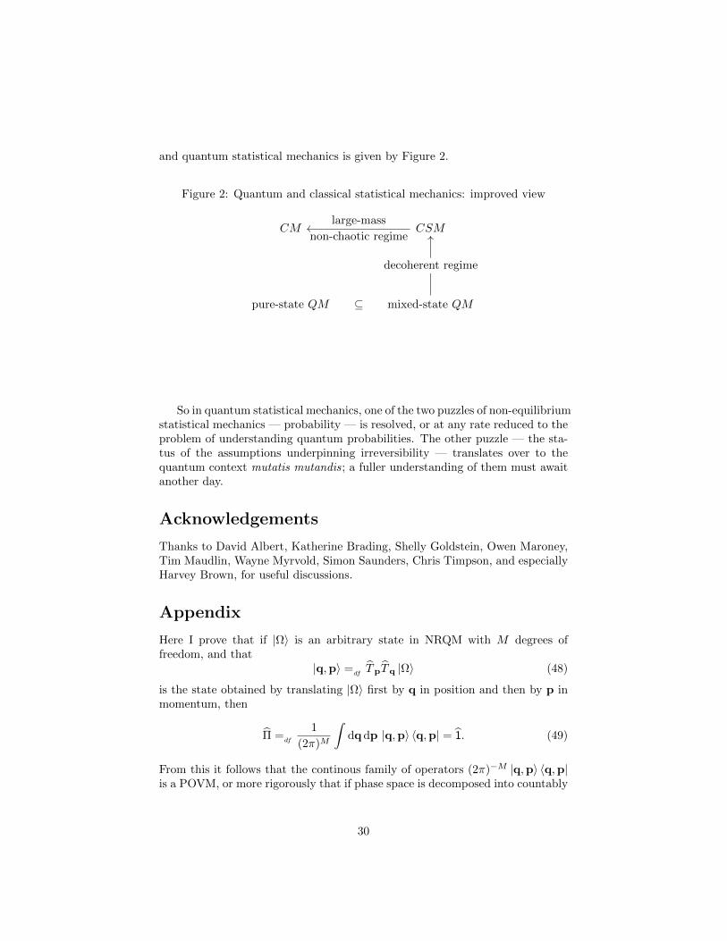
and quantum statistical mechanics is given by Figure 2.

Figure 2: Quantum and classical statistical mechanics: improved view

CM CSM

pure-state QM mixed-state QM

large-mass

non-chaotic regime

⊆

decoherent regime

So in quantum statistical mechanics, one of the two puzzles of non-equilibriumstatistical mechanics — probability — is resolved, or at any rate reduced to theproblem of understanding quantum probabilities. The other puzzle — the sta-tus of the assumptions underpinning irreversibility — translates over to thequantum context mutatis mutandis; a fuller understanding of them must awaitanother day.

Acknowledgements

Thanks to David Albert, Katherine Brading, Shelly Goldstein, Owen Maroney,Tim Maudlin, Wayne Myrvold, Simon Saunders, Chris Timpson, and especiallyHarvey Brown, for useful discussions.

Appendix

Here I prove that if |Ω〉 is an arbitrary state in NRQM with M degrees offreedom, and that

|q,p〉 =dfTpTq |Ω〉 (48)

is the state obtained by translating |Ω〉 first by q in position and then by p inmomentum, then

Π =df

1

(2π)M

∫dq dp |q,p〉 〈q,p| = 1. (49)

From this it follows that the continous family of operators (2π)−M |q,p〉 〈q,p|is a POVM, or more rigorously that if phase space is decomposed into countably

30

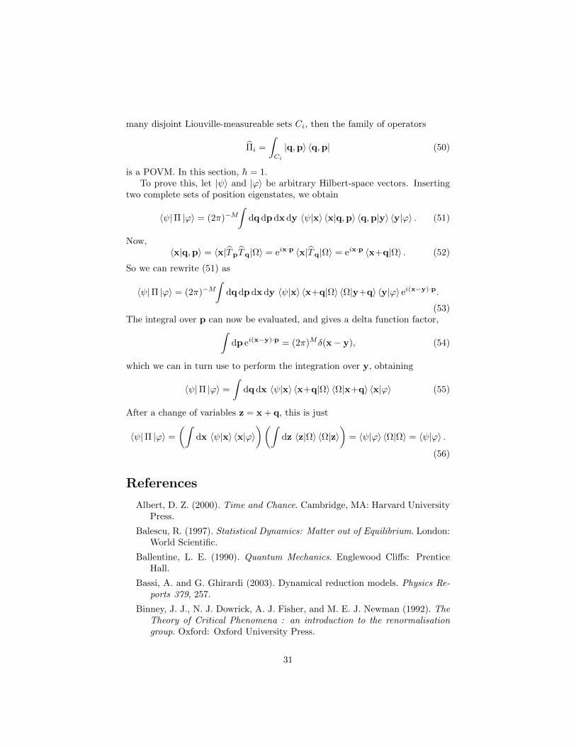
many disjoint Liouville-measureable sets Ci, then the family of operators

Πi =

∫Ci

|q,p〉 〈q,p| (50)

is a POVM. In this section, h = 1.To prove this, let |ψ〉 and |ϕ〉 be arbitrary Hilbert-space vectors. Inserting

two complete sets of position eigenstates, we obtain

〈ψ|Π |ϕ〉 = (2π)−M∫

dq dp dx dy 〈ψ|x〉 〈x|q,p〉 〈q,p|y〉 〈y|ϕ〉 . (51)

Now,〈x|q,p〉 = 〈x|TpTq|Ω〉 = eix·p 〈x|Tq|Ω〉 = eix·p 〈x+q|Ω〉 . (52)

So we can rewrite (51) as

〈ψ|Π |ϕ〉 = (2π)−M∫

dq dp dx dy 〈ψ|x〉 〈x+q|Ω〉 〈Ω|y+q〉 〈y|ϕ〉 ei(x−y)·p.

(53)The integral over p can now be evaluated, and gives a delta function factor,∫

dp ei(x−y)·p = (2π)Mδ(x− y), (54)

which we can in turn use to perform the integration over y, obtaining

〈ψ|Π |ϕ〉 =

∫dq dx 〈ψ|x〉 〈x+q|Ω〉 〈Ω|x+q〉 〈x|ϕ〉 (55)

After a change of variables z = x + q, this is just

〈ψ|Π |ϕ〉 =

(∫dx 〈ψ|x〉 〈x|ϕ〉

)(∫dz 〈z|Ω〉 〈Ω|z〉

)= 〈ψ|ϕ〉 〈Ω|Ω〉 = 〈ψ|ϕ〉 .

(56)

References

Albert, D. Z. (2000). Time and Chance. Cambridge, MA: Harvard UniversityPress.

Balescu, R. (1997). Statistical Dynamics: Matter out of Equilibrium. London:World Scientific.

Ballentine, L. E. (1990). Quantum Mechanics. Englewood Cliffs: PrenticeHall.

Bassi, A. and G. Ghirardi (2003). Dynamical reduction models. Physics Re-ports 379, 257.

Binney, J. J., N. J. Dowrick, A. J. Fisher, and M. E. J. Newman (1992). TheTheory of Critical Phenomena : an introduction to the renormalisationgroup. Oxford: Oxford University Press.

31

Bohm, D. (1952). A Suggested Interpretation of Quantum Theory in Termsof “Hidden” Variables. Physical Review 85, 166–193.

Bohm, D. and B. J. Hiley (1993). The Undivided Universe: An OntologicalInterpretation of Quantum Theory. London: Routledge and Kegan Paul.

Brown, H. R., W. Myrvold, and J. Uffink (2009). Boltzmann’s H-theorem, itsdiscontents, and the birth of statistical mechanics. Studies in History andPhilosophy of Modern Physics 40, 174–191.

Cartwright, N. (1983). How the Laws of Physics Lie. Oxford: Oxford Univer-sity Press.

Cartwright, N. (1999). The Dappled World: A Study of the Boundaries ofScience. Cambridge: Cambridge University Press.

DeWitt, B. and N. Graham (Eds.) (1973). The many-worlds interpretation ofquantum mechanics. Princeton: Princeton University Press.

Durr, D., S. Goldstein, and N. Zanghi (1996). Bohmian mechanics as the foun-dation of quantum mechanics. In J. T. Cushing, A. Fine, and S. Goldstein(Eds.), Bohmian Mechanics and Quantum Theory: An Appraisal, pp. 21–44. Dordrecht: Kluwer Academic Publishers.

Everett, H. I. (1957). Relative State Formulation of Quantum Mechanics.Review of Modern Physics 29, 454–462. Reprinted in DeWitt and Graham(1973).

Ghirardi, G., A. Rimini, and T. Weber (1986). Unified Dynamics for Microand Macro Systems. Physical Review D 34, 470–491.

Goldstein, S., J. L. Lebowitz, R. Tumulka, and N. Zanghi (2006). Canonicaltypicality. Physical Review Letters 96, 050403.

Hudson, R. (1974). When is the Wigner quasi-probability density non-negative? Reports on Mathematical Physics 6, 249–252.

Lanford, O. (1975). Time evolution of large classical systems. In J. Moser(Ed.), Dynamical Systems, Theory and Applications, pp. 1–111. Berlin:Springer.

Lanford, O. (1976). On the derivation of the Boltzmann equation. Aster-isque 40, 117–137.

Liboff, R. L. (2003). Kinetic Theory: Classical, Quantum and RelativisticDescriptions (Third ed.). New York: Springer-Verlag.

Malabarba, A. S. L., L. P. Garcia-Pintos, N. Linden, T. C. Farrelly, and A. J.Short (2014). Quantum systems equilibrate rapidly for most observables.Physical Review E 90, 012121.

Paz, J. and W. Zurek (2002). Environment-induced decoherence and the tran-sition from quantum to classical. Lectures given by both authors at the72nd Les Houches Summer School on “Coherent Matter Waves”, July-August 1999. Available online at arxiv.org/abs/quant-ph/0010011.

32

Pearle, P. (1989). Combining Stochastic Dynamical State-Vector Reductionwith Spontaneous Localization. Physical Review A 39 (5), 2277–2289.

Peres, A. (1993). Quantum Theory: Concepts and Methods. Dordrecht:Kluwer Academic Publishers.

Short, A. J. (2011). Equilibration of quantum systems and subsystems. NewJournal of Physics 13, 053009.

Sklar, L. (1993). Physics and Chance: Philosophical Issues in the Foundationsof Statistical Mechanics. Cambridge: Cambridge University Press.

Tolman, R. C. (1938). The principles of statistical mechanics. Oxford Univer-sity P.

Uffink, J. and G. Valente (2015). Lanford’s theorem and the emergence ofirreversibility. Foundations of Physics 45, 404–438.

Valente, G. (2014). The approach towards equilibrium in Lanfords theorem.European Journal for the Philosophy of Science 4, 309–335.

Wallace, D. (2010). The logic of the past hypothesis. Available online athttp://users.ox.ac.uk/ mert0130/papers.shtml.

Wallace, D. (2012). The Emergent Multiverse: Quantum Theory according tothe Everett Interpretation. Oxford: Oxford University Press.

Wallace, D. (2016). What is orthodox quantum mechanics? available onlineat https://arxiv.org/abs/1604.05973.

Zeh, H. D. (2007). The Physical Basis of the Direction of Time (5th ed.).Berlin: Springer.

Zurek, W. and J. P. Paz (1995). Quantum chaos: a decoherent definition.Physica D 83, 300–308.

Zwanzig, R. (1960). Ensemble method in the theory of irreversibility. Journalof Chemical Physics 33, 1338–1341.

Zwanzig, R. (1966). Statistical mechanics of irreversibility. In P. H. E. Meijer(Ed.), Quantum Statistical Mechanics, pp. 139. New York: Gordon andBreach.

Zwanzig, R. (2001). Nonequilibrium Statistical Mechanics. Oxford: OxfordUniversity Press.

33