Probability - University of Tennessee at Chattanooga · Web viewExample: Statistics taught with lab vs. Statistics taught without lab. Question: Is the mean amount learned by the

Lecture 6

Hypothesis Testing and One Population TestsHowell Ch 8, 12

Statistical Inference - Using sample data to make statements about population characteristics.

Two basic processes

I. Estimation of the value of a population parameter.

Question asked: What is the value of the population parameter?

Answer: A number, called a point estimate, or an interval, called a confidence interval. The interval is one that has a prespecified probability (usually .95) of surrounding the population parameter.

Example: What % of persons think we should bomb selected targets in Syria?

A typical answer would have the form: 38% with a 5% margin of error.

This is a combination of point estimate (the 38%) and an interval estimate (from 38-5 to 38+5 or from 33 to 43%). The 5% means that the interval has probability 100 – 5% = 95% of surrounding the true population percentage. From this we could conclude that it’s quite likely that the majority population does NOT want strikes.

II. Hypothesis Testing. Null Hypothesis Significance Testing (NHST)

A. With one population.

Deciding whether a particular population parameter (usually the mean) equals a value specified by prior research or other considerations.

Example: A light bulb is advertised as having an “average lifetime” of 5000 hours.

Question: Is the mean of the population of lifetimes of bulbs produced by the manufacturer equal to 5000 or not?

B. With two populations.

Deciding whether corresponding parameters (usually means) of the two populations are equal or not.

Example: Statistics taught with lab vs. Statistics taught without lab.

Question: Is the mean amount learned by the population of students taught with a lab equal to the mean amount learned by the population of students taught without lab?

C. Three populations.

Deciding whether corresponding parameters (usually means) of the three populations are equal or not. And on and on and on.

Inference and One Population Tests - 1 5/8/2023

Introduction to Hypothesis Testing Start here on 10/10/17.

Suppose we have a single population, say the population of light bulbs mentioned above.

Suppose we want to determine whether or not the mean of the population equals 5000.

Two possibilities

0. The population mean equals 5000, i.e., it is not different from 5000.1. The population mean does not equal 5000, i.e., it is different from 5000.

These possibilities are called hypotheses.

The first, the hypothesis of no difference is called the Null Hypothesis: H0.

The second, the hypothesis of a difference is called the Alternative Hypothesis: H1.

Our task is to decide which of the two hypotheses is true.

Two general approaches

1. The Bill Gates (Warren Buffet, Carlos Slim Helu’) approach.

Purchase ALL the light bulbs in the population. Measure the lifetime of each bulb. Compute the mean. If the mean equals 5000, retain the null. If the mean does not equal 5000, reject the null.Problem: Too many bulbs. Cost would be enormous. Might not even be possible to get all of them.

2. The Plan B approach.

Take a sample of light bulbs.

Compute the mean of the sample.

Apply the following, intuitively reasonable decision rule

If the value of the sample mean is “close” to 5000, decide that the null must be true.If the value of the sample mean is “far” from 5000, decide that the null must be false.

But how close is “close”? How far is “far”?

What if the mean of the lifetimes of 25 bulbs were 4999.99?



Clearly we need some rules.


The p-value.

Statisticians have decided to redefine “close” and “far” in terms of probabilities.

They first compute the probability of an outcome as extreme as the sample outcome if the null were true. That probability is called the p-value for the experiment.

The p-value is also called the probability of the obtained outcome due to chance alone.

The significance level.

Statisticians then choose a criterion or cutoff representing the dividing line between p-values that are small and p-values that are large. That value is called the significance level of the statistical test. It is typically .05 or some value smaller than .05.

They then use the following rule:

Loosely . . .

If the p-value is less than or equal to the significance level, then reject the null hypothesis

If the probability of the observed outcome due to chance alone is small, then it must not be due to chance, so reject the null (chance) hypothesis.

Suppose the mean lifetime of 25 bulbs was only 672.6 hours.

You might think, “Gosh, if the population mean were 5000, then most of the bulbs in the sample would have lasted around 5000 hours, so the sample mean would be pretty close to 5000. The probably of getting a sample mean of only 672.6 would be very small. So, I’ll reject the null hypothesis.”

If the p-value is larger than the significance level, then retain the null hypothesis.

If the probability of the observed outcome due to chance along is large, then it must be due to chance, so retain the null (chance) hypothesis.

Suppose the mean lifetime of 25 bulbs was 4993.4.

You might think, “Gosh, if the population mean were 5000, then most of the bulbs in the sample would have lasted around 5000, so the probability of getting a sample mean that close to 5000 would be pretty large. So, I’ll retain the null hypothesis.”

To summarize:

If the p-value is less than or equal to the significance level, then reject the null.

If the p-value is larger than the significance level, then retain the null.


The Steps in Hypothesis Testing

Step 1. From the problem description, state the null hypothesis required by the problem and the alternative hypothesis.

Step 2. Choose a test statistic whose value will allow you to decide between the null and the alternative hypothesis.

Step 3. Determine the sampling distribution of that test statistic under the assumption that the null hypothesis is true. We need the sampling distribution in order to get the p-value. The good news is that most test statistics follow one of four sampling distributions – Normal, T, F, and Chi-square.

Once you've determined the sampling distribution, you'll know what values of the test statistic would be expected to occur if the null were true and what values would not be expected if the null were true.

Step 4. Set the significance level of the test.

Step 5. Compute the value of the test statistic.

Step 6. Compute the p-value of the test statistic.

The p-value is the probability of a value as extreme as the obtained value if the null were true, i.e., the probability of the obtained outcome due only to chance. In most cases, it will be printed by SPSS. Unfortunately, it will be labeled "Sig." not p.

Step 7. Compare the p-value with the significance level and make your decision.

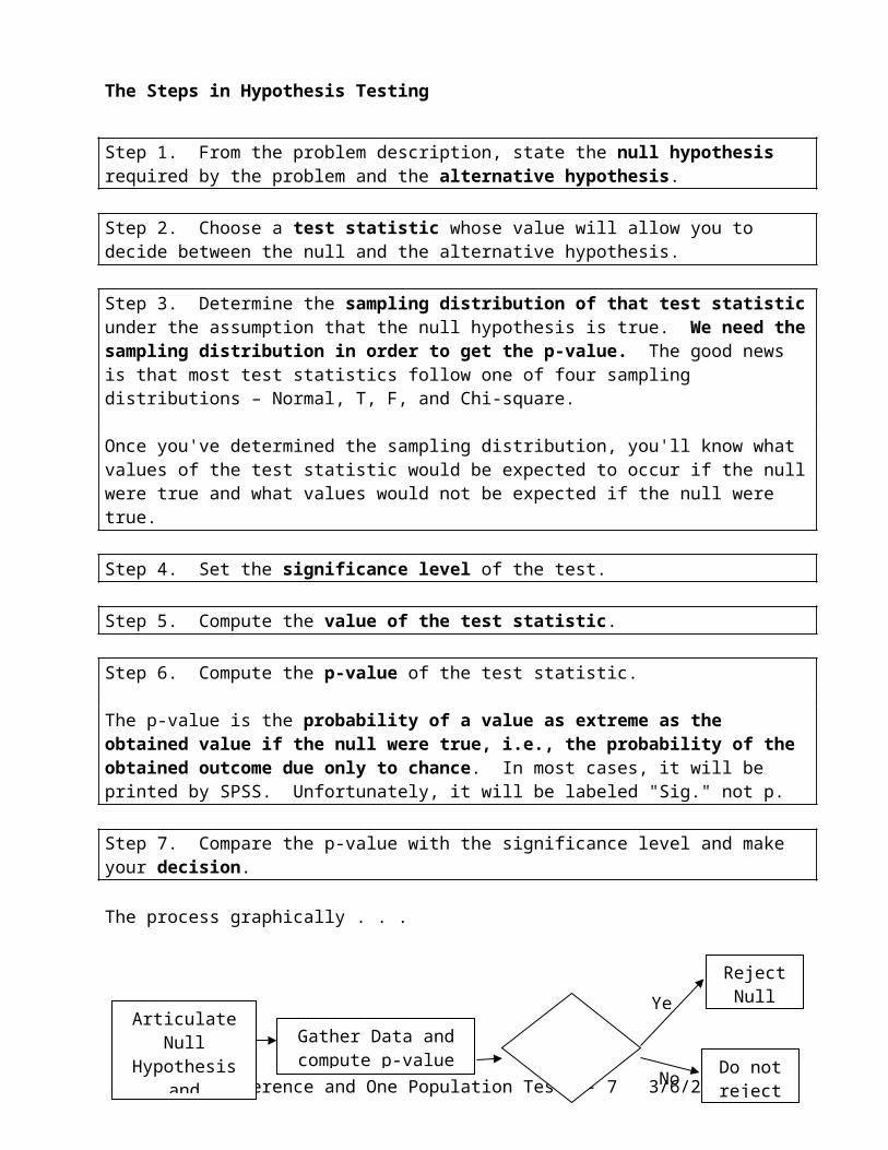
The process graphically . . .


Articulate Null Hypothesis and

Alternative Hypothesis

Gather Data and compute p-value Do not

reject Null

p < = Significance

level? No

Reject NullYes

Worked Out Example

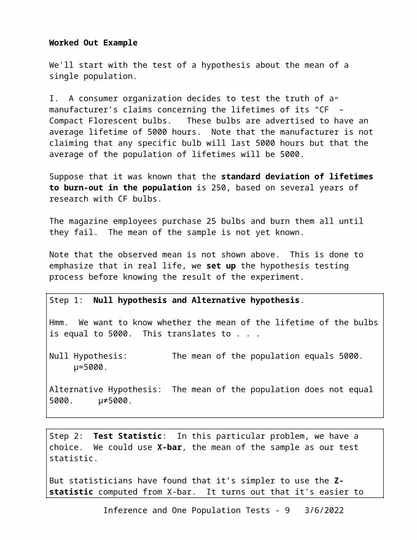
We'll start with the test of a hypothesis about the mean of a single population.

I. A consumer organization decides to test the truth of a manufacturer’s claims concerning the lifetimes of its “CF” – Compact Florescent bulbs. These bulbs are advertised to have an average lifetime of 5000 hours. Note that the manufacturer is not claiming that any specific bulb will last 5000 hours but that the average of the population of lifetimes will be 5000.

Suppose that it was known that the standard deviation of lifetimes to burn-out in the population is 250, based on several years of research with CF bulbs.

The magazine employees purchase 25 bulbs and burn them all until they fail. The mean of the sample is not yet known.

Note that the observed mean is not shown above. This is done to emphasize that in real life, we set up the hypothesis testing process before knowing the result of the experiment.

Step 1: Null hypothesis and Alternative hypothesis.

Hmm. We want to know whether the mean of the lifetime of the bulbs is equal to 5000. This translates to . . .

Null Hypothesis: The mean of the population equals 5000. µ=5000.

Alternative Hypothesis: The mean of the population does not equal 5000. µ≠5000.

Step 2: Test Statistic: In this particular problem, we have a choice. We could use X-bar, the mean of the sample as our test statistic.

But statisticians have found that it’s simpler to use the Z-statistic computed from X-bar. It turns out that it's easier to use the Z-statistic from the start, since we ultimately have to compute it anyway.


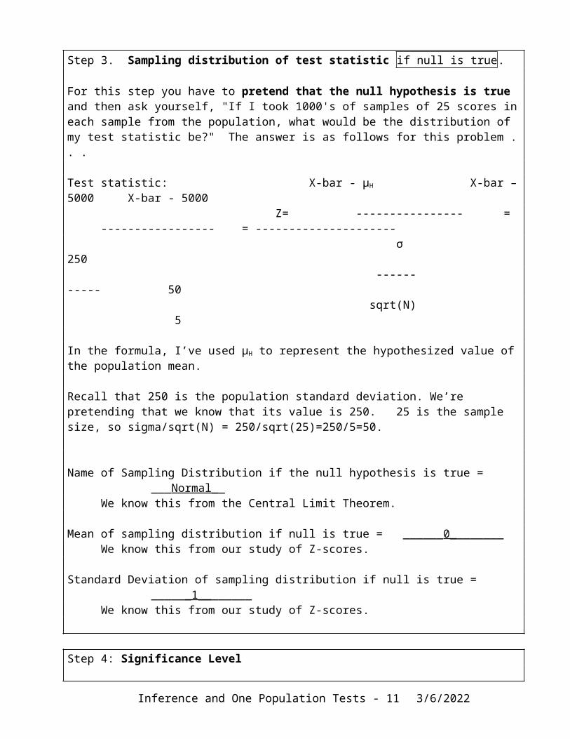
Step 3. Sampling distribution of test statistic if null is true.

For this step you have to pretend that the null hypothesis is true and then ask yourself, "If I took 1000's of samples of 25 scores in each sample from the population, what would be the distribution of my test statistic be?" The answer is as follows for this problem . . .

Test statistic: X-bar - µH X-bar – 5000 X-bar - 5000 Z= ---------------- = ----------------- = --------------------- σ 250 ------ ----- 50 sqrt(N) 5

In the formula, I’ve used µH to represent the hypothesized value of the population mean.

Recall that 250 is the population standard deviation. We’re pretending that we know that its value is 250. 25 is the sample size, so sigma/sqrt(N) = 250/sqrt(25)=250/5=50.

Name of Sampling Distribution if the null hypothesis is true = ___Normal__We know this from the Central Limit Theorem.

Mean of sampling distribution if null is true = ______0________We know this from our study of Z-scores.

Standard Deviation of sampling distribution if null is true = ______1________We know this from our study of Z-scores.

Step 4: Significance Level

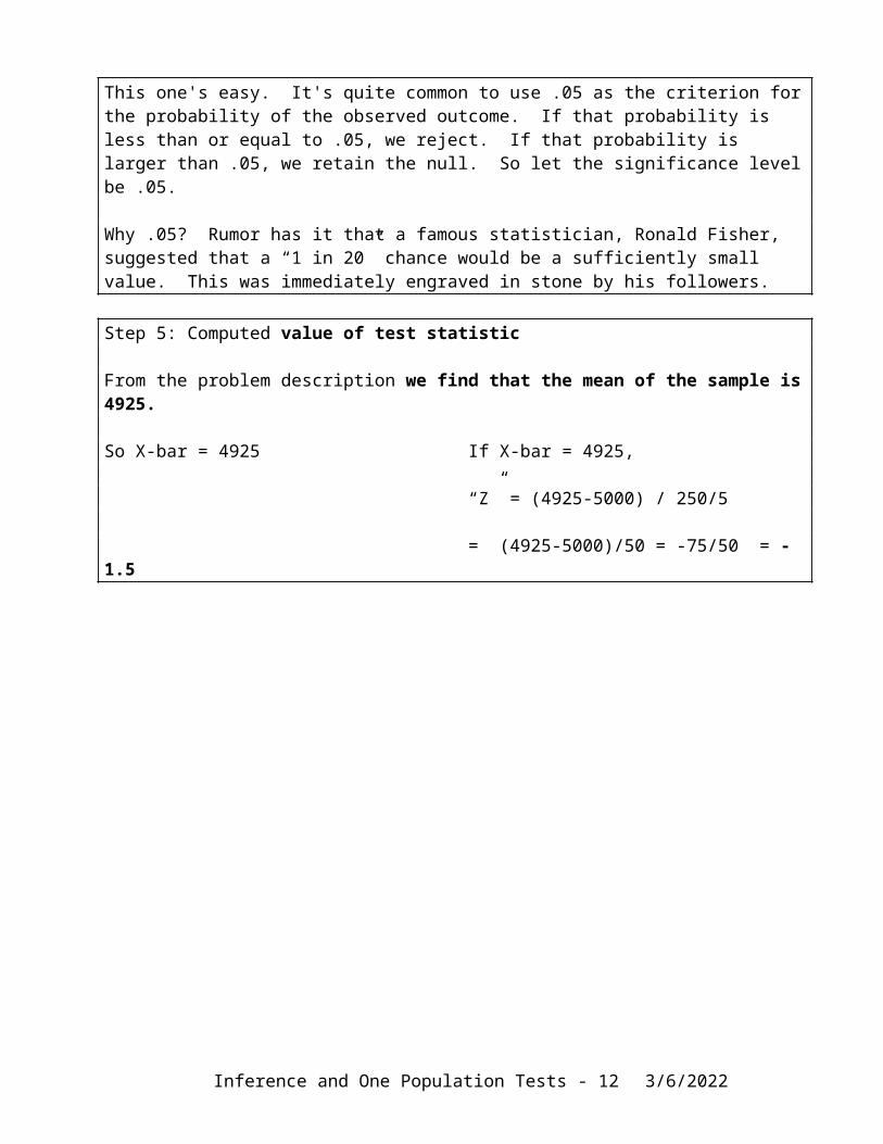
This one's easy. It's quite common to use .05 as the criterion for the probability of the observed outcome. If that probability is less than or equal to .05, we reject. If that probability is larger than .05, we retain the null. So let the significance level be .05.

Why .05? Rumor has it that a famous statistician, Ronald Fisher, suggested that a “1 in 20” chance would be a sufficiently small value. This was immediately engraved in stone by his followers.

Step 5: Computed value of test statistic

From the problem description we find that the mean of the sample is 4925.

So X-bar = 4925 If X-bar = 4925,

“Z” = (4925-5000) / 250/5

= (4925-5000)/50 = -75/50 = -1.5


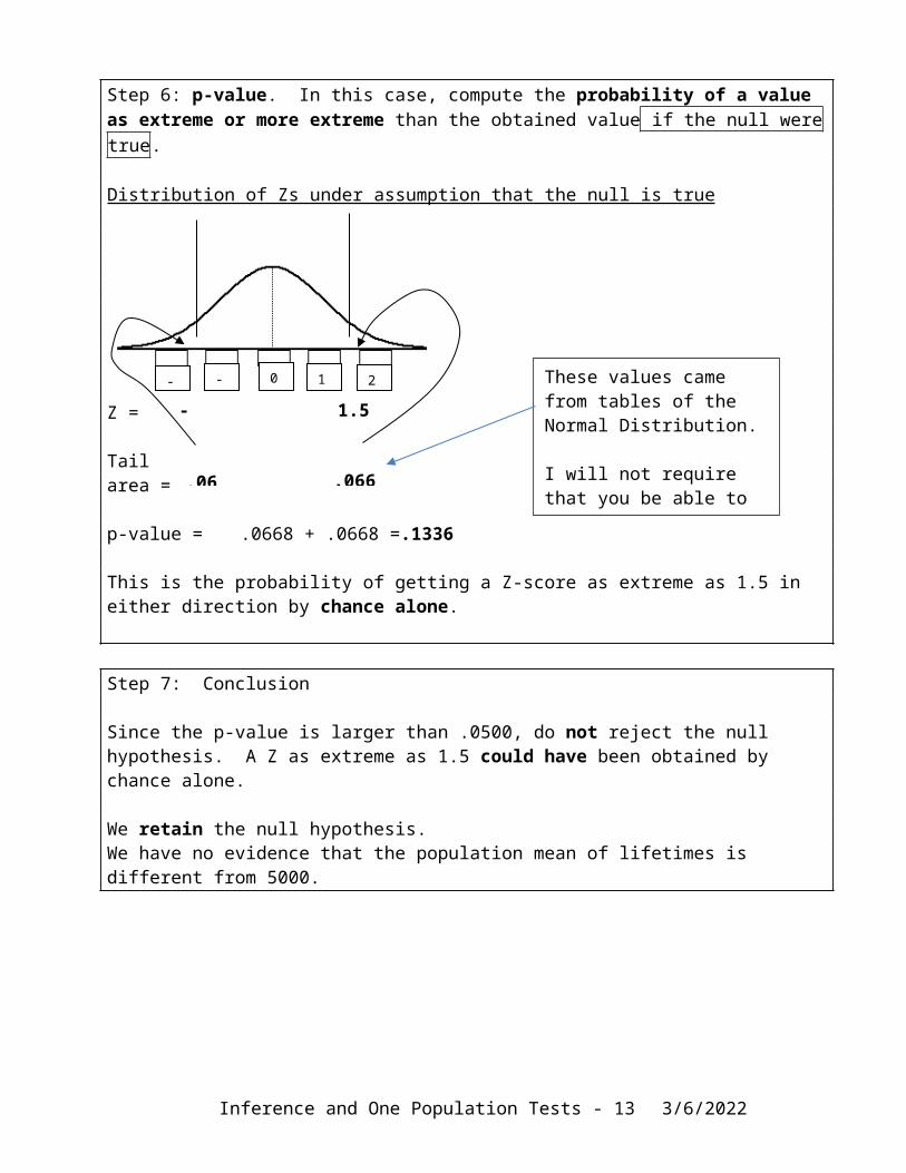
Step 6: p-value. In this case, compute the probability of a value as extreme or more extreme than the obtained value if the null were true.

Distribution of Zs under assumption that the null is true

Z =

Tail area =

p-value = .0668 + .0668 =.1336

This is the probability of getting a Z-score as extreme as 1.5 in either direction by chance alone.

Step 7: Conclusion

Since the p-value is larger than .0500, do not reject the null hypothesis. A Z as extreme as 1.5 could have been obtained by chance alone.

We retain the null hypothesis.We have no evidence that the population mean of lifetimes is different from 5000.


0 1 2-1-2

.0668 .0668

-1.5 1.5

0 1 2-1-2 These values came from tables of the Normal Distribution.

I will not require that you be able to do this calculation by hand. We’ll get the p-value from computer output.

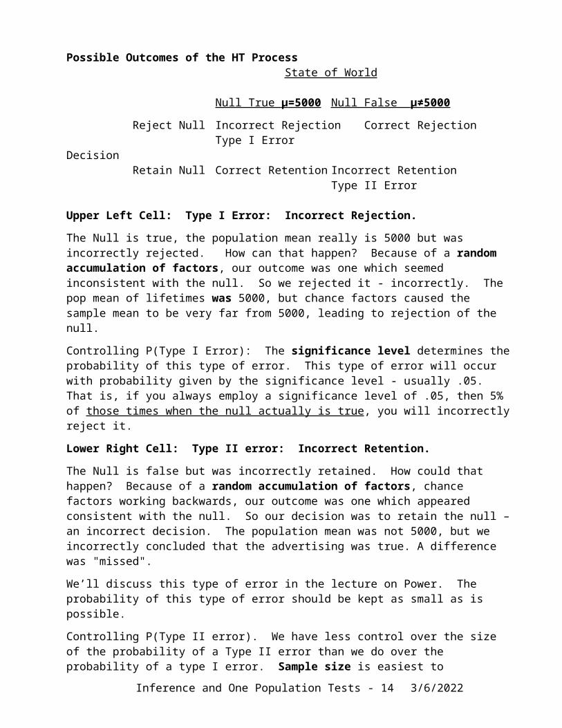
Possible Outcomes of the HT Process State of World

Null True µ =5000 Null False µ≠ 5000

Reject Null Incorrect Rejection Correct RejectionType I Error

DecisionRetain Null Correct Retention Incorrect Retention

Type II Error

Upper Left Cell: Type I Error: Incorrect Rejection.

The Null is true, the population mean really is 5000 but was incorrectly rejected. How can that happen? Because of a random accumulation of factors, our outcome was one which seemed inconsistent with the null. So we rejected it - incorrectly. The pop mean of lifetimes was 5000, but chance factors caused the sample mean to be very far from 5000, leading to rejection of the null.

Controlling P(Type I Error): The significance level determines the probability of this type of error. This type of error will occur with probability given by the significance level - usually .05. That is, if you always employ a significance level of .05, then 5% of those times when the null actually is true, you will incorrectly reject it.

Lower Right Cell: Type II error: Incorrect Retention.

The Null is false but was incorrectly retained. How could that happen? Because of a random accumulation of factors, chance factors working backwards, our outcome was one which appeared consistent with the null. So our decision was to retain the null – an incorrect decision. The population mean was not 5000, but we incorrectly concluded that the advertising was true. A difference was "missed".

We’ll discuss this type of error in the lecture on Power. The probability of this type of error should be kept as small as is possible.

Controlling P(Type II error). We have less control over the size of the probability of a Type II error than we do over the probability of a type I error. Sample size is easiest to manipulate. Larger sample sizes lead to smaller P(Type II error). More on this in the section on Power.

Lower Left Cell: Correct Retention: Retaining a true null hypothesis. The null is true. It should have been retained and it was. This is affirming the null. It is a correct decision. The manufacturer’s claim was correct, and we concluded that it was correct.

Controlling: Significance level.

Upper Right Cell: Correct Rejection: Rejecting a false null hypothesis

The null is false. It should have been rejected, and it was. This is where we want to be. The null was false. We "detected" the difference. The manufacturer’s claim was not correct, and we detected that it was not correct.

The probability of correctly rejecting a false Null is called the Power of the statistical test. Power equals 1 - P(Type II Error). More on power later.

Controlling: Same factors as those that affect P(Type II error). Sample size is most frequently employed.


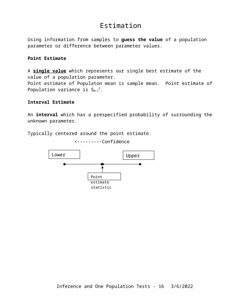
Estimation

Using information from samples to guess the value of a population parameter or difference between parameter values.

Point Estimate

A single value which represents our single best estimate of the value of a population parameter.Point estimate of Populaton mean is sample mean. Point estimate of Population variance is SN-1

2.

Interval Estimate

An interval which has a prespecified probability of surrounding the unknown parameter.

Typically centered around the point estimate.

Both point estimates and confidence intervals are computed and printed by our statistical packages.

Statistics used as point estimates: Sample mean, Difference between two sample means, Pearson r

Estimation related to Hypothesis Testing

A statistical law that relates estimation to hypothesis testing is the following:

If you have a 95% confidence interval for a population parameter,

1) ANY value outside the confidence interval would be a “rejection” at significance level = .05.

2) ANY value within the confidence interval would be a “retention” at significance level = .05.

Suppose the 95% confidence interval for the light bulb problem is 4827 – 5023.

Since this interval includes 5000, this means that our sample mean of 4925 in the above problem would be a retention value.

On the other hand, if the sample mean had been 4825, that value would result in a rejection of the null.


Point estimate

Lower limit Upper limit

<---------Confidence Interval---------->

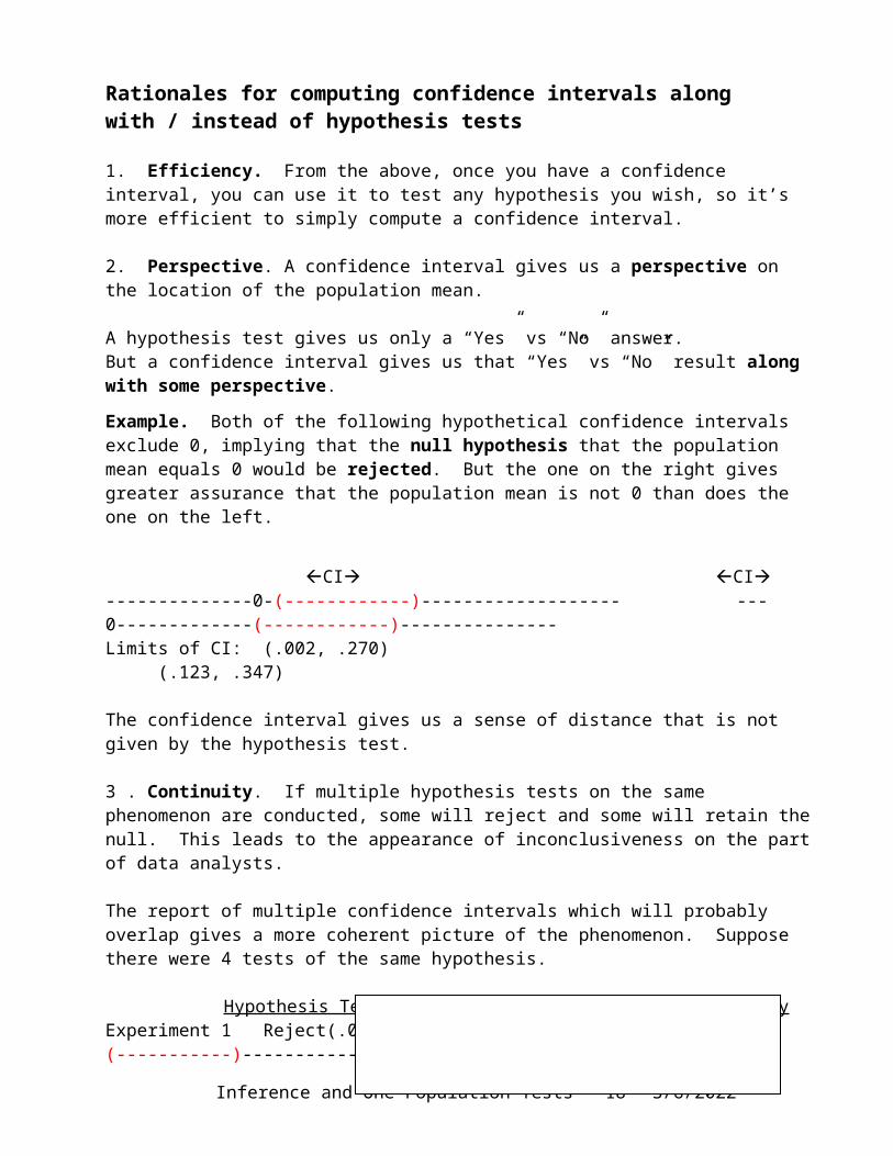
Rationales for computing confidence intervals along with / instead of hypothesis tests

1. Efficiency. From the above, once you have a confidence interval, you can use it to test any hypothesis you wish, so it’s more efficient to simply compute a confidence interval.

2. Perspective. A confidence interval gives us a perspective on the location of the population mean.

A hypothesis test gives us only a “Yes” vs “No” answer. But a confidence interval gives us that “Yes” vs “No” result along with some perspective.

Example. Both of the following hypothetical confidence intervals exclude 0, implying that the null hypothesis that the population mean equals 0 would be rejected. But the one on the right gives greater assurance that the population mean is not 0 than does the one on the left.

CI CI--------------0-(------------)------------------- ---0-------------(------------)---------------Limits of CI: (.002, .270) (.123, .347)

The confidence interval gives us a sense of distance that is not given by the hypothesis test.

3 . Continuity. If multiple hypothesis tests on the same phenomenon are conducted, some will reject and some will retain the null. This leads to the appearance of inconclusiveness on the part of data analysts.

The report of multiple confidence intervals which will probably overlap gives a more coherent picture of the phenomenon. Suppose there were 4 tests of the same hypothesis.

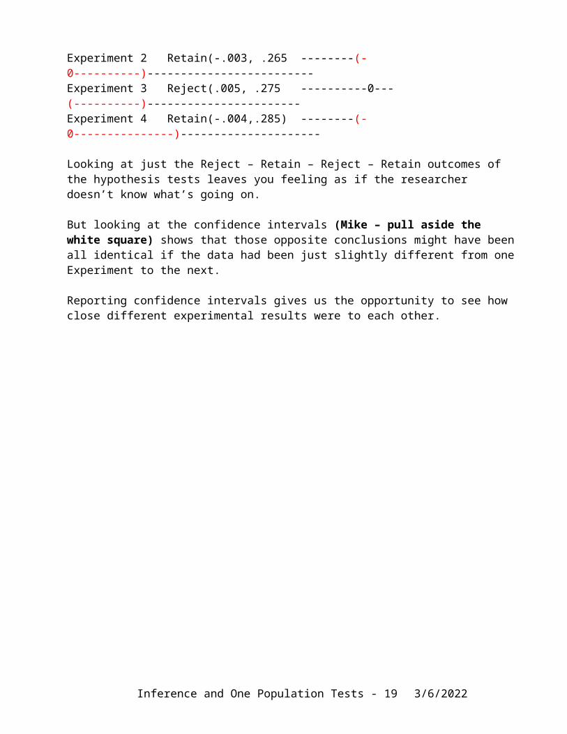
Hypothesis Tests CIs CIs GraphicallyExperiment 1 Reject (.002, .270 ----------0-(-----------)-----------------------Experiment 2 Retain (-.003, .265 --------(-0----------)-------------------------Experiment 3 Reject (.005, .275 ----------0---(----------)-----------------------Experiment 4 Retain (-.004, .285) --------(-0---------------)---------------------

Looking at just the Reject – Retain – Reject – Retain outcomes of the hypothesis tests leaves you feeling as if the researcher doesn’t know what’s going on.

But looking at the confidence intervals (Mike – pull aside the white square) shows that those opposite conclusions might have been all identical if the data had been just slightly different from one Experiment to the next.

Reporting confidence intervals gives us the opportunity to see how close different experimental results were to each other.


Example involving One Population Mean - value of sigma not knownA manufacturer of tires claims that average lifetime of its tires is 30,000 miles. A sample of 25 tires is purchased and the tires are put on test cars that are driven until the tire tread reaches the minimum legal depth. Based on the results of the sample, what can be concluded about the manufacturer's claim? Suppose that you don’t know the value of the population standard deviation. Suppose that the mean of the sample of 25 tires was 29,640 with sample standard deviation equal to 900.

Step 1. From the problem description, state the null hypothesis required by the problem and the alternative hypothesis.

Null: Mean of the population of mileages of the tires is 30,000.Alternative: Mean of the population of mileages is not 30,000.

Step 2. Choose a test statistic whose value will allow you to decide between the null and the alternative hypothesis.

We can’t use the Z statistic, because its formula requires that we know the value of the population standard deviation.

A natural substitution for the population standard deviation is the sample standard deviation.

This would yield the formula, (X-bar – 30,000)Statistic = --------------------------------- Sample SD / square root of N

Step 3. Determine the sampling distribution of that test statistic under the assumption that the null hypothesis is true.

The statistic above is NOT a Z, since S, rather than sigma has been used in the denominator.

So the sampling distribution is not the Normal Distribution, as it would be if the statistic were Z.

The actual formula for the sampling distribution was discovered by William Gossett, in the early 1900’s.

He called the statistic the t statistic and called the distribution the T distribution.

The T distribution has mean 0. Its standard deviation is larger than 1, and depends on a quantity called degrees of freedom.In the one-sample case, df = N – 1 = 24 for our example.

The shape of the T distribution is similar to the Normal.

Step 4. Set the significance level of the test. We’ll use .05.

Step 5. Compute the value of the test statistic.

Since the sample mean is 29,640,

t = (29,640 – 30,000) / (900/5) = 360/180 = -2.00.


Step 6. Compute the p-value of the test statistic.

The p-value is the probability of a t as extreme as -2.00.

The formula for computing the p-value for a t is quite complicated. Luckily, we have computers.Our computer program will compute the value of t and its p-value automatically. That p is .057, as shown on the next page.

Or we could look up the critical t for df = 24 and alpha = .05. That critical t value, from the text, is 2.064.

If the obtained t exceeds the critical t in absolute value that would mean that p would be less than or equal to .05 and we could reject the null.

Step 7. Compare the p-value with the significance level and make your decision.

Since p > .05, do not reject the null hypothesis that Population mean = 30,000. We will act as if the population mean is equal to 30,000.

So, we rejected the null hypothesis when using the Z statistic.But we did not reject the null when using the t.This illustrates the fact that the Z statistic is slightly more powerful than the t.


One Sample t – SPSS ExampleA manufacturer of tires claims that average lifetime of its tires is 30,000 miles. A sample of 25 tires is purchased and the tires are put on test cars that are driven until the tire tread reaches the minimum legal depth. Based on the results of the sample, what can be concluded about the manufacturer's claim? The mileage values for the tires are below.

id mileage

1 29050 2 29837 3 29622 4 29546 5 28197 6 28277

7 29585 8 31344 9 29702 10 29585 11 29564 12 28824

13 31158 14 29084 15 29467 16 28261 17 28496 18 30784

19 30534 20 30397 21 29883 22 29077 23 31239 24 29630 25 29857

Mike – show how to put the data from this Word doc into SPSS


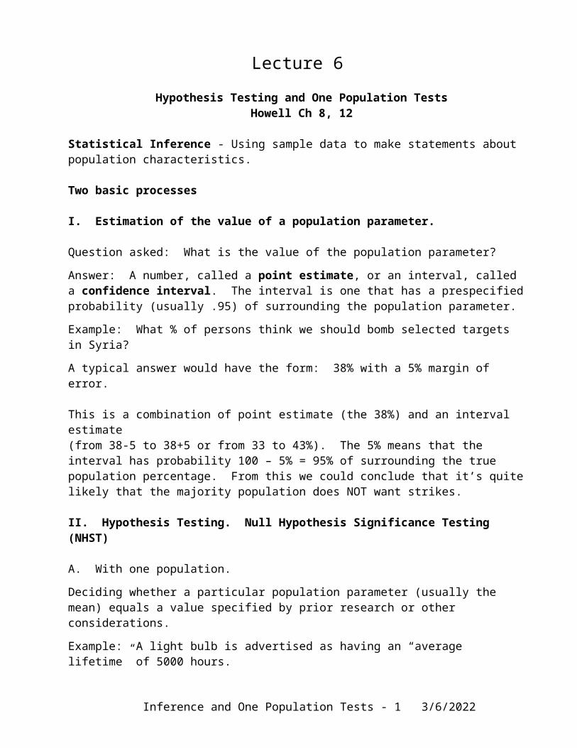
Determining when a tire is “worn out”.

Tire tread depth should be no less than 4/32”.

Place a quarter into several tread grooves across the tire. If part of Washington's head is always covered by the tread, you have more than 4/32" of tread depth remaining

Thanks to Dillon Brock, class of 2018.

Choosing the confidence interval level.

Hypothesis Testing and One Population Tests - 14 5/8/2023

Very Important. Put the hypothesized value of the population mean in the “Test Value” field.

Select the variable to be analyzed and move it to the “Test Variable(s)” field.

Click on the [Options] button to open the Confidence Interval dialog box.

The Output

T-TestOn e -Sa m p le Sta tis tic s

2 5 2 9 6 4 0 .0 0 8 9 9 .9 0 8 1 7 9 .9 8 2mi l e a g eN Me a n Std . De v i a t i o nStd . E rro r Me a n

O ne- Sam pl e Test

- 2. 000 24 . 057 - 360. 000 - 731. 46 11. 46m ileaget df Sig. ( 2- t ailed) M ean Dif f er ence Lower Upper

95% Conf idence I nt er val oft he Dif f er ence

Test Value = 30000

Actual Limits of Confidence Interval . . .

LL = -731.46 + 30,000 = 29,268.54

UL = 11.46 + 30,000 = 30,011.46


Value of t The two-tailed p-value.

Standardized Confidence interval.Add test value to each limit to get it in terms of the problem’s values.

Test value entered above.

Same Analysis using Rcmdr

R -> Rcmdr etc. etc. etc.Import Data -> from SPSS file . . .

Statistics -> Means -> Single-sample t-test

> mileage2 <- + read.spss("G:/MDBT/InClassDatasets/t test example 30000 miles tires .sav", + use.value.labels=TRUE, max.value.labels=Inf, to.data.frame=TRUE)

> colnames(mileage2) <- tolower(colnames(mileage2))

> with(mileage2, (t.test(mileage, alternative='two.sided', mu=30000, + conf.level=.95)))

One Sample t-test

data: mileaget = -2.0002, df = 24, p-value = 0.05692alternative hypothesis: true mean is not equal to 3000095 percent confidence interval: 29268.54 30011.46sample estimates:mean of x 29640


Hypotheses about the Population Correlation Coefficient, rAs I’ve mentioned a few times (and will mention many more times) one of the foundations of modern personality theory is the belief that there exist five basic personality traits – Extraversion, Agreebleness, Conscientiousness, Emotional Stability, and Openness to experience. Some believe there is a sixth – Honesty/Humility.

Most people would say that the Big Five personality traits do not include levels of affect. In fact, authors of some Big Five questionnaires have gone out of their way to exclude items which suggest affrect. The Big Five trait that some might think is measuring affective states is Emotional Stability. But most people regard Emotional Stability as measuring cognitive activity associated with problems in life, rather than levels of an affective state.

In our work with the Big Five and the HEXACO, we have computed a variable that we think represents the affective state of the respondent. This is computed from the responses participants made to the Big Five or HEXACO items, not responses to items added to the questionnaires.

In order to investigate what is called the nomlogical net of this variable, we correlated it with various measures of affect, specially, the Rosenberg Self-esteem Scale, the Comrey & Costello Depression scale, the PANAS PA scale and the PANAS NA scale.

If our new variable really measures affect, then it should correlate with each of these scales.

The results are below . . .


Affect variable from NEO Big Five Affect variable from HEXACO


Rosenberg

PA

Depression

r = .72

r = .68

r = -.70

r = .58

r = .54

r = -.63

Our new variable Our new variable


NA r = -.62 r = -.51



Testing Hypotheses on Population r

Step 1. Null Hypothesis: The population correlation coefficient is 0

Alternative Hypothesis: The population correlation coefficient is not 0.

Steps 2 and 3. Test statistics and sampling distribution: (There are two possibilities)

A) A t statistic

Sample r – 0 t = ---------------------- 1 – Sample r2

------------- N - 2

Critical t values would be obtained from tables of critical t.

B) r itself.

Step 4. The significance level would be .05, as is the convention.

Steps 5 and 6. We’ll use SPSS for these steps. p-values are in red.

SPSS AnalysesCorrelations – NEO variable

Mean of NEO RSE and HEX RSE scales.

Mean of NEO and HEX PA

scales.

Mean of ncc and hcc

scored so high scores mean

high depression.

Mean of NEO and HEX NA

scalesNEO mean M,Mp,Mn from ESEMTR O CR MMpMn n1195 data

Pearson Correlation .717 .682 -.701 -.622Sig. (2-tailed) .000 .000 .000 .000N 1195 1195 1195 1195

Correlations – HEXACO variable

Mean of NEO RSE and HEX RSE scales.

Mean of NEO and HEX PA

scales.

Mean of ncc and hcc

scored so high scores mean

high depression.

Mean of NEO and HEX NA

scalesHEX mean M,Mp,Mn from ESEMTR O CR MMpMn model

Pearson Correlation .578 .539 -.627 -.514Sig. (2-tailed) .000 .000 .000 .000N 1195 1195 1195 1195

Step 7. I reject the null hypothesis for each correlation.

Conclusion: The new affect variable we’ve computed from the Big Fiver and the HEXACO questionnaires seems to measure affect.


Documents

Probability - University of Tennessee at Chattanooga · Web viewExample: Statistics taught with lab vs. Statistics taught without lab. Question: Is the mean amount learned by the