Production Risers: A02 Midwater Arch Systems - Orcina · PDF fileProduction Risers: A02 Midwater Arch Systems Page 1 of 16 A02 Midwater Arch Systems Introduction In these examples,

W Orcina

Production Risers: A02 Midwater Arch Systems Page 1 of 16

A02 Midwater Arch Systems

Introduction

In these examples, three types of riser system are shown: a lazy S (both simple and detailed), a

steep S and a pliant S. An S configuration is similar to a catenary but has support provided at

about midwater by an arch structure.

On opening each simulation file, the default Workspace will present views in wireframe and

shaded graphics of the system.

The examples also show:

Modelling of midwater arches.

Contact between Lines and with Shapes, including friction.

Modelling bridles and tethers.

Using Supports to model arch gutters.

Setting the model north pointer.

W Orcina


1. Lazy S Simple

A lazy S configuration is similar to a catenary but has additional support provided at about

midwater by an arch structure. 'Lazy' means that the riser centreline is near parallel with the

seabed on contact while 'S' describes the line shape as a result of the arch.

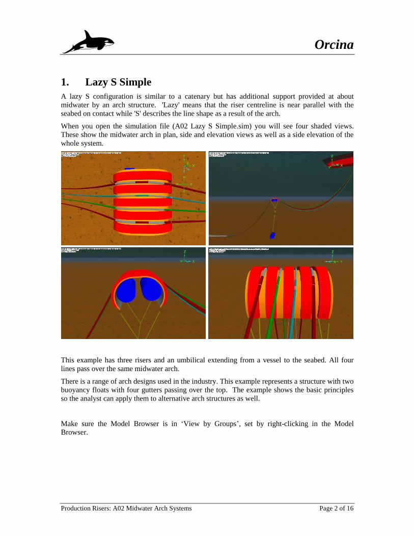
When you open the simulation file (A02 Lazy S Simple.sim) you will see four shaded views.

These show the midwater arch in plan, side and elevation views as well as a side elevation of the

whole system.

This example has three risers and an umbilical extending from a vessel to the seabed. All four

lines pass over the same midwater arch.

There is a range of arch designs used in the industry. This example represents a structure with two

buoyancy floats with four gutters passing over the top. The example shows the basic principles

so the analyst can apply them to alternative arch structures as well.

Make sure the Model Browser is in ‘View by Groups’, set by right-clicking in the Model

Browser.

W Orcina


1.1. Building the model

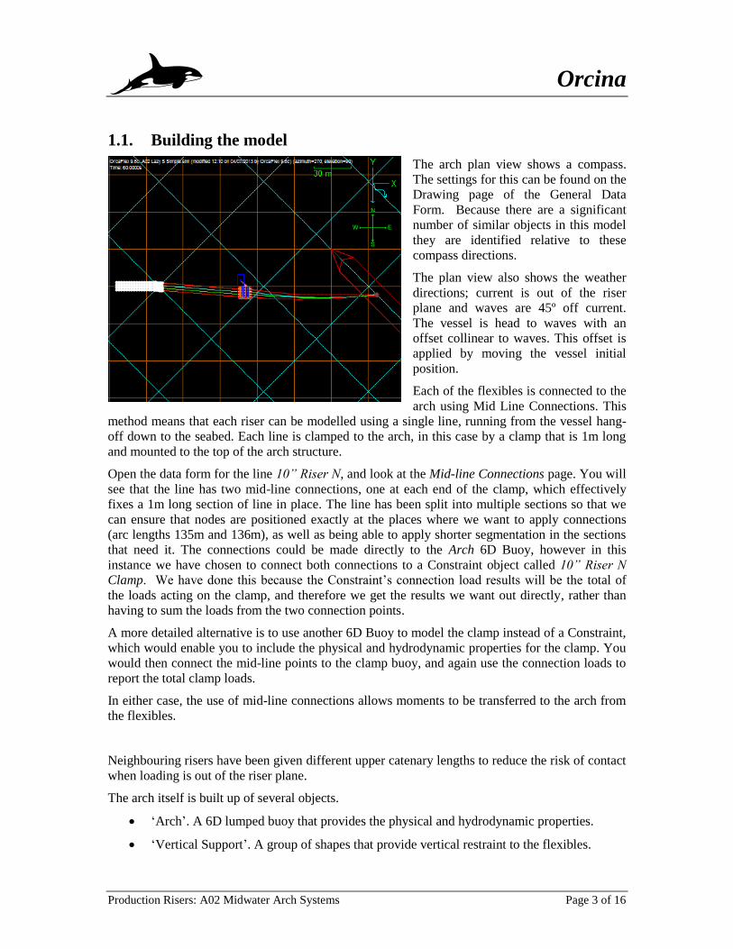
The arch plan view shows a compass.

The settings for this can be found on the

Drawing page of the General Data

Form. Because there are a significant

number of similar objects in this model

they are identified relative to these

compass directions.

The plan view also shows the weather

directions; current is out of the riser

plane and waves are 45º off current.

The vessel is head to waves with an

offset collinear to waves. This offset is

applied by moving the vessel initial

position.

Each of the flexibles is connected to the

arch using Mid Line Connections. This

method means that each riser can be modelled using a single line, running from the vessel hang-

off down to the seabed. Each line is clamped to the arch, in this case by a clamp that is 1m long

and mounted to the top of the arch structure.

Open the data form for the line 10” Riser N, and look at the Mid-line Connections page. You will

see that the line has two mid-line connections, one at each end of the clamp, which effectively

fixes a 1m long section of line in place. The line has been split into multiple sections so that we

can ensure that nodes are positioned exactly at the places where we want to apply connections

(arc lengths 135m and 136m), as well as being able to apply shorter segmentation in the sections

that need it. The connections could be made directly to the Arch 6D Buoy, however in this

instance we have chosen to connect both connections to a Constraint object called 10” Riser N

Clamp. We have done this because the Constraint’s connection load results will be the total of

the loads acting on the clamp, and therefore we get the results we want out directly, rather than

having to sum the loads from the two connection points.

A more detailed alternative is to use another 6D Buoy to model the clamp instead of a Constraint,

which would enable you to include the physical and hydrodynamic properties for the clamp. You

would then connect the mid-line points to the clamp buoy, and again use the connection loads to

report the total clamp loads.

In either case, the use of mid-line connections allows moments to be transferred to the arch from

the flexibles.

Neighbouring risers have been given different upper catenary lengths to reduce the risk of contact

when loading is out of the riser plane.

The arch itself is built up of several objects.

‘Arch’. A 6D lumped buoy that provides the physical and hydrodynamic properties.

‘Vertical Support’. A group of shapes that provide vertical restraint to the flexibles.

W Orcina


‘Horizontal Support’. A group of shapes that provide horizontal restraint to the flexibles.

‘Arch Drawings’. A group of shapes that provide the image of the arch structure.

‘Arch’ is a 6D (6 degrees of freedom) lumped buoy that contains the physical and hydrodynamic

properties of the whole arch structure. With this option, OrcaFlex requires you to determine these

overall properties.

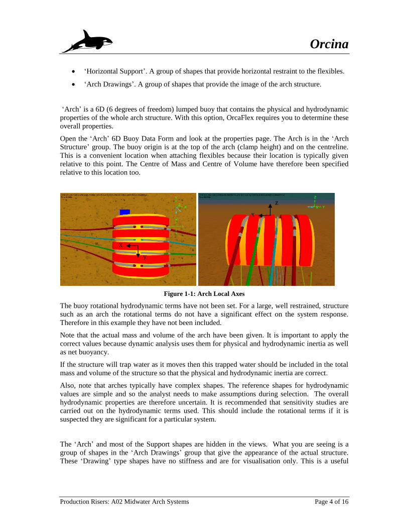
Open the ‘Arch’ 6D Buoy Data Form and look at the properties page. The Arch is in the ‘Arch

Structure’ group. The buoy origin is at the top of the arch (clamp height) and on the centreline.

This is a convenient location when attaching flexibles because their location is typically given

relative to this point. The Centre of Mass and Centre of Volume have therefore been specified

relative to this location too.

Figure 1-1: Arch Local Axes

The buoy rotational hydrodynamic terms have not been set. For a large, well restrained, structure

such as an arch the rotational terms do not have a significant effect on the system response.

Therefore in this example they have not been included.

Note that the actual mass and volume of the arch have been given. It is important to apply the

correct values because dynamic analysis uses them for physical and hydrodynamic inertia as well

as net buoyancy.

If the structure will trap water as it moves then this trapped water should be included in the total

mass and volume of the structure so that the physical and hydrodynamic inertia are correct.

Also, note that arches typically have complex shapes. The reference shapes for hydrodynamic

values are simple and so the analyst needs to make assumptions during selection. The overall

hydrodynamic properties are therefore uncertain. It is recommended that sensitivity studies are

carried out on the hydrodynamic terms used. This should include the rotational terms if it is

suspected they are significant for a particular system.

The ‘Arch’ and most of the Support shapes are hidden in the views. What you are seeing is a

group of shapes in the ‘Arch Drawings’ group that give the appearance of the actual structure.

These ‘Drawing’ type shapes have no stiffness and are for visualisation only. This is a useful

x

x

z

y

W Orcina


feature when presenting to clients who may not be analysts themselves. It allows them to see the

model in a way they are familiar with.

To see any hidden object right click on it in the Model Browser then select Show from the

dropdown menu. The same process but selecting Hide will make it invisible again. Note however

that Hide/Show only affects the views. The object is still present in the mathematical model and

will still affect the system.

The views below show the hidden support structure as it is built up.

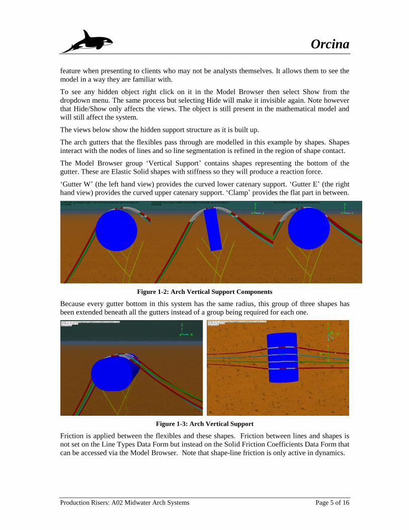
The arch gutters that the flexibles pass through are modelled in this example by shapes. Shapes

interact with the nodes of lines and so line segmentation is refined in the region of shape contact.

The Model Browser group ‘Vertical Support’ contains shapes representing the bottom of the

gutter. These are Elastic Solid shapes with stiffness so they will produce a reaction force.

‘Gutter W’ (the left hand view) provides the curved lower catenary support. ‘Gutter E’ (the right

hand view) provides the curved upper catenary support. ‘Clamp’ provides the flat part in between.

Figure 1-2: Arch Vertical Support Components

Because every gutter bottom in this system has the same radius, this group of three shapes has

been extended beneath all the gutters instead of a group being required for each one.

Figure 1-3: Arch Vertical Support

Friction is applied between the flexibles and these shapes. Friction between lines and shapes is

not set on the Line Types Data Form but instead on the Solid Friction Coefficients Data Form that

can be accessed via the Model Browser. Note that shape-line friction is only active in dynamics.

W Orcina


A very simple arch model might contain just these vertical supports. The risers are able to roll on

and off the arch, but the only lateral restraints while on the arch would be friction and the bend

stiffness of the riser. Riser curvature at the clamp location would therefore be highly

conservative.

Also all lateral moments would be transferred at the clamp connection only rather than distributed

along the gutter wall and so produce errors in the yaw response of the arch. Therefore it is

recommended that the gutter walls are represented in some form.

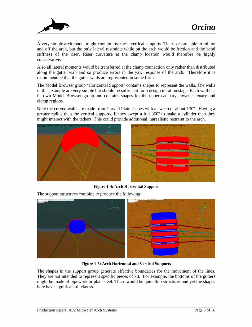
The Model Browser group ‘Horizontal Support’ contains shapes to represent the walls. The walls

in this example are very simple but should be sufficient for a design iteration stage. Each wall has

its own Model Browser group and contains shapes for the upper catenary, lower catenary and

clamp regions.

Note the curved walls are made from Curved Plate shapes with a sweep of about 130º. Having a

greater radius than the vertical supports, if they swept a full 360º to make a cylinder then they

might interact with the tethers. This could provide additional, unrealistic restraint to the arch.

Figure 1-4: Arch Horizontal Support

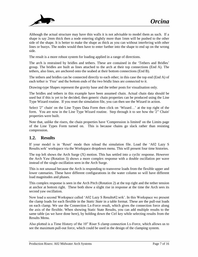
The support structures combine to produce the following:

Figure 1-5: Arch Horizontal and Vertical Supports

The shapes in the support group generate effective boundaries for the movement of the lines.

They are not intended to represent specific pieces of kit. For example, the bottoms of the gutters

might be made of pipework or plate steel. These would be quite thin structures and yet the shapes

here have significant thickness.

W Orcina


Although the actual structure may have thin walls it is not advisable to model them as such. If a

shape is say 2mm thick then a node entering slightly more than 1mm will be pushed to the other

side of the shape. It is better to make the shape as thick as you can without interfering with other

lines or buoys. The nodes would then have to enter further into the shape to end up on the wrong

side.

The result is a more robust system for loading applied in a range of directions.

The arch is restrained by bridles and tethers. These are contained in the ‘Tethers and Bridles’

group. The bridles are built as lines attached to the arch at their top connections (End A). The

tethers, also lines, are anchored onto the seabed at their bottom connections (End B).

The tethers and bridles can be connected directly to each other; in this case the top end (End A) of

each tether is ‘Free’ and the bottom ends of the two bridle lines are connected to it.

Drawing-type Shapes represent the gravity base and the tether posts for visualisation only.

The bridles and tethers in this example have been assumed chain. Actual chain data should be

used but if this is yet to be decided, then generic chain properties can be produced using the Line

Type Wizard routine. If you reset the simulation file, you can then see the Wizard in action.

Select '2” chain' on the Line Types Data Form then click on ‘Wizard…’ at the top right of the

form. You are now in the Line Type Wizard routine. Step through it to see how the '2” Chain'

properties were built.

Note that, unlike the risers, the chain properties have 'Compression is limited' on the Limits page

of the Line Types Form turned on. This is because chains go slack rather than resisting

compression.

1.2. Results

If your model is in ‘Reset’ mode then reload the simulation file. Load the ‘A02 Lazy S

Results.wrk’ workspace via the Workspace dropdown menu. This will present four time histories.

The top left shows the Arch Surge (X) motion. This has settled into a cyclic response. However

the Arch Yaw (Rotation 3) shows a more complex response with a double oscillation per wave

instead of the single oscillation seen in the Arch Surge.

This is not unusual because the Arch is responding to transverse loads from the flexible upper and

lower catenaries. These have different configurations in the water column so will have different

load magnitudes and phases.

This complex response is seen in the Arch Pitch (Rotation 2) at the top right and the tether tension

at anchor at bottom right. These both show a slight rise in response at the time the Arch sees its

second yaw oscillation.

Now load a second Workspace called ‘A02 Lazy S Results#2.wrk’. In this Workspace we present

the clamp loads for each flexible in the Static State in a table format. These are the pull-out loads

on each clamp. We use the Connection Lx-Force result, which gives the connection force along

the axis of the flexible. When showing Static State Results, you can add multiple results to the

same table (as we have done here), by holding down the Ctrl key while selecting results from the

Results Menu.

Also plotted is a Time History of the 10” Riser S clamp connection Lx-Force, which allows us to

see the maximum pull-out force, which could be used in the design of the clamping system.

W Orcina


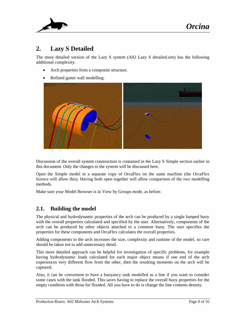
2. Lazy S Detailed

The more detailed version of the Lazy S system (A02 Lazy S detailed.sim) has the following

additional complexity.

Arch properties from a composite structure.

Refined gutter wall modelling.

Discussion of the overall system construction is contained in the Lazy S Simple section earlier in

this document. Only the changes to the system will be discussed here.

Open the Simple model in a separate copy of OrcaFlex on the same machine (the OrcaFlex

licence will allow this). Having both open together will allow comparison of the two modelling

methods.

Make sure your Model Browser is in View by Groups mode, as before.


The physical and hydrodynamic properties of the arch can be produced by a single lumped buoy

with the overall properties calculated and specified by the user. Alternatively, components of the

arch can be produced by other objects attached to a common buoy. The user specifies the

properties for these components and OrcaFlex calculates the overall properties.

Adding components to the arch increases the size, complexity and runtime of the model, so care

should be taken not to add unnecessary detail.

This more detailed approach can be helpful for investigation of specific problems, for example

having hydrodynamic loads calculated for each major object means if one end of the arch

experiences very different flow from the other, then the resulting moments on the arch will be

captured.

Also, it can be convenient to have a buoyancy tank modelled as a line if you want to consider

some cases with the tank flooded. This saves having to replace the overall buoy properties for the

empty condition with those for flooded. All you have to do is change the line contents density.

W Orcina


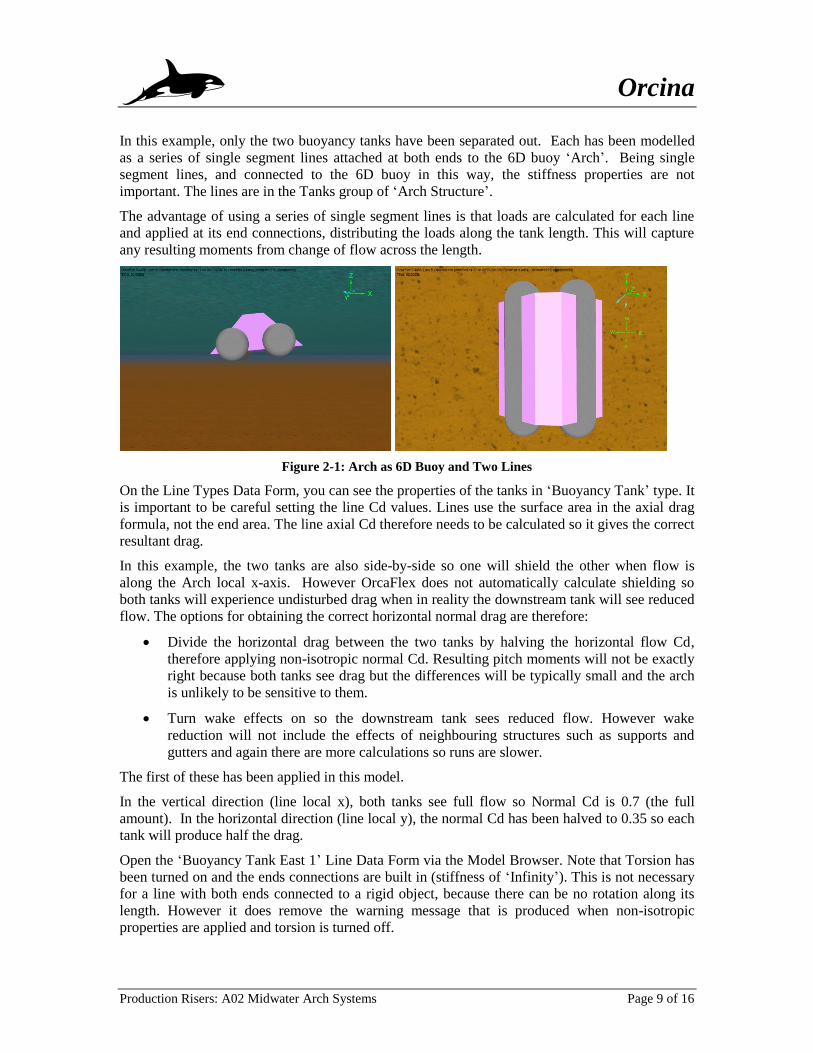
In this example, only the two buoyancy tanks have been separated out. Each has been modelled

as a series of single segment lines attached at both ends to the 6D buoy ‘Arch’. Being single

segment lines, and connected to the 6D buoy in this way, the stiffness properties are not

important. The lines are in the Tanks group of ‘Arch Structure’.

The advantage of using a series of single segment lines is that loads are calculated for each line

and applied at its end connections, distributing the loads along the tank length. This will capture

any resulting moments from change of flow across the length.

Figure 2-1: Arch as 6D Buoy and Two Lines

On the Line Types Data Form, you can see the properties of the tanks in ‘Buoyancy Tank’ type. It

is important to be careful setting the line Cd values. Lines use the surface area in the axial drag

formula, not the end area. The line axial Cd therefore needs to be calculated so it gives the correct

resultant drag.

In this example, the two tanks are also side-by-side so one will shield the other when flow is

along the Arch local x-axis. However OrcaFlex does not automatically calculate shielding so

both tanks will experience undisturbed drag when in reality the downstream tank will see reduced

flow. The options for obtaining the correct horizontal normal drag are therefore:

Divide the horizontal drag between the two tanks by halving the horizontal flow Cd,

therefore applying non-isotropic normal Cd. Resulting pitch moments will not be exactly

right because both tanks see drag but the differences will be typically small and the arch

is unlikely to be sensitive to them.

Turn wake effects on so the downstream tank sees reduced flow. However wake

reduction will not include the effects of neighbouring structures such as supports and

gutters and again there are more calculations so runs are slower.

The first of these has been applied in this model.

In the vertical direction (line local x), both tanks see full flow so Normal Cd is 0.7 (the full

amount). In the horizontal direction (line local y), the normal Cd has been halved to 0.35 so each

tank will produce half the drag.

Open the ‘Buoyancy Tank East 1’ Line Data Form via the Model Browser. Note that Torsion has

been turned on and the ends connections are built in (stiffness of ‘Infinity’). This is not necessary

for a line with both ends connected to a rigid object, because there can be no rotation along its

length. However it does remove the warning message that is produced when non-isotropic

properties are applied and torsion is turned off.

W Orcina


The remainder of the arch properties are then calculated and applied to the 6D buoy so the

resultant physical and hydrodynamic properties match those used in the simple model.

Compare the data for the Arch buoy in the two models. Taking away the tank contributions has

changed the volume, mass, moments of inertia, centre of mass and volume and the drag areas. In

this simplistic example, the mass has reduced by approximately a factor of ten, therefore we have

reduced the mass moments of inertia by the same factor.

Note the line objects have been hidden from view and Drawing shapes have been used for

visualisation in this example. For more information on hiding and showing objects, see the Lazy

S Simple model discussion earlier in this document.

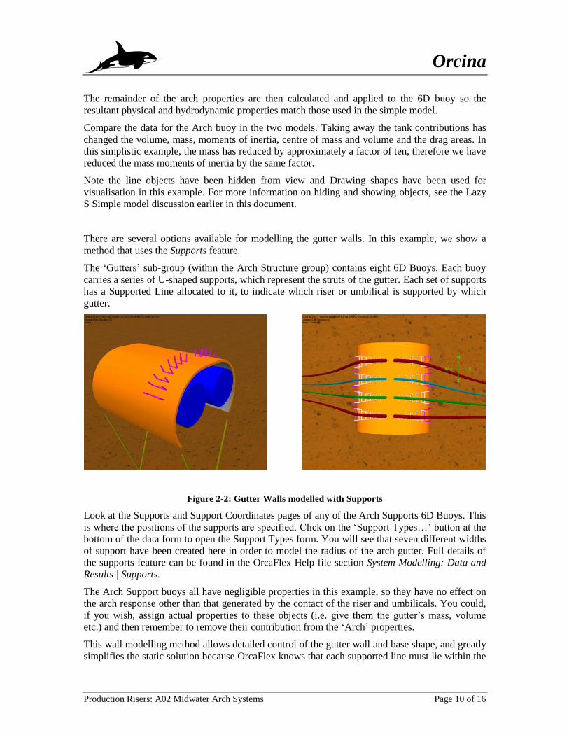
There are several options available for modelling the gutter walls. In this example, we show a

method that uses the Supports feature.

The ‘Gutters’ sub-group (within the Arch Structure group) contains eight 6D Buoys. Each buoy

carries a series of U-shaped supports, which represent the struts of the gutter. Each set of supports

has a Supported Line allocated to it, to indicate which riser or umbilical is supported by which

gutter.

Figure 2-2: Gutter Walls modelled with Supports

Look at the Supports and Support Coordinates pages of any of the Arch Supports 6D Buoys. This

is where the positions of the supports are specified. Click on the ‘Support Types…’ button at the

bottom of the data form to open the Support Types form. You will see that seven different widths

of support have been created here in order to model the radius of the arch gutter. Full details of

the supports feature can be found in the OrcaFlex Help file section System Modelling: Data and

Results | Supports.

The Arch Support buoys all have negligible properties in this example, so they have no effect on

the arch response other than that generated by the contact of the riser and umbilicals. You could,

if you wish, assign actual properties to these objects (i.e. give them the gutter’s mass, volume

etc.) and then remember to remove their contribution from the ‘Arch’ properties.

This wall modelling method allows detailed control of the gutter wall and base shape, and greatly

simplifies the static solution because OrcaFlex knows that each supported line must lie within the

W Orcina


set of supports to which it is assigned. To demonstrate this, reset the model (press F12) and then

re-run the static calculation by pressing F9. You will see the eight riser and umbilical lines jump

very quickly into place within the gutter boundaries.

Available results for the supports include clearance and lift out results, as well as reaction force

results for individual supports or for entire sets of supports. Open the workspace file ‘A02 Lazy S

Supports.wrk’ to see the support force and lift out results for the lower 10” N riser.

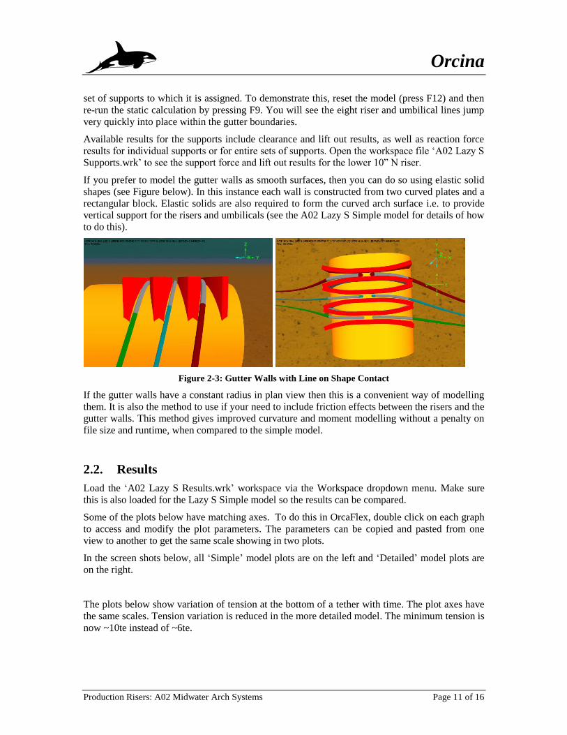
If you prefer to model the gutter walls as smooth surfaces, then you can do so using elastic solid

shapes (see Figure below). In this instance each wall is constructed from two curved plates and a

rectangular block. Elastic solids are also required to form the curved arch surface i.e. to provide

vertical support for the risers and umbilicals (see the A02 Lazy S Simple model for details of how

to do this).

Figure 2-3: Gutter Walls with Line on Shape Contact

If the gutter walls have a constant radius in plan view then this is a convenient way of modelling

them. It is also the method to use if your need to include friction effects between the risers and the

gutter walls. This method gives improved curvature and moment modelling without a penalty on

file size and runtime, when compared to the simple model.

2.2. Results

Load the ‘A02 Lazy S Results.wrk’ workspace via the Workspace dropdown menu. Make sure

this is also loaded for the Lazy S Simple model so the results can be compared.

Some of the plots below have matching axes. To do this in OrcaFlex, double click on each graph

to access and modify the plot parameters. The parameters can be copied and pasted from one

view to another to get the same scale showing in two plots.

In the screen shots below, all ‘Simple’ model plots are on the left and ‘Detailed’ model plots are

on the right.

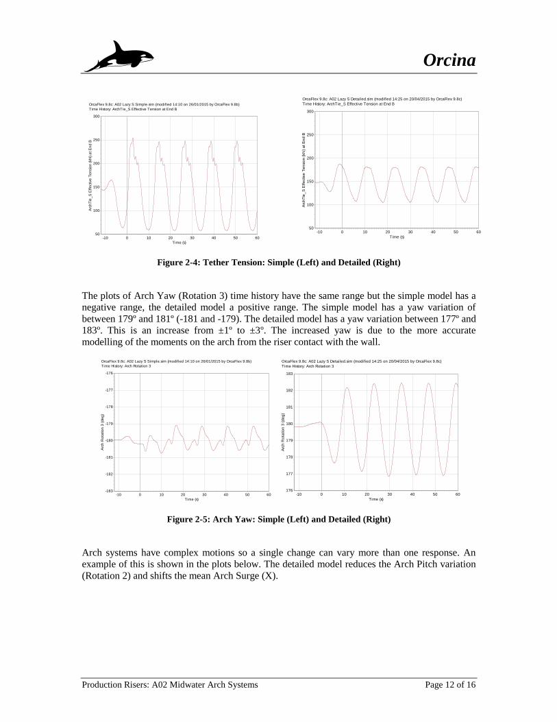
The plots below show variation of tension at the bottom of a tether with time. The plot axes have

the same scales. Tension variation is reduced in the more detailed model. The minimum tension is

now ~10te instead of ~6te.

W Orcina


OrcaFlex 9.8c: A02 Lazy S Simple.sim (modified 14:10 on 26/01/2015 by OrcaFlex 9.8b)

Time History: ArchTie_S Effective Tension at End B

Time (s)

6050403020100-10

Arc

hT

ie_

S E

ffe

ctive

Te

nsio

n (

kN

) a

t E

nd

B

300

250

200

150

100

50

OrcaFlex 9.8c: A02 Lazy S Detailed.sim (modified 14:25 on 20/04/2015 by OrcaFlex 9.8c)

Time History: ArchTie_S Effective Tension at End B

Time (s)

6050403020100-10

Arc

hT

ie_

S E

ffe

ctive

Te

nsio

n (

kN

) a

t E

nd

B

300

250

200

150

100

50

Figure 2-4: Tether Tension: Simple (Left) and Detailed (Right)

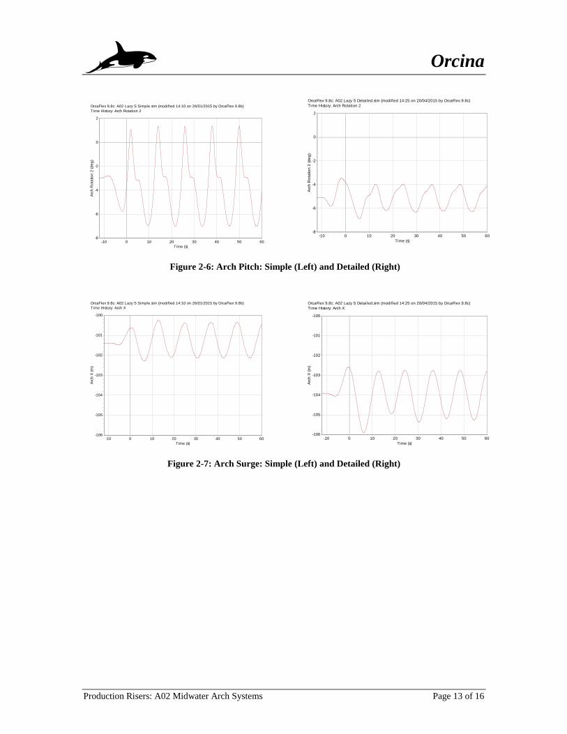
The plots of Arch Yaw (Rotation 3) time history have the same range but the simple model has a

negative range, the detailed model a positive range. The simple model has a yaw variation of

between 179º and 181º (-181 and -179). The detailed model has a yaw variation between 177º and

183º. This is an increase from ±1º to ±3º. The increased yaw is due to the more accurate

modelling of the moments on the arch from the riser contact with the wall.


Time History: Arch Rotation 3

Time (s)

6050403020100-10

Arc

h R

ota

tio

n 3

(d

eg

)

-176

-177

-178

-179

-180

-181

-182

-183



Time (s)

6050403020100-10

Arc

h R

ota

tio

n 3

(d

eg

)

183

182

181

180

179

178

177

176

Figure 2-5: Arch Yaw: Simple (Left) and Detailed (Right)

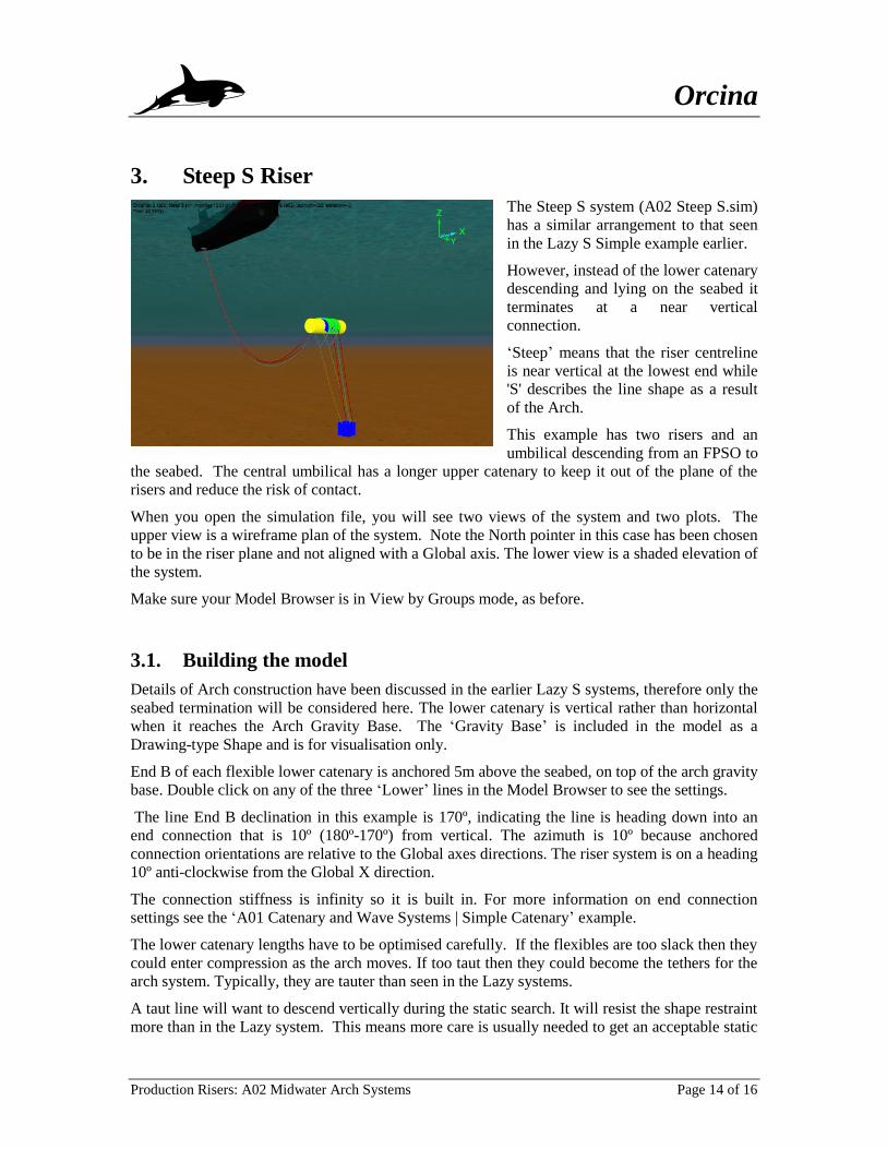
Arch systems have complex motions so a single change can vary more than one response. An

example of this is shown in the plots below. The detailed model reduces the Arch Pitch variation

(Rotation 2) and shifts the mean Arch Surge (X).

W Orcina




Time (s)

6050403020100-10

Arc

h R

ota

tio

n 2

(d

eg

)

2

0

-2

-4

-6

-8



Time (s)

6050403020100-10

Arc

h R

ota

tio

n 2

(d

eg

)

2

0

-2

-4

-6

-8

Figure 2-6: Arch Pitch: Simple (Left) and Detailed (Right)


Time History: Arch X

Time (s)

6050403020100-10

Arc

h X

(m

)

-100

-101

-102

-103

-104

-105

-106


Time History: Arch X

Time (s)

6050403020100-10

Arc

h X

(m

)

-100

-101

-102

-103

-104

-105

-106

Figure 2-7: Arch Surge: Simple (Left) and Detailed (Right)

W Orcina


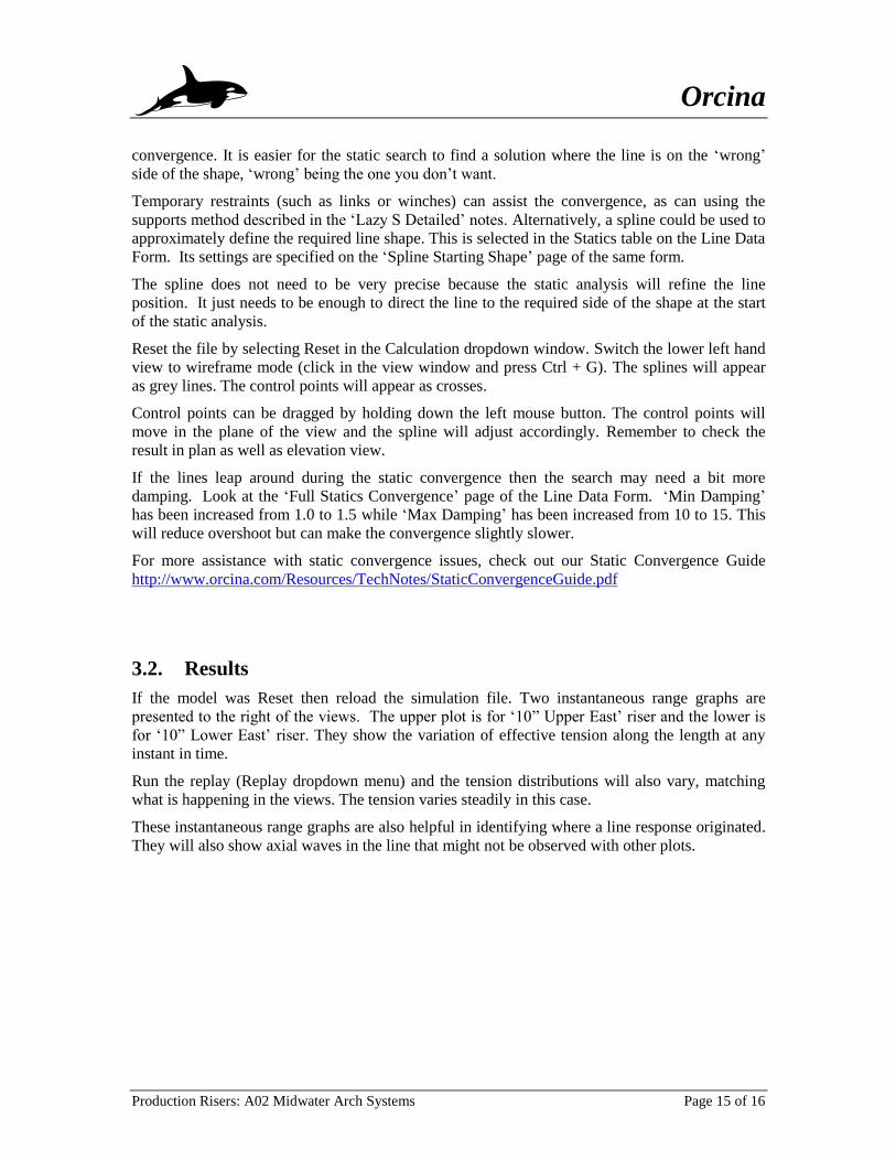
3. Steep S Riser

The Steep S system (A02 Steep S.sim)

has a similar arrangement to that seen

in the Lazy S Simple example earlier.

However, instead of the lower catenary

descending and lying on the seabed it

terminates at a near vertical

connection.

‘Steep’ means that the riser centreline

is near vertical at the lowest end while

'S' describes the line shape as a result

of the Arch.

This example has two risers and an

umbilical descending from an FPSO to

the seabed. The central umbilical has a longer upper catenary to keep it out of the plane of the

risers and reduce the risk of contact.

When you open the simulation file, you will see two views of the system and two plots. The

upper view is a wireframe plan of the system. Note the North pointer in this case has been chosen

to be in the riser plane and not aligned with a Global axis. The lower view is a shaded elevation of

the system.



Details of Arch construction have been discussed in the earlier Lazy S systems, therefore only the

seabed termination will be considered here. The lower catenary is vertical rather than horizontal

when it reaches the Arch Gravity Base. The ‘Gravity Base’ is included in the model as a

Drawing-type Shape and is for visualisation only.

End B of each flexible lower catenary is anchored 5m above the seabed, on top of the arch gravity

base. Double click on any of the three ‘Lower’ lines in the Model Browser to see the settings.

The line End B declination in this example is 170º, indicating the line is heading down into an

end connection that is 10º (180º-170º) from vertical. The azimuth is 10º because anchored

connection orientations are relative to the Global axes directions. The riser system is on a heading

10º anti-clockwise from the Global X direction.

The connection stiffness is infinity so it is built in. For more information on end connection

settings see the ‘A01 Catenary and Wave Systems | Simple Catenary’ example.

The lower catenary lengths have to be optimised carefully. If the flexibles are too slack then they

could enter compression as the arch moves. If too taut then they could become the tethers for the

arch system. Typically, they are tauter than seen in the Lazy systems.

A taut line will want to descend vertically during the static search. It will resist the shape restraint

more than in the Lazy system. This means more care is usually needed to get an acceptable static

W Orcina


convergence. It is easier for the static search to find a solution where the line is on the ‘wrong’

side of the shape, ‘wrong’ being the one you don’t want.

Temporary restraints (such as links or winches) can assist the convergence, as can using the

supports method described in the ‘Lazy S Detailed’ notes. Alternatively, a spline could be used to

approximately define the required line shape. This is selected in the Statics table on the Line Data

Form. Its settings are specified on the ‘Spline Starting Shape’ page of the same form.

The spline does not need to be very precise because the static analysis will refine the line

position. It just needs to be enough to direct the line to the required side of the shape at the start

of the static analysis.

Reset the file by selecting Reset in the Calculation dropdown window. Switch the lower left hand

view to wireframe mode (click in the view window and press Ctrl + G). The splines will appear

as grey lines. The control points will appear as crosses.

Control points can be dragged by holding down the left mouse button. The control points will

move in the plane of the view and the spline will adjust accordingly. Remember to check the

result in plan as well as elevation view.

If the lines leap around during the static convergence then the search may need a bit more

damping. Look at the ‘Full Statics Convergence’ page of the Line Data Form. ‘Min Damping’

has been increased from 1.0 to 1.5 while ‘Max Damping’ has been increased from 10 to 15. This

will reduce overshoot but can make the convergence slightly slower.

For more assistance with static convergence issues, check out our Static Convergence Guide

http://www.orcina.com/Resources/TechNotes/StaticConvergenceGuide.pdf

3.2. Results

If the model was Reset then reload the simulation file. Two instantaneous range graphs are

presented to the right of the views. The upper plot is for ‘10” Upper East’ riser and the lower is

for ‘10” Lower East’ riser. They show the variation of effective tension along the length at any

instant in time.

Run the replay (Replay dropdown menu) and the tension distributions will also vary, matching

what is happening in the views. The tension varies steadily in this case.

These instantaneous range graphs are also helpful in identifying where a line response originated.

They will also show axial waves in the line that might not be observed with other plots.

http://www.orcina.com/Resources/TechNotes/StaticConvergenceGuide.pdf

W Orcina


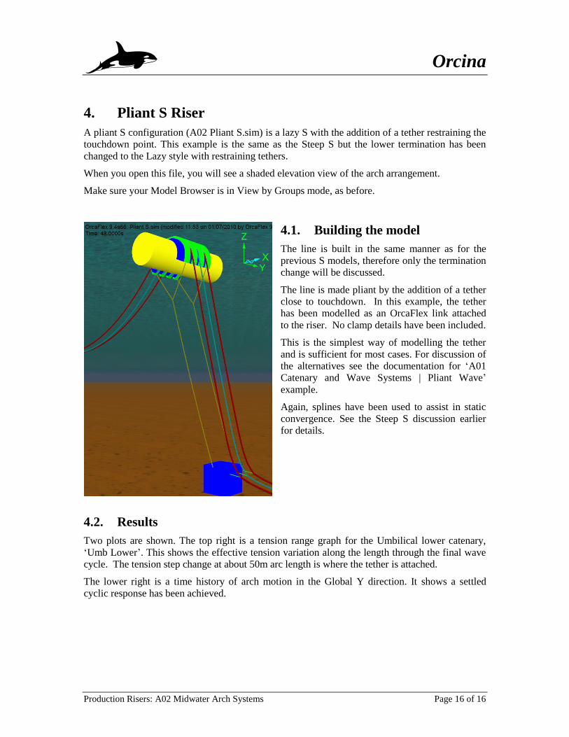
4. Pliant S Riser

A pliant S configuration (A02 Pliant S.sim) is a lazy S with the addition of a tether restraining the

touchdown point. This example is the same as the Steep S but the lower termination has been

changed to the Lazy style with restraining tethers.

When you open this file, you will see a shaded elevation view of the arch arrangement.



The line is built in the same manner as for the

previous S models, therefore only the termination

change will be discussed.

The line is made pliant by the addition of a tether

close to touchdown. In this example, the tether

has been modelled as an OrcaFlex link attached

to the riser. No clamp details have been included.

This is the simplest way of modelling the tether

and is sufficient for most cases. For discussion of

the alternatives see the documentation for ‘A01

Catenary and Wave Systems | Pliant Wave’

example.

Again, splines have been used to assist in static

convergence. See the Steep S discussion earlier

for details.

4.2. Results

Two plots are shown. The top right is a tension range graph for the Umbilical lower catenary,

‘Umb Lower’. This shows the effective tension variation along the length through the final wave

cycle. The tension step change at about 50m arc length is where the tether is attached.

The lower right is a time history of arch motion in the Global Y direction. It shows a settled

cyclic response has been achieved.

Documents

Production Risers: A02 Midwater Arch Systems - Orcina · PDF fileProduction Risers: A02 Midwater Arch Systems Page 1 of 16 A02 Midwater Arch Systems Introduction In these examples,