Prof. Bodik CS 164 Lecture 16, Fall 20041 Intermediate Code. Local Optimizations Lecture 15

Prof. Bodik CS 164 Lecture 16, Fall 2004 1

Intermediate Code. Local Optimizations

Lecture 15

Prof. Bodik CS 164 Lecture 16, Fall 2004

2

Lecture Outline

• Intermediate code

• Local optimizations

• Next time: global optimizations


3

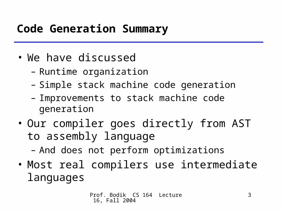
Code Generation Summary

• We have discussed– Runtime organization– Simple stack machine code generation– Improvements to stack machine code

generation

• Our compiler goes directly from AST to assembly language– And does not perform optimizations

• Most real compilers use intermediate languages


4

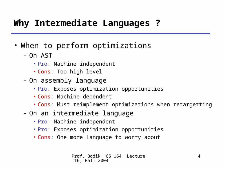
Why Intermediate Languages ?

• When to perform optimizations– On AST

• Pro: Machine independent• Cons: Too high level

– On assembly language• Pro: Exposes optimization opportunities• Cons: Machine dependent• Cons: Must reimplement optimizations when retargetting

– On an intermediate language• Pro: Machine independent• Pro: Exposes optimization opportunities• Cons: One more language to worry about


5

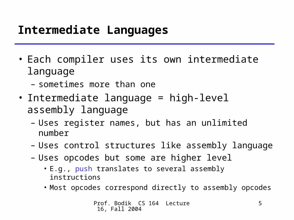
Intermediate Languages

• Each compiler uses its own intermediate language– sometimes more than one

• Intermediate language = high-level assembly language– Uses register names, but has an unlimited

number– Uses control structures like assembly language– Uses opcodes but some are higher level

• E.g., push translates to several assembly instructions• Most opcodes correspond directly to assembly opcodes


6

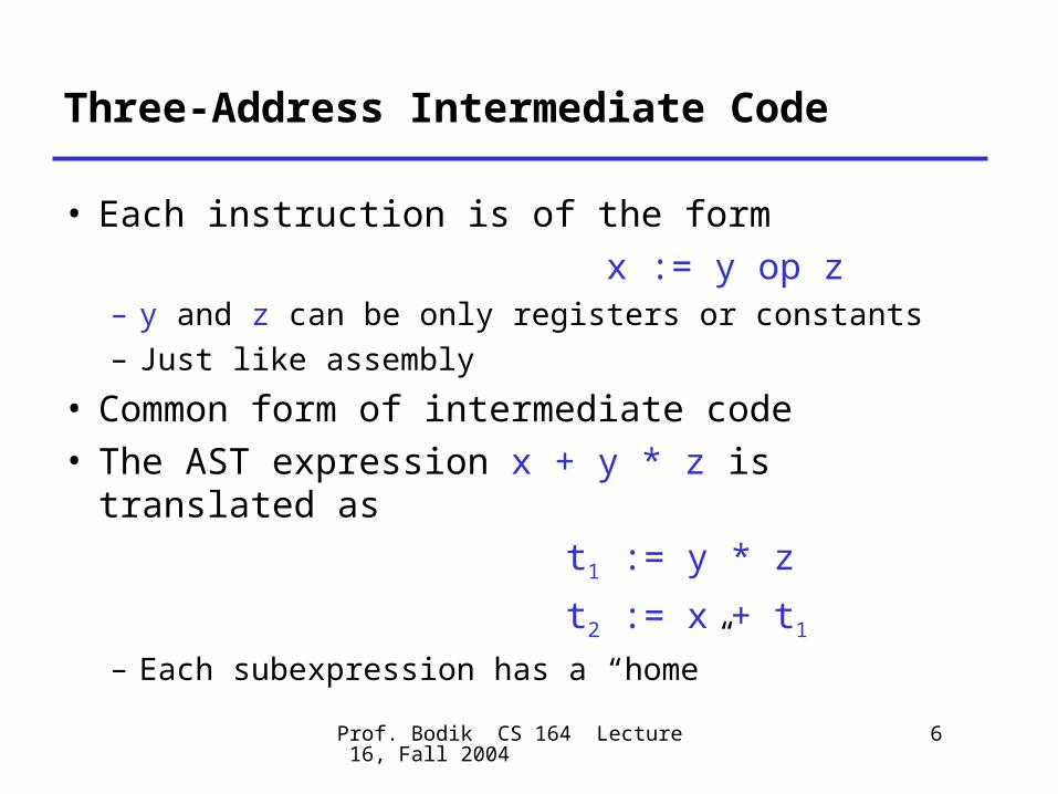
Three-Address Intermediate Code

• Each instruction is of the form x := y op z

– y and z can be only registers or constants– Just like assembly

• Common form of intermediate code• The AST expression x + y * z is translated as

t1 := y * z

t2 := x + t1

– Each subexpression has a “home”


7

Generating Intermediate Code

• Similar to assembly code generation• Major difference

– Use any number of IL registers to hold intermediate results


8

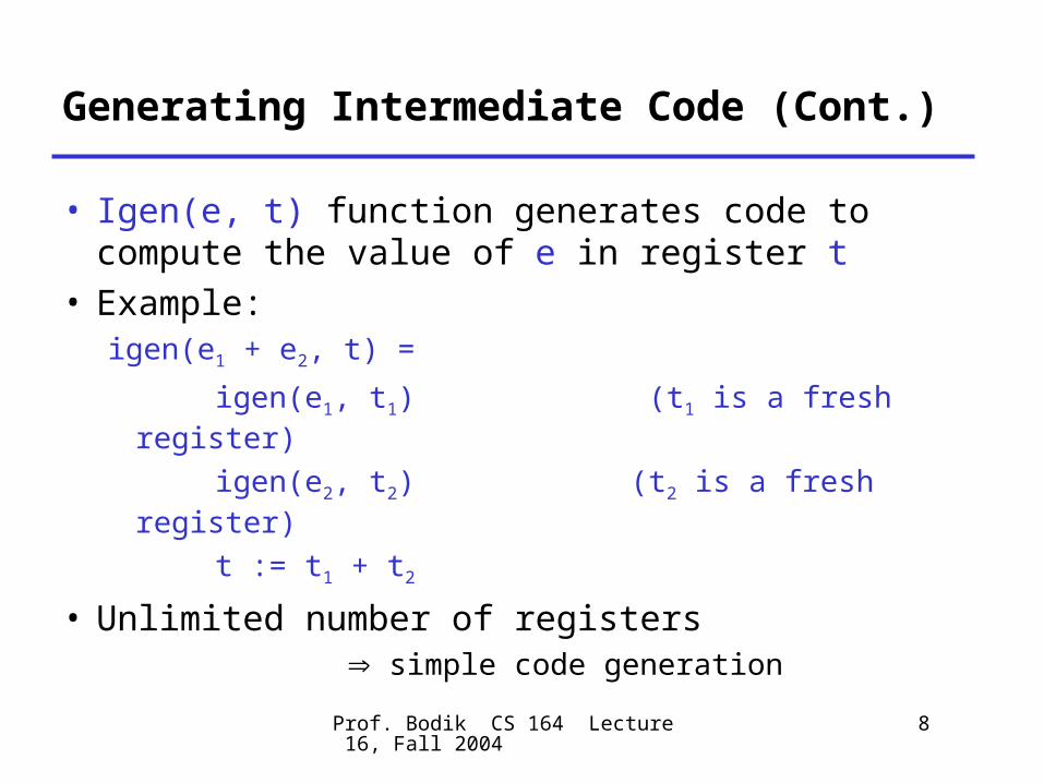
Generating Intermediate Code (Cont.)

• Igen(e, t) function generates code to compute the value of e in register t

• Example:igen(e1 + e2, t) =

igen(e1, t1) (t1 is a fresh register)

igen(e2, t2) (t2 is a fresh register)

t := t1 + t2

• Unlimited number of registers simple code generation


9

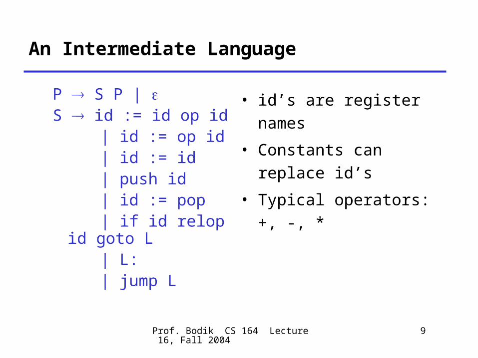
An Intermediate Language

P S P | S id := id op id | id := op id | id := id | push id | id := pop | if id relop id goto

L | L: | jump L

• id’s are register names

• Constants can replace id’s

• Typical operators: +, -, *


10

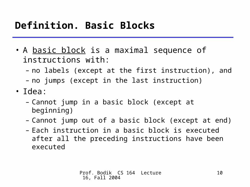
Definition. Basic Blocks

• A basic block is a maximal sequence of instructions with: – no labels (except at the first instruction), and – no jumps (except in the last instruction)

• Idea: – Cannot jump in a basic block (except at beginning)– Cannot jump out of a basic block (except at end)– Each instruction in a basic block is executed after all

the preceding instructions have been executed


11

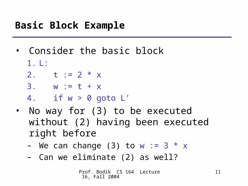
Basic Block Example

• Consider the basic block1. L: 2. t := 2 * x3. w := t + x4. if w > 0 goto L’

• No way for (3) to be executed without (2) having been executed right before– We can change (3) to w := 3 * x– Can we eliminate (2) as well?


12

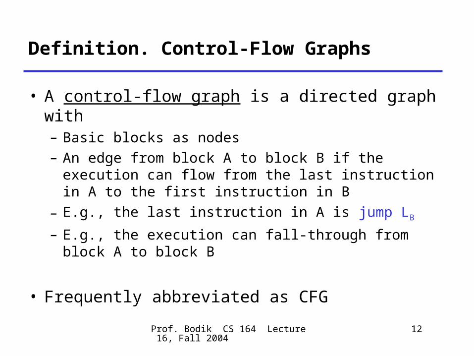
Definition. Control-Flow Graphs

• A control-flow graph is a directed graph with– Basic blocks as nodes– An edge from block A to block B if the execution

can flow from the last instruction in A to the first instruction in B

– E.g., the last instruction in A is jump LB

– E.g., the execution can fall-through from block A to block B

• Frequently abbreviated as CFG


13

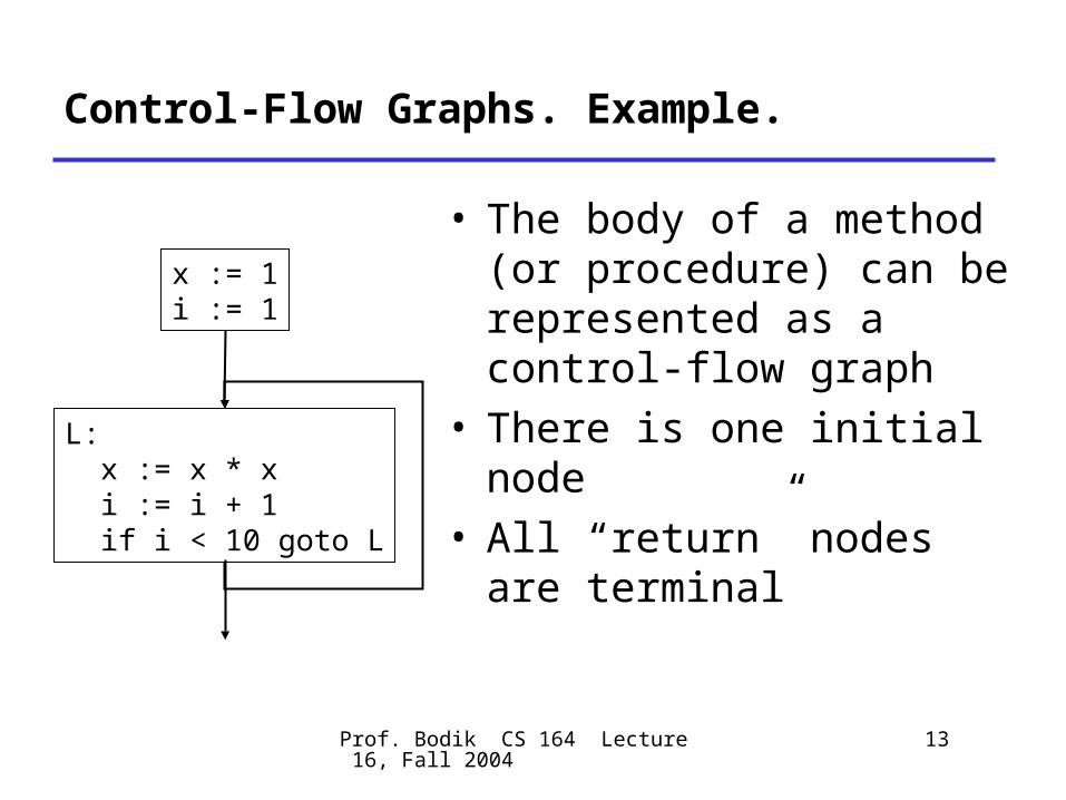
Control-Flow Graphs. Example.

• The body of a method (or procedure) can be represented as a control-flow graph

• There is one initial node• All “return” nodes are

terminal

x := 1i := 1

L: x := x * x i := i + 1 if i < 10 goto L


14

Optimization Overview

• Optimization seeks to improve a program’s utilization of some resource– Execution time (most often)– Code size– Network messages sent– Battery power used, etc.

• Optimization should not alter what the program computes– The answer must still be the same


15

A Classification of Optimizations

• For languages like C and Decaf there are three granularities of optimizations1. Local optimizations

• Apply to a basic block in isolation

2. Global optimizations• Apply to a control-flow graph (method body) in

isolation

3. Inter-procedural optimizations• Apply across method boundaries

• Most compilers do (1), many do (2) and a few do (3)


16

Cost of Optimizations

• In practice, a conscious decision is made not to implement the fanciest optimization known

• Why?– Some optimizations are hard to implement– Some optimizations are costly in terms of

compilation time– The fancy optimizations are both hard and costly

• The goal: maximum improvement with minimum of cost


17

Local Optimizations

• The simplest form of optimizations• No need to analyze the whole procedure

body– Just the basic block in question

• Example: algebraic simplification


18

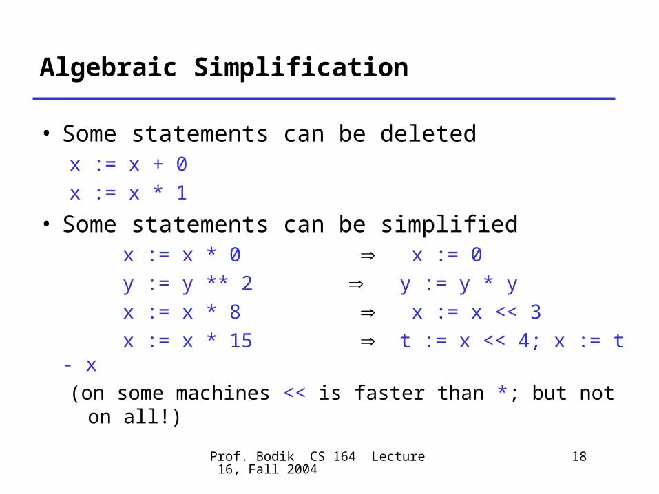
Algebraic Simplification

• Some statements can be deletedx := x + 0x := x * 1

• Some statements can be simplified x := x * 0 x := 0 y := y ** 2 y := y * y x := x * 8 x := x << 3 x := x * 15 t := x << 4; x := t - x

(on some machines << is faster than *; but not on all!)


19

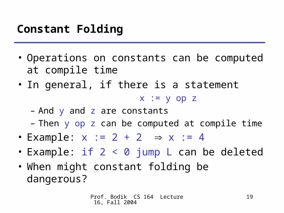
Constant Folding

• Operations on constants can be computed at compile time

• In general, if there is a statement x := y op z– And y and z are constants– Then y op z can be computed at compile time

• Example: x := 2 + 2 x := 4• Example: if 2 < 0 jump L can be deleted• When might constant folding be dangerous?


20

Flow of Control Optimizations

• Eliminating unreachable code:– Code that is unreachable in the control-flow graph– Basic blocks that are not the target of any jump

or “fall through” from a conditional– Such basic blocks can be eliminated

• Why would such basic blocks occur?• Removing unreachable code makes the

program smaller– And sometimes also faster

• Due to memory cache effects (increased spatial locality)


21

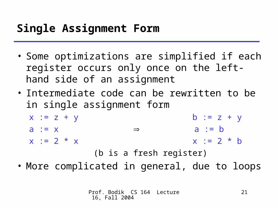
Single Assignment Form

• Some optimizations are simplified if each register occurs only once on the left-hand side of an assignment

• Intermediate code can be rewritten to be in single assignment formx := z + y b := z + ya := x a := bx := 2 * x x := 2 * b (b is a fresh register)

• More complicated in general, due to loops


22

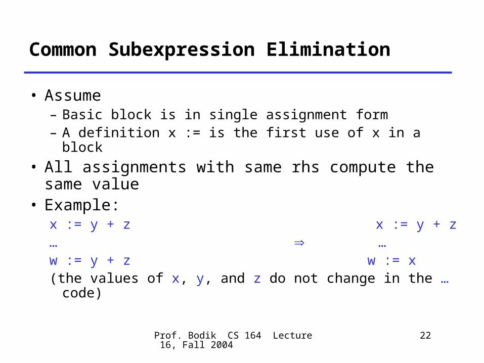
Common Subexpression Elimination

• Assume– Basic block is in single assignment form– A definition x := is the first use of x in a block

• All assignments with same rhs compute the same value

• Example:x := y + z x := y + z… …w := y + z w := x(the values of x, y, and z do not change in the …

code)


23

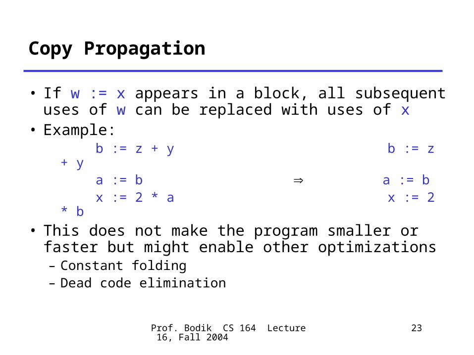
Copy Propagation

• If w := x appears in a block, all subsequent uses of w can be replaced with uses of x

• Example: b := z + y b := z + y a := b a := b x := 2 * a x := 2 * b

• This does not make the program smaller or faster but might enable other optimizations– Constant folding– Dead code elimination


24

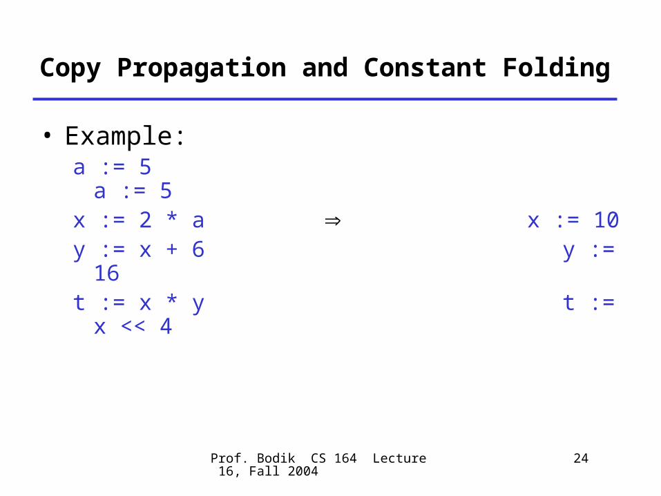
Copy Propagation and Constant Folding

• Example:a := 5 a := 5x := 2 * a x := 10y := x + 6 y := 16t := x * y t := x << 4


25

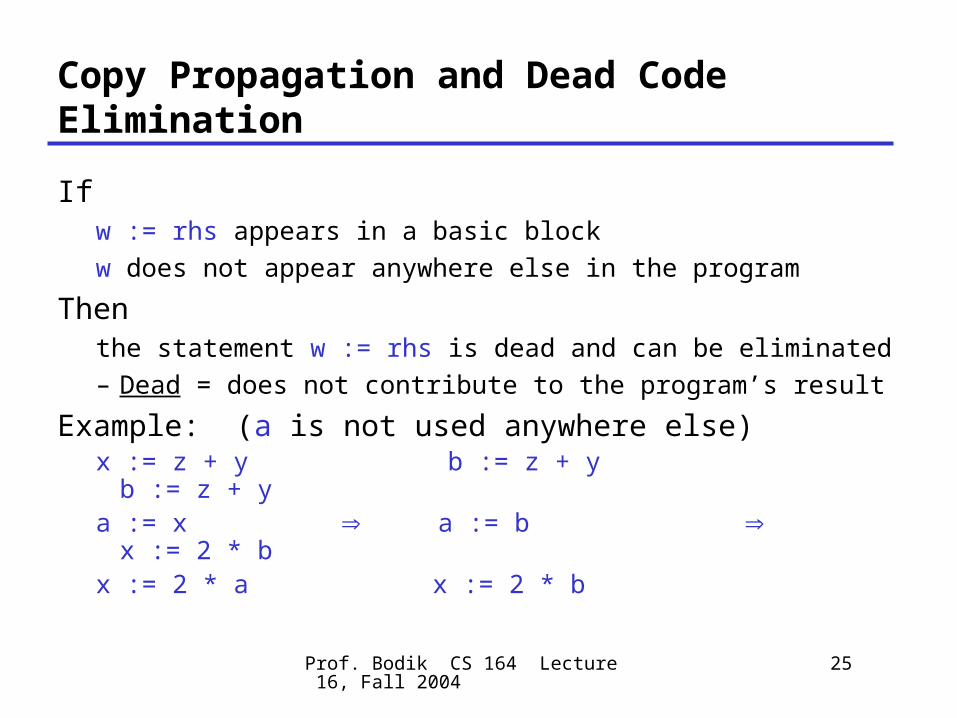
Copy Propagation and Dead Code Elimination

If w := rhs appears in a basic blockw does not appear anywhere else in the program

Then the statement w := rhs is dead and can be

eliminated– Dead = does not contribute to the program’s result

Example: (a is not used anywhere else)x := z + y b := z + y b := z + ya := x a := b x := 2 * bx := 2 * a x := 2 * b


26

Applying Local Optimizations

• Each local optimization does very little by itself

• Typically optimizations interact– Performing one optimizations enables other

opt.

• Typical optimizing compilers repeatedly perform optimizations until no improvement is possible– The optimizer can also be stopped at any time

to limit the compilation time


27

An Example

• Initial code: a := x ** 2 b := 3 c := x d := c * c e := b * 2 f := a + d g := e * f


28

An Example

• Algebraic optimization: a := x ** 2 b := 3 c := x d := c * c e := b * 2 f := a + d g := e * f


29

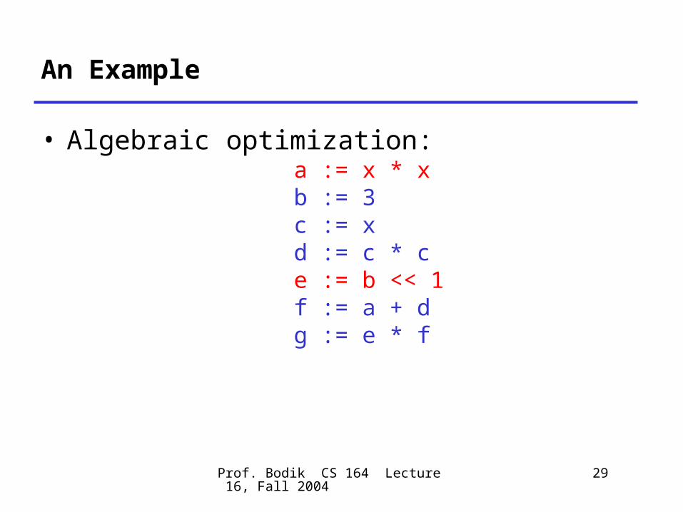
An Example

• Algebraic optimization: a := x * x b := 3 c := x d := c * c e := b << 1 f := a + d g := e * f


30

An Example

• Copy propagation: a := x * x b := 3 c := x d := c * c e := b << 1 f := a + d g := e * f


31

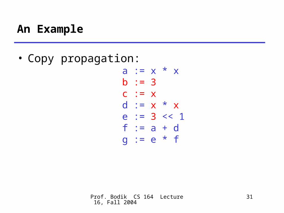
An Example

• Copy propagation: a := x * x b := 3 c := x d := x * x e := 3 << 1 f := a + d g := e * f


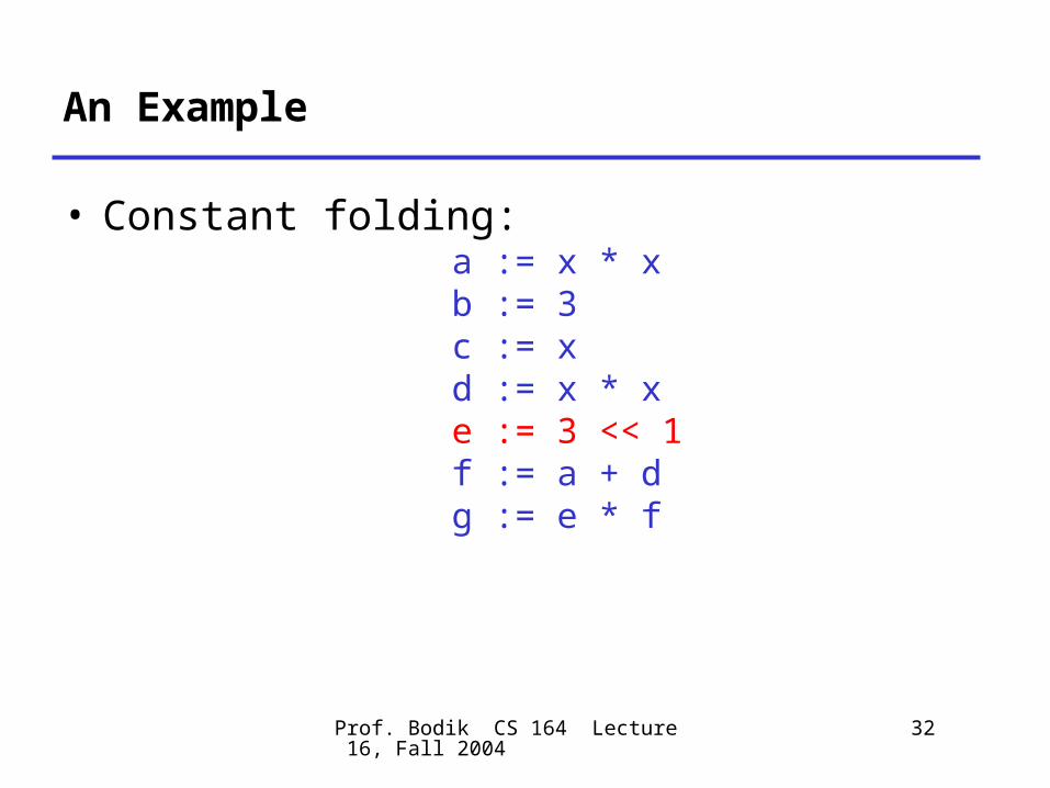
32

An Example

• Constant folding: a := x * x b := 3 c := x d := x * x e := 3 << 1 f := a + d g := e * f


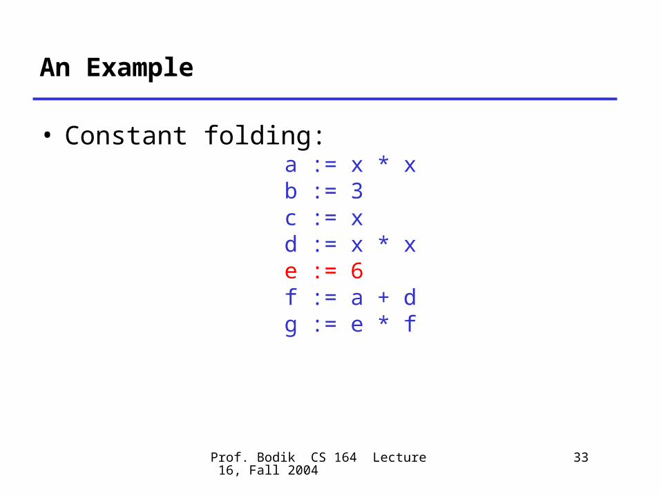
33

An Example

• Constant folding: a := x * x b := 3 c := x d := x * x e := 6 f := a + d g := e * f


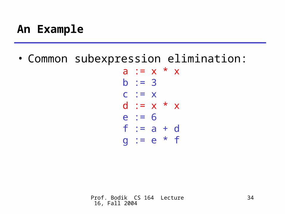
34

An Example

• Common subexpression elimination: a := x * x b := 3 c := x d := x * x e := 6 f := a + d g := e * f


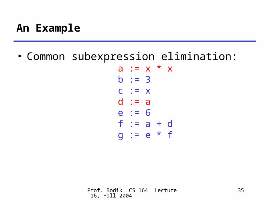
35

An Example

• Common subexpression elimination: a := x * x b := 3 c := x d := a e := 6 f := a + d g := e * f


36

An Example

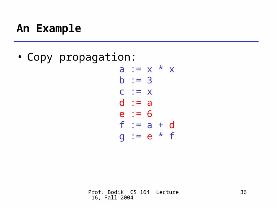
• Copy propagation: a := x * x b := 3 c := x d := a e := 6 f := a + d g := e * f


37

An Example

• Copy propagation: a := x * x b := 3 c := x d := a e := 6 f := a + a g := 6 * f


38

An Example

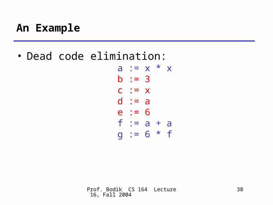
• Dead code elimination: a := x * x b := 3 c := x d := a e := 6 f := a + a g := 6 * f


39

An Example

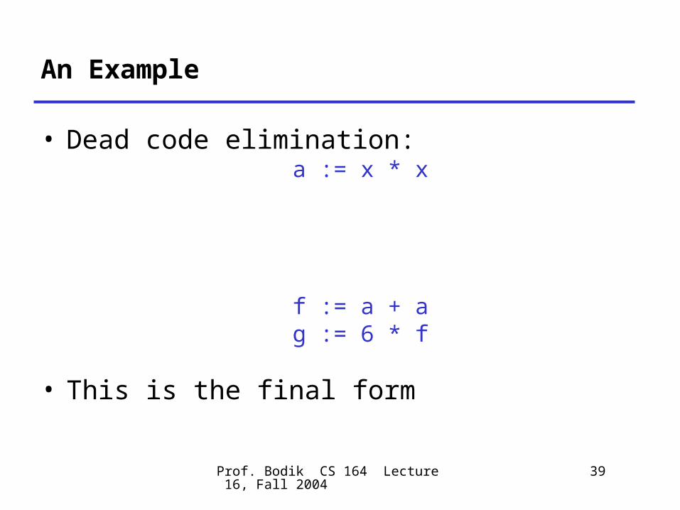
• Dead code elimination: a := x * x

f := a + a g := 6 * f

• This is the final form


40

Peephole Optimizations on Assembly Code

• The optimizations presented before work on intermediate code– They are target independent– But they can be applied on assembly language

also

• Peephole optimization is an effective technique for improving assembly code– The “peephole” is a short sequence of (usually

contiguous) instructions– The optimizer replaces the sequence with

another equivalent one (but faster)


41

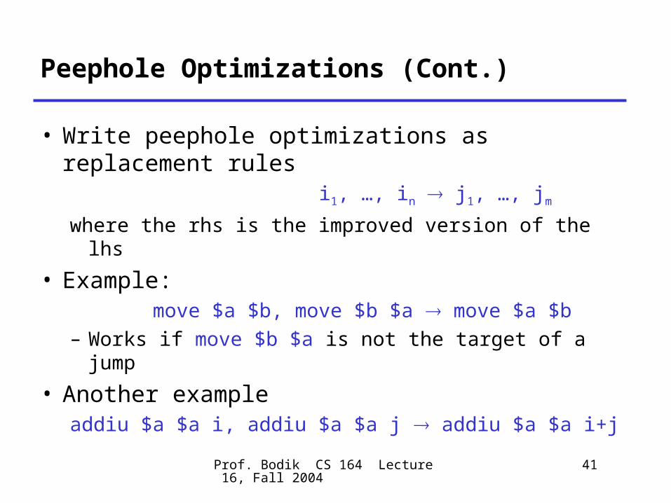
Peephole Optimizations (Cont.)

• Write peephole optimizations as replacement rules i1, …, in j1, …, jmwhere the rhs is the improved version of the lhs

• Example: move $a $b, move $b $a move $a $b– Works if move $b $a is not the target of a jump

• Another exampleaddiu $a $a i, addiu $a $a j addiu $a $a i+j


42

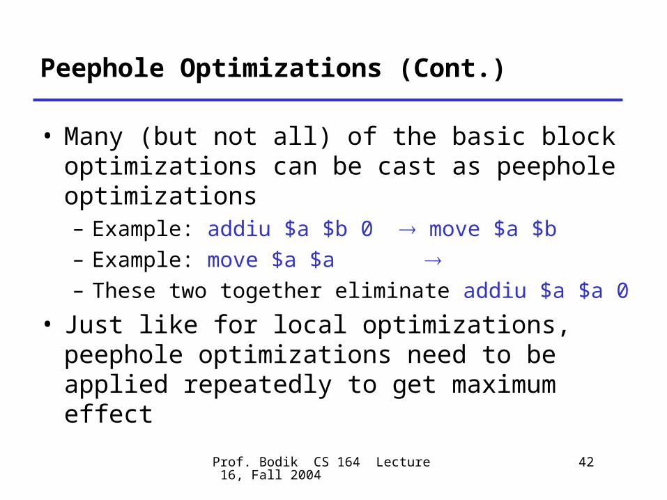
Peephole Optimizations (Cont.)

• Many (but not all) of the basic block optimizations can be cast as peephole optimizations– Example: addiu $a $b 0 move $a $b– Example: move $a $a – These two together eliminate addiu $a $a 0

• Just like for local optimizations, peephole optimizations need to be applied repeatedly to get maximum effect


43

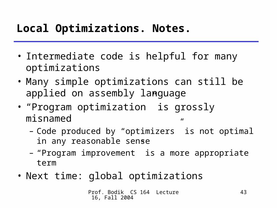
Local Optimizations. Notes.

• Intermediate code is helpful for many optimizations

• Many simple optimizations can still be applied on assembly language

• “Program optimization” is grossly misnamed– Code produced by “optimizers” is not optimal in

any reasonable sense– “Program improvement” is a more appropriate

term

• Next time: global optimizations

Documents

Prof. Bodik CS 164 Lecture 16, Fall 20041 Intermediate Code. Local Optimizations Lecture 15