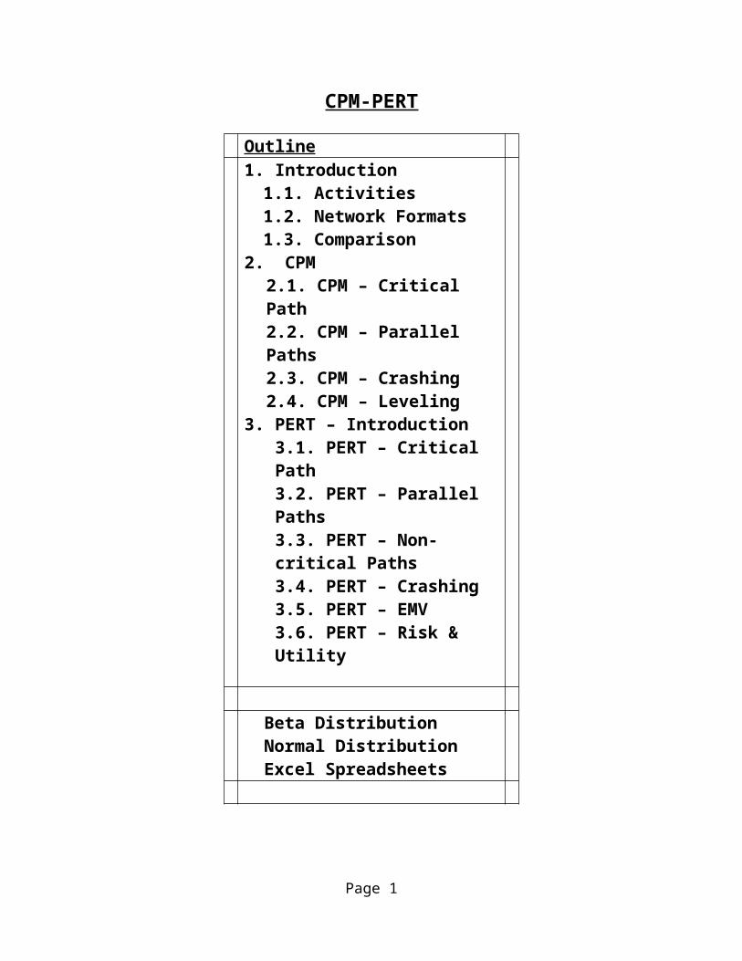
CPM-PERT

Outline1. Introduction

1.1. Activities1.2. Network Formats1.3. Comparison

2. CPM2.1. CPM – Critical Path2.2. CPM – Parallel Paths2.3. CPM – Crashing2.4. CPM – Leveling

3. PERT – Introduction3.1. PERT – Critical Path3.2. PERT – Parallel Paths3.3. PERT – Non-critical Paths3.4. PERT – Crashing3.5. PERT – EMV3.6. PERT – Risk & Utility

Beta DistributionNormal DistributionExcel Spreadsheets

Page 1

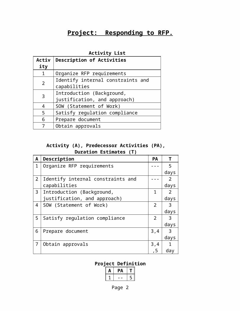
Project: Responding to RFP.

Activity ListActivit

yDescription of Activities

1 Organize RFP requirements2 Identify internal constraints and capabilities3 Introduction (Background, justification, and approach)4 SOW (Statement of Work)5 Satisfy regulation compliance6 Prepare document7 Obtain approvals

Activity (A), Predecessor Activities (PA), Duration Estimates (T)A Description PA T1 Organize RFP requirements --- 5 days2 Identify internal constraints and capabilities --- 2 days3 Introduction (Background, justification, and approach) 1 2 days4 SOW (Statement of Work) 2 3 days5 Satisfy regulation compliance 2 3 days6 Prepare document 3,4 3 days7 Obtain approvals 3,4,5 1 day

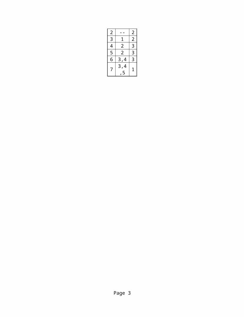
Project DefinitionA PA T1 -- 52 -- 23 1 24 2 35 2 36 3,4 3

7 3,4,5 1

Page 2

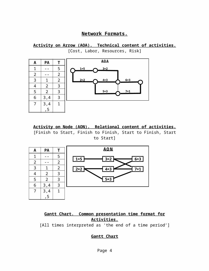
Network Formats.

Activity on Arrow (AOA). Technical content of activities.[Cost, Labor, Resources, Risk]

A PA T1 -- 52 -- 23 1 24 2 35 2 36 3,4 37 3,4,5 1

Activity on Node (AON). Relational content of activities.[Finish to Start, Finish to Finish, Start to Finish, Start to Start]

A PA T1 -- 52 -- 23 1 24 2 35 2 36 3,4 37 3,4,5 1

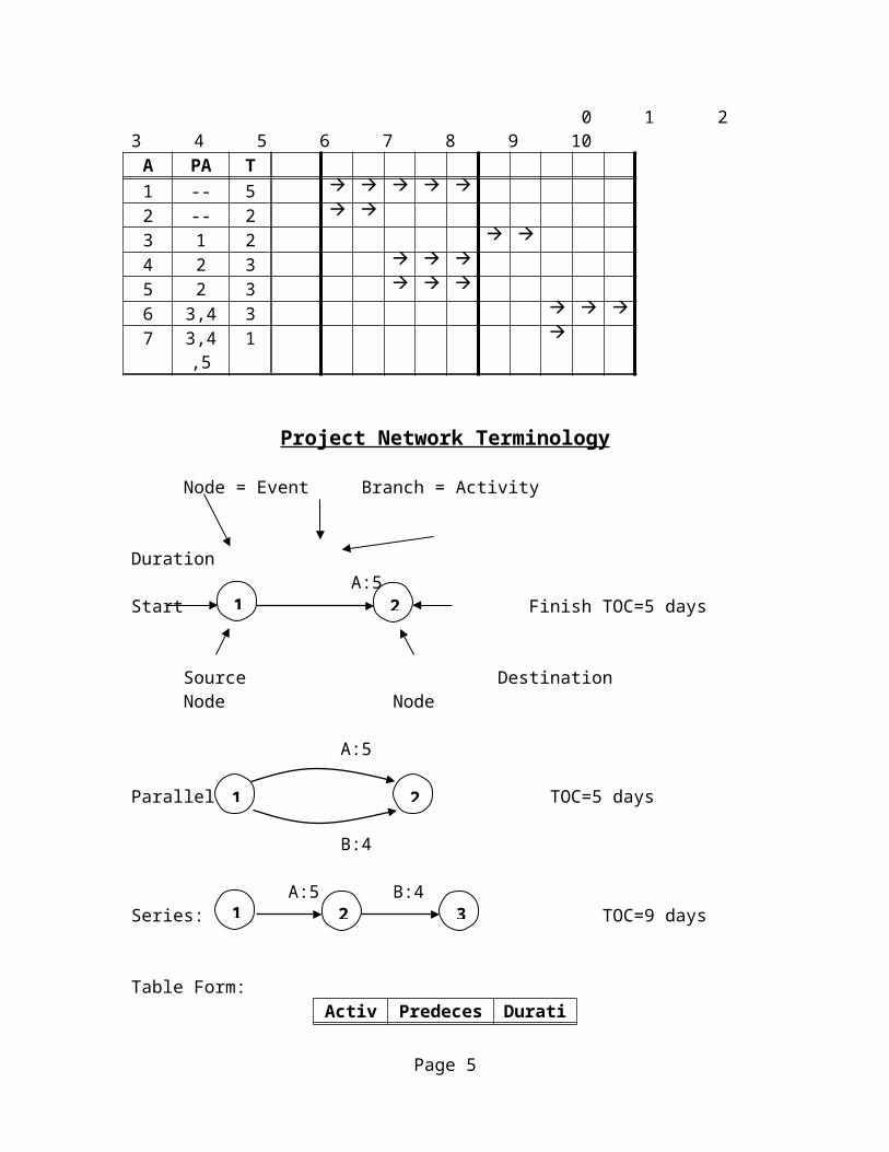
Gantt Chart. Common presentation time format for Activities.[All times interpreted as ‘the end of a time period’]

Gantt Chart 0 1 2 3 4 5 6 7 8 9 10

A PA T1 -- 5 2 -- 2 3 1 2 4 2 3 5 2 3 6 3,4 3 7 3,4,5 1

Page 3

AOA

1=5 3=2

2=2 4=3 6=3

5=3 7=1

AON

1=5 3=2 6=3

2=2 4=3 7=1

5=3

Project Network Terminology

Node = Event Branch = Activity

Duration A:5

Start Finish TOC=5 days

Source DestinationNode Node

A:5

Parallel: TOC=5 days

B:4

A:5 B:4Series: TOC=9 days

Table Form:

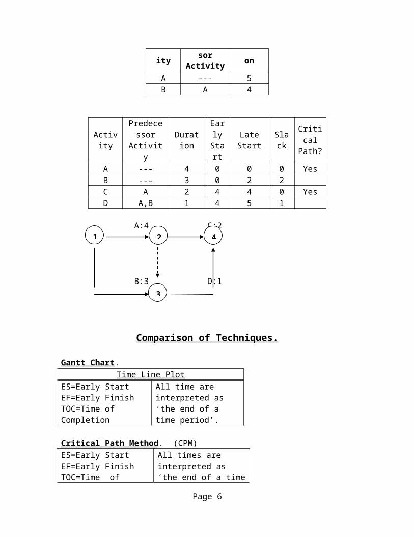
Activity PredecessorActivity Duration

A --- 5B A 4

ActivityPredecesso

rActivity

DurationEarl

yStart

Late Start Slack CriticalPath?

A --- 4 0 0 0 YesB --- 3 0 2 2C A 2 4 4 0 YesD A,B 1 4 5 1

A:4 C:2

B:3 D:1

Page 4

1 2

1 2

1 2

3

1

3

42

Comparison of Techniques.

Gantt Chart. Time Line Plot

ES=Early StartEF=Early FinishTOC=Time of Completion

All time are interpreted as‘the end of a time period’.

Critical Path Method. (CPM)ES=Early StartEF=Early FinishTOC=Time of CompletionLS=Late StartLF=Late FinishSlack= LF–EF=LS–ES

All times are interpreted as‘the end of a time period’

Slack=Total SlackA Critical Activity is an activity with zero slack.All critical activities define the Critical Path, CP.

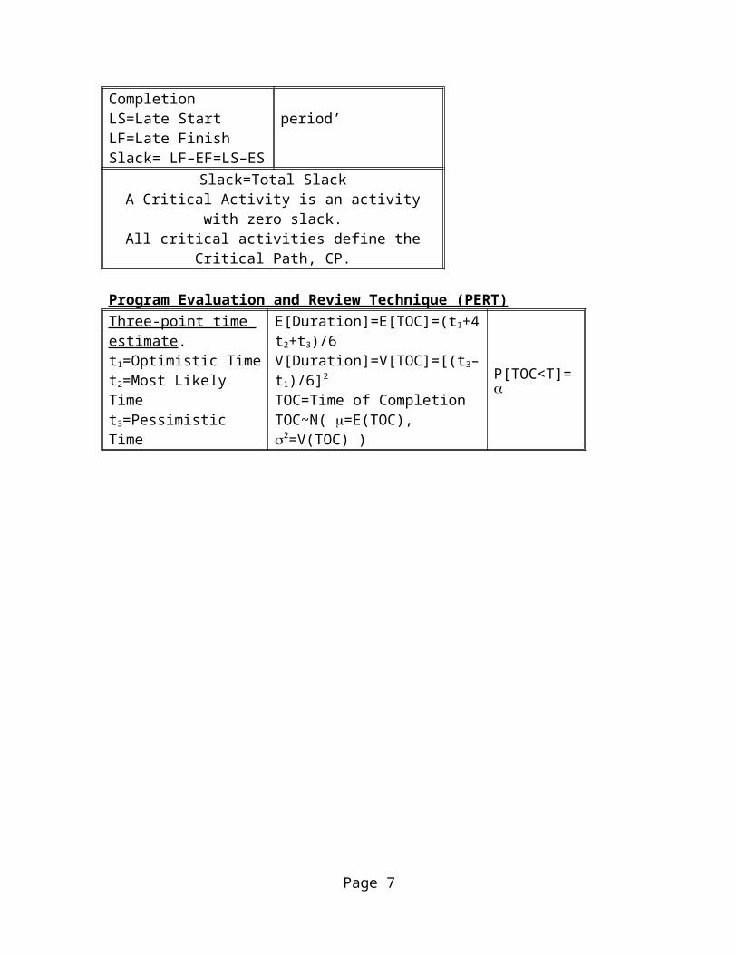
Program Evaluation and Review Technique (PERT)Three-point time estimate.t1=Optimistic Timet2=Most Likely Timet3=Pessimistic Time

E[Duration]=E[TOC]=(t1+4t2+t3)/6V[Duration]=V[TOC]=[(t3–t1)/6]2

TOC=Time of CompletionTOC~N( =E(TOC), 2=V(TOC) )

P[TOC<T]=

Page 5

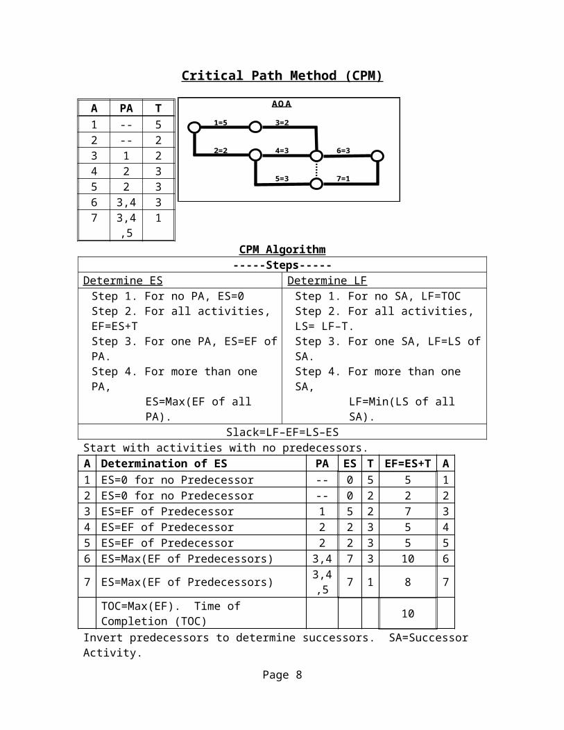
Critical Path Met hod (CPM)

A PA T1 -- 52 -- 23 1 24 2 35 2 36 3,4 37 3,4,5 1

CPM Algorithm-----Steps-----

Determine ES Determine LFStep 1. For no PA, ES=0Step 2. For all activities, EF=ES+TStep 3. For one PA, ES=EF of PA.Step 4. For more than one PA,

ES=Max(EF of all PA).

Step 1. For no SA, LF=TOCStep 2. For all activities, LS= LF–T.Step 3. For one SA, LF=LS of SA.Step 4. For more than one SA,

LF=Min(LS of all SA).Slack=LF–EF=LS–ES

Start with activities with no predecessors.

A Determination of ES PA ES T EF=ES+T A

1 ES=0 for no Predecessor -- 0 5 5 12 ES=0 for no Predecessor -- 0 2 2 23 ES=EF of Predecessor 1 5 2 7 34 ES=EF of Predecessor 2 2 3 5 45 ES=EF of Predecessor 2 2 3 5 56 ES=Max(EF of Predecessors) 3,4 7 3 10 67 ES=Max(EF of Predecessors) 3,4,5 7 1 8 7

TOC=Max(EF). Time of Completion (TOC) 10

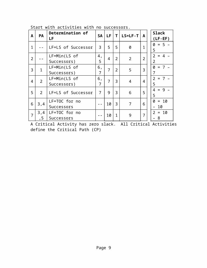
Invert predecessors to determine successors. SA=Successor Activity.Start with activities with no successors.

A PA Determination of LF SA LF T LS=LF–T A Slack(LF–EF)

1 -- LF=LS of Successor 3 5 5 0 1 0 = 5 – 52 -- LF=Min(LS of Successors) 4,5 4 2 2 2 2 = 4 – 23 1 LF=Min(LS of Successors) 6,7 7 2 5 3 0 = 7 – 74 2 LF=Min(LS of Successors) 6,7 7 3 4 4 2 = 7 – 55 2 LF=LS of Successor 7 9 3 6 5 4 = 9 – 56 3,4 LF=TOC for no Successors -- 10 3 7 6 0 = 10 – 107 3,4,5 LF=TOC for no Successors -- 10 1 9 7 2 = 10 – 8A Critical Activity has zero slack. All Critical Activities define the Critical Path (CP)

Page 6

AOA

1=5 3=2

2=2 4=3 6=3

5=3 7=1

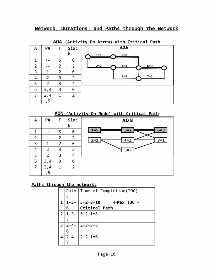
Network, Durations, and Paths through the Network

AOA (Activity On Arrow) with Critical Path A PA T Slack

1 -- 5 02 -- 2 23 1 2 04 2 3 25 2 3 46 3,4 3 07 3,4,5 1 2

AON (Activity On Node) with Critical Path A PA T Slack

1 -- 5 02 -- 2 23 1 2 04 2 3 25 2 3 46 3,4 3 07 3,4,

51 2

Paths through the network:Paths: Time of Completion(TOC)

1 1-3-6 5+2+3=10 Max TOC = Critical Path

2 1-3-7 5+2+1=83 2-4-6 2+3+3=84 2-4-7 2+3+1=6

Page 7

AON

1=5 3=2 6=3

2=2 4=3 7=1

5=3

AOA

1=5 3=2

2=2 4=3 6=3

5=3 7=1

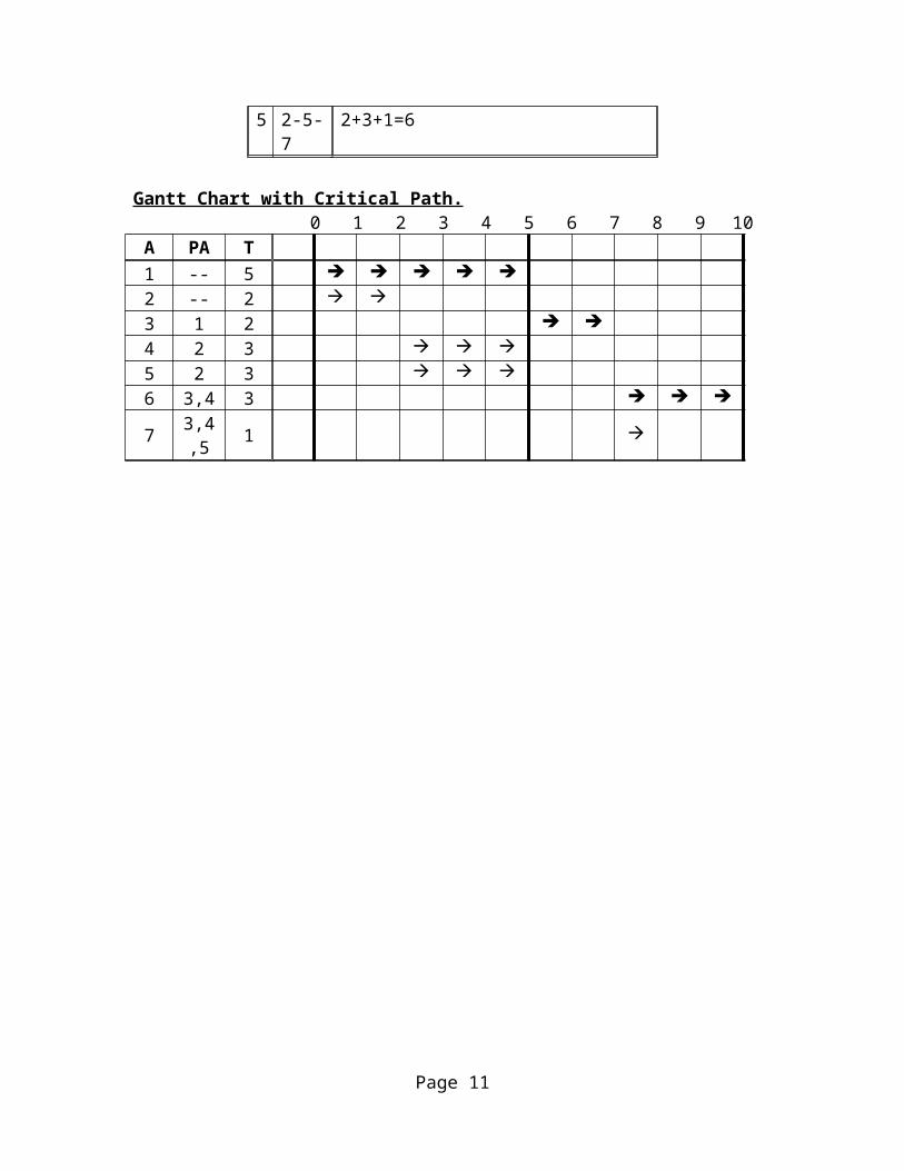
5 2-5-7 2+3+1=6

Gantt Chart with Critical Path.0 1 2 3 4 5 6 7 8 9 10

A PA T1 -- 5 2 -- 2 3 1 2 4 2 3 5 2 3 6 3,4 3 7 3,4,5 1

Page 8

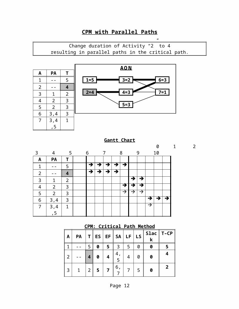
CPM with Parallel Paths

Change duration of Activity “2” to 4resulting in parallel paths in the critical path.

A PA T1 -- 52 -- 43 1 24 2 35 2 36 3,4 37 3,4,5 1

Gantt Chart 0 1 2 3 4 5 6 7 8 9 10

A PA T1 -- 5 2 -- 4 3 1 2 4 2 3 5 2 3 6 3,4 3 7 3,4,5 1

CPM: Critical Path Method

A PA T ES EF SA LF LS Slack T–CP

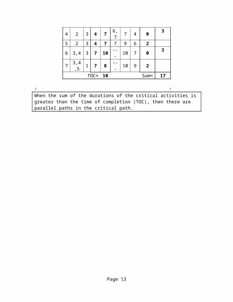
1 -- 5 0 5 3 5 0 0 52 -- 4 0 4 4,5 4 0 0 43 1 2 5 7 6,7 7 5 0 24 2 3 4 7 6,7 7 4 0 35 2 3 4 7 7 9 6 26 3,4 3 7 10 --- 10 7 0 37 3,4,5 1 7 8 --- 10 9 2

TOC= 10 Sum= 17 ↑ ↑When the sum of the durations of the critical activities is greater than the time of completion (TOC), then there are parallel paths in the critical path.

Page 9

AON

1=5 3=2 6=3

2=4 4=3 7=1

5=3

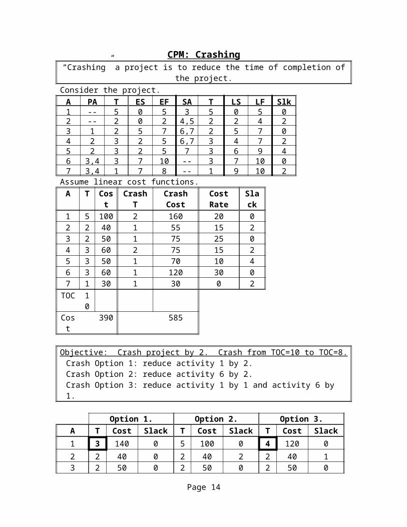
CPM: Crashing“Crashing” a project is to reduce the time of completion of the project.

Consider the project.A PA T ES EF SA T LS LF Slk1 -- 5 0 5 3 5 0 5 02 -- 2 0 2 4,5 2 2 4 23 1 2 5 7 6,7 2 5 7 04 2 3 2 5 6,7 3 4 7 25 2 3 2 5 7 3 6 9 46 3,4 3 7 10 -- 3 7 10 07 3,4,5 1 7 8 -- 1 9 10 2

Assume linear cost functions.A T Cost Crash T Crash Cost Cost Rate Slack1 5 100 2 160 20 02 2 40 1 55 15 23 2 50 1 75 25 04 3 60 2 75 15 25 3 50 1 70 10 46 3 60 1 120 30 07 1 30 1 30 0 2

TOC

10

Cost 390 585

Objective: Crash project by 2. Crash from TOC=10 to TOC=8.Crash Option 1: reduce activity 1 by 2.Crash Option 2: reduce activity 6 by 2.Crash Option 3: reduce activity 1 by 1 and activity 6 by 1.

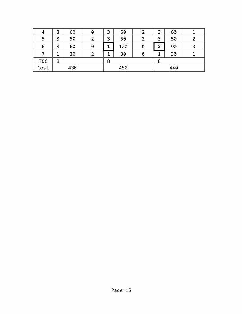
Option 1. Option 2. Option 3.A T Cost Slack T Cost Slack T Cost Slack1 3 140 0 5 100 0 4 120 02 2 40 0 2 40 2 2 40 13 2 50 0 2 50 0 2 50 04 3 60 0 3 60 2 3 60 15 3 50 2 3 50 2 3 50 26 3 60 0 1 120 0 2 90 07 1 30 2 1 30 0 1 30 1

TOC 8 8 8Cost 430 450 440

Page 10

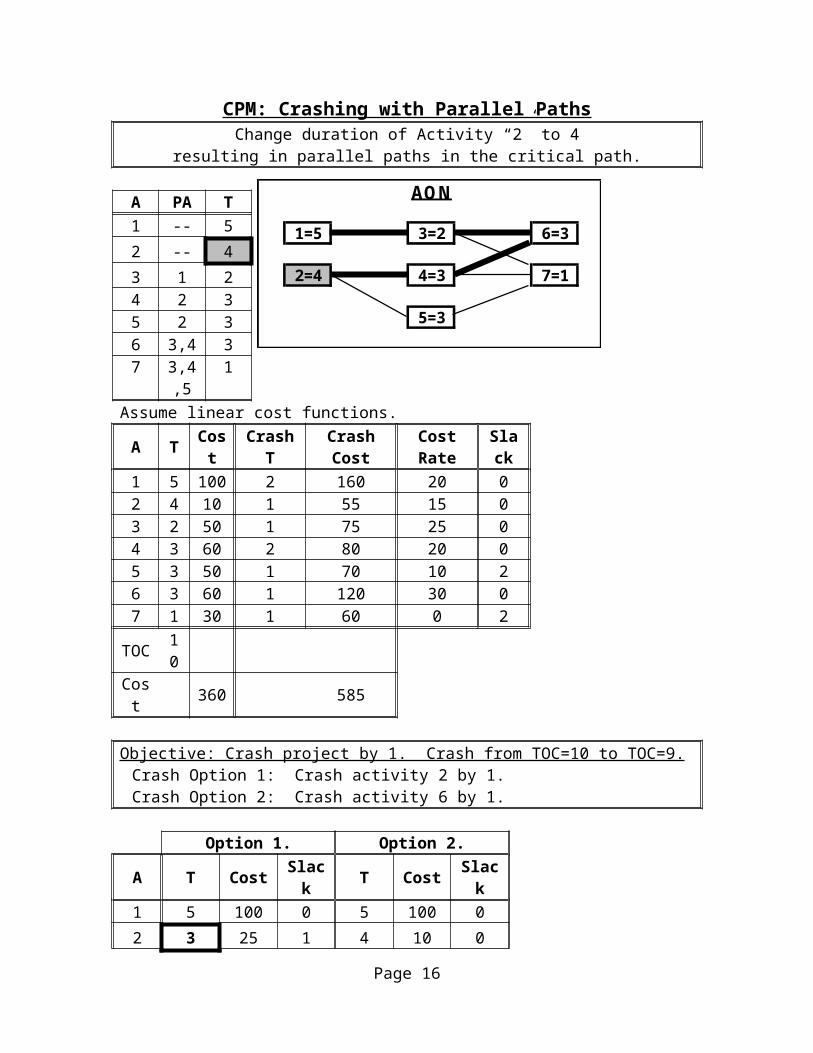
CPM: Crashing with Parallel PathsChange duration of Activity “2” to 4

resulting in parallel paths in the critical path.

A PA T1 -- 52 -- 43 1 24 2 35 2 36 3,4 37 3,4,5 1

Assume linear cost functions.A T Cost Crash T Crash Cost Cost Rate Slack1 5 100 2 160 20 02 4 10 1 55 15 03 2 50 1 75 25 04 3 60 2 80 20 05 3 50 1 70 10 26 3 60 1 120 30 07 1 30 1 60 0 2

TOC 10

Cost 360 585

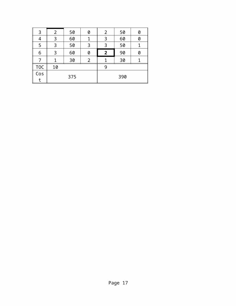
Objective: Crash project by 1. Crash from TOC=10 to TOC=9.Crash Option 1: Crash activity 2 by 1.Crash Option 2: Crash activity 6 by 1.

Option 1. Option 2.A T Cost Slack T Cost Slack1 5 100 0 5 100 02 3 25 1 4 10 03 2 50 0 2 50 04 3 60 1 3 60 05 3 50 3 3 50 16 3 60 0 2 90 07 1 30 2 1 30 1

TOC 10 9Cost 375 390

Page 11

AON

1=5 3=2 6=3

2=4 4=3 7=1

5=3

Page 12

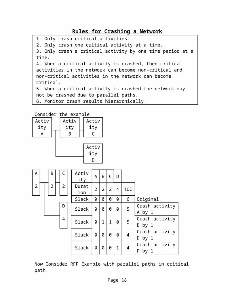
Rules for Crashing a Network1. Only crash critical activities.2. Only crash one critical activity at a time.3. Only crash a critical activity by one time period at a time.4. When a critical activity is crashed, then critical activities in the network can become non-critical and non-critical activities in the network can become critical.5. When a critical activity is crashed the network may not be crashed due to parallel paths.6. Monitor crash results hierarchically.

Consider the example.

Activity Activity Activity

A B C

ActivityD

A B C Activity A B C D2 2 2 Duration 2 2 2 4 TOC

Slack 0 0 0 0 6 OriginalD Slack 0 0 0 0 5 Crash activity A by 14 Slack 0 1 1 0 5 Crash activity B by 1

Slack 0 0 0 0 4 Crash activity D by 1Slack 0 0 0 1 4 Crash activity D by 1

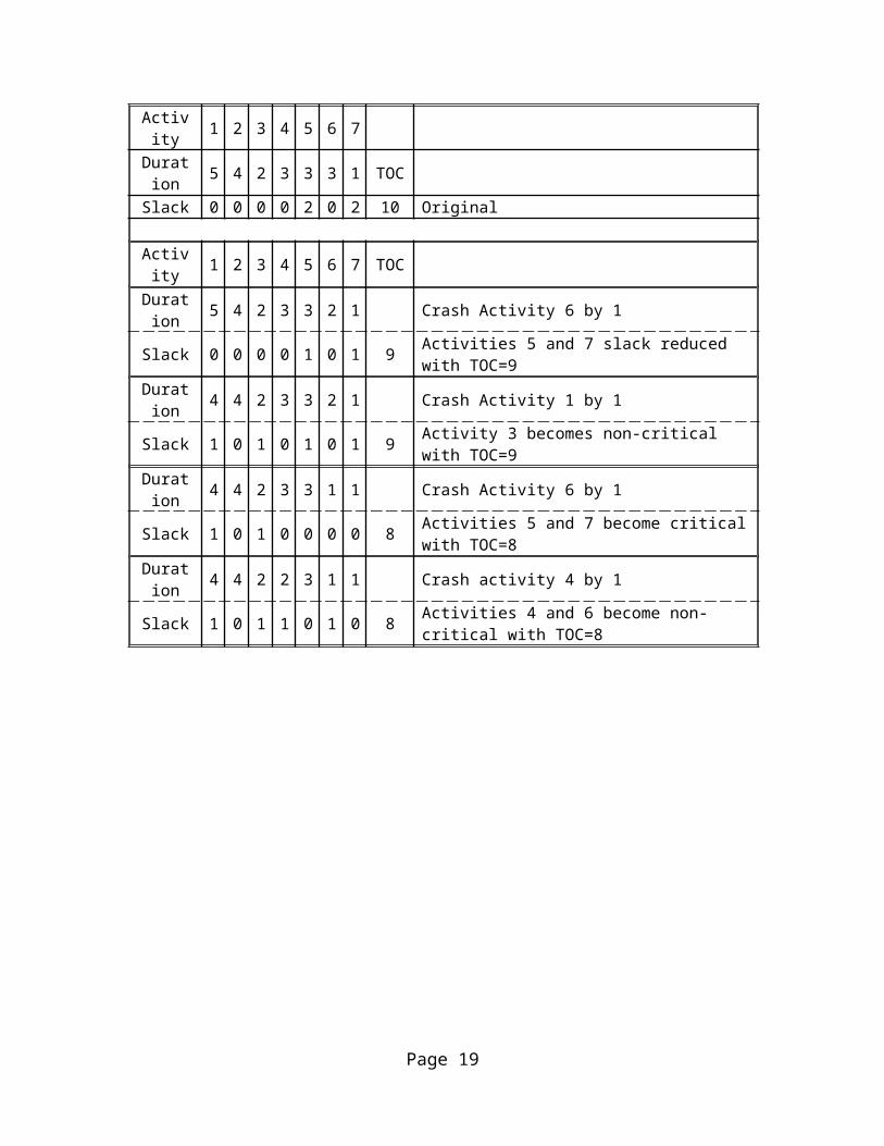
Now Consider RFP Example with parallel paths in critical path.Activity 1 2 3 4 5 6 7Duration 5 4 2 3 3 3 1 TOC

Slack 0 0 0 0 2 0 2 10 Original

Activity 1 2 3 4 5 6 7 TOCDuration 5 4 2 3 3 2 1 Crash Activity 6 by 1

Slack 0 0 0 0 1 0 1 9 Activities 5 and 7 slack reduced with TOC=9Duration 4 4 2 3 3 2 1 Crash Activity 1 by 1

Slack 1 0 1 0 1 0 1 9 Activity 3 becomes non-critical with TOC=9Duration 4 4 2 3 3 1 1 Crash Activity 6 by 1

Slack 1 0 1 0 0 0 0 8 Activities 5 and 7 become critical with TOC=8Duration 4 4 2 2 3 1 1 Crash activity 4 by 1

Slack 1 0 1 1 0 1 0 8 Activities 4 and 6 become non-critical with TOC=8

Page 13

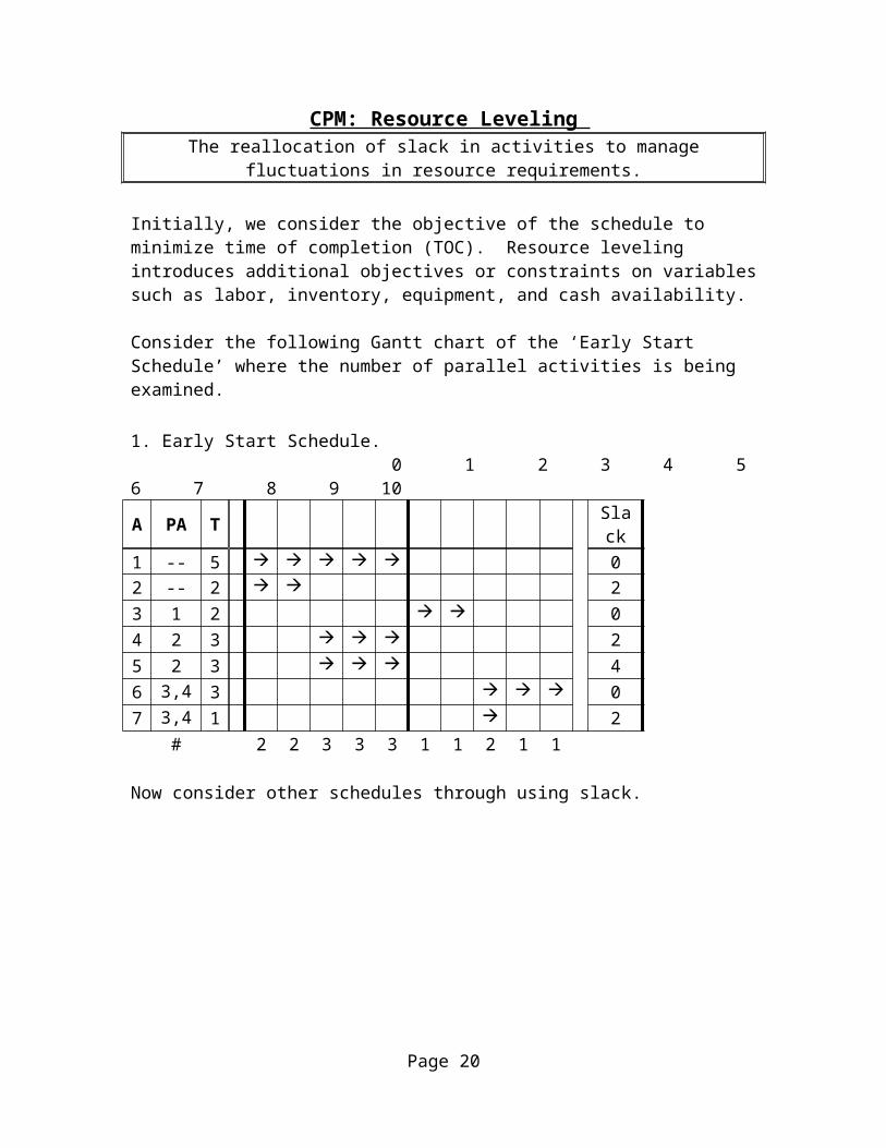
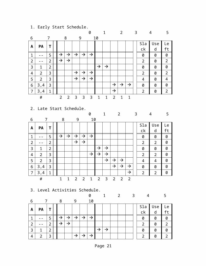
CPM: Resource Leveling The reallocation of slack in activities to manage fluctuations in resource requirements.

Initially, we consider the objective of the schedule to minimize time of completion (TOC). Resource leveling introduces additional objectives or constraints on variables such as labor, inventory, equipment, and cash availability.

Consider the following Gantt chart of the ‘Early Start Schedule’ where the number of parallel activities is being examined.

1. Early Start Schedule. 0 1 2 3 4 5 6 7 8 9 10A PA T Slack1 -- 5 02 -- 2 23 1 2 04 2 3 25 2 3 46 3,4 3 07 3,4,5 1 2

# 2 2 3 3 3 1 1 2 1 1

Now consider other schedules through using slack.

Page 14

1. Early Start Schedule. 0 1 2 3 4 5 6 7 8 9 10A PA T Slack Used Left1 -- 5 0 0 02 -- 2 2 0 2

3 1 2 0 0 0

4 2 3 2 0 2

5 2 3 4 0 4

6 3,4 3 0 0 0

7 3,4,5

1 2 0 2

# 2 2 3 3 3 1 1 2 1 1

2. Late Start Schedule. 0 1 2 3 4 5 6 7 8 9 10A PA T Slack Used Left1 -- 5 0 0 02 -- 2 2 2 0

3 1 2 0 0 0

4 2 3 2 2 0

5 2 3 4 4 0

6 3,4 3 0 0 0

7 3,4,5

1 2 2 0

# 1 1 2 2 1 2 3 2 2 2

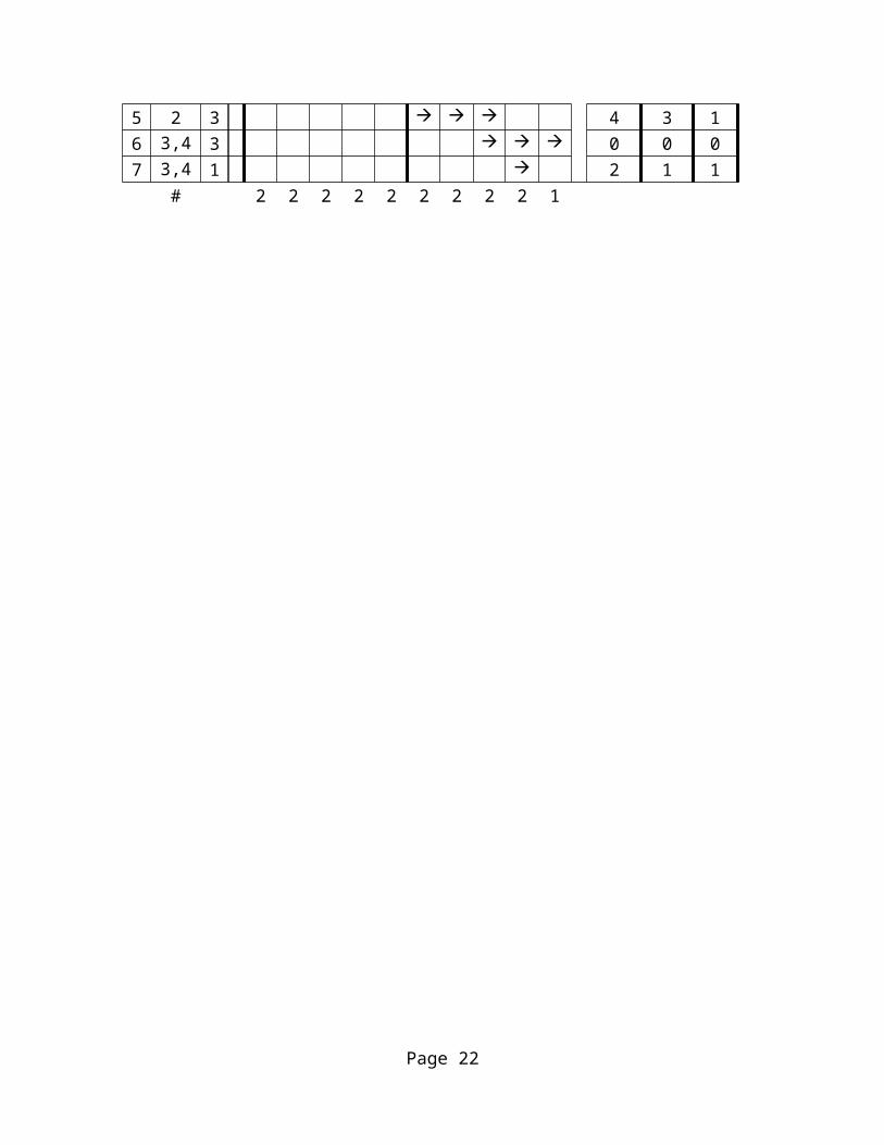
3. Level Activities Schedule. 0 1 2 3 4 5 6 7 8 9 10A PA T Slack Used Left1 -- 5 0 0 02 -- 2 2 0 23 1 2 0 0 04 2 3 2 0 25 2 3 4 3 16 3,4 3 0 0 07 3,4,

51 2 1 1

# 2 2 2 2 2 2 2 2 2 1

Page 15

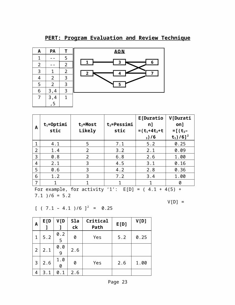
PERT: Program Evaluation and Review Technique

A PA T

1 -- 52 -- 23 1 24 2 35 2 36 3,4 37 3,4,5 1

A t1=Optimistic t2=Most Likely t3=Pessimistic E[Duration]=(t1+4t2+t3)/6

V[Duration]=[(t3–t1)/6]2

1 4.1 5 7.1 5.2 0.252 1.4 2 3.2 2.1 0.093 0.8 2 6.8 2.6 1.004 2.1 3 4.5 3.1 0.165 0.6 3 4.2 2.8 0.366 1.2 3 7.2 3.4 1.007 1 1 1 1 0For example, for activity ‘1’: E[D] = ( 4.1 + 4(5) + 7.1 )/6 = 5.2 V[D] = [ ( 7.1 – 4.1 )/6 ]2 = 0.25

A E[D] V[D] Slack Critical Path E[D] V[D]

1 5.2 0.25 0 Yes 5.2 0.252 2.1 0.09 2.63 2.6 1.00 0 Yes 2.6 1.004 3.1 0.16 2.65 2.8 0.36 5.36 3.4 1.00 0 Yes 3.4 1.007 1 0 2.4

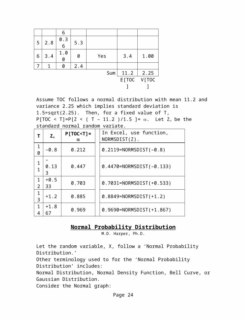
Sum 11.2 2.25E[TOC] V[TOC]

Page 16

AON

1 3 6

2 4 7

5

Assume TOC follows a normal distribution with mean 11.2 and variance 2.25 which implies standard deviation is 1.5=sqrt(2.25). Then, for a fixed value of T, P[TOC < T]=P[Z < ( T – 11.2 )/1.5 ]= . Let Z be the standard normal random variate. T Z P[TOC<T]= In Excel, use function, NORMSDIST(Z).10 –0.8 0.212 0.2119=NORMSDIST(–0.8)11 –0.133 0.447 0.4470=NORMSDIST(–0.133)

12 +0.533 0.703 0.7031=NORMSDIST(+0.533)

13 +1.2 0.885 0.8849=NORMSDIST(+1.2)

14 +1.867 0.969 0.9690=NORMSDIST(+1.867)

Normal Probability DistributionM.D. Harper, Ph.D.

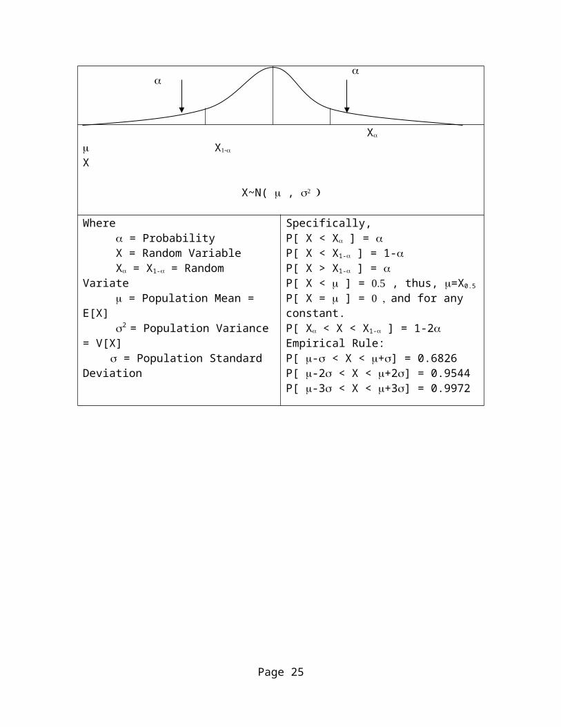
Let the random variable, X, follow a ‘Normal Probability Distribution.’Other terminology used to for the ‘Normal Probability Distribution’ includes:Normal Distribution, Normal Density Function, Bell Curve, or Gaussian Distribution.Consider the Normal graph:

X X X

X~N( ,

Where = Probability X = Random Variable X = X1- = Random Variate = Population Mean = E[X] 2 = Population Variance = V[X] = Population Standard Deviation

Specifically,P[ X < X ] = P[ X < X1- ] = 1-P[ X > X1- ] = P[ X < ] = , thus, =X0.5

P[ X = ] = and for any constant.P[ X < X < X1- ] = 1-2Empirical Rule:P[ - < X < +] = 0.6826P[ -2 < X < +2] = 0.9544P[ -3 < X < +3] = 0.9972

Page 17

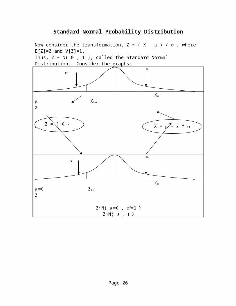
Standard Normal Probability Distribution

Now consider the transformation, Z = ( X - ) / , where E[Z]=0 and V[Z]=1.Thus, Z ~ N( 0 , 1 ), called the Standard Normal Distribution. Consider the graphs:

X X X

X~N( ,

Z Z Z

Z~N( , =1Z~N( ,

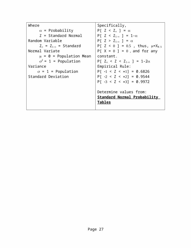
Where = Probability Z = Standard Normal Random Variable Z = Z1- = Standard Normal Variate = 0 = Population Mean 2 = 1 = Population Variance = 1 = Population Standard Deviation

Specifically,P[ Z < Z ] = P[ Z < Z1- ] = 1-P[ Z > Z1- ] = P[ Z < ] = , thus, =X0.5

P[ X = ] = and for any constant.P[ Z < Z < Z1- ] = 1-2Empirical Rule:P[ < Z < ] = 0.6826P[ < Z < ] = 0.9544P[ < Z < ] = 0.9972

Determine values from:Standard Normal Probability Tables

Page 18

Z = ( X - ) / X = + Z *

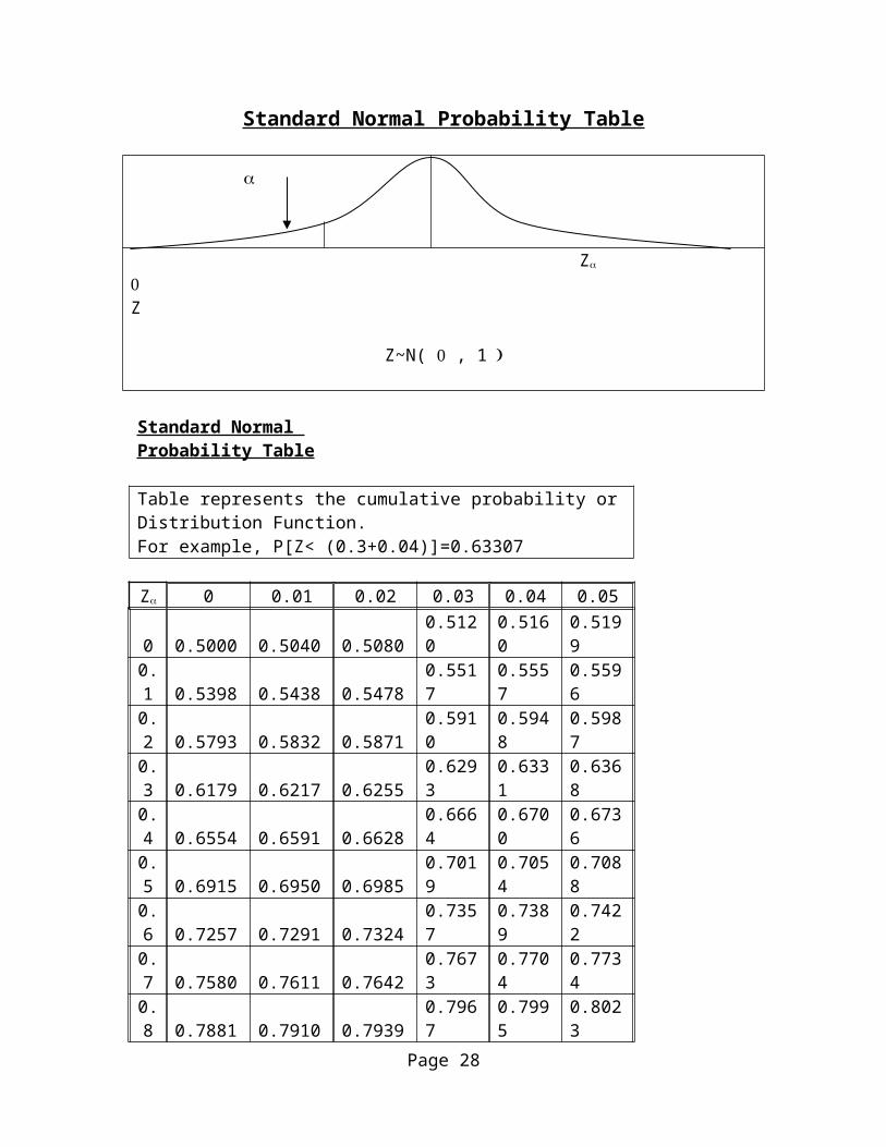
Standard Normal Probability Table

Z Z

Z~N( , 1

Standard Normal Probability Table

Table represents the cumulative probability or Distribution Function.For example, P[Z< (0.3+0.04)]=0.63307

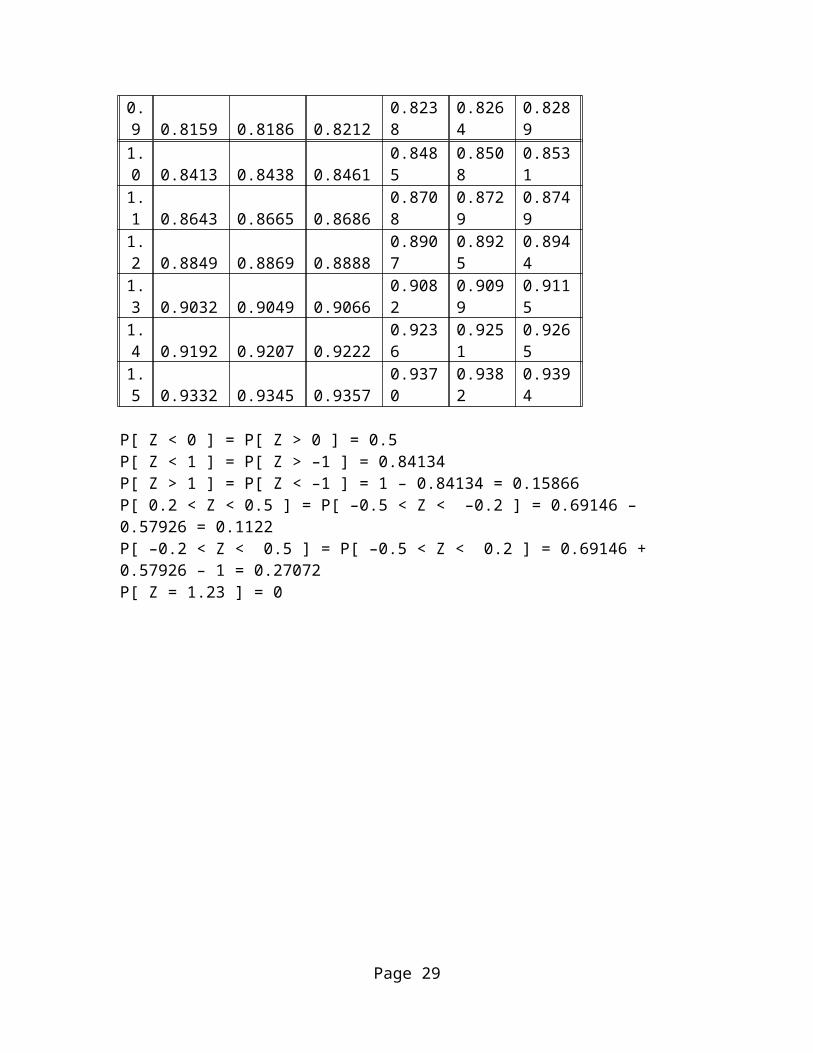
Z 0 0.01 0.02 0.03 0.04 0.050 0.5000 0.5040 0.5080 0.5120 0.5160 0.51990.1 0.5398 0.5438 0.5478 0.5517 0.5557 0.55960.2 0.5793 0.5832 0.5871 0.5910 0.5948 0.59870.3 0.6179 0.6217 0.6255 0.6293 0.6331 0.63680.4 0.6554 0.6591 0.6628 0.6664 0.6700 0.67360.5 0.6915 0.6950 0.6985 0.7019 0.7054 0.70880.6 0.7257 0.7291 0.7324 0.7357 0.7389 0.74220.7 0.7580 0.7611 0.7642 0.7673 0.7704 0.77340.8 0.7881 0.7910 0.7939 0.7967 0.7995 0.80230.9 0.8159 0.8186 0.8212 0.8238 0.8264 0.82891.0 0.8413 0.8438 0.8461 0.8485 0.8508 0.85311.1 0.8643 0.8665 0.8686 0.8708 0.8729 0.87491.2 0.8849 0.8869 0.8888 0.8907 0.8925 0.89441.3 0.9032 0.9049 0.9066 0.9082 0.9099 0.9115

Page 19

1.4 0.9192 0.9207 0.9222 0.9236 0.9251 0.92651.5 0.9332 0.9345 0.9357 0.9370 0.9382 0.9394

P[ Z < 0 ] = P[ Z > 0 ] = 0.5P[ Z < 1 ] = P[ Z > –1 ] = 0.84134P[ Z > 1 ] = P[ Z < –1 ] = 1 – 0.84134 = 0.15866P[ 0.2 < Z < 0.5 ] = P[ –0.5 < Z < –0.2 ] = 0.69146 – 0.57926 = 0.1122P[ –0.2 < Z < 0.5 ] = P[ –0.5 < Z < 0.2 ] = 0.69146 + 0.57926 – 1 = 0.27072P[ Z = 1.23 ] = 0

Page 20

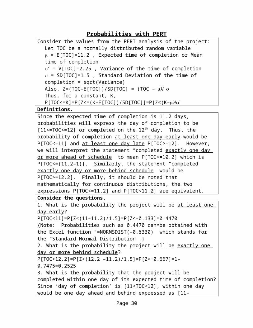
Probabilities with PERTConsider the values from the PERT analysis of the project:

Let TOC be a normally distributed random variable = E[TOC]=11.2 , Expected time of completion or Mean time of completion2 = V[TOC]=2.25 , Variance of the time of completion = SD[TOC]=1.5 , Standard Deviation of the time of completion = sqrt(Variance)Also, Z=(TOC–E[TOC])/SD[TOC] = (TOC –Thus, for a constant, K, P[TOC<=K]=P[Z<=(K–E[TOC])/SD[TOC]]=P[Z<(K–

Definitions.Since the expected time of completion is 11.2 days, probabilities will express the day of completion to be [11<=TOC<=12] or completed on the 12th day. Thus, the probability of completion at least one day early would be P[TOC<=11] and at least one day late P[TOC>=12]. However, we will interpret the statement “completed exactly one day or more ahead of schedule” to mean P[TOC<=10.2] which is P[TOC<=(11.2–1)]. Similarly, the statement “completed exactly one day or more behind schedule” would be P[TOC>=12.2]. Finally, it should be noted that mathematically for continuous distributions, the two expressions P[TOC<=11.2] and P[TOC<11.2] are equivalent.Consider the questions.1. What is the probability the project will be at least one day early?P[TOC<11]=P[Z<(11–11.2)/1.5]=P[Z<–0.133]=0.4470{Note: Probabilities such as 0.4470 can be obtained with the Excel function “=NORMSDIST(–0.1330)” which stands for the “Standard Normal Distribution”.}2. What is the probability the project will be exactly one day or more behind schedule?P[TOC>12.2]=P[Z>(12.2 –11.2)/1.5]=P[Z>+0.667]=1–0.7475=0.25253. What is the probability that the project will be completed within one day of its expected time of completion? Since ‘day of completion’ is [11<TOC<12], within one day would be one day ahead and behind expressed as [11–1<TOC<12+1]. Thus,P[10<TOC<13]=P[(10–11.2)/1.5<Z<(13–11.2)/1.5]= P[–0.8<Z<+1.2] =P[Z<+1.2] – P[Z<–0.8]=0.8849–0.2119=0.6731

Random Variates with PERTFor a constant, K, consider the relations, P[TOC<=K]=P[Z<(K–= and P[Z<Z]=Equating the random variates and solving yields, K= + Z * Common Standard Normal Variates, Z , are

0.9 0.95 0.975 0.99 0.8413 0.9332 0.977

2 0.9938 0.9987

Z 1.2821.64

5 1.960 2.326 1.0 1.5 2.0 2.5 3.0

Consider the problems.1. What time of completion yields a 90% probability of meeting and a 10% probability of exceeding? TOC0.9= + Z * days2. What is a 90% confidence interval of the time of completion?(TOC0.05 , TOC0.95 )=(–3. What confidence results in an interval of mean plus or minus two standard deviations?Level of confidence =(2–1)=(2*0.9772–1)=0.9544. A 95.44% confidence interval.

Page 21

Page 22

PERT with Parallel PathsChange Duration Estimates of Activity 5.

A PA1 --2 --3 14 25 26 3,47 3,4,5

A t1=Optimistic t2=Most Likely t3=Pessimistic E[Duration]=(t1+4t2+t3)/6

V[Duration]=[(t3–t1)/6]2

1 4.1 5 7.1 5.2 0.252 1.4 2 3.2 2.1 0.093 0.8 2 6.8 2.6 1.004 2.1 3 4.5 3.1 0.165 5.2 7 15.4 8.1 2.896 1.2 3 7.2 3.4 1.007 1 1 1 1 0

Critical PathPath 1-3-6 Path 2-5-7

A E[D] V[D] Slack E[D] V[D] E[D

]V[D]

1 5.2 0.25 0 5.2 0.252 2.1 0.09 0 2.1 0.093 2.6 1.00 0 2.6 1.00

4 3.1 0.16 2.6 Non-Critical

5 8.1 2.89 0 8.1 2.896 3.4 1.00 0 3.4 1.007 1 0 0 1 0

Sum 11.2 2.25 11.2 2.98

T=Day: 9 10 11 11.2 12 13 14

Z136 -1.467-

0.800 -0.1330

0.533 1.200 1.867P[TOC136 < T]= 0.071 0.212 0.447 0.5 0.703 0.885 0.969

Z257 -1.274-

0.695 -0.1160

0.463 1.043 1.622P[TOC257 < T]= 0.101 0.243 0.454 0.5 0.678 0.851 0.948

P[TOC < T]= 0.007 0.052 0.203 0.25 0.477 0.753 0.918

Page 23

AON

1 3 6

2 4 7

5

Page 24

Non-critical Activities in PERT with Parallel PathsConsider in more detail how the project can be delayed beyond TOC.

1. All activities are stochastic except activity “7”.2. All activities are critical except activity “4”.3. Critical Path consists of activities 1,3,6, & 2,5,7.4. TOC is based on the mean duration of the critical activities.5. Assume probability of exceeding TOC due to path “1,3,6” is 0.56. Assume probability of exceeding TOC due to path “2,5,7” is 0.57. Since only activity “4” is non-critical, consider the paths:

1-3-62-4-6

1-3-72-4-7

2-5-72-4-7

8. If the duration of activities “2” & “4” exceed “1” & “3”, the project exceeds TOC.9. If the duration of activity “4” exceeds activity “5”, the project exceeds TOC.10. Assume probability of not exceeding TOC due to “2,4” exceeding “1,3” is P[T2+T4<(5.2+2.6)]=P[Z<( (5.2+2.6) – (2.1+3.1) )/sqrt(0.09+0.16) ) ] = 2 ≈ 111. Assume probability of not exceeding TOC due to “4” exceeding “5” is P[T4<8.1]=P[Z<( (8.1–3.1)/sqrt(0.16) ) ] = 1 ≈ 112. Therefore, the probability of not exceeding TOC is (0.5*0.5*1*2) = 0.25CAUTION: As variances increase for any activity or as the mean duration of non-critical activities increase, the probability will decrease.

A PA

Consider Paths:1-3-61-3-72-4-62-4-72-5-7

1 --2 --3 14 25 26 3,47 3,4,5

Critical PathPath 1-3-6 Path 2-5-7

A E[D] V[D] Slack E[D] V[D] E[D

]V[D]

1 5.2 0.25 0 5.2 0.252 2.1 0.09 0 2.1 0.093 2.6 1.00 0 2.6 1.004 3.1 0.16 2.6 Non-

Page 25

AON

1 3 6

2 4 7

5

Critical5 8.1 2.89 0 8.1 2.896 3.4 1.00 0 3.4 1.007 1 0 0 1 0

Sum 11.2 2.25 11.2 2.98Note: A complete analysis would include all conditions and paths.

Page 26

PERT Analysis of Critical and Non-critical Paths

8 9 10 11 12 13 14 15 160.0

0.2

0.4

0.6

0.8

1.0

1.2

Path"1-3-6"

Path "2-5-7"

Critical Path

T

P[ T

OC

<=

T ]

T=Day: 9 10 11 11.2 12 13 14

Z136 -1.467-

0.800 -0.1330

0.533 1.200 1.867P[TOC136 < T]= 0.071 0.212 0.447 0.5 0.703 0.885 0.969

Z257 -1.274-

0.695 -0.1160

0.463 1.043 1.622P[TOC257 < T]= 0.101 0.243 0.454 0.5 0.678 0.851 0.948

P[TOC < T]= 0.007 0.052 0.203 0.25 0.477 0.753 0.918

1 2 3 4 5 6 7E[T] 5.200 2.100 2.600 3.100 8.100 3.400 1.000V[T] 0.250 0.090 1.000 0.160 2.890 1.000 0.000

Path 1,3,6 2,5,7 1,3,7 2,4,6 2,4,7 =Path7<6 2,4<1,3 4<5 =Condition

E[TOC] 11.2 11.200V[TOC] 2.25 2.980 2.400 2.600 5.000 =Mean

T 9 9 1.000 1.500 3.050=Standard Deviation

Z -1.467 -1.274 2.4 2.12289 2.86299 =ZP[TOC<T

] 0.071 0.1010.991802 0.98312 0.9979 0.007

P[TOC<T] 0.071 0.101 0.00721

Page 27

_

Page 28

Expected Monetary Value (EMV)

PERT with EMV. Consider a company is based on the project.

A t1 t2 t3E[Duration]=(t1+4t2+t3)/6

V[Duration]=[(t3–t1)/6]2 From PERT Analysis

1 4.1 5 7.1 5.2 0.25 T Z P[TOC<T]

2 1.4 2 3.2 2.1 0.09 9.000 -1.467 0.071

3 0.8 2 6.8 2.6 1.00 10.000 -0.800 0.212

4 2.1 3 4.5 3.1 0.16 11.000 -0.133 0.447

5 0.6 3 4.2 2.8 0.36 12.000 0.533 0.703

6 1.2 3 7.2 3.4 1.00 13.000 1.200 0.885

7 1 1 1 1 0In responding to an RFP, a company is offered two options to include in its project proposal. The time of completion of the project is expected to be on the 12th day (i.e., completed between 11 and 12 days as measured on a continuous scale, specifically, P[11<=TOC<=12], since completing the project in 11.5 days would be on the 12th day ). The two options for bonus and penalty schedules are reported:Option 1. Option 2.If completed Payout If completed Payout

At least 2 days early 375 At least 2 days early 2751 day early 300 1 day early 250On time, Day 12 200 On time, Day 12 2001 day late 0 1 day late 175At least 2 days late 0 At least 2 days late 25

The company conducted a PERT analysis on Excel and reported the following results.

From PERT Analysis Option 1. Option 2.

Min Max Prob $ EMV $ EMV

10 0.212 375 79.446 275 58.26010 11 0.235 300 70.533 250 58.77711 12 0.256 200 51.227 200 51.22712 13 0.182 0 0.000 175 31.82113 0.115 0 0.000 25 2.877

Sum= 1.000 Total= 201.205 Total= 202.962

Page 29

Note 1. Which variables would create a basis for strategic analysis.Note 2. Discuss characteristics that would support selection of variables to modify.Note 2. Along with ‘risk’ consider ‘utility’ within the decision process.

Page 30