arX

iv:c

ond-

mat

/051

1334

v2

6 A

pr 2

006

Pseudogap and high-temperature superconductivity from weak to strong coupling.

Towards quantitative theory.

A.-M.S. Tremblay, B. Kyung, D. SenechalDepartement de physique and RQMP, Universite de Sherbrooke, Sherbrooke, QC J1K 2R1, Canada

(Dated: November 2005)

This is a short review of the theoretical work on the two-dimensional Hubbard model performedin Sherbrooke in the last few years. It is written on the occasion of the twentieth anniversary ofthe discovery of high-temperature superconductivity. We discuss several approaches, how they werebenchmarked and how they agree sufficiently with each other that we can trust that the results areaccurate solutions of the Hubbard model. Then comparisons are made with experiment. We showthat the Hubbard model does exhibit d-wave superconductivity and antiferromagnetism essentiallywhere they are observed for both hole and electron-doped cuprates. We also show that the pseudo-gap phenomenon comes out of these calculations. In the case of electron-doped high temperaturesuperconductors, comparisons with angle-resolved photoemission experiments are nearly quantita-tive. The value of the pseudogap temperature observed for these compounds in recent photoemissionexperiments has been predicted by theory before it was observed experimentally. Additional exper-imental confirmation would be useful. The theoretical methods that are surveyed include mostlythe Two-Particle Self-Consistent Approach, Variational Cluster Perturbation Theory (or variationalcluster approximation), and Cellular Dynamical Mean-Field Theory.

Contents

I. Introduction 1

II. Methodology 2A. Weak coupling approach 3

1. Two-Particle Self-consistent approach(TPSC) 3

2. Benchmarks for TPSC 5B. Strong-coupling approaches: Quantum

clusters 71. Cluster perturbation theory 82. Self-energy functional approach 83. Variational cluster perturbation theory, or

variational cluster approximation 94. Cellular dynamical mean-field theory 105. The Dynamical cluster approximation 106. Benchmarks for quantum cluster

approaches 11

III. Results and concordance between different

methods 12A. Weak and strong-coupling pseudogap 12

1. CPT 132. CDMFT and DCA 143. TPSC (including analytical results) 154. Weak- and strong-coupling pseudogaps 17

B. d-wave superconductivity 181. Zero-temperature phase diagram 182. Instability of the normal phase 20

IV. Comparisons with experiment 21A. ARPES spectrum, an overview 21B. The pseudogap in electron-doped cuprates 22C. The phase diagram for high-temperature

superconductors 25

1. Competition between antiferromagnetismand superconductivity 25

2. Anomalous superconductivity near theMott transition 27

V. Conclusion, open problems 27

Acknowledgments 29

A. List of acronyms 29

References 30

I. INTRODUCTION

In the first days of the discovery of high-temperaturesuperconductivity, Anderson1 suggested that the two-dimensional Hubbard model held the key to the phe-nomenon. Despite its apparent simplicity, the two-dimensional Hubbard model is a formidable challenge fortheorists. The dimension is not low enough that an exactsolution is available, as in one dimension. The dimensionis not high enough that some mean-field theory, like Dy-namical Mean Field Theory2,3 (DMFT), valid in infinitedimension, can come to the rescue. In two dimensions,both quantum and thermal fluctuations are important.In addition, as we shall see, it turns out that the realmaterials are in a situation where both potential andkinetic energy are comparable. We cannot begin withthe wave picture (kinetic energy dominated, or so-called“weak coupling”) and do perturbation theory, and wecannot begin from the particle picture (potential energydominated, or so-called “strong coupling”) and do per-turbation theory. In fact, even if one starts from thewave picture, perturbation theory is not trivial in twodimensions, as we shall see. Variational approaches on

2

FIG. 1: The dx2−y2 and extended s-wave susceptibilities ob-tained from QMC simulations for U = 4t and a 4 × 4 lattice.The solid lines are the non-interacting results. From Ref. 5.The low temperature downturn of d-wave however seems tocome from a mistreatment of the sign problem (D.J. Scalapinoprivate communication).

the ground state have been proposed,4 but even if theycapture key aspects of the ground state, they say littleabout one-particle excitations.

Even before the discovery of high-temperature super-conductivity, it was suggested that antiferromagneticfluctuations present in the Hubbard model could lead tod-wave superconductivity,6–8 a sort of generalization ofthe Kohn-Luttinger mechanism9 analogous to the super-fluidity mediated by ferromagnetic spin fluctuations in3He.10 Nevertheless, early Quantum Monte Carlo (QMC)simulations5 gave rather discouraging results, as illus-trated in Fig. 1. In QMC, low temperatures are in-accessible because of the sign problem. At accessibletemperatures, the d-wave pair susceptibility is smallerthan the non-interacting one, instead of diverging. Sincethe observed phenomenon appears at temperatures thatare about ten times smaller than what is accessible withQMC, the problem was left open. Detailed analysis ofthe irreducible vertex45 deduced from QMC did suggestthe importance of d-wave pairing, but other numericalwork12 concluded that long-range d-wave order is ab-sent, despite the fact that slave-boson approaches13,14

and many subsequent work suggested otherwise. Thesituation on the numerical side is changing since morerecent variational,4 Dynamical Cluster Approximation15

and exact diagonalization16 results now point towards theexistence of d-wave superconductivity in the Hubbardmodel. Even more recently, new numerical approachesare making an even more convincing case.17–19

After twenty years, we should be as quantitative aspossible. How should we proceed to investigate a modelwithout a small parameter? We will try to follow thispath: (1) Identify important physical principles and lawsto constrain non-perturbative approximation schemes,starting from both weak (kinetic energy dominated)and strong (potential energy dominated) coupling. (2)Benchmark the various approaches as much as possi-ble against exact (or numerically accurate) results. (3)Check that weak and strong coupling approaches agreeat intermediate coupling. (4) Compare with experiment.

In brief, we are trying to answer the question, “Isthe Hubbard model rich enough to contain the essentialphysics of the cuprates, both hole and electron doped?”The answer is made possible by new theoretical ap-proaches, increased computing power, and the reassur-ance that theoretical approaches, numerical and analyti-cal, give consistent results at intermediate coupling evenif the starting points are very different.

This paper is a review of the work we have done inSherbrooke on this subject. In the short space provided,this review will not cover all of our work. Needless tosay, we will be unfair to the work of many other groups,even though we will try to refer to the work of othersthat is directly relevant to ours. We do not wish to makepriority claims and we apologize to the authors that mayfeel unfairly treated.

Section II will introduce the methodology: First amethod that is valid at weak to intermediate coupling,the Two-Particle Self-Consistent approach (TPSC), andthen various quantum cluster methods that are betterat strong coupling, namely Cluster Perturbation Theory(CPT), the Variational Cluster Approximation (VCA)also known as Variational Cluster Perturbation Theory(VCPT), and Cellular Dynamical Mean Field Theory(CDMFT) with a brief mention of the Dynamical ClusterApproximation (DCA). In all cases, we will mention themain comparisons with exact or numerically accurate re-sults that have been used to benchmark the approaches.In Sect. III we give some of the results, mostly on thepseudogap and the phase diagram of high-temperaturesuperconductors. More importantly perhaps, we showthe consistency of the results obtained by both weak- andstrong-coupling approaches when they are used at inter-mediate coupling. Finally, we compare with experimentin section IV.

II. METHODOLOGY

We consider the Hubbard model

H = −∑

i,j,σ

tijc†iσcjσ + U

∑

i

ni↑ni↓ (1)

where c†iσ (ciσ) are creation and annihilation operators

for electrons of spin σ, niσ = c†iσciσ is the density ofspin σ electrons, tij = t∗ji is the hopping amplitude,and U is the on-site Coulomb repulsion. In general, wewrite t, t′, t′′ respectively for the first-, second- and third-nearest neighbor hopping amplitudes.

In the following subsections, we first discuss how to ap-proach the problem from the weak coupling perspectiveand then from the strong coupling point of view. The ap-proaches that we will use in the end are non-perturbative,but in general they are more accurate either at weak orstrong coupling.

3

A. Weak coupling approach

Even at weak coupling, the Hubbard model presentsdifficulties specific to two dimensions. The time-honoredRandom Phase Approximation (RPA) has the advantageof satisfying conservation laws, but it violates the Pauliprinciple and the Mermin-Wagner-Hohenberg-Coleman(or Mermin-Wagner, for short) theorem. This theoremstates that a continuous symmetry cannot be brokenat finite temperature in two dimensions. RPA gives afinite-temperature phase transition. The Pauli principlemeans, in particular, that 〈ni↑ni↑〉 = 〈ni↑〉 in a modelwith only one orbital per site. This is violated by RPAsince it can be satisfied only if all possible exchangesof electron lines are allowed (more on this in the fol-lowing section). Since the square of the density at agiven site is given by 〈(ni↑ +ni↓)

2〉 = 2〈n↑n↑〉+2〈n↑n↓〉,violating the Pauli condition 〈ni↑ni↑〉 = 〈ni↑〉 will ingeneral lead to large errors in double occupancy, akey quantity in the Hubbard model since it is propor-tional to the potential energy. Another popular ap-proach is the Moriya20 self-consistent spin-fluctuationapproach21 that uses a Hubbard-Stratonovich transfor-mation and a 〈φ4〉 ∼ φ2〈φ2〉 factorization. This satis-fies the Mermin-Wagner theorem but, unfortunately, vi-olates the Pauli principle and introduces an unknownmode-coupling constant as well as an unknown renor-malized U in the second-order term. The conservingapproximation known as Fluctuation Exchange (FLEX)approximation22 is an Eliashberg-type theory that is con-serving but violates the Pauli principle, assumes a Migdaltheorem and does not reproduce the pseudogap phe-nomenon observed in QMC. More detailed criticism ofthis and other approaches may be found in Refs. 23,24.Finally, the renormalization group25–29 has the great ad-vantage of being an unbiased method to look for instabil-ities towards various ordered phases. However, it is quitedifficult to implement in two dimensions because of theproliferation of coupling constants, and, to our knowl-edge, no one has yet implemented a two-loop calcula-tion without introducing additional approximations.30,31

Such a two-loop calculation is necessary to observe thepseudogap phenomenon.

1. Two-Particle Self-consistent approach (TPSC)

The TPSC approach, originally proposed by Vilk,Tremblay and collaborators,33,37 aims at capturing non-perturbative effects. It does not use perturbation theoryor, if you want, it drops diagrammatic expansions. In-stead, it is based on imposing constraints and sum rules:the theory should satisfy (a) the spin and charge conser-vation laws (b) the Pauli principle in the form 〈ni↑ni↑〉 =〈ni↑〉 (c) the local-moment and the local-density sumrules. Without any further explicit constraint, we findthat the theory satisfies the Mermin-Wagner theorem,that it satisfies consistency between one- and two-particle

quantities in the sense that 12Tr(ΣG) = U〈n↑n↓〉 and fi-

nally that the theory contains the physics of Kanamori-Bruckner screening (in other words, scattering betweenelectrons and holes includes T-matrix quantum fluctua-tion effects beyond the Born approximation).

Several derivations of our approach have beengiven,32,33 including a quite formal one34 based on thefunctional derivative Baym-Kadanoff approach.35 Herewe only give an outline36 of the approach with a morephenomenological outlook. We proceed in two steps. Inthe first step (in our earlier work sometimes called zerothstep), the self-energy is obtained by a Hartree-Fock-typefactorization of the four-point function with the addi-tional constraint that the factorization is exact when allspace-time coordinates coincide.157 Functional differenti-ation, as in the Baym-Kadanoff approach35, then leadsto a momentum- and frequency-independent irreducibleparticle-hole vertex for the spin channel that satisfies37

Usp = U〈n↑n↓〉/(〈n↑〉〈n↓〉). The local moment sum ruleand the Pauli principle in the form 〈n2

σ〉 = 〈nσ〉 thendetermine double occupancy and Usp. The irreduciblevertex for the charge channel is too complicated to becomputed exactly, so it is assumed to be constant andits value is found from the Pauli principle and the localcharge fluctuation sum rule. To be more specific, let ususe the notation, q = (q,iqn) and k = (k,ikn) with iqn

and ikn respectively bosonic and fermionic Matsubarafrequencies. We work in units where kB, ~, and latticespacing are all unity. The spin and charge susceptibilitiesnow take the form

χ−1sp (q) = χ0(q)

−1 −1

2Usp (2)

and

χ−1ch (q) = χ0(q)

−1 +1

2Uch (3)

with χ0 computed with the Green function G(1)σ that con-

tains the self-energy whose functional differentiation gavethe vertices. This self-energy is constant, correspondingto the Hartree-Fock-type factorization.158 The suscepti-bilities thus satisfy conservation laws35. One enforces thePauli principle 〈n2

σ〉 = 〈nσ〉 implicit in the following twosum rules,

T

N

∑

q

χsp(q) =⟨

(n↑ − n↓)2⟩

= n − 2〈n↑n↓〉 (4)

T

N

∑

q

χch(q) =⟨

(n↑ + n↓)2⟩

− n2 = n + 2〈n↑n↓〉 − n2

where n is the density. The above equations, in additionto37

Usp =U〈n↑n↓〉

〈n↑〉〈n↓〉, (5)

suffice to determine the constant vertices Usp and Uch.

4

Once the two-particle quantities have been found asabove, the next step of the approach of Ref. 23, consists inimproving the approximation for the single-particle self-energy by starting from an exact expression where thehigh-frequency Hartree-Fock behavior is explicitly fac-tored out. One then substitutes in the exact expressionthe irreducible low-frequency vertices Usp and Uch as well

as G(1)σ (k + q) and χsp(q), χch(q) computed above. The

exact form for the self-energy expression can however beobtained either in the longitudinal or in the transversechannel. To satisfy crossing symmetry of the fully re-ducible vertex appearing in the general expression and topreserve consistency between one- and two-particle quan-tities, one averages the two possibilities to obtain36

Σ(2)σ (k) = Un−σ

+U

8

T

N

∑

q

[3Uspχsp(q) + Uchχch(q)] G(1)σ (k + q). (6)

The resulting self-energy Σ(2)σ (k) on the left hand-

side is at the next level of approximation so it dif-fers from the self-energy entering the right-hand side.One can verify that the longitudinal spin fluctuationscontribute an amount U〈n↑n↓〉/4 to the consistency

condition24 12Tr(Σ(2)G(1)) = U〈n↑n↓〉 and that each of

the two transverse spin components as well as the chargefluctuations also each contribute U〈n↑n↓〉/4. In addi-tion, one verifies numerically that the exact sum rule23

−∫

dω′ Im[Σσ(k,ω′)]/π = U2n−σ(1 − n−σ) determiningthe high-frequency behavior is satisfied to a high degreeof accuracy.

The theory also has a consistency check. Indeed, theexact expression for consistency between one- and two-particle quantities should be written with G(2) given by

(G−1)(2) = (G−1)(0)−Σ(2) instead of with G(1). In otherwords 1

2Tr(Σ(2)G(2)) = U〈n↑n↓〉 should be satisfied in-

stead of 12Tr(Σ(2)G(1)) = U〈n↑n↓〉, which is exactly satis-

fied here. We find through QMC benchmarks that whenthe left- and right-hand side of the last equation differonly by a few percent, then the theory is accurate.

To obtain the thermodynamics, one finds the entropyby integrating 1/T times the specific heat (∂E/∂T ) sothat we know F = E − TS. There are other ways to ob-tain the thermodynamics and one looks for consistencybetween these.38 We will not discuss thermodynamic as-pects in the present review.

At weak coupling in the repulsive model the particle-hole channel is the one that is influenced directly.Correlations in crossed channels, such as pairing sus-ceptibilities, are induced indirectly and are harder toevaluate. This simply reflects the fact the simplestHartree-Fock factorization of the Hubbard model doesnot lead to a d-wave order parameter (even thoughHartree-Fock factorization of its strong-coupling versiondoes). The dx2−y2-wave susceptibility is defined by

χd =∫ β

0dτ〈Tτ ∆(τ)∆†〉 with the d-wave order param-

eter equal to ∆† =∑

i

∑

γ g(γ)c†i↑c†i+γ↓ the sum over γ

being over nearest-neighbors, with g(γ) = ±1/2 depend-ing on whether γ is a neighbor along the x or the y axis.Briefly speaking,39,40 to extend TPSC to compute pair-ing susceptibility, we begin from the Schwinger-Martin-Kadanoff-Baym formalism with both diagonal23,34 andoff-diagonal41 source fields. The self-energy is expressedin terms of spin and charge fluctuations and the irre-ducible vertex entering the Bethe-Salpeter equation forthe pairing susceptibility is obtained from functional dif-ferentiation. The final expression for the d-wave suscep-tibility is,

χd(q = 0, iqn = 0) =T

N

∑

k

(

g2d(k)G

(2)↑ (−k)G

(2)↓ (k)

)

−U

4

(

T

N

)2∑

k,k′

gd(k)G(2)↑ (−k)G

(2)↓ (k)

×

(

3

1 − 12Uspχ0(k′ − k)

+1

1 + 12Uchχ0(k′ − k)

)

G(1)↑ (−k′)G

(1)↓ (k′)gd(k

′). (7)

In the above expression, gd(k) is the form factor for thegap symmetry, while k and k′ stand for both wave-vectorand fermionic Matsubara frequencies on a square-latticewith N sites at temperature T. The spin and charge sus-ceptibilities take the form χ−1

sp (q) = χ0(q)−1 − 1

2Usp and

χ−1ch (q) = χ0(q)

−1 + 12Uch with χ0 computed with the

Green function G(1)σ that contains the self-energy whose

functional differentiation gave the spin and charge ver-tices. The values of Usp, Uch and 〈n↑n↓〉 are obtained asdescribed above. In the pseudogap regime, one cannotuse Usp = U〈n↑n↓〉/(〈n↑〉〈n↓〉). Instead,23 one uses the

local-moment sum rule with the zero temperature valueof 〈n↑n↓〉 obtained by the method of Ref. 42 that agreesvery well with QMC calculations at all values of U. Also,

G(2)σ contains self-energy effects coming from spin and

charge fluctuations, as described above.34,36

The same principles and methodology can be appliedfor the attractive Hubbard model.39,41,43 In that case, thedominant channel is the s-wave pairing channel. Cor-relations in the crossed channel, namely the spin andcharge susceptibilities, can also be obtained mutatis mu-tandi along the lines of the previous paragraph.

5

FIG. 2: Comparisons between the QMC simulations (sym-bols) and TPSC (solid lines) for the filling dependence of thedouble occupancy. The results are for T = t/6 as a function offilling and for various values of U expect for U = 4t where thedashed line shows the results of our theory at the crossovertemperature T = TX . From Ref. 23.

2. Benchmarks for TPSC

To test any non-perturbative approach, we need reli-able benchmarks. Quantum Monte Carlo (QMC) sim-ulations provide such benchmarks. The results of suchnumerical calculations are unbiased and they can be ob-tained on much larger system sizes than any other simula-tion method. The statistical uncertainty can be made assmall as required. The drawback of QMC is that the signproblem renders calculations impossible at temperatureslow enough to reach those that are relevant for d-wavesuperconductivity. Nevertheless, QMC can be performedin regimes that are non-trivial enough to allow us to elim-inate some theories on the grounds that they give quali-tatively incorrect results. Comparisons with QMC allowus to estimate the accuracy of the theory. An approachlike TPSC can then be extended to regimes where QMCis unavailable with the confidence provided by agreementbetween both approaches in regimes where both can beperformed.

In order to be concise, details are left to figure cap-tions. Let us first focus on quantities related to spin andcharge fluctuations. The symbols on the figures refer toQMC results while the solid lines come from TPSC cal-culations. Fig. 2 shows double occupancy, a quantitythat plays a very important role in the Hubbard modelin general and in TPSC in particular. That quantity isshown as a function of filling for various values of U atinverse temperature β = 6. Fig. 3 displays the spin andcharge structure factors in a regime where size effects arenot important. Clearly the results are non-perturbativegiven the large difference between the spin and chargestructure factors, which are plotted here in units wherethey are equal at U = 0. In Fig. 4 we exhibit the staticstructure factor at half-filling as a function of tempera-ture. Below the crossover temperature TX , there is animportant size dependence in the QMC results. TheTPSC calculation, represented by a solid line, is done

FIG. 3: Wave vector (q) dependence of the spin and chargestructure factors for different sets of parameters. Solid linesare from TPSC and symbols are our QMC data. Monte Carlodata for n = 1 and U = 8t are for 6×6 clusters and T = 0.5t;all other data are for 8 × 8 clusters and T = 0.2t. Error barsare shown only when significant. From Ref. 37.

FIG. 4: Temperature dependence of Ssp(π, π) at half-fillingn = 1. The solid line is from TPSC and symbols are MonteCarlo data from Ref. 44. Taken from Ref. 37.

for an infinite system. We see that the mean-field finitetransition temperature TMF is replaced by a crossovertemperature TX at which the correlations enter an ex-ponential growth regime. One can show analytically23,37

that the correlation length becomes infinite only at zerotemperature, thus satisfying the Mermin-Wagner theo-rem. The QMC results approach the TPSC results as thesystem size grows. Nevertheless, TPSC is in the N = ∞universality class46 contrary to the Hubbard model forwhich N = 3, so one expects quantitative differences toincrease as the correlation length becomes larger. It isimportant to note that TX does not coincide with themean-field transition temperature TMF . This is becauseof Kanamori-Brueckner screening37,47 that manifests it-

6

FIG. 5: Comparisons between Monte Carlo simulations(BW), FLEX calculations and TPSC for the spin suscepti-bility at Q = (π, π) as a function of temperature at zero Mat-subara frequency. The filled circles (BWS) are from Ref. 45.Taken from Ref. 23.

FIG. 6: Single particle spectral weight A(k, ω) for U = 4t,β = 5/t, n = 1, and all independent wave vectors k of an8 × 8 lattice. Results obtained from Maximum Entropy in-version of QMC data on the left panel and many-body TPSCcalculations with Eq.( 6) on the middle panel and with FLEXon the right panel. From Ref. 36.

self in the difference between Usp and the bare U . Be-low TX , the main contribution to the static spin struc-ture factor in Fig. 4 comes from the zero-Matsubara fre-quency component of the spin susceptibility. This is theso-called renormalized classical regime where the charac-teristic spin fluctuation frequency ωsp is much less thantemperature. Even at temperatures higher than that,TPSC agrees with QMC calculation much better thanother methods, as shown in Fig. 5.

Below the crossover temperature to the renormalizedclassical regime, a pseudogap develops in the single-particle spectral weight. This is illustrated in Fig. 6.36

Eliashberg-type approaches such as FLEX do not showthe pseudogap present in QMC. The size dependence ofthe results is also quite close in TPSC and in QMC, asshown in Fig. 7.

The d-wave susceptibility40 shown in Fig. 8 againclearly demonstrates the agreement between TPSC andQMC. In particular, the dome shape dependence of theQMC results is reproduced to within a few percent. Wewill see in Sec. III how one understands the dome shapeand the fact that the d-wave susceptibility of the inter-acting system is smaller than that of the non-interacting

FIG. 7: Size dependent results for various types of calcula-tions for U = 4t, β = 5/t, n = 1, k = (0, π), L = 4, 6, 8, 10.Upper panels show A(k, ω) extracted from Maximum Entropyon G(τ ) shown on the corresponding lower panels. (a) QMC.(b) TPSC using Eq. (6). (c) FLEX. From Ref. 36.

FIG. 8: Comparisons between the dx2−y2 susceptibility ob-tained from QMC simulations (symbols) and from the TPSCapproach (lines) in the two-dimensional Hubbard model.Both calculations are for U = 4t, a 6 × 6 lattice. QMC er-ror bars are smaller than the symbols. Analytical results arejoined by solid lines. The size dependence of the results issmall at these temperatures. The U = 0 case is also shownat β = 4/t as the upper line. The inset compares QMC andFLEX at U = 4, β = 4/t. From Ref. 40.

one in this temperature range.

To conclude this section, we quickly mention a fewother results obtained with TPSC. Fig. 9 contrasts thecrossover phase diagram obtained for the Hubbard modelat the van Hove filling48 with the results of a renormaliza-tion group calculation.28 The difference occurring in theferromagnetic region is discussed in detail in Ref. 48. Fi-nally, we point out various comparisons for the attractiveHubbard model. Fig. 10 shows the static s-wave pairingsusceptibility, Fig. 11 the chemical potential and the oc-cupation number, and finally Fig. 12 the local density ofstates and the single-particle spectral weight at a givenwave vector.

7

FIG. 9: The crossover diagram as a function of next-nearest-neighbor hopping t′ from TPSC (left) and from a temperaturecutoff renormalization group technique from Ref. 28 (right).The corresponding Van Hove filling is indicated on the up-per horizontal axis. Crossover lines for magnetic instabilitiesnear the antiferromagnetic and ferromagnetic wave vectorsare represented by filled symbols while open symbols indicateinstability towards dx2−y2 -wave superconducting. The solidand dashed lines below the empty symbols show, respectivelyfor U = 3t and U = 6t, where the antiferromagnetic crossovertemperature would have been in the absence of the super-conducting instability. The largest system size used for thiscalculation is 2048 × 2048. From Ref. 48.

FIG. 10: TPSC s-wave paring structure factor S(q, τ = 0)(filled triangles) and QMC S(q, τ = 0) (open circles) for U =−4t and various temperatures (a) at n = 0.5 and (b) at n =0.8 on a 8 × 8 lattice. The dashed lines are to guide the eye.From Ref. 43.

B. Strong-coupling approaches: Quantum clusters

DMFT3,51 has been extremely successful in helping usunderstand the Mott transition, the key physical phe-nomenon that manifests itself at strong coupling. How-ever, in high dimension where this theory becomes ex-act, spatial fluctuations associated with incipient orderdo not manifest themselves in the self-energy. In low di-mension, this is not the case. The self-energy has strongmomentum dependence, as clearly shown experimentallyin the high-temperature superconductors, and theoreti-cally in the TPSC approach, a subject we shall discussagain below. It is thus necessary to go beyond DMFTby studying clusters instead of a single Anderson impu-

FIG. 11: Left: chemical potential shifts µ(1) − µ0 (open dia-

monds) and µ(2)−µ0 (open squares) with the results of QMCcalculations (open circles) for U = −4t. Right: The momen-tum dependent occupation number n(k). Circles: QMC cal-culations from Ref. 49. The solid curve: TPSC. The dashedcurve obtained by replacing Upp by U in the self-energy withall the rest unchanged. The long-dash line is the result of aself-consistent T-matrix calculation, and the dot-dash line theresult of second-order perturbation theory. From Ref. 43.

FIG. 12: Comparisons of local density of states and single-particle spectral weight from TPSC (solid lines) and QMC(dashed lines) on a 8 × 8 lattice. QMC data for the densityof states taken from Ref. 50. Figures from Ref. 43.

rity as done in DMFT. The simplest cluster approachthat includes strong-coupling effects and momentum de-pendence is Cluster Perturbation Theory (CPT).52,53 Inthis approach, an infinite set of disconnected clusters aresolved exactly and then connected to each other usingstrong-coupling perturbation theory. Although the re-sulting theory turns out to give the exact result in theU = 0 case, its derivation clearly shows that one expectsreliable results mostly at strong coupling. This approachdoes not include the self-consistent effects contained inDMFT. Self-consistency or clusters was suggested in Ref.2,54 and a causal approach was first implemented withinDCA,55 where a momentum-space cluster is connectedto a self-consistent momentum-space medium. In ouropinion, the best framework to understand all other clus-ter methods is the Self-Energy Functional approach ofPotthoff.56,57 The form of the lattice Green function ob-tained in this approach is the same as that obtained inCPT, clearly exhibiting that such an approach is betterat strong-coupling, even though results often extrapolatecorrectly to weak coupling. Amongst the special cases ofthis approach, the Variational Cluster Approach (VCA),or Variational Cluster Perturbation Theory (VCPT)57 isthe one closest to the original approach. In a variant,

8

Cellular Dynamical Mean Field Theory58 (CDMFT), acluster is embedded in a self-consistent medium insteadof a single Anderson impurity as in DMFT (even thoughthe latter approach is accurate in many realistic cases,especially in three dimensions). The strong-coupling as-pects of CDMFT come out clearly in Refs. 59,60. A de-tailed review of quantum cluster methods has appearedin Ref. 61.

1. Cluster perturbation theory

Even though CPT does not have the self-consistencypresent in DMFT type approaches, at fixed computingresources it allows for the best momentum resolution.This is particularly important for the ARPES pseudogapin electron-doped cuprates that has quite a detailed mo-mentum space structure, and for d-wave superconductingcorrelations where the zero temperature pair correlationlength may extend well beyond near-neighbor sites. CPTwas developed by Gros52 and Senechal53 independently.This approach can be viewed as the first term of a sys-tematic expansion around strong coupling.62 Let us writethe hopping matrix elements in the form

tmnµν = t(c)µν δmn + V mn

µν (8)

where m and n label the different clusters, and µ, ν label

the sites within a cluster. Then t(c)µν labels all the hopping

matrix elements within a cluster and the above equationdefines V mn

µν .We pause to introduce the notation that will be used

throughout for quantum cluster methods. We follow thereview article Ref. 61. In reciprocal space, any wave vec-tor k in the Brillouin zone may be written as k =k + K

where both k and k are continuous in the infinite sizelimit, except that k is defined only in the reduced Bril-louin zone that corresponds to the superlattice. On theother hand, K is discrete and denotes reciprocal latticevectors of the superlattice. By analogy, any position r

in position space can be written as r + R where R is forpositions within clusters while r labels the origins of theclusters, an infinite number of them. Hence, Fourier’stheorem allows one to define functions of k, k or K

that contain the same information as functions of, re-spectively, r, r or R. Also, we have K· r = 2πn where nis an integer. Sites within a cluster are labelled by greekletters so that the position of site µ within a cluster isRµ, while clusters are labelled by Latin letters so thatthe origin of cluster m is at rm.

Returning to CPT, the Green function for the wholesystem is given by

[

G−1(k, z)]

µν=[

G(c)−1(z) − V (k)]

µν(9)

where hats denote matrices in cluster site indices and zis the complex frequency. At this level of approximation,the CPT Green function has the same structure as in

the Hubbard I approximation except that it pertains toa cluster instead of a single site. Since G(c)−1(z) = z +

µ− t(c) − Σ(c) and G(0)−1(k, z) = z +µ− t(c)− V (k), theGreen function (9) may also be written as

G−1(k,z) = G(0)−1(k,z) − Σ(c)(z). (10)

This form allows a different physical interpretation of theapproach. In the above expression, the self-energy of thelattice is approximated by the self-energy of the cluster.The latter in real space spans only the size of the cluster.

We still need an expression to extend the above resultto the lattice in a translationally invariant way. This isdone by defining the following residual Fourier transform:

GCPT(k, z) =1

Nc

Nc∑

µ,ν

eik·(Rµ−Rν)Gµν(k, z). (11)

Notice that Gµν(k, z) may be replaced by Gµν(k, z) in

the above equation since V (k + K) = V (k).

2. Self-energy functional approach

The self-energy functional approach, devised byPotthoff57 allows one to consider various cluster schemesfrom a unified point of view. It begins with Ωt[G], afunctional of the Green function

Ωt[G] = Φ[G] − Tr((G−10t − G−1)G) + Tr ln(−G). (12)

The Luttinger Ward functional Φ[G] entering this equa-tion is the sum of connected vacuum skeleton diagrams.A diagram-free definition of this functional is also givenin Ref. 63. For our purposes, what is important is that(1) The functional derivative of Φ[G] is the self-energy

δΦ[G]

δG= Σ (13)

and (2) it is a universal functional of G in the followingsense: whatever the form of the one-body Hamiltonian,it depends only on the interaction and, functionnally, ithas the same dependence on G. The dependence of thefunctional Ωt[G] on the one-body part of the Hamiltonianis denoted by the subscript t and it comes only throughG−1

0t appearing on the right-hand side of Eq. (12).The functional Ωt[G] has the important property that

it is stationary when G takes the value prescribed byDyson’s equation. Indeed, given the last two equations,the Euler equation takes the form

δΩt[G]

δG= Σ − G−1

0t + G−1 = 0. (14)

This is a dynamic variational principle since it involvesthe frequency appearing in the Green function, in otherwords excited states are involved in the variation. At thisstationary point, and only there, Ωt[G] is equal to the

9

FIG. 13: Various tilings used in quantum cluster approaches.In these examples the grey and white sites are inequivalentsince an antiferromagnetic order is possible.

grand potential. Contrary to Ritz’s variational principle,this last equation does not tell us whether Ωt[G] is aminimum or a maximum or a saddle point there.

There are various ways to use the stationarity prop-erty that we described above. The most common one,is to approximate Φ[G] by a finite set of diagrams.This is how one obtains the Hartree-Fock, the FLEXapproximation22 or other so-called thermodynamicallyconsistent theories. This is what Potthoff calls a type IIapproximation strategy.64 A type I approximation sim-plifies the Euler equation itself. In a type III approxi-mation, one uses the exact form of Φ[G] but only on alimited domain of trial Green functions.

Following Potthoff, we adopt the type III approxima-tion on a functional of the self-energy instead of on afunctional of the Green function. Suppose we can locallyinvert Eq. (13) for the self-energy to write G as a func-tional of Σ. We can use this result to write,

Ωt[Σ] = F [Σ] − Tr ln(−G−10t + Σ). (15)

where we defined

F [Σ] = Φ[G] − Tr(ΣG). (16)

and where it is implicit that G = G[Σ] is now a func-tional of Σ. F [Σ], along with the expression (13) for thederivative of the Luttinger-Ward functional, define theLegendre transform of the Luttinger-Ward functional. Itis easy to verify that

δF [Σ]

δΣ=

δΦ[G]

δG

δG[Σ]

δΣ− Σ

δG[Σ]

δΣ− G = −G (17)

hence, Ωt[Σ] is stationary with respect to Σ when Dyson’sequation is satisfied

δΩt[Σ]

δΣ= −G + (G−1

0t − Σ)−1 = 0. (18)

To perform a type III approximation on F [Σ], we takeadvantage that it is universal, i.e., that it depends onlyon the interaction part of the Hamiltonian and not onthe one-body part. This follows from the universal char-acter of its Legendre transform Φ[G]. We thus evaluateF [Σ] exactly for a Hamiltonian H ′ that shares the same

interaction part as the Hubbard Hamiltonian, but that isexactly solvable. This Hamiltonian H ′ is taken as a clus-ter decomposition of the original problem, i.e., we tile theinfinite lattice into identical, disconnected clusters thatcan be solved exactly. Examples of such tilings are givenin Fig. 13. Denoting the corresponding quantities with aprime, we obtain,

Ωt′ [Σ′] = F [Σ′] − Tr ln(−G−1

0t′ + Σ′). (19)

from which we can extract F [Σ′]. It follows that

Ωt[Σ′] = Ωt′ [Σ

′] +Tr ln(−G−10t′ +Σ′)−Tr ln(−G−1

0t + Σ′).(20)

The type III approximation comes from the fact thatthe self-energy Σ′ is restricted to the exact self-energy ofthe cluster problem H ′, so that variational parametersappear in the definition of the one-body part of H ′.

In practice, we look for values of the cluster one-bodyparameters t′ such that δΩt[Σ

′]/δt′ = 0. It is usefulfor what follows to write the latter equation formally,although we do not use it in actual calculations. Giventhat Ωt′ [Σ

′] is the actual grand potential evaluated forthe cluster, ∂Ωt′ [Σ

′]/∂t′ is canceled by the explicit t′

dependence of Tr ln(−G−10t′ + Σ′) and we are left with

0 =δΩt[Σ

′]

δΣ′

δΣ′

δt′

= −Tr

[(

1

G−10t′ − Σ′

−1

G−10t − Σ′

)

δΣ′

δt′

]

. (21)

Given that the clusters corresponding to t′ are discon-nected and that translation symmetry holds on the su-perlattice of clusters, each of which contains Nc sites, thelast equation may be written

∑

ωn

∑

µν

[

N

Nc

(

1

G−10t′ − Σ′(iωn)

)

µν

−∑

k

(

1

G−10t (k) − Σ′(iωn)

)

µν

]

δΣ′νµ(iωn)

δt′= 0. (22)

3. Variational cluster perturbation theory, or variationalcluster approximation

In Variational Cluster Perturbation Theory (VCPT),more aptly named the Variational Cluster Approach(VCA), solutions to the Euler equations (22) are found bylooking for numerical minima (or more generally, saddle-points) of the functional. Typically, the VCA clusterHamiltonian H ′ will have the same form as H exceptthat there is no hopping between clusters and that long-range order is allowed by adding some Weiss fields, forinstance like in Eq. (37) below. The hopping terms andchemical potential within H ′ may also be treated like ad-ditional variational parameters. In contrast with Mean-Field theory, these Weiss fields are not mean fields, in

10

the sense that they do not coincide with the correspond-ing order parameters. The interaction part of H (orH ’) is not factorized in any way and short-range cor-relations are treated exactly. In fact, the HamiltonianH is not altered in any way; the Weiss fields are intro-duced to let the variational principle act on a space ofself-energies that includes the possibility of specific long-range orders, without imposing those orders. Indeed, themore naturally an order arises in the system, the smallerthe Weiss field needs to be, and one observes that thestrength of the Weiss field at the stationary point of theself-energy functional generally decreases with increasingcluster size, as it should since in the thermodynamic limitno Weiss field should be necessary to establish order.

4. Cellular dynamical mean-field theory

The Cellular dynamical mean-field theory (CDMFT)is obtained by including in the cluster Hamiltonian H ′ abath of uncorrelated electrons that somehow must mimicthe effect on the cluster of the rest of the lattice. Explic-itly, H ′ takes the form

H ′ = −∑

µ,ν,σ

t′µνc†µσcνσ + U∑

µ

nµ↑nµ↓

+∑

µ,α,σ

Vµα(c†µσaασ + H.c.) +∑

α

ǫαa†ασaασ (23)

where aασ annihilates an electron of spin σ on a bathorbital labelled α. The bath is characterized by the en-ergy of each orbital (ǫα) and the bath-cluster hybridiza-tion matrix Vµα. This representation of the environmentthrough an Anderson impurity model was introduced inRef. 65 in the context of DMFT (i.e., a single site). Theeffect of the bath on the electron Green function is en-capsulated in the so-called hybridization function

Γµν(ω) =∑

α

VµαV ∗να

ω − ǫα

(24)

which enters the Green function as

[G′−1]µν = ω + µ − t′µν − Γµν(ω) − Σµν(ω). (25)

Moreover, the CDMFT does not look for a strict solu-tion of the Euler equation (22), but tries instead to seteach of the terms between brackets to zero separately.Since the Euler equation (22) can be seen as a scalarproduct, CDMFT requires that the modulus of one of thevectors vanish to make the scalar product vanish. Froma heuristic point of view, it is as if each component ofthe Green function in the cluster were equal to the cor-responding component deduced from the lattice Greenfunction. This clearly reduces to single site DMFT whenthere is only one lattice site.

When the bath is discretized, i.e., is made of a finitenumber of bath “orbitals”, the left-hand side of Eq. (22)cannot vanish separately for each frequency, since the

number of degrees of freedom in the bath is insufficient.Instead, one adopts the following self-consistent scheme:(1) one starts with a guess value of the bath parameters(Vµα, ǫα) and solves the cluster Hamiltonian H ′ numeri-cally. (2) One then calculates the combination

G−10 =

∑

k

1

G−10t (k) − Σ′(iωn)

−1

+ Σ′(iωn) (26)

and (3) minimizes the following canonically invariant dis-tance function:

d =∑

n,µ,ν

∣

∣

∣

∣

(

iωn + µ − t′ − Γ(iωn) − G−10

)

µν

∣

∣

∣

∣

2

(27)

over the set of bath parameters (changing the bath pa-rameters at this step does not require a new solution ofthe Hamiltonian H ′, but merely a recalculation of the hy-bridization function Γ). The bath parameters obtainedfrom this minimization are then put back into step (1)and the procedure is iterated until convergence.

In practice, the distance function (27) can takevarious forms, for instance by adding a frequency-dependent weight in order to emphasize low-frequencyproperties17,59,66 or by using a sharp frequency cutoff.67

These weighting factors can be considered as rough ap-proximations for the missing factor δΣ′

νµ(iωn)/δt′ in theEuler equation (22). The frequencies are summed over ona discrete, regular grid along the imaginary axis, definedby some fictitious inverse temperature β, typically of theorder of 20 or 40 (in units of t−1). Even when the totalnumber of cluster plus bath sites in CDMFT equals thenumber of sites in a VCA calculation, CDMFT is muchfaster than the VCA since the minimization of a grandpotential functional requires many exact diagonalizationsof the cluster Hamiltonian H ′.

The final lattice Green function from which one com-putes observable quantities may be obtained by periodiz-ing the self-energy, as in Ref. 58 or in the CPT mannerdescribed above in Eq. (11). We prefer the last approachbecause it corresponds to the Green function needed toobtain the density from ∂Ω/∂µ = −Tr(G) and also be-cause periodization of the self-energy gives additional un-physical states in the Mott gap68 (see also Ref. 60).

5. The Dynamical cluster approximation

The DCA55 cannot be formulated within the self-energy functional approach.159 It is based on the ideaof discretizing irreducible quantities, such as the energy,in reciprocal space. It is believed to converge faster forq = 0 quantities whereas CDMFT converges exponen-tially fast for local quantities.69–71

11

FIG. 14: The spectral function of the U → ∞ limit of theone- dimensional Hubbard model, as calculated from (a) anexact diagonalization of the Hubbard model with U/t = 100on a periodic 12- site cluster; (b) the same, but with CPT, ona 12-site cluster with open boundary conditions; (c) the exactsolution, taken from Ref. 72; beware: the axes are orienteddifferently. In (a) and (b) a finite width η has been given topeaks that would otherwise be Dirac δ-functions.

6. Benchmarks for quantum cluster approaches

Since DMFT becomes exact in infinite dimension, themost difficult challenge for cluster extensions of this ap-proach is in one dimension. In addition, exact results tocompare with exist only in one dimension so it is mostlyin d = 1 that cluster methods have been checked. Ind = 2 there have also been a few comparisons with QMCas we shall discuss.

CPT has been checked68 for example by comparingwith exact results72 for the spectral function at U → ∞in d = 1 as shown in Fig. 14. Fig. 15 shows the chemicalpotential as a function of density for various values ofU . Fig. 16 shows the convergence rates for the totalenergy and for the double occupancy in the d = 1 half-filled model. Clearly, there is a dramatic improvementcompared with exact diagonalizations.

FIG. 15: Chemical potential as a function of density in theone-dimensional Hubbard model, as calculated by CPT (fromRef. 62). The exact, Bethe-Ansatz result is shown as a solidline.

FIG. 16: Top: Comparison (expressed in relative difference)between the ground-state energy density of the half-filled,one-dimensional Hubbard model calculated from the exact,Bethe-Ansatz result. The results are displayed as a functionof the hopping t, for U = 2t and various cluster sizes L (con-nected symbols). For comparison, the exact diagonalizationvalues of finite clusters with periodic boundary conditions arealso shown (dashed lines) for L = 8 and L = 12. Bottom:Same for the double occupancy. An extrapolation of the re-sults to infinite cluster size (L → ∞) using a quadratic fit interms of 1/L is also shown, and is accurate to within 0.5%.Taken from Ref. 62.

The main weakness of CPT is that it cannot takeinto account tendency towards long-range order. Thisis remedied by VCPT, as shown in Fig. 17 where CPT,VCPT are both compared with QMC as a benchmark.Despite this agreement, we should stress that long wavelength fluctuations are clearly absent from cluster ap-proaches. Hence, the antiferromagnetic order parameterat half-filling, for example, does not contain the effect of

12

FIG. 17: Ground state energy of the half-filled, two-dimensional Hubbard model (t = 1) as a function of U , asobtained from various methods: Exact diagonalization (ED),CPT and VCPT on a 10-site cluster, quantum Monte Carlo(QMC) and variational Monte Carlo (VMC). Taken fromRef. 73.

FIG. 18: CDMFT calculation on a 2 × 2 cluster with 8 bathsites of the density as a function of the chemical potentialin the one-dimensional Hubbard model for U = 4t, as com-pared with the exact solution, DMFT and other approxima-tion schemes. Taken from Ref. 74.

zero-point long wave length transverse spin fluctuations.This is discussed for example in the context of Fig. 9 ofRef. 73.

CDMFT corrects the difficulties of CPT near half-filling by reproducing the infinite compressibility pre-dicted by the Bethe ansatz in one dimension as shownin Fig. 18.74 Detailed comparisons between the local andnear-neighbor Green functions66,74 have been performed.One should note that these results, obtained from ex-act diagonalization, also need the definition of a distancefunction (See Eq. (27) above) that helps find the bestbath parametrization to satisfy the self-consistency con-dition. This measure forces one to define calculationalparameters such as a frequency cutoff and an fictitious

temperature defining the Matsubara frequencies to sumover. The final results are not completely insensitive tothe choice of fictitious temperature or frequency-weighingscheme but are usually considered reliable and consistentwith each other when β lies between 20 and 40. The cut-off procedures have been discussed in Ref. 67.

The relative merits of DCA and CDMFT have beendiscussed for example in Refs 69–71,75,76. Briefly speak-ing, convergence seems faster in DCA for long wavelength quantities but CDMFT is faster (exponentially)for local quantities.

III. RESULTS AND CONCORDANCE

BETWEEN DIFFERENT METHODS

In this section, we outline the main results we obtainedconcerning the pseudogap and d-wave superconductivityin the two-dimensional Hubbard model. Quantum clus-ter approaches are better at strong coupling while TPSCis best at weak coupling. Nevertheless, all these methodsare non-perturbative, the intermediate coupling regimepresenting the physically most interesting case. But itis also the regime where we have the least control overthe approximations. As we will show, it is quite satis-fying that, at intermediate coupling, weak-coupling andstrong-coupling approaches give results that are nearlyin quantitative agreement with each other. This givesus great confidence into the validity of the results. Asan example of concordance, consider the fact that to ob-tain spectral weight near (π/2, π/2) at optimal doping inthe electron-doped systems, U has to be roughly 6t. Forlarger U, (U = 8t in CPT) that weight, present in theexperiments, disappears. Smaller values of U (U = 4tin CPT) do not lead to a pseudogap. Other examplesof concordance include the value of the superconductingtransition temperature Tc obtained with DCA and withTPSC as well as the temperature dependence of soubleoccupancy obtained with the same two methods.

A. Weak and strong-coupling pseudogap

To understand the pseudogap it is most interesting toconsider both hole and electron-doped cuprates at once.This means that we have to include particle-hole sym-metry breaking hoppings, t′ and t′′. We will see in thepresent section that it is possible to obtain a pseudogap atstrong coupling without a large correlation length in theparticle-hole or in the particle-particle channels. By con-trast, at weak coupling one does need a long-correlationlength and low dimension. So there appears to be theo-retically two different mechanisms for the pseudogap.

13

FIG. 19: Single particle spectral weight, as a function of en-ergy ω in units of t, for wave vectors along the high-symmetrydirections shown in the inset. (a) CPT calculations on a 3×4cluster with ten electrons (17% hole doped). (b) the sameas (a), with 14 electrons (17% electron doped). In all casest′ = −0.3t and t′′ = 0.2t. A Lorentzian broadening η = 0.12tis used to reveal the otherwise delta peaks. From Ref. 77.

FIG. 20: Onset of the pseudogap as a function of U corre-sponding to Fig. 19, taken from Ref. 77. Hole-doped case onthe left, electron-doped case on the right panel

1. CPT

The top panel in Fig. 19 presents the single-particlespectral weight, A(k, ω) or imaginary part of the single-particle Green function, for the model with t′ = −0.3t,t′′ = 0.2t in the hole-doped case, for about 17% doping.77

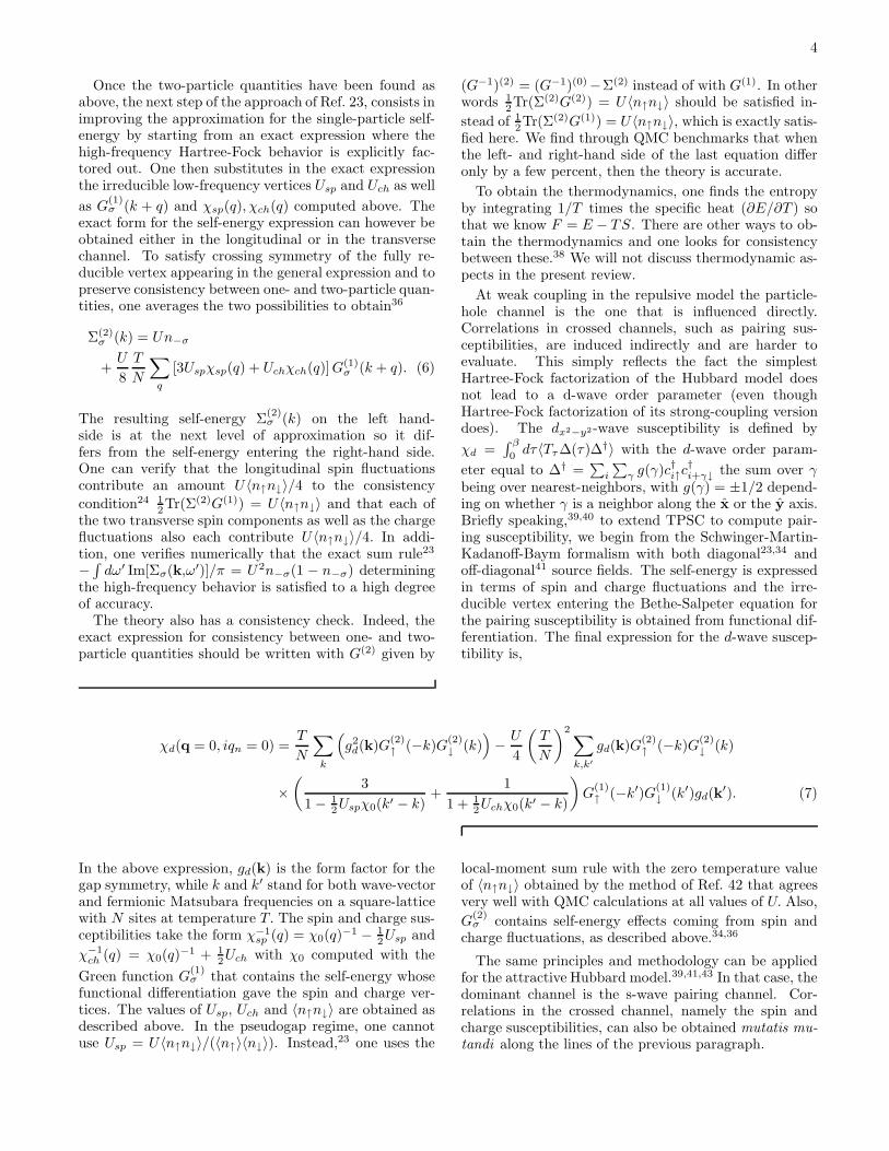
FIG. 21: MDC from CPT in the t-t′ = −0.3t, t′′ = 0.2tHubbard model, taken from Ref. 77.

Each curve is for a different wave vector (on a trajectoryshown in the inset) and is plotted as a function of fre-quency in units of t. This kind of plot is known as En-ergy Dispersion Curves (EDC). It is important to pointout that the theoretical results are obtained by broaden-ing a set of delta function, so that the energy resolutionis η = 0.12t corresponding roughly to the experimentalresolution we will compare with in the next section. Atsmall U = 2t on the top panel of Fig. 19, one recovers aFermi liquid. At large U , say U = 8t, the Mott gap atpositive energy is a prominent feature. The pseudogapis a different feature located around the Fermi energy.To see it better, we present on the left-hand panel ofFig. 20 a blow-up in the vicinity of the Fermi surfacecrossing occurring near (π, 0). Clearly, there is a mini-mum in A(k, ω) at the Fermi-surface crossing when U islarge enough instead of a maximum like in Fermi liquidtheory.

It is also possible to plot A(k, ω) at fixed frequency forvarious momenta. They are so-called Momentum Dis-persion Curves (MDC). In Fig. 21 we take the Fermienergy ω = 0, and we plot the magnitude of the single-particle spectral weight in the first quadrant of the Bril-louin zone using red for high-intensity and blue for lowintensity. The figure shows that, in the hole-doped case(top panel), weight near (π/2, π/2) survives while it tendsto disappear near (π, 0) and (0, π). That pseudogap phe-nomenon is due not only to large U but also to the factthat the line that can be drawn between the points (π, 0)and (0, π) crosses the Fermi surface. When there is nosuch crossing, one recovers a Fermi surface (not shownhere). The (π, 0) to (0, π) line has a double role. It is theantiferromagnetic zone boundary, as well as the line thatindicates where umklapp processes become possible, i.e.,the line where we can scatter a pair of particles on oneside of the Fermi surface to the other side with loss or

14

FIG. 22: Right: The corresponding EDC in the t-t′-t′′ Hub-bard model, calculated on a 16-site cluster in CPT, at n =9/8. Inset: the pseudogap. Left: The corresponding Fermienergy momentum distribution curve.

FIG. 23: EDC in the t-t′-t′′ Hubbard model, with t′ = −0.3tand t′′ = 0.2t, calculated on a 8-site cluster for U = 8tin VCPT. d-wave superconductivity is present in the holde-doped case (left) and both antiferromagnetism and d-wavesuperconductivity in the electron-doped case. The resolutionis not large enough in the latter case to see the superconduct-ing gap. The Lorentzian broadening is 0.2t. From Ref. 19.

gain of a reciprocal lattice vector. Large scattering ratesexplain the disappearance of the Fermi surface.77 We alsonote that the size of the pseudogap in CPT, defined asthe distance between the two peaks, does not scale likeJ = 4t2/U at large coupling. It seems to be very weaklyU dependent, its size being related to t instead. Thisresult is corroborated by CDMFT.67

The EDC for the electron-doped case is shown on thebottom panels of Fig. 19 near optimal doping again. Thistime, the Mott gap appears below the Fermi surface sothat the lower Hubbard band becomes accessible to ex-periment. The EDC in Fig. 22 shows very well both theMott gap and the pseudogap. Details of that pseudogapcan be seen both in the inset of Fig. 22 or on the right-hand panel of Fig. 20. While in the hole-doped case theMDC appeared to evolve continuously as we increase U(top panel of Fig. 21), in the electron-doped case (bot-tom panel) the weight initially present near (π/2, π/2) atU = 4t disappears by the time we reach U = 8t.

In Fig. 23 we show, with the same resolution as CPT,the MDC for VCPT.19 In this case the effect of long-rangeorder is included and visible but, at this resolution, theresults are not too different from those obtained fromCPT in Fig. 21.

FIG. 24: MDC in the t-t′, U = 8t Hubbard model, calculatedon a 4-site cluster in CDMFT. Energy resolution, η = 0.1t(left and middle). Left: Hole-doped dSC (t′ = −0.3t, n =0.96), Middle: Electron-doped dSC (t′ = 0.3t, n = 0.93),Right: Same as middle with η = 0.02t. Note the particle-holetransformation in the electron-doped case. From Ref. 17.

FIG. 25: EDC in the t-t′ = 0, U = 8t Hubbard model, cal-culated on a 4-site cluster in CDMFT. Top: normal (para-magnetic) state for various densities. Bottom: same for theantiferromagnetic state. From Ref. 67.

2. CDMFT and DCA

CDMFT17 gives MDC that, at comparable resolution,η = 0.1t, are again compatible with CPT and withVCPT. The middle panel in Fig. 24 is for the electron-doped case but with a particle-hole transformation sothat t′ = +0.3t and k → k + (π, π). Since there is anon-zero d-wave order parameter in this calculation, im-proving the resolution to η = 0.02t reveals the d-wavegap, as seen in the right most figure.

It has been argued for a while in DCA that thereis a mechanism whereby short-range correlations atstrong coupling can be the source of the pseudogapphenomenon.78 To illustrate this mechanism in CDMFT,we take the case t′ = t′′ = 0 and compare in Fig. 25the EDC for U = 8t without long-range order (top pan-els) and with long-range antiferromagnetic order (bot-tom panels).67 The four bands appearing in Figs 25a and25d are in agreement with what has been shown73,79,80

with CPT, VCPT and QMC in Fig. 26. Evidently thereare additional symmetries in the antiferromagnetic case.The bands that are most affected by the long-range or-der are those that are closest to the Fermi energy, hencethey reflect spin correlations, while the bands far from

15

FIG. 26: EDC in the Hubbard model, U = 8t, t′ = 0 calcu-lated in CPT, VCPT and QMC. From Ref. 73.

the Fermi energy seem less sensitive to the presence oflong-range order. These far away bands are what is leftfrom the atomic limit where we have two dispersionlessbands. As we dope, the chemical potential moves intothe lower band closest to the Fermi energy. When thereis no long-range order (Figs 25b and 25c) the lower bandclosest to the Fermi energy moves very close to it, at thesame time as the upper band closest to the Fermi energylooses weight, part of it moving closer to the Fermi en-ergy. These two bands leave a pseudogap at the Fermienergy82,83, although we cannot exclude that increasingthe resolution would reveal a Fermi liquid at a very smallenergy scale. In the case when there is long-range anti-ferromagnetic order, (Figs 25e and 25f) the upper bandis less affected while the chemical potential moves in thelower band closest to the Fermi energy but without creat-ing a pseudogap, as if we were doping an itinerant antifer-romagnet. It seems that forcing the spin correlations toremain short range leads to the pseudogap phenomenonin this case. When a pseudogap appears, it is createdagain by very large scattering rates.67

3. TPSC (including analytical results)

In Hartree-Fock theory, double occupancy is given byn2/4 and is independent of temperature. The correctresult does depend on temperature. One can observe

FIG. 27: Double occupancy 〈n↑n↓〉, in the two-dimensionalHubbard model for n = 1, as calculated from TPSC (lineswith x) and from DCA (symbols) from Ref. 81. Taken fromRef. 84.

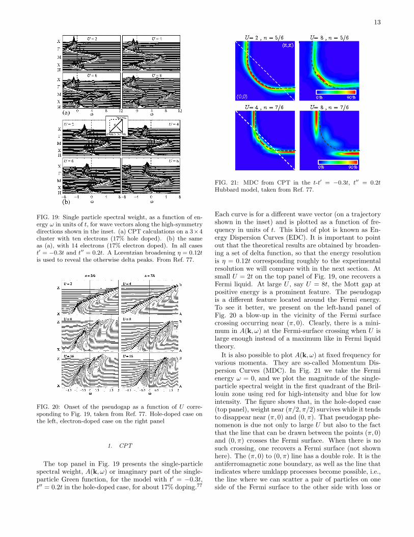
FIG. 28: MDC at the Fermi energy for the two-dimensionalHubbard model for U = 6.25, t′ = −0.175t, t′′ = 0.05t atvarious hole dopings, as obtained from TPSC. The far leftfrom Ref. 85 is the Fermi surface plot for 10% hole-dopedCa2−xNaxCuO2Cl2.

in Fig. 27 the concordance between the results for thetemperature-dependent double occupancy obtained withDCA and with TPSC84 for the t′ = t′′ = 0 model. Wehave also done extensive comparisons between straightQMC calculations and TPSC.38 The downturn at lowtemperature has been confirmed by the QMC calcula-tions. It comes from the opening of the pseudogap dueto antiferromagnetic fluctuations, as we will describe be-low. The concomitant increase in the local moment corre-sponds to the decrease in double-occupancy. There seemsto be a disagreement at low temperature between TPSCand DCA at U = 2t. In fact TPSC is closer to the di-rect QMC calculation. Since we expect quantum clustermethods in general and DCA in particular to be less ac-curate at weak coupling, this is not too worrisome. AtU = 4t the density of states obtained with TPSC andwith DCA at various temperatures are very close to eachother.84 We stress that as we go to temperatures wellbelow the pseudogap, TPSC becomes less and less ac-curate, generally overemphasizing the downfall in doubleoccupancy.

We will come back to more details on the predictionsof TPSC for the pseudogap, but to illustrate the concor-dance with quantum cluster results shown in the previ-ous subsection, we show in Fig. 28 MDC obtained at theFermi energy in the hole doped case for t′ = −0.175t,t′′ = 0.05t. Again there is quasi-particle weight near

16

FIG. 29: MDC at the Fermi energy in the electron-doped casewith t′ = −0.175t, t′′ = 0.05t and two different U ’s, U = 6.25tand U = 5.75t obtained from TPSC. The first column is thecorresponding experimental plots at 10% and 15% doping inRef. 86. From Refs. 40,87.

FIG. 30: Cartoon explanation of the pseudogap in the weak-coupling limit. Below the dashed crossover line to the renor-malized classical regime, when the antiferromagnetic corre-lation length becomes larger than the thermal de Brogliewave length, there appears precursors of the zero-temperatureBoboliubov quasiparticles for the long-range ordered antifer-romagnet.

(π/2, π/2) and a pseudogap near (π, 0) and (0, π). How-ever, as we will discuss below, the antiferromagnetic cor-relation length necessary to obtain that pseudogap is toolarge compared with experiment. The electron-dopedcase is shown in Fig. 29 near optimal doping and fordifferent values of U. As U increases, the weight near(π/2, π/2) disappears. That is in concordance with theresults of CPT shown in Fig. 21 where the weight atthat location exists only for small U. That also agreeswith slave-boson calculations88 that found such weightfor U = 6t and it agrees also with one-loop calculations89

starting from a Hartree-Fock antiferromagnetic state thatdid not find weight at that location for U = 8t. Thesimplest Hartree-Fock approach21,90 yields weight near(π/2, π/2) only for unreasonably small values of U .

A cartoon explanation of the pseudogap is given in

Fig. 30. At high temperature we have a Fermi liquid,as illustrated in panel I. Now, suppose we start from aground state with long-range order as in panel III, inother words at a filling between half-filling and nc. Inthe Hartree-Fock approximation we have a gap and thefermion creation-annihilation operators now project onBogoliubov-Valentin quasiparticles that have weight atboth positive and negative energies. In two dimensions,the Mermin-Wagner theorem means that as soon as weraise the temperature above zero, long-range order dis-appears, but the antiferromagnetic correlation length ξremains large so we obtain the situation illustrated inpanel II, as long as ξ is much larger than the thermal deBroglie wave length ξth ≡ vF /(πT ) in our usual units. Atthe crossover temperature TX then the relative size of ξand ξth changes and we recover the Fermi liquid. We nowproceed to sketch analytically where these results comefrom starting from finite temperature. Details and morecomplete formulae may be found in Refs. 23,24,33,37.Note also that a study starting from zero temperaturehas also been performed in Ref. 91.

First we show how TPSC recovers the Mermin-Wagnertheorem. Consider the self-consistency conditions givenby the local moment sum rule Eq. (4) together with theexpression for the spin-susceptibility Eq. (2) and Usp inEq. (5). First, it is clear that if the left-hand side of thelocal moment sum rule Eq. (4) wants to increase becauseof proximity to a phase transition, the right-hand side cando so only by decreasing 〈n↑n↓〉 which in turns decreasesUsp through Eq. (5) and moves the system away from thephase transition. This argument needs to be made moreprecise to include the effect of dimension. First, usingthe spectral representation one can show that every termof χsp(q, iqn) is positive. Near a phase transition, thezero Matsubara frequency component of the susceptibil-ity begins to diverge. On can check from the real-timeformalism that the zero-Matsubara frequency contribu-tion dominates when the characteristic spin fluctuationfrequency ωsp ∼ ξ−2 becomes less than temperature, theso-called renormalized-classical regime. We isolate thiscontribution on the left-hand side of the local momentsum rule and we move the contributions from the non-zero Matsubara frequencies, that are non-divergent, onthe right-hand side. Then, converting the wave vectorsum to an integral and expanding the denominator of thesusceptibility around the wave vector where the instabil-ity would occurs to obtain an Ornstein-Zernicke form,the local moment sum rule Eq. (4) can be written in theform

T

∫

qd−1dq1

q2 + ξ−2= C(T ). (28)

The constant on the right-hand side contains only non-singular contributions and ξ−2 contains Usp that we wantto find. From the above equation, one finds immediatelythat in d = 2, ξ ≈ exp(C(T )/T ) so that the correla-tion length diverges only at T = 0. In three dimensions,isotropic or not, exponents correspond to those of the

17

FIG. 31: MDC plots at the Fermi energy (upper) and corre-sponding scattering rates (lower) obtained from TPSC. Thered lines on the upper panel indicate the region where thescattering rate in the corresponding lower panels is large.

N = ∞ universality class.46

To see how the pseudogap opens up in the single-particle spectral weight, consider the expression (6) forthe self-energy. Normally one has to do the sum overbosonic Matsubara frequencies first, but the zero Mat-subara frequency contribution has the correct asymp-totic behavior in fermionic frequencies ikn so that onecan once more isolate on the right-hand side the zeroMatsubara frequency contribution. This is confirmed bythe real-time formalism23 (See also Eq. (36) below). Inthe renormalized classical regime then, we have

Σ(kF , ikn) ∝ T

∫

qd−1dq1

q2 + ξ−2

1

ikn − εkF +Q+q

(29)

where Q is the wave vector of the instability. Hence,when εkF +Q = 0, in other words at hot spots, we find af-ter analytical continuation and dimensional analysis that

ImΣR(kF , 0) ∝ −πT

∫

dd−1q⊥dq||1

q2⊥ + q2

|| + ξ−2δ(v′F q||)

(30)

∝πT

v′Fξ3−d. (31)

Clearly, in d = 4, ImΣR(kF , 0) vanishes as temperaturedecreases, d = 3 is the marginal dimension and in d = 2we have that ImΣR(kF , 0) ∝ ξ/ξth that diverges at zerotemperature. In a Fermi liquid that quantity vanishes atzero temperature. A diverging ImΣR(kF , 0) correspondsto a vanishingly small A(kF , ω = 0) as we can see from

A(k, ω) =−2 ImΣR(kF , ω)

(ω − εk − Re ΣR(kF , ω))2 + ImΣR(kF , ω)2.

(32)To see graphically this relationship between the loca-tion of the pseudogap and large scattering rates at the

Fermi surface, we draw in Fig. 31 both the Fermi surfaceMDC and, in the lower panels, the corresponding plotsfor ImΣR(k, 0). Note that at stronger U the scatteringrate is large over a broader region, leading to a depletionof A(k,ω) over a broader range of k values.

An argument for the splitting in two peaks seen inFigs. 6 and 30 is as follows. Consider the singular renor-malized contribution coming from the spin fluctuations inEq. (29) at frequencies ω ≫ vF ξ−1. Taking into accountthat contributions to the integral come mostly from aregion q ≤ ξ−1, this expression leads to

Re ΣR(kF , ω) =

(

T

∫

qd−1dq1

q2 + ξ−2

)

1

ikn − εkF +Q

≡∆2

ω − εkF +Q

(33)

which, when substituted in the expression for the spectralweight (32) leads to large contributions when

ω − εk −∆2

ω − εkF +Q

= 0 (34)

or, equivalently,

ω =(εk + εkF +Q) ±

√

(εk − εkF +Q)2 + 4∆2

2, (35)

which corresponds to the position of the hot spots inFig. 29 for example.

Note that analogous arguments hold for any fluctu-ation that becomes soft,23 including superconductingones.41,43 The wave vector Q would be different in eachcase.

4. Weak- and strong-coupling pseudogaps

The CPT results of Figs. 19 and 22 clearly show thatthe pseudogap is different from the Mott gap. At finitedoping, the Mott gap remains a local phenomenon, inthe sense that there is a region in frequency space that isnot tied to ω = 0 where for all wave vectors there are nostates. The peudogap by contrast is tied to ω = 0 andoccurs in regions nearly connected by (π, π), whether weare talking about hole- or about electron-doped cuprates.That the phenomenon is caused by short-range correla-tions can be seen in CPT from the fact that the pseu-dogap is independent of cluster shape and size (most ofthe results were presented for 3 × 4 clusters and we didnot go below size 2 × 2). The antiferromagnetic cor-relations and any other two-particle correlations do notextend beyond the size of the lattice in CPT. Hence, thepseudogap phenomenon cannot be caused by antiferro-magnetic long-range order since no such order exists inCPT. This is also vividly illustrated by the CDMFT re-sults in Fig. 25 that contrast the case with and withoutantiferromagnetic long-range order. The CDMFT resultsalso suggest that the pseudogap appears in the bands

18

that are most affected by antiferromagnetic correlationshence it seems natural to associate it with short-rangespin correlations. The value of t′ has an effect, but itmostly through the fact that it has a strong influence onthe relative location of the antiferromagnetic zone bound-ary and the Fermi surface, a crucial factor determiningwhere the pseudogap is. All of this as well as many re-sults obtained earlier by DCA78 suggest that there is astrong coupling mechanism that leads to a pseudogap inthe presence of only short-range two-body correlations.However, the range cannot be zero. Only the Mott gapappears at zero range, thus the pseudogap is absent insingle-site DMFT.

In the presence of a pseudogap at strong coupling(U > 8t), wave vector is not, so to speak, such a badquantum number in certain directions. In other wordsthe wave description is better in those directions. Inother directions that are “pseudogapped”, it is as if thelocalized, or particle description was better. This com-petition between wave and particle behavior is inherentto the Hubbard model. At the Fermi surface in low di-mension, it seems that this competition is resolved bydividing (it is a crossover, not a real division) the Fermisurface in different sections.

There is also a weak-coupling mechanism for the pseu-dogap. This has been discussed at length just in the pre-vious section on TPSC. Another way to rephrase the cal-culations of the previous section is in the real frequencyformalism. There one finds23 that

Σ′′R(kF , ω)

∝

∫

dd−1q⊥(2π)d−1

∫

dω′

π[n(ω′) + f(ω + ω′)]χ′′

sp(q; ω′)

(36)

so that if the characteristic spin fluctuation frequencyin χ′′

sp(q; ω′) is much larger than temperature, then[n(ω′)+f(ω+ω′)] can be considered to act like a windowof size ω or T and χ′′

sp(q; ω′) can be replaced by a func-tion of q times ω′ which immediately leads to the Fermiliquid result [ω2 +(πT )2]. In the opposite limit where thecharacteristic spin fluctuation frequency in χ′′

sp(q; ω′) ismuch less than temperature, then it acts as a windownarrower than temperature and [n(ω′) + f(ω + ω′)] canbe approximated by the low frequency limit of the Bosefactor, namely T/ω′. Using the thermodynamic sum rule,that immediately leads to the result discussed before inEq.(31), ImΣ(kF , 0) ∝ (πT/v′F )ξ3−d. This mechanismfor the pseudogap needs long correlation lengths. InCPT, this manifests itself by the fact that the apparentpseudogap in Fig. 21 at U = 4t is in fact mostly a depres-sion in spectral weight that depends on system size andshape. In addition, in contrast to the short-range strong-coupling mechanism, at weak coupling the pseudogap ismore closely associated with the intersection of the anti-ferromagnetic zone boundary with the Fermi surface.

Which mechanism is important for the cuprates willbe discussed below in the section on comparisons withexperiments.

B. d-wave superconductivity

The existence of d-wave superconductivity at weakcoupling in the Hubbard model mediated by theexchange of antiferromagnetic fluctuations92,93 hadbeen proposed even before the discovery of high-temperature superconductivity.6–8 At strong-coupling,early papers13,14 also proposed that the superconductiv-ity would be d-wave. The issue became extremely contro-versial, and even recently papers have been published12

that suggest that there is no d-wave superconductivityin the Hubbard model. That problem could have beensolved very long ago through QMC calculations if it hadbeen possible to do them at low enough temperature.Unfortunately, the sign problem hindered these simula-tions, and the high temperature results5,44,95,96 were notencouraging: the d-wave susceptibility was smaller thanfor the non-interacting case. Since that time, numericalresults from variational QMC,4,97 exact diagonalization16

and other numerical approaches98 for example, suggestthat there is indeed d-wave superconductivity in the Hub-bard model.

In the first subsection, we show that VCPT leads toa zero-temperature phase diagram for both hole andelectron-doped systems that does show the basic featuresof the cuprate phase diagram, namely an antiferromag-netic phase and a d-wave superconducting phase in dop-ing ranges that are quite close to experiment19 (The fol-lowing section will treat in more detail comparisons withexperiment). The results are consistent with CDMFT.17

The fall in the d-wave superconducting order parameternear half-filling is associated with the Mott phenomenon.The next subsection stresses the instability towards d-wave superconductivity as seen from the normal stateand mostly at weak coupling. We show that TPSC canreproduce available QMC results and that its extrapo-lation to lower temperature shows d-wave superconduc-tivity in the Hubbard model. The transition tempera-ture found at optimal doping40 for U = 4t agrees withthat found by DCA,18 a result that could be fortuitous.But again the concordance between theoretical resultsobtained at intermediate coupling with methods that arebest at opposite ends of the range of coupling strengthsis encouraging.

1. Zero-temperature phase diagram

In VCPT, one adds to the cluster Hamiltonian theterms19

H ′M = M

∑

µ

eiQ·Rµ(nµ↑ − nµ↓) (37)

H ′D = D

∑

µν

gµν(cµ↑cν↓ + H.c.) (38)

with M and D are respectively antiferromagnetic and d-wave superconducting Weiss fields that are determined

19

FIG. 32: Antiferromagnetic (bottom) and d-wave (top) orderparameters for U = 8t, t′ = −0.3t t′′ = 0.2t as a function ofthe electron density (n) for 2 × 3, 2 × 4 and 10-site clusters,calculated in VCPT. Vertical lines indicate the first dopingwhere only d-wave order is non-vanishing. From Ref. 19.

FIG. 33: d-wave order parameter as a function of n for variousvalues of t′, calculated in CDMFT on a 2× 2 cluster for U =8t. The positive t′ case corresponds to the electron-dopedcase when a particle-hole transformation is performed. FromRef. 17.

self-consistently and gµν equal to ±1 on near-neighborsites following the d-wave pattern. We recall that thecluster Hamiltonian should be understood in a varia-tional sense. Fig. 32 summarizes, for various cluster sizes,the results for the d-wave order parameter D0 and for theantiferromagnetic order parameter M0 for a fixed value ofU = 8t and the usual hopping parameters t′ = −0.3t andt′′ = 0.2t. The results for antiferromagnetism are quiterobust and extend over ranges of dopings that correspondquite closely to those observed experimentally. Despitethe fact that the results for d-wave superconductivity stillshow some size dependence, it is clear that supercon-ductivity alone without coexistence extends over a muchbroader range of dopings on the hole-doped than on theelectron-doped side as observed experimentally. VCPTcalculations on smaller system sizes99 but that include,for thermodynamic consistency, the cluster chemical po-tential as a variational parameter show superconductivity

FIG. 34: Antiferromagnetic (bottom) and d-wave (top) orderparameters as a function of the electron density (n) for t′ =−0.3t t′′ = 0.2t and various values of U on a 8-site cluster,calculated in VCPT. From Ref. 19.

FIG. 35: d-wave order parameter as a function of n for variousvalues of U , and t′ = t′′ = 0 calculated in CDMFT on a 4-sitecluster. From Ref. 17.

that extends over a much broader range of dopings. Also,for small 2×2 clusters, VCPT has stronger order parame-ter on the electron than on the hole-doped side, contraryto the results for the largest system sizes in Fig. 32. Thisis also what is found in CDMFT as can be seen in Fig. 33.It is quite likely that the zero-temperature Cooper pairsize is larger than two sites, so we consider the results for2 × 2 systems only for their qualitative value.

Concerning the question of coexistence with antifer-romagnetism, one can see that it is quite robust on theelectron-doped side whereas on the hole-doped side, itis size dependent. That suggests that one should alsolook at inhomogeneous solutions on the hole-doped sidesince stripes are generally found experimentally near theregions where antiferromagnetism and superconductivitymeet.

Fig. 34 shows clearly that at strong coupling the sizeof the order parameter seems to scale with J , in otherwords it decreases with increasing U. This is also foundin CDMFT,17 as shown in Fig. 35 for t′ = t′′ = 0.

If we keep the antiferromagnetic order parameter tozero, one can check with both VCPT and CDMFT(Fig. 33) that the d-wave superconducting order parame-

20

FIG. 36: VCPT calculations for U = 4t, t′ = t′′ = 0 nearhalf-filling on 2 × 4 lattice. Contrary to the strong couplingcase, the d-wave order parameter D0 survives all the way tohalf-filling at weak coupling, unless we also allow for antifer-romagnetism.

ter goes to zero at half-filling. This is clearly due to Mottlocalization. Indeed, at smaller U = 4t for example, theorder parameter does not vanish at half-filling if we donot allow for long-range antiferromagnetic order, as il-lustrated in Fig. 35 for CDMFT.17 The same result wasfound in VCPT, as shown in Fig.36.19 Restoring long-range antiferromagnetic order does however make the d-wave order parameter vanish at half-filling.

There are thus two ways to make d-wave superconduc-tivity disappear at half-filling, either through long anti-ferromagnetic correlation lengths94 or through the Mottphenomenon. In the real systems, that are Mott insula-tors and also antiferromagnets at half-filling, both effectscan contribute.

2. Instability of the normal phase

In the introduction to this section, we alluded to QMCcalculations for the d-wave susceptibility.5,44,95,96 Recentresults40 for that quantity as a function of doping for var-ious temperatures and for U = 4t, t′ = t′′ = 0 are shownby symbols in Fig. 8. For lower temperatures, the signproblem prevents the calculation near half-filling. Yet,the lowest temperature is low enough that a dome shapebegins to appear. Nevertheless, comparison with the non-interacting case, shown by the top continuous line, leadsone to believe that interactions only suppress d-wave su-perconductivity. We can easily understand why this isso. As we already know, the TPSC results obtained fromEq. (7) are very close to the QMC calculations, as shownby the solid lines in Fig. 8. In the temperature rangeof interest, the main contribution comes from the firstterm in Eq. (7). That term represents the contributionto the susceptibility that comes from dressed quasiparti-cles that do not interact with each other. Since dressedquasiparticles have a lifetime, a pair breaking effect, it isnormal that this contribution to the interacting suscep-

FIG. 37: Tc as a function of doping, δ = 1 − n, for t′ = t′′ =0 calculated in TPSC using the Thouless criterion. FromRef. 40.

tibility leads to a smaller contribution than in the non-interacting case. At the lowest temperature, β = 4/t,the vertex contribution represented by the second termin Eq. (7) accounts for about 20% of the total. It goesin the direction of increasing the susceptibility. As wedecrease the temperature further in TPSC, that term be-comes comparable with the first one. Since the vertex inEq. (7) accounts for the exchange of a single spin wave,equality with the first term signals the divergence of theseries, as in 1/(1 − x) ∼ 1 + x. The divergence of thatseries represents physically the instability of the normalphase to a d-wave superconducting phase. This is analo-gous to the Thouless criterion and hence it gives an up-per bound to Tc. In other words, Berezinskii-Kosterlitz-Thouless physics is not included.

Fig. 37 shows the TPSC transition temperature forU = 4t and for U = 6t. As we move towards half-filling, located to the left of the diagram, starting fromlarge dopings, Tc goes up because of the increase in anti-ferromagnetic fluctuations. Eventually, Tc turns aroundand decreases because of the opening of the pseudogap.Physically, when the pseudogap opens up, weight is re-moved from the Fermi level, the density of states be-comes very small, and pairing cannot occur any more.In the FLEX approximation22,100 that does not exhibit apseudogap,101 that downturn, observed already in QMCat high temperature, does not occur. We have observedthat in cases where t′ 6= 0 so that the pseudogap opensonly in a limited region around hot spots, the downturncan become less pronounced.

The case n = 0.9 = 1 − δ that corresponds to opti-mal doping for U = 4t in Fig. 37 has been studied byDCA. In an extensive and systematic study of the sizedependence, Maier et al.18 established the existence ofa d-wave instability at a temperature that coincides towithin a few percent with the result in Fig. 37. Since veryfew vortices can fit within even the largest cluster sizesstudied in Ref. 18, it is quite likely that the Tc that theyfind does not include Berezinskii-Kosterlitz-Thouless ef-fects, just like ours. Despite the fact that, again, the

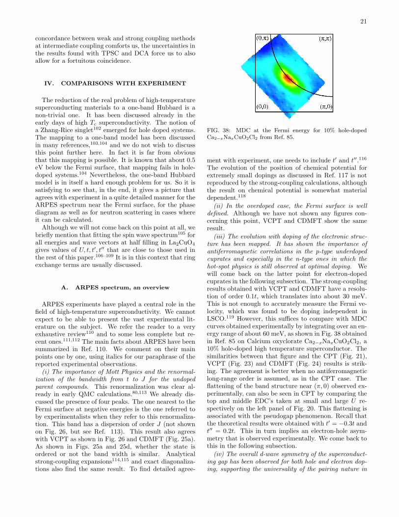
21

concordance between weak and strong coupling methodsat intermediate coupling comforts us, the uncertainties inthe results found with TPSC and DCA force us to alsoallow for a fortuitous coincidence.

IV. COMPARISONS WITH EXPERIMENT

The reduction of the real problem of high-temperaturesuperconducting materials to a one-band Hubbard is anon-trivial one. It has been discussed already in theearly days of high Tc superconductivity. The notion ofa Zhang-Rice singlet102 emerged for hole doped systems.The mapping to a one-band model has been discussedin many references,103,104 and we do not wish to discussthis point further here. In fact it is far from obviousthat this mapping is possible. It is known that about 0.5eV below the Fermi surface, that mapping fails in hole-doped systems.104 Nevertheless, the one-band Hubbardmodel is in itself a hard enough problem for us. So it issatisfying to see that, in the end, it gives a picture thatagrees with experiment in a quite detailed manner for theARPES spectrum near the Fermi surface, for the phasediagram as well as for neutron scattering in cases whereit can be calculated.

Although we will not come back on this point at all, webriefly mention that fitting the spin wave spectrum105 forall energies and wave vectors at half filling in La2CuO4

gives values of U, t, t′, t′′ that are close to those used inthe rest of this paper.106–109 It is in this context that ringexchange terms are usually discussed.

A. ARPES spectrum, an overview

ARPES experiments have played a central role in thefield of high-temperature superconductivity. We cannotexpect to be able to present the vast experimental lit-erature on the subject. We refer the reader to a veryexhaustive review110 and to some less complete but re-cent ones.111,112 The main facts about ARPES have beensummarized in Ref. 110. We comment on their mainpoints one by one, using italics for our paraphrase of thereported experimental observations.

(i) The importance of Mott Physics and the renormal-ization of the bandwidth from t to J for the undopedparent compounds. This renormalization was clear al-ready in early QMC calculations.80,113 We already dis-cussed the presence of four peaks. The one nearest to theFermi surface at negative energies is the one referred toby experimentalists when they refer to this renormaliza-tion. This band has a dispersion of order J (not shownon Fig. 26, but see Ref. 113). This result also agreeswith VCPT as shown in Fig. 26 and CDMFT (Fig. 25a).As shown in Figs. 25a and 25d, whether the state isordered or not the band width is similar. Analyticalstrong-coupling expansions114,115 and exact diagonaliza-tions also find the same result. To find detailed agree-

FIG. 38: MDC at the Fermi energy for 10% hole-dopedCa2−xNaxCuO2Cl2 from Ref. 85.

ment with experiment, one needs to include t′ and t′′.116

The evolution of the position of chemical potential forextremely small dopings as discussed in Ref. 117 is notreproduced by the strong-coupling calculations, althoughthe result on chemical potential is somewhat materialdependent.118

(ii) In the overdoped case, the Fermi surface is welldefined. Although we have not shown any figures con-cerning this point, VCPT and CDMFT show the sameresult.

(iii) The evolution with doping of the electronic struc-ture has been mapped. It has shown the importance ofantiferromagnetic correlations in the p-type underdopedcuprates and especially in the n-type ones in which thehot-spot physics is still observed at optimal doping. Wewill come back on the latter point for electron-dopedcuprates in the following subsection. The strong-couplingresults obtained with VCPT and CDMFT have a resolu-tion of order 0.1t, which translates into about 30 meV.This is not enough to accurately measure the Fermi ve-locity, which was found to be doping independent inLSCO.119 However, this suffices to compare with MDCcurves obtained experimentally by integrating over an en-ergy range of about 60 meV, as shown in Fig. 38 obtainedin Ref. 85 on Calcium oxyclorate Ca2−xNaxCuO2Cl2, a10% hole-doped high temperature superconductor. Thesimilarities between that figure and the CPT (Fig. 21),VCPT (Fig. 23) and CDMFT (Fig. 24) results is strik-ing. The agreement is better when no antiferromagneticlong-range order is assumed, as in the CPT case. Theflattening of the band structure near (π, 0) observed ex-perimentally, can also be seen in CPT by comparing thetop and middle EDC’s taken at small and large U re-spectively on the left panel of Fig. 20. This flattening isassociated with the pseudogap phenomenon. Recall thatthe theoretical results were obtained with t′ = −0.3t andt′′ = 0.2t. This in turn implies an electron-hole asym-metry that is observed experimentally. We come back tothis in the following subsection.

(iv) The overall d-wave symmetry of the superconduct-ing gap has been observed for both hole and electron dop-ing, supporting the universality of the pairing nature in

22

the cuprates. In the next to next subsection, we discussthe phase diagram for competing antiferromagnetism andd-wave superconductivity and show striking similaritieswith the observations.

(v) A normal-state pseudogap has been observed toopen up at a temperature T ∗ > Tc in the underdopedregime with a d-wave form similar to the one of the su-perconducting gap. That statement is correct only in thehole-doped compounds. In electron-doped systems thepseudogap has a form that is not of d-wave shape. IfTc comes from a universal pairing mechanism, a univer-sal mechanism may also be behind the pseudogap. Aswe have already discussed however, there are quantita-tive differences between strong and weak coupling mecha-nisms for both Tc and the pseudogap. For electron-dopedsystems, we made quantitative predictions for the valueof T ∗ that have later been confirmed experimentally. Allthis is discussed further below. To date, in cluster meth-ods the pseudogap temperature has been studied onlywith DCA.78

(vi) A coherent quasiparticle peak below Tc has beenobserved near (π, 0) whose spectral weight scales with thedoping level x in the underdoped regime. We expectthat it is a general result that long-range order will re-store quasiparticle like excitations in strongly correlatedsystems because gaps remove scattering channels nearthe Fermi level. This is clearly illustrated by comparingthe upper and lower panels in Fig. 25 that contrast thesame spectra with and without antiferromagnetic long-range order. We have not performed the analysis of ourresults yet that could tell us whether the spectral weightof the quasiparticle scales with x in the hole-underdopedregime. Our resolution may not be good enough to seethe quasiparticle peak. Sharpening of the quasiparti-cle excitations in the superconducting state has howeverbeen observed in DCA.120

(vii) The presence of an energy scale of about 40 −80 meV in the quasiparticle dynamics manifests itselfthrough a sharp dispersion renormalization and drop inthe scattering rate observed at those energies at differ-ent momenta. In hole-doped systems there is a kink inthe nodal direction that is already seen above Tc whilein the antinodal direction it appears only below Tc. Theenergy scales and doping dependences of these two kinksare also different.121 The energy resolution in VCPT andCDMFT is not sufficient to distinguish these subtleties.In electron-doped cuprates experiments122 suggest thatthere is no observable kink feature, in agreement withthe results presented in the following subsection.

B. The pseudogap in electron-doped cuprates

The ARPES spectrum of electron-doped cuprates isstrikingly different from that of their hole-doped coun-terpart. The Fermi energy MDC’s for the first quadrantof the Brillouin zone86 are shown at the top of Fig. 39 forthree different dopings. There is a very clear evolution

FIG. 39: Doping dependence of the MDC from experimentson NCCO with the corresponding EDC. From Ref. 86

with doping. At the lowest dopings, there is no weightnear (π/2, π/2), contrary to the hole-doped case shownin Fig. 38. For all dopings there is weight near (π, 0) in-stead of the pseudogap that appeared there in the hole-doped case. The EDC’s, also shown on the bottom ofFig. 39, are drawn for a trajectory in the Brillouin zonethat follows what would be the Fermi surface in the non-interacting case. Regions that are more green than redon the corresponding MDC’s along that trajectory are re-ferred to as hot spots. On the EDC’s we clearly see thathot spots do not correspond to simply a decrease in thequasiparticle weight Z. They truly originate from a pseu-dogap, in other words from the fact that the maximumis pushed away from zero energy. Even though the mea-surements are done at low temperature (T = 10 − 20K)the energy resolution of about 60 meV makes the su-perconducting gap invisible. What is observed at thisresolution is the pseudogap.

The contrast between the location of the pseudogap inthe hole and electron-doped compounds is clearly seenin Fig. 40 obtained from VCPT.19 In that figure, themagnitude of the spectral weight is represented by thedifferent colors as a function of frequency (in units of t)along different cuts of the Brillouin zone. In the bottompanel, for the hole-doped case, one observes the pseudo-gap near (π, 0). In the top panel, for the electron-dopedcase, it is only by zooming (inset) on the region for theFermi energy crossing near (π, 0) that one sees the d-wave superconducting gap. At 10% electron-doping, thepseudogap near (π/2, π/2) is apparent. In this case thereis antiferromagnetic long-range order, but even if we useCPT that does not exhibit long-range order, there ap-pears a pseudogap in that region.160 The main differ-ence between CPT and VCPT results is the bending backof the bands (for example around the symmetry axis at(π/2, π/2)) caused by halving of the size of the Brillouin

23

FIG. 40: Intensity plot of the spectral function as a functionof ω in units of t and wave vector from VCPT for U = 8tt′ = −0.3t, t′′ = 0.2t and n = 0.93 at the bottom and n = 1.10(electron-doped) at the top. The Lorentzian broadening is0.12t in the main figure and 0.04t in the inset that displaysthe d-wave gap. Top panel is for the electron-doped case inthe right-hand panel of Fig. 23, while bottom panel is for thehole-doped case on the left of Fig. 23. From Ref. 19.

FIG. 41: Experimental Fermi surface plot (MDC at the Fermienergy) for NCCO (left) and corresponding energy distribu-tion curves (right) for 15% electron-doping. From Ref. 86

zone in the antiferromagnetic case. Form factors90 aresuch that the intensity is not symmetric even if the dis-persion is. The faint band located at an energy about tbelow the Fermi energy near (π/2, π/2) was also found inRef. 89 by a one-loop spin-wave calculation around theHartree-Fock antiferromagnetic ground state at U = 8t.Experimentalists86 have suggested the existence of thesestates. The VCPT results go well beyond the spin-wave

FIG. 42: EDC A<(k, ω) ≡ A(k, ω)f(ω) along the Fermi sur-face calculated in TPSC (left) at optimal doping for t′ =−0.175t, t′′ = 0.05t, t = 350 meV and corresponding ARPESdata on NCCO (right). From Ref. 87.

FIG. 43: EDC A<(k, ω) ≡ A(k, ω)f(ω) along two other di-rections calculated for t′ = −0.175t, t′′ = 0.05t, t = 350 meVin TPSC (left column) and corresponding ARPES data onNCCO (right column). From Ref. 87.

calculation (dashed lines in Fig. 40) since one can alsosee numerous features in addition to remnants of the lo-calized atomic levels around +5t and −10t.

The optimally doped case is the real challenge forstrong-coupling calculations. The spin-wave approach inRef. 89 never shows the weight near (π/2, π/2) that isseen in experiment (Fig. 41). Early mean-field calcula-tions by Kusko et al.90 suggest that this (π/2, π/2) fea-ture appears for U = 3t. This is very small comparedwith U of the order of the bandwidth 8t necessary tohave a Mott insulator at half-filling. We already dis-cussed in Sec. III A that both CPT and TPSC showthat weight near (π/2, π/2) appears for U not too large,say of order 6t. This same result is also obtained in theKotliar-Ruckenstein slave boson approach.88

Since TPSC is valid for a system of infinite size,we present detailed comparisons87 with experiment86

on Nd1.85Ce0.15CuO4, an electron-doped cuprate. Wetake t′ = −0.175t, t′′ = 0.05t. Results obtained witht′ = −0.275 are very close to those we present. With thevalues used in CPT, t′ = −0.3t, t′ = 0.2t, U = 6t, TPSC

24

FIG. 44: EDC A<(k, ω) ≡ A(k, ω)f(ω) along the Fermi sur-face shown in the insets for (b) n = 1.10, U = 6.25t. Linesare shifted by a constant for clarity. From Ref. 87.

does not lead to strong enough antiferromagnetic fluc-tuations to obtain non-trivial effects in the temperaturerange studied, β = 20t. We take t = 350 meV. Fig. 39shows the correspondence between EDC and MDC. Com-parisons with experimental EDC at wave vectors alongthe non-interacting Fermi surface appear in Fig. 42 forU = 5.75t and 15% doping (n = 1.15). The dashed linesindicate the quite detailed agreement between theory andexperiment. At the hot spot, (middle dashed line), theweight is pushed back about 0.2 eV and there is a verysmall peak left at the Fermi surface, as in the experiment.If U is not large enough the antiferromagnetic fluctua-tions are not strong enough to lead to a pseudogap. As inCPT (Fig. 21), if U is too large the (π/2, π/2) weight dis-appears, as illustrated earlier in Fig. 29. In Fig. 43, cutsalong the (0, 0) to (π, π) and (0.65π, 0) to (0.65π, π) di-rections are compared with experiment. Again the peakpositions and widths are very close, except for some ex-perimental tails extending in the large binding energydirection. The theoretical results have similar asymme-try, but not as pronounced. Experimentally, the largebinding energy tails (“the background”) are the leastreproducible features from sample to sample, especiallyfor wave vectors near the Fermi surface”.161 The experi-mental renormalized Fermi velocities are 3.31 × 105 m/sand 3.09 × 105 m/s along the zone diagonal and alongthe (π, 0)-(π, π) direction, respectively. The correspond-ing renormalized Fermi velocities obtained by TPSC are3.27 × 105 m/s and 2.49 × 105 m/s, respectively. Theagreement is very good, particularly along the diagonaldirection. The bare Fermi velocities are renormalized inTPSC by roughly a factor of two.123

As we move towards half-filling, we have to increase Uslightly to find agreement with experiment, as discussedearlier in Fig. 29. Fig. 44 shows how well the EDC’s agreefor a Fermi surface cut at 10% doping (n = 1.10). Theincrease is expected physically from the fact that withfewer electrons the contribution to screening that comesfrom Thomas Fermi physics should not be as good. Thisis also consistent with the fact that a larger value of Uis necessary to explain the Mott insulator at half-filling.It would also be possible to mimic the ARPES spectrumby keeping U fixed and changing the hopping parameters,

FIG. 45: Hot spots from quasi-static scatterings off antiferro-magnetic fluctuations (renormalized classical regime).

FIG. 46: Semi-log plot of the AFM correlation length (in unitsof the lattice constant) against inverse temperature (in unitsof J = 125 meV). Filled symbols denote calculated resultsand empty ones experimental data of Ref. 124 and Ref. 125(x = 0.15). From Ref. 87.

but the changes would be of order 20%, which does notappear realistic.87

We have already explained that the physics behind thepseudogap in TPSC is scattering by nearly critical anti-ferromagnetic fluctuations. This is illustrated in Fig. 45.If this explanation is correct, the antiferromagnetic cor-relation length measured by neutron scattering shouldbe quite large. The results of the measurement124,125

and of the TPSC calculations are shown in Fig. 46. Theagreement is again surprisingly good. As we move tosmaller dopings n = 1.1 (not shown) the agreement be-comes less good, but we do expect TPSC to deteriorateas U increases with underdoping. The arrow points tothe temperature where EDC’s shown earlier were calcu-lated. Note however that the neutron measurements weredone on samples that were not reduced, by contrast withthe ARPES measurements mentioned earlier. We are ex-pecting experiments on this subject.162. We should pointout that the EDC’s depend strongly on temperature andon the actual value of the antiferromagnetic correlationlength only in the vicinity of the temperature where thereis a crossover to the pseudogap regime. Decreasing the

25

FIG. 47: Pseudogap temperature T ∗ (filled circles de-note T ∗ calculated from TPSC, empty ones experimentaldata extracted from optical conductivity.127) Empty trian-gles are experimental Neel temperatures TN . The samplesare reduced.124 From Ref. 87.

temperature makes the ω = 0 peaks near (π, 0) sharper87

as observed experimentally.126

The ARPES pseudogap temperature T ∗ has been pre-dicted with TPSC.87 The predictions are shown by thesolid line in Fig. 47. The pseudogap temperature ob-served in optical experiments127 is shown by the opencircles. It differs from the ARPES result, especially aswe move towards optimal doping. The size of the pseu-dogap observed in the optical experiments127 (10T ∗) iscomparable to the ARPES pseudogap. The solid line inFig. 47 contains several predictions. If we look at 13%doping (n = 1.13), the line predicts T ∗ ∼ 250K. Ex-periments that were done without being aware of thisprediction128 have verified it. It would be most inter-esting to do neutron scattering experiments on the samesamples to check whether the antiferromagnetic corre-lation length ξ and the thermal de Broglie wave lengthξth are comparable at that temperature, as predicted byTPSC. Fig. 47 also predicts that the pseudogap inducedby antiferromagnetic fluctuations will disappear at thequantum critical point where long-range antiferromag-netic order disappears, in other words it will coincidewith the crossing of the experimentally observed Neeltemperature (dashed line with triangles in Fig. 47) withthe zero temperature axis (if that crossing is not maskedby the superconducting transition). Recent optical con-ductivity experiments129,130 confirm this prediction aswell.

In TPSC, superconducting fluctuations can also leadto a pseudogap by an analogous mechanism.23

C. The phase diagram for high-temperature

superconductors

The main features appearing in the phase diagramof high-temperature superconductors are the pseudogapphase, the antiferromagnetic phase and the d-wave su-perconducting phase. Fig. 48110 shows the typical dia-gram with hole doping to the right and electron dopingto the left. Zero on the horizontal axis corresponds to

FIG. 48: The generic phase diagram of high-Tc superconduc-tors, from Ref. 110. There should also be a pseudogap line onthe electron-doped side. It was not well studied at the timeof publication of that paper.

FIG. 49: Antiferromagnetic order parameter m (dashed) andd-wave (solid) order parameter obtained from CDMFT on a2 × 2 cluster. The result obtained by forcing m = 0 is alsoshown as a thin dashed line.

half-filling. There are other features on the phase di-agram, in particular checkerboard patterns131 or stripephases132 that appear in general close to the region whereantiferromagnetism and superconductivity come close toeach other. Before we try to understand these more de-tailed features, one should understand the most impor-tant phases. In the previous subsection we have discussedthe pseudogap phase, in particular on the electron-dopedside (not indicated on Fig. 48). A recent review of thepseudogap appears in Ref. 133. In the following, we dis-cuss in turn the phase diagram and then the nature ofthe superconducting phase itself and its relation to theMott phenomenon.

1. Competition between antiferromagnetism andsuperconductivity

We have already shown in Fig. 32 the prediction ofVCPT for the zero-temperature phase diagram.19 Here,we just point out how closely the position of the anti-ferromagnetic phase boundary, appearing in the lowerpanel, coincides with the experimental phase diagram in

26

Fig. 48. (Note that electron concentration increases fromright to left on this experimental phase diagram). In par-ticular, there is little size dependence to the position ofthis boundary, (6 to 10 sites) and in addition the depen-dence on the value of U is also weak, as can be seen fromFig. 34. Hence, the positions of the antiferromagneticphase boundaries is a robust prediction of VCPT. TheCDMFT result for a four site cluster in a bath is shownin Fig. 49 for t′ = −0.3t, t′′ = 0 and U = 8t. The agree-ment with experiment is not as good. Despite the usefulpresence of a bath in CDMFT, the cluster itself is of size2 × 2, which is probably smaller than the Cooper pairsize. We can obtain results closer to those of VCPT byincreasing the variational space.

The d-wave superconducting order parameter on thetop panel of Fig. 32 shows more size dependence thanthe antiferromagnetic order parameter. Nevertheless,there are some clear tendencies: (a) d-wave supercon-ductivity can exist by itself, without antiferromagnetism.The vertical lines indicate the location of the end ofthe antiferromagnetic phase for the various system sizesto help this observation. (b) The range where d-wave-superconductivity exists without antiferromagnetism, isabout three times larger on the hole than on the electron-doped side, as observed experimentally. (c) As systemsize increases, the maximum d-wave order parameteris larger on the hole than on the electron-doped side.(d) The tendency to have coexisting antiferromagnetismand d-wave superconductivity is rather strong on theelectron-doped side of the phase diagram. This is ob-served experimentally134 but only over a rather narrowregion near optimal doping. Recent experiments135 chal-lenge this result, others136,137 indicate that antiferromag-netism can be induced from the d-wave superconductingphases with very small fields. (e) On the hole-doped side,d-wave superconductivity and antiferromagnetism coex-ist for a very narrow range of dopings for system sizeNc = 6, for a broad range extending to half-filling forNc = 8 and not at all for Nc = 10. In other words,the tendency to coexistence is not even monotonic. Weinterpret this result as a reflection of the tendency toform stripes observed experimentally on the hole-dopedside.132,138,139 We cannot study systems large enoughto allow for striped inhomogeneous states to check thisstatement.

The more realistic two-band model has also been stud-ied using DCA.104 The results are shown on Fig. 50.Electron concentration increases from right to left. Thisphase diagram is very close to that obtained with thesame method from the one-band Hubbard model104 witht′ = −0.3t, t′′ = 0, U = 8t. The qualitative results agreewith the other calculations and with experiment: anti-ferromagnetism extends over a narrower doping range forhole than for electron doping and d-wave superconductiv-ity by itself exists over a broader range for the hole-dopedcase than for the electron-doped case. The actual rangeswhere antiferromagnetism and d-wave superconductivityexist are not in as good an agreement with experiment

FIG. 50: Phase diagram obtained from DCA for U = 8t forthe two-band model. From Ref. 104

as in the VCPT case. However, as in CDMFT, the sys-tem sizes, 2 × 2, are very small. Overall then, quantumcluster methods, VCPT in particular, allow us to obtainfrom the Hubbard model the two main phases, antifer-romagnetic and d-wave superconducting, essentially inthe observed doping range of the zero-temperature phasediagram. At finite temperature, DCA and TPSC agreeon the value of Tc for the particle-hole symmetric modelat 10% doping and U = 4t. Recent studies of the irre-ducible vertex using DCA140 also show that in the weak-coupling limit the particle-particle d-wave channel leadsto an instability driven by antiferromagnetic fluctuationsas temperature decreases, as found in TPSC.

To understand the effect of pressure on the phase dia-gram, note that U/t should decrease as pressure increasessince the increase in the overlap between orbitals shouldlead mainly to an increase in t. Hence, as can be de-duced from Fig. 37, applying pressure should lead to adecrease in the value of Tc at weak coupling, concomi-tant with the decrease in antiferromagnetic fluctuationsthat lead to pairing in the weak coupling case. This isindeed what pressure does experimentally in the case ofelectron-doped high-temperature superconductors,141 re-inforcing our argument that near optimal doping they aremore weakly coupled. It is widely known on the otherhand that pressure increases Tc in hole-doped systems.That is consistent with the strong-coupling result thatwe found in VCPT and CDMFT, namely that the max-imum d-wave order parameter in that case scales withJ = 4t2/U, a quantity that increases with t and hencepressure. Whereas in the weak coupling case supercon-ductivity is a secondary phenomenon that occurs afterantiferromagnetic fluctuations have built up, in strongcoupling they can be two distinct phenomena as can beseen from the phase diagram, even though they arise fromthe same microscopic exchange interaction representedby J .

27

2. Anomalous superconductivity near the Mott transition

Superconductivity in the underdoped regime is verymuch non-BCS. First of all, we notice in Fig. 35 ob-tained in CDMFT17 that at strong coupling the d-wavesuperconducting order parameter vanishes as we movetowards half-filling even in the absence of long-range an-tiferromagnetic order. In other words, the Mott phe-nomenon by itself suffices to destroy d-wave superconduc-tivity. This conclusion is reinforced by the fact that atweak coupling (U = 4t) where there is no Mott localiza-tion, d-wave superconductivity survives at half-filling. Inthe presence of antiferromagnetic long-range order, thatlast statement would not be true, as confirmed by VCPTcalculations in Fig. 36: at U = 4t d-wave superconduc-tivity survives at half-filling if we do not allow for an-tiferromagnetic long-range order but it disappears if wedo. In BCS theory, the presence of an interaction J thatleads to attraction in the d-wave channel would lead atT = 0 to d-wave superconductivity at all dopings includ-ing half-filling, unless we allow for competing long-rangeorder. At strong coupling, no long-range order is neces-sary to destroy d-wave superconductivity.

Superconductivity at strong coupling142,143 also differsfrom BCS in the origin of the condensation energy. Sup-pose we do BCS theory on the attractive Hubbard model.Then, as in the usual BCS model, kinetic energy is in-creased in the superconducting state because the Fermisurface is no-longer sharp. On the other hand, in thesuperconducting phase there is a gain in potential en-ergy. The reverse is true at strong coupling. This re-sult follows from DCA120 and is in agreement with thekinetic energy drop in the superconducting state thathas been estimated from the f-sum rule in optical con-ductivity experiments.144–146 Photoemission data147 hadalso suggested this kinetic energy drop in the supercon-ducting state. A crossover from non-BCS-like to BCSbehavior in the condensation mechanism as we go fromunderdoping to overdoping has also been seen recentlyexperimentally.144 We do not seem to have the resolutionto find that crossover since the condensation energy be-comes very small on the overdoped side. We expect thatcrossover from strong to weak coupling will also lead to achange from a kinetic-energy driven to a potential-energydriven pairing mechanism. This is confirmed by CDMFTcalculations for the attractive Hubbard model.148

A third way in which superconductivity in the under-doped regime is non-BCS is that the drop in the orderparameter as we go towards half-filling is accompanied byan increase in the gap as measured in the single-particledensity of states. Fig. 6 of Ref. 149 summarizes the ex-perimental evidence for the increase in the size of the gap.That increase, observed in the CDMFT calculation of thegap, is illustrated in Fig. 51.17 That gap has essentiallythe same size as that observed in the normal pseudogapstate67.

FIG. 51: The gap in the density of states of the dSC as afunction of filling for U = 8t, t′ = −0.3t as calculated inCDMFT on a 2 × 2 cluster. From Ref. 17.

V. CONCLUSION, OPEN PROBLEMS

High-temperature superconductivity has forced bothexperimentalists and theorists to refine their tools and todevelop new ones to solve the puzzles offered by this re-markable phenomenon. From a theoretical perspective,the original suggestion of Anderson1 that the physicswas in the one-band Hubbard model is being confirmed.In the absence of ab initio methods to tell us what isthe correct starting point, such insight is essential. Thenon-perturbative nature of the phenomenon has howeverforced theorists to be extremely critical of each other’stheories since none of them can pretend that a small pa-rameter controls the accuracy of the approximations.

If theorists are to convince each other and experimen-talists that a solution of the high-temperature super-conductivity problem has been found, then the theorieshave to give quantitative results and to make predic-tions. Unlike most traditional problems in condensedmatter physics however, the non-perturbative nature ofthe problem means that no simple mean-field like the-ory can be trusted, even if it seems to agree qualitativelywith experiment. In fact several such theories have beenproposed13,14,150,151 not long after the experimental dis-covery of the phenomenon but they have not been ac-cepted immediately. Theories have to be internally con-sistent, they have to agree with exact results wheneverthey are available, and then they can be compared withexperiments. If there is a disagreement with experiment,the starting point (one-band Hubbard model) needs tobe reconsidered. When approaches developed on thebasis of weak-coupling ideas agree at intermediate cou-pling with approaches developed on the basis of strong-coupling ideas, then one gains confidence in the validityof the results. We have argued that such concordance isnow found in a number of cases and that correspondingrather detailed quantitative agreement with experimentcan be found. In a non-perturbative context it becomesessential to also cross check various approaches.

The main theoretical methods that we have dis-cussed are those that we have developed or perfectedor simply used in our group: The Two-Particle Self-

28

Consistent approach that is based on weak-coupling butnon-perturbative ideas (no diagrams are involved), aswell as heavily numerical approaches such as QMC andvarious quantum cluster methods, VCPT and CDMFT.

Based on our own work and that of many others,we think the following experimental facts about high-temperature superconductivity can be reproduced veryaccurately by calculations for the one-band Hubbardmodel with U in the intermediate coupling range (U ∼8t) with t ∼ 350 meV, and hopping parameters t′

and t′′ close to the values suggested by band structurecalculations,103 namely t′ = −0.3t, t′′ = 0.2t.

(i) In the one-band Hubbard model the main phases ofthe zero-temperature phase diagram, namely antiferro-magnetic and d-wave superconducting, appear very nearthe observed ranges for both the hole- and electron-dopedcases.

(ii) The normal state is unstable to a d-wave supercon-ducting phase in a temperature range that has the correctorder of magnitude. As usual the value of Tc is the mostdifficult quantity to evaluate since one must take into ac-count Kosterlitz-Thouless physics as well as the effect ofhigher dimensions etc, so this level of agreement must beconsidered satisfying.

(iii) The ARPES MDC at the Fermi energy andthe EDC near the Fermi energy are qualitatively wellexplained by cluster calculations for both hole- andelectron-doped cases. These comparisons, made at a res-olution of about 30 to 60 meV are not very sensitive tolong-range order, although order does influence the re-sults. One is mainly sensitive to the pseudogap, so thisis the main phenomenon that comes out from the model.Energy resolution is not good enough to see a kink. Moredetails about what aspects of ARPES are understoodmay be found in Sec. IVA.

(iv) In the case of electron-doped cuprates, the value ofU near optimal doping seems to be in the range U ∼ 6t,which means that it is accessible to studies with TPSCthat have better resolution. In that case, the agreementwith experiment is very accurate, even if there is roomfor improvement and a need for further experiments. Inaddition, the value of T ∗ for 13% doping has been pre-dicted theoretically before it was observed experimen-tally, one of the very rare predictions in the field ofhigh-temperature superconductors. All of this agreementwith ARPES data is strong indication that U ∼ 6t isappropriate to describe electron-doped superconductorsnear optimal doping. Additional arguments come fromthe pressure dependence of the superconducting transi-tion temperature Tc, which increases with t/U contraryto the strong-coupling result, and from simple ideas onThomas-Fermi screening. The latter would predict thatthe screened interaction scales like ∂µ/∂n and CPT re-sults do lead to ∂µ/∂n smaller on the electron- than onthe hole-doped side.77 In addition, the optical gap at half-filling is smaller in electron- than in hole-doped systems.

What is the physics? The physics of the antiferro-magnetic phase at both weak and strong coupling is

well understood and needs no further comment. For thepseudogap, we have argued that there seems to be twomechanisms, a weak coupling one that involves scatteringoff critical fluctuations and that is very well understoodwithin TPSC, and a strong-coupling one where there isno need for large correlation lengths. There is no sim-ple physical picture for the latter mechanism althoughthe fact that it does not scale with J but with t seemsto suggest forbidden hopping. The pseudogap is clearlydifferent from the Mott gap. Whether there is a phasetransition as a function of U that separates the weakand strong coupling regimes or whether there is only acrossover is an open question. The shape of the MDC’sat the Fermi energy clearly show in any case that in somedirections wave vector is not such a bad quantum num-ber whereas in the pseudogap direction, a “localized” or“almost localized” particle-like picture would be appro-priate. In fact the pseudogap occurs near the intersectionwith the antiferromagnetic zone boundary that turns outto also be the place where umklapp processes are possi-ble. In other words, the presence of a lattice is extremelyimportant for the appearance of the pseudogap. We haveseen that with spherical Fermi surfaces the Fermi liquidsurvives even for large U . The dichotomy between thewave description inherent to the Fermi liquid and theparticle (localized) description inherent to the Mott phe-nomenon seems to be resolved in the pseudogap phase byhaving certain directions where electrons are more wave-like and other directions where particle-like (gapped) be-havior appears. The latter behavior appears near regionswhere the presence of the lattice is felt through umklappprocesses.

It is clear that when weak-coupling-like ideas of quasi-particles scattering off each other and off collective ex-citations do not apply, a simple physical description be-comes difficult. In fact, knowing the exact wave functionswould give us the solution but we would not know howto understand “physically” the results.

This lack of simple physical images and the neces-sity to develop a new discourse is quite apparent ford-wave superconductivity. At weak coupling exchangeof slow antiferromagnetic fluctuations is at the origin ofthe phenomenon, while at strong-coupling the fact thatthe maximum value of the d-wave order parameter scaleswith J tells us that this microscopic coupling is impor-tant, even though there is no apparent boson exchange.This is where mean-field like theories13,14,150 or varia-tional approaches4 can help when they turn out to giveresults that are confirmed by more accurate and less bi-ased methods.

There are many open problems, some of which are ma-terial dependent and hence may depend on interactionsnot included in the simplest Hubbard model. We havealready mentioned the problem of the chemical potentialshift in ARPES for very small dopings117 that seems tobe somewhat material dependent118. It would also be im-portant to understand additional inhomogeneous phasesthat are observed in certain high-temperature supercon-

29

ductors. That is extremely challenging for quantum clus-ter methods and unlikely to be possible in the very nearfuture, except for inhomogeneities of very short wavelength. Also, we still need to improve concordance be-tween the methods before we can make predictions thatare quantitative at the few percent level for all physicalquantities. Apart from DCA, there are no quantum clus-ter methods that have been developed yet to study two-particle response functions that are necessary to obtainresults on the superfluid density and on transport in gen-eral. Transport studies are being completed in TPSC.152

Such studies are crucial since they are needed to answerquestions such as: (i) Why is it that for transport proper-ties, such as optical conductivity, the number of carriersappears to scale with doping whereas in ARPES the sur-face of the Brillouin zone enclosed by the apparent Fermisurface appears to scale with the number of electrons?Is it because the weight of quasiparticles at the Fermisurface scales like the doping or because of vertex correc-tions or because of both? (ii) Can we explain a vanishingsuperfluid density as doping goes to zero153 only throughMott physics or can competing order do the job.163,94

After twenty years all the problems are not solved, butwe think that we can say with confidence that the es-sential physics of the problem of high-temperature su-perconductivity is in the one-band Hubbard model. Atleast the pseudogap, the antiferromagnetic and the d-wave superconducting phases come out from the model.Refinements of that model may however be necessary aswe understand more and more details of the material-specific experimental results.

Has a revolution been necessary to understand the ba-sic physics of high-temperature superconductors? Cer-tainly, it has been necessary to change our attitude to-wards methods of solution. We have seen that to studyintermediate coupling, even starting from weak coupling,it has been necessary to drop diagrams and to rely in-stead on sum rules and other exact results to devise anon-perturbative approach. At strong coupling we had toaccept that numerical methods are essential for progressand that we need to abandon some of the traditionalphysical explanations of the phenomena in terms of el-ementary excitations. Even though progress has beenrelatively slow, the pace is accelerating in the last fewyears and there is hope that in a few years the problemwill be considered for the most part solved. The the-oretical methods (numerical and analytical) that havebeen developed and that still need to be developed willlikely remain in the tool box of the theoretical physicistand will probably be useful to understand and perhapseven design other yet undiscovered materials with inter-esting properties. The success will have been the resultof the patient and focused effort of a large community ofscientists fascinated by the remarkable phenomenon ofhigh-temperature superconductivity.

Acknowledgments

The present work was supported by NSERC (Canada),FQRNT (Quebec), CFI (Canada), CIAR, the Tier ICanada Research chair Program (A.-M.S.T.). We aregrateful to our collaborators, G. Albinet, S. Allen,M. Boissonneault, C. Brillon, M. Capone, L. Chen,M. Civelli, A.-M. Dare, B. Davoudi, J.-Y. P. Delannoy,A. Gagne-Lebrun, M. J. P. Gingras, A. Georges, M. Guil-lot, V. Hankevych, P. C. W. Holdsworth, F. Jackson,S. Kancharla, G. Kotliar, J.-S. Landry, P.-L. Lavertu,F. Lemay, S. Lessard, M.-A. Marois, S. Pairault,D. Perez, M. Pioro-Ladriere, D. Plouffe, D. Poulin, L.Raymond, S. Roy, P. Sahebsara, H. Touchette, and espe-cially Y.M. Vilk. We also acknowledge useful discussionswith P. Fournier, M. Greven, I. Herbut, K. Shen andL. Taillefer and we are grateful to V. Hankevych and S.Kancharla for permission to include some of their unpub-lished figures in this paper.

APPENDIX A: LIST OF ACRONYMS

ARPES: Angle Resolved Photoemission Spec-troscopy: Experiment from which one canextract A(k,ω)f(ω).

CPT: Cluster Perturbation Theory: Clustermethod based on strong coupling perturbationtheory.52,53,62

CDMFT: Cellular Dynamical Mean Field Theory: Acluster generalization of DMFT that allows one totake into account both wave vector and frequencydependence of the self-energy.58 It is best formu-lated in real space.

DCA: Dynamical Cluster approximation: A cluster gen-eralization of DMFT that allows one to take into ac-count both wave vector and frequency dependenceof the self-energy based on coarse graining of theself-energy in reciprocal space.55,154

DMFT: Dynamical Mean Field Theory: This approachis exact in infinite dimension. It takes the frequencydependence of the self-energy into account and in-cludes both the Mott and the Fermi liquid limits.2,3

EDC: Energy Dispersion Curves: A representation ofA (k,ω) f (ω) at fixed k as a function of ω.

FLEX: Fluctuation Exchange Approximation: A con-serving many-body approach, similar in spirit toEliashberg theory.22

MDC: Momentum Dispersion Curves: A representationof A(k,ω)f(ω) at fixed ω as a function of k.

QMC: Quantum Monte Carlo: Determinentalapproach155. This provides an essentially ex-act solution to the model for a given system size

30

and within statistical errors that can be madesmaller by performing more measurements.

RPA: Random Phase Approximation.

TPSC: Two-Particle Self-Consistent Approach: Basedon sum rules and other constraints, allows to treatthe Hubbard model non-perturbatively in the weakto intermediate coupling limit.23,34

VCA: Variational Cluster Approach. Analogous toCDMFT but with a convergence criterion based onan extremum principle. In the applications quotedhere, there is no bath.56,64,73,156

VCPT: Variational Cluster Perturbation Theory. In thepresent paper synonymous with VCA.

1 P. Anderson, Science 235, 1196 (1987).2 A. Georges, G. Kotliar, W. Krauth and M. Rozenberg,

Rev. Mod. Phys. 68, 13 (1996).3 A. Georges and G. Kotliar, Phys. Rev. B 45, 6479 (1992);

M. Jarrell, Phys. Rev. Lett. 69, 168 (1992).4 A. Paramekanti, M. Randeria and N. Trivedi, Phys.

Rev. B 70, 54504 (2004).5 J. Hirsch and H. Lin, Phys. Rev. B 37, 5070 (1988).6 M. Beal-Monod, C. Bourbonnais and V. Emery, Phys.

Rev. B 34, 7716 (1986).7 K. Miyake, S. Schmitt-Rink and C. Varma, Phys. Rev.

B 34, 6554 (1986).8 D. Scalapino, E. Loh and J. Hirsch, Phys. Rev. B 34,

8190 (1986).9 W. Kohn and J. M. Luttinger, Phys. Rev. Lett. 15, 524

(1965).10 A. Leggett, Rev. Mod. Phys. 47, 331 (1975).45 N. Bulut, D.J. Scalapino, S.R. White, Phys. Rev. B 47,

14 599 (1993).12 S. Zhang, J. Carlson and J. E. Gubernatis, Phys. Rev.

Lett. 78, 4486 (1997).13 M. Inui, S. Doniach, P. Hirschfeld and A. Ruckenstein,

Phys. Rev. B 37, 2320 (1988).14 G. Kotliar and J. Liu, Phys. Rev. Lett. 61, 1784 (1988).15 T. Maier, M. Jarrell, T. Pruschke and J. Keller, Phys.

Rev. Lett. 85, 1524 (2000).16 D. Poilblanc and D. Scalapino, Phys. Rev. B 66, 052513

(2002).17 S. S. Kancharla, M. Civelli, M. Capone, B. Kyung,

D. Senechal, G. Kotliar and A.-M. Tremblay, Anomaloussuperconductivity in doped Mott insulators (2005), cond-mat/0508205.

18 T. Maier, M. Jarrell, T. Schulthess, P. Kent andJ. White, hys. Rev. Lett. 95, 237001 (2005).

19 D. Senechal, P.-L. Lavertu, M.-A. Marois and A.-M. S.Tremblay, Phys. Rev. Lett. 94, 156404 (2005).

20 T. Moriya, Spin Fluctuations in Itinerant Electron Mag-netism (Springer-Verlag, 1985).

21 R. S. Markiewicz, Phys. Rev. B 70, 174518 (2004).22 N. Bickers and D. Scalapino, Ann. Phys. (USA)193, 206

(1989).23 Y. Vilk and A.-M. Tremblay, J. Phys I (France) 7, 1309

(1997).24 Y. Vilk and A.-M. Tremblay, Europhys. Lett. 33, 159

(1996).25 N. Furukawa, T. M. Rice and M. Salmhofer, Phys. Rev.

Lett. 81, 3195 (1998).26 C. Halboth and W. Metzner, Phys. Rev. B 61, 7364

(2000).27 V. Hankevych and F. Wegner, Eur. Phys. J. B 31, 333

(2003).28 C. Honerkamp and M. Salmhofer, Phys. Rev. Lett. 87,

187004 (2001).29 F. Wegner and V. Hankevych, Acta Phys. Pol. B 34,

497 (2003).30 A. A. Katanin and A. P. Kampf, Phys. Rev. Lett. 93,

106406 (2004).31 D. Zanchi, Europhys. Lett. 55, 376 (2001).32 G. Mahan, Many-Particle Physics, 3rd edition, Section

6.4.4 (Kluwer/Plenum, 2000).33 Y. Vilk and A.-M. Tremblay, J. Phys. Chem. Solids (UK)

56, 1769 (1995).34 S. Allen, A.-M. Tremblay and Y. M. Vilk, in Theoreti-

cal Methods for Strongly Correlated Electrons, edited byD. Senechal, C. Bourbonnais and A.-M. Tremblay, CRMSeries in Mathematical Physics, Springer (2003).

35 G. Baym, Physical review 127, 1391 (1962).36 S. Moukouri, S. Allen, F. Lemay, B. Kyung, D. Poulin,

Y. Vilk and A.-M. Tremblay, Phys. Rev. B 61, 7887(2000).

37 Y. Vilk, L. Chen and A.-M. Tremblay, Phys. Rev. B 49,13267 (1994).

38 S. Roy, C. Brillon and A.-M. Tremblay, unpublished.39 S. Allen, B. Kyung and A.-M. Tremblay, unpublished.40 B. Kyung, J.-S. Landry and A. M. S. Tremblay, Phys.

Rev. B 68, 174502 (2003).41 S. Allen and A.-M. Tremblay, Phys. Rev. B 64, 075115

(2001).42 L. Lilly, A. Muramatsu and W. Hanke, Phys. Rev. Lett.

65, 1379 (1990).43 B. Kyung, S. Allen and A.-M. Tremblay, Phys. Rev. B

64, 075116 (2001).44 S. White, D. J. Scalapino and R. Sugar, Phys. Rev. B

39, 839 (1989).45 N. Bulut, D. Scalapino and S. White, Phys. Rev. B 47,

2742 (1993).46 A. Dare, Y. Vilk and A.-M. Tremblay, Phys. Rev. B 53,

14236 (1996).47 L. Chen, C. Bourbonnais, T. Li and A.-M.-S. Tremblay,

Phys. Rev. Lett. 66, 369 (1991).48 V. Hankevych, B. Kyung and A.-M. Tremblay, Phys.

Rev. B 68, 214405 (2003).49 N. Trivedi and M. Randeria, Phys. Rev. Lett. 75, 312

(1995).50 A. Moreo, D. J. Scalapino and S. R. White, Phys. Rev.

B 45, 7544 (1992).51 G . Kotliar, S. Y. Savrasov, K. Haule, V. S. Oudovenko,

O. Parcollet, C.A. Marianetti, Electronic Structure Cal-culations with Dynamical Mean-Field Theory: A SpectralDensity Functional Approach (2005), cond-mat/0511085.

31

52 C. Gros and R. Valenti, Phys. Rev. B 48, 418 (1993).53 D. Senechal, D. Perez and M. Pioro-Ladriere, Phys. Rev.

Lett. 84, 522 (2000).54 A. Schiller and K. Ingersent Phys. Rev. Lett. 75, 113

(1975)55 M. H. Hettler, A. N. Tahvildar-Zadeh, M. Jarrell, T. Pr-

uschke and H. Krishnamurthy, Phys. Rev. B 58, R7475(1998).

56 M. Potthoff, Eur. Phys. J. B 36, 335 (2003).57 M. Potthoff, M. Aichhorn and C. Dahnken, Phys. Rev.

Lett. 91, 206402 (2003).58 G. Kotliar, S. Savrasov, G. Palsson and G. Biroli, Phys.

Rev. Lett. 87, 186401 (2001).59 T. Stanescu and G. Kotliar, Cluster Dynamical Mean

Field Theories: A strong coupling perspective (2005),cond-mat/0508302.

60 T. D. Stanescu and G. Kotliar, Phys. Rev. B 70, 205112(2004).

61 T. Maier, M. Jarrell, T. Pruschke and M. H. Hettler,Rev. Mod. Phys. 77, 1027 (2005).

62 D. Senechal, D. Perez and D. Plouffe, Phys. Rev. B 66,075129 (2002).

63 M. Potthoff, Non-perturbative construction of theLuttinger-Ward functional (2004), cond-mat/0406671.

64 M. Potthoff, Adv. Solid State Phys. 45, 135 (2005).65 M. Caffarel and W. Krauth, Phys. Rev. Lett. 72, 1545

(1994).66 C. J. Bolech, S. S. Kancharla and G. Kotliar, Phys. Rev.

B 67, 075110 (2003).67 B. Kyung, S. Kancharla, D. Senechal, A. M. S. Trem-

blay, M. Civelli and G. Kotliar, Short-range correlationinduced pseudogap in doped Mott insulators (2005), cond-mat/0502565, Phys. Rev. B in press.

68 D. Senechal, in High Performance Computing Systemsand Applications and OSCAR symposium, edited byD. Senechal (2003).

69 K. Aryanpour, T. A. Maier and M. Jarrell, Phys. Rev.B 71, 037101 (2005).

70 G. Biroli and G. Kotliar, Phys. Rev. B 65, 155112 (2002).71 G. Biroli and G. Kotliar, Phys. Rev. B 71, 037102

(2005); B. Kyung, G. Kotliar, A. -M. S. Tremblay,Quantum Monte Carlo Study of Strongly Correlated Elec-trons: Cellular Dynamical Mean-Field Theory, (2006)cond-mat/0601271.

72 J. Favand, S. Haas, K. Penc, F. Mila and E. Dagotto,Phys. Rev. B 55, R4859 (1997).

73 C. Dahnken, M. Aichhorn, W. Hanke, E. Arrigoni andM. Potthoff, Phys. Rev. B 70, 245110 (2004).

74 M. Capone, M. Civelli, S. S. Kancharla, C. Castellaniand G. Kotliar, Phys. Rev. B 69, 195105 (2004).

75 T. A. Maier, O. Gonzalez, M. Jarrell and T. Schulthess,Two quantum cluster approximations (2002), cond-mat/0205460.

76 K. Pozgajcic, Quantitative aspects of the dynamical im-purity approach (2004), cond-mat/0407172.

77 D. Senechal and A.-M. S. Tremblay, Phys. Rev. Lett. 92,126401 (2004).

78 C. Huscroft, M. Jarrell, T. Maier, S. Moukouri andA. Tahvildarzadeh, Phys. Rev. Lett. 86, 139 (2001).

79 C. Grober, R. Eder and W. Hanke, Phys. Rev. B 62,4336 (2000).

80 A. Moreo, S. Haas, A. Sandvik and E. Dagotto, Phys.Rev. B 51, 12045 (1995).

81 S. Moukouri and M. Jarrell, Phys. Rev. Lett. 87, 167010

(2001).82 A.Brooks Harris and Robert V. Lange, Phys. Rev. 157,

295 (1967).83 M.B.J. Meinders, G.A. Sawatzky and G.A. Sawatzky,

Phys. Rev. B 48, 3916 (1993).84 B. Kyung, J. Landry, D. Poulin and A.-M.S. Tremblay,

Phys. Rev. Lett. 90, 099702 (2003).85 F. Ronning et al., Phys. Rev. B 67, 165101 (2003).86 N. Armitage et al., Phys. Rev. Lett. 88, 257001 (2002).87 B. Kyung, V. Hankevych, A.-M. Dare and A.-M. S.

Tremblay, Phys. Rev. Lett. 93, 147004 (2004).88 Q. Yuan, F. Yuan and C. S. Ting, Phys. Rev. B 72,

054504 (2005).89 H. Kusunose and T. M. Rice, Phys. Rev. Lett. 91, 186407

(2003).90 C. Kusko, R. S. Markiewicz, M. Lindroos and A. Bansil,

Phys. Rev. B 66, 140513 (2002).91 K. Borejsza and N. Dupuis, Phys. Rev. B 69, 085119

(2004).92 J. Carbotte, E. Schachinger and D. Basov, Nature 401,

354 (1999).93 D. Scalapino, Physics Reports 250, 329 (1995).94 B. Tobijaszewska and R. Micnas, Physica Status Solidi

B 242, 468 (2005).95 A. Moreo and D. J. Scalapino, Phys. Rev. B 43, 8211

(1991).96 R. Scalettar and R. Singh, Phys. Rev. Lett. 67, 370

(1991).97 A. Paramekanti, M. Randeria and N. Trivedi, Phys.

Rev. Lett. 87, 217002 (2001).98 S. Sorella, G. B. Martins, F. Becca, C. Gazza, L. Capri-

otti, A. Parola and E. Dagotto, Phys. Rev. Lett. 88,117002 (2002).

99 W. Hanke, M. Aichhorn, E. Arrigoni and M. Potthoff,Correlated band structure and the ground-state phase di-agram in high-Tc cuprates (2005), cond-mat/0506364.

100 C. Pao and N. Bickers, Phys. Rev. B 49, 1586 (1994).101 J. Deisz, D. Hess and J. Serene, Phys. Rev. Lett. 76,

1312 (1996).102 F. Zhang and T. M. Rice, Phys. Rev. B 37, 3759 (1988).103 O. Andersen, A. Liechtenstein, O. Jepsen and

F. Paulsen, Journal of the Physics and Chemistry ofSolids 56, 1573 (1995).

104 A. Macridin, T. A. Maier, M. S. Jarrell and G. Sawatzky,Phys. Rev. B 71, 134527 (2005).

105 R. Coldea, S. M. Hayden, G. Aeppli, T. G. Perring,C. D. Frost, T. E. Mason, S.-W. Cheong and Z. Fisk,Phys. Rev. Lett. 86, 5377 (2001).

106 J.-Y. Delannoy, Ph.D. thesis, Ecole normale superieure deLyon (2005).

107 J.-Y. P. Delannoy, M. J. P. Gingras, P. C. W. Holdsworthand A.-M. S. Tremblay, Phys. Rev. B 72, 115114 (2005).

108 L. Raymond, G. Albinet and A.-M. Tremblay, cond-mat/0510811.

109 A. M. Toader, J. P. Goff, M. Roger, N. Shannon, J. R.Stewart and M. Enderle, Phys. Rev. Lett. 94, 197202(2005).

110 A. Damascelli, Z. Hussain and Z.-X. Shen, Rev. Mod.Phys. 75, 473 (2003).

111 A. Damascelli, Probing the low-energy electronic struc-ture of complex systems by ARPES (2003), cond-mat/0307085.

112 A. Kordyuk and S. V. Borisenko, ARPES on HTSC:

32

simplicity vs. complexity (2005), cond-mat/0510218.113 P. Preuss, W. Hanke and W. von der Linden, Phys.

Rev. Lett. 75, 1344 (1995).114 S. Pairault, D. Senechal and A.-M. Tremblay, Eur. Phys.

J. B (France) 16, 85 (2000).115 S. Pairault, D. Senechal and A.-M. S. Tremblay, Phys.

Rev. Lett. 80, 5389 (1998).116 R. Gooding, K. Vos and P. Leung, Phys. Rev. B 50,

12866 (1994).117 K. Shen, F. Ronning, D. Lu, F. Baumberger, N. In-

gle, W. Lee, W. Meevasana, Y. Kohsaka, M. Azuma,M. Takano et al., Science 307, 901 (2005).

118 T. Yoshida, X. J. Zhou, K. Tanaka, W. L. Yang, Z. Hus-sain, Z.-X. Shen, A. Fujimori, S. Komiya, Y. Ando,H. Eisaki et al., cond-mat/0510608.

119 X. Zhou, T. Yoshida, A. Lanzara, P. V. Bogdanov,S. A. Kellar, K. M. Shen, W. L. Yang, F. Ronning,T. Sasagawa, T. Kakeshita et al., Nature 423, 398(2003).

120 T. A. Maier, M. Jarrell, A. Macridin and C. Slezak,Phys. Rev. Lett. 92, 027005 (2004); T. Koretsune andM. Ogata, J. Phys. Soc. Japan, 74, 1390 (2005).

121 A. D. Gromko, A. V. Fedorov, Y.-D. Chuang, J. D. Ko-ralek, Y. Aiura, Y. Yamaguchi, K. Oka, Y. Ando andD. S. Dessau, Phys. Rev. B 68, 174520 (2003).

122 N. P. Armitage, D. H. Lu, C. Kim, A. Damascelli, K. M.Shen, F. Ronning, D. L. Feng, P. Bogdanov, X. J. Zhou,W. L. Yang et al., Phys. Rev. B 68, 064517 (2003).

123 V. Hankevych, B. Kyung, A.-M. Dare, D. Senechal andA.-M. Tremblay, in Proceedings of SNS2004 (2005), J.Chem. Phys. Sol., 67, 189 (2006).

124 P. K. Mang, O. P. Vajk, A. Arvanitaki, J. W. Lynn andM. Greven, Phys. Rev. Lett. 93, 027002 (2004).

125 M. Matsuda, Y. Endoh, K. Yamada, H. Kojima,I. Tanaka, R. J. Birgeneau, M. A. Kastner and G. Shi-rane, Phys. Rev. B 45, 12548 (1992).

126 Y. Onose, Y. Taguchi, K. Ishizaka and Y. Tokura,Phys. Rev. B. 69, 024504 (2004).

127 Y. Onose, Y. Taguchi, K. Ishizaka and Y. Tokura,Phys. Rev. Lett. 87, 217001 (2001).

128 H. Matsui, K. Terashima, T. Sato, T. Takahashi, S.-C.Wang, H.-B. Yang, H. Ding, T. Uefuji and K. Yamada,Phys. Rev. Lett. 94, 047005 (2005).

129 R. P. S. M. Lobo, N. Bontemps, A. Zimmers, Y. Da-gan, R. Greene, P. Fournier, C. Homes and A. Millis,unpublished.

130 A.J. Millis, A. Zimmers, R.P.S.M. Lobo, N. Bontemps,C.C. Homes Phys. Rev. B 72 224517 (2005).

131 T. Hanaguri, C. Lupien, Y. Kohsaka, D. Lee,M. Azuma, M. Takano, H. Takagi and J. Davis, Nature430, 1001 (2004).

132 C. Stock, W. J. L. Buyers, R. Liang, D. Peets, Z. Tun,D. Bonn, W. N. Hardy and R. J. Birgeneau, Phys. Rev.B 69, 014502 (2004).

133 M. Norman, D. Pines and C. Kallin, Adv. Phys. 54,715 (2005).

134 P. Fournier, P. Mohanty, E. Maiser, S. Darzens,T. Venkatesan, C. Lobb, G. Czjzek, R. Webb andR. Greene, Phys. Rev. Lett. 81, 4720 (1998).

135 E. Motoyama, P. Mang, D. Petitgrand, G. Yu, O. Vajk,I. Vishik and M. Greven, unpublished.

136 J. Sonier, K. Poon, G. Luke, P. Kyriakou, R. Miller,R. Liang, C. Wiebe, P. Fournier and R. Greene, Phys.Rev. Lett. 91, 147002 (2003).

137 J. Sonier, K. Poon, G. Luke, P. Kyriakou, R. Miller,R. Liang, C. Wiebe, P. Fournier and R. Greene, PhysicaC: Superconductivity and its Applications 408-410, 783(2004).

138 S. Wakimoto, R. J. Birgeneau, M. A. Kastner, Y. S.Lee, R. Erwin, P. M. Gehring, S. H. Lee, M. Fujita,K. Yamada, Y. Endoh et al., Phys. Rev. B 61, 3699(2000).

139 S. Wakimoto, J. M. Tranquada, T. Ono, K. M. Kojima,S. Uchida, S.-H. Lee, P. M. Gehring and R. J. Birgeneau,Phys. Rev. B 64, 174505 (2001).

140 T. A. Maier, M. S. Jarrell and D. J. Scalapino, Phys. Rev.Lett. 96, 047005 (2006).

141 M. Maple, MRS Bulletin 15, 60 (1990).142 R. Haslinger and A. Chubukov, Phys. Rev. B 67, 140504

(2003).143 F. Marsiglio, Phys. Rev. B 73, 064507 (2006).144 G. Deutscher, A. F. Santander-Syro and N. Bontemps,

Phys. Rev. B 72, 092504 (2005).145 H. Molegraaf, C. Presura, D. van der Marel, P. Kes

and M. Li, Science 295, 2239 (2002).146 A. Santander-Syro, R. Lobo, N. Bontemps, Z. Kon-

statinovic, Z. Li and H. Raffy, Europhys. Lett. 62, 568(2003).

147 M. Norman, M. Randeria, B. Janko and J. Campuzano,Phys. Rev. B 61, 14742 (2000).

148 B. Kyung, A. Georges and A.-M. Tremblay, Potential-energy (BCS) to kinetic-energy (BEC)-driven pairing inthe attractive Hubbard model (2005), cond-mat/0508645.

149 M. Sutherland, D. G. Hawthorn, R. W. Hill, F. Ron-ning, S. Wakimoto, H. Zhang, C. Proust, E. Boaknin,C. Lupien, L. Taillefer et al., Phys. Rev. B 67, 174520(2003).

150 P. Anderson, Present status of the theory of high-Tc

cuprates (2005), cond-mat/0510053 published in this is-sue of Journal of Low Temperature Physics.

151 N.E. Bickers, D.J. Scalapino and R.T. Scalettar, Int. J.Mod. Phys. B 1, 687 (1987).

152 S. Allen, B. Kyung, D. Bergeron, V. Hankevych andA.-M. Tremblay, unpublished.

153 D. M. Broun, P. J. Turner, W. A. Huttema, S. Ozcan,B. Morgan, L. R., W. N. Hardy and D. A. Bonn, In-planesuperfluid density of highly underdoped YBa2Cu3O6+x

(2005), cond-mat/0509223.154 M. Hettler, M. Mukherjee, M. Jarrell and H. Krishna-

murthy, Phys. Rev. B 61, 12739 (2000).155 R. Blankenbecler, D. J. Scalapino and R. L. Sugar, Phys.

Rev. D 24, 2278 (1981).156 M. Potthoff, Eur. Phys. J. B (France) 32, 429 (2003).157 This additional constraint leads to a degree of consistency

between one- and two-particle quantities that is absentfrom the standard Hartree-Fock factorization.

158 The constant self-energy is not equal to Un−σ as it wouldin the trivial Hartree-Fock factorization (see previousnote).

159 Th. Maier, M. Potthoff and D. Senechal, unpublished.160 The latter result is disputed by a recent DCA calculation

by Alexandru Macridin, Mark Jarrell, Thomas Maier, P.R. C. Kent, cond-mat/0509166.

161 Kyle Shen, Private communication.162 M. Greven, private communication.163 I. Herbut, private communication