Embed Size (px)
Citation preview
Quantifying Olfactory Perception
Diploma Thesis
by
Amir Madany Mamlouk
Submitted at
University of Lubeck
Institute for Signal Processing
Lubeck, Germany
based on Research at
California Institute of Technology
Bower Research Laboratory
Pasadena, California
2002
(Submitted June 19, 2002)
Quantifying Olfactory Perception
Diplomarbeit
im Rahmen des Informatik-Hauptstudiums
Vorgelegt von
Herrn Amir Madany Mamlouk
Ausgegeben von
Herrn Prof. Dr.-Ing. Til Aach
Institut fur Signalverarbeitung und Prozessrechentechnik
Betreut von
Herrn Dr. rer. nat. Ulrich G. Hofmann
Institut fur Signalverarbeitung und Prozessrechentechnik
Lubeck, Juni 2002

c�
2002
Amir Madany Mamlouk
All Rights Reserved

dedicated to
my parents

Acknowledgements
I am grateful to Jim Bower for having given me the opportunity to come to work in his Lab
at Caltech and for all the trust and support to make this personal dream come true. I also
want to thank everyone at the BowerLab, especially Alfredo Fontanini, Fidel Santamaria
and Ernesto Saias Soares not only for the great discussions, but also for being real friends
on the other side of the globe.
And of course I am grateful to Christine Chee-Ruiter for all these fruitful and stimulating
discussions, for all the motivation and for being so enthusiastic on everything I did.
It has been a great experience to work with all of you.
The same I have to thank Til Aach and all the other people at ISIP. Here my outstanding
gratitude goes to Ulrich G. Hofmann for his supervision during the whole project. I am
very thankful not only for the ideas to this cooperation but especially for involving ME in
this project.
I thank Lutz Dumbgen for helpful and necessary advices, Martin Bohme for keeping my
language clean and Thomas Martinetz as well as Erhardt Barth for their support during
the last months of my work.
I have to thank Lars Homke, Thomas Otto, Susanne Bens, Stefan Krampe, Kerstin Menne,
Carsten Albrecht, Martin Bohme, Bodo Siebert and Axel Walthelm for all the great years
in Lubeck. Without all of you my life would not have been the same.
Finally I am grateful to my parents and family, my girlfriend Alexandra and beyond all
measure to my beloved son Benjamin Finn, for all the love and support I received over
the last years.
Amir Madany Mamlouk
Statement of Originality
The work presented in this thesis is, to the best of my knowledge and belief, original,
except as acknowledged in the text. The material has not been submitted, either in whole
or in part, for a degree at this or any other university.
Lubeck, June 19, 2002 (Amir Madany Mamlouk)
Zusammenfassung
Die Funktion hoherer Gehirnareale im Rahmen der Geruchswahrnehmung ist noch weit-
gehend unbekannt. Wissenschaftler sind bei der Wahl ihrer Stimuli noch immer in erster
Linie auf ihre personliche Erfahrung angewiesen. Es gibt kaum Kontrolle daruber, ob
diese Substanzen tatsachlich den gesamten ,,Geruchswahrnehmungsraum“ ausreichend
abdecken.
Unter Verwendung bekannter numerischer Verfahren wird eine robuste Infrastruktur vor-
gestellt, mit der es moglich ist, sowohl existierende als auch zukunftige Datensatze aus
psychophysikalischen und neurophysiologischen Experimenten in Bezug auf Geruchs-
wahrnehmung zu analysieren sowie ihre Bedeutung zu interpretieren.
Mit einem Multidimensional-Scaling-Verfahren wurde eine Datenbank zur Geruchswahr-
nehmung durch einen euklidischen Raum approximiert. Diese Daten ermoglichen eine
eigenstandige Interpretation der Geruchswahrnehmung, auch ohne das Wissen, ob der
,,Geruchswahrnehmungsraum“ nun metrisch ist oder nicht. Unter Verwendung von selbst-
organisierenden Karten wurden zweidimensionale Karten dieser euklidischen Interpreta-
tion des ,,Geruchswahrnehmungsraumes“ erstellt.
Diese Arbeit erweitert und stutzt die zentralen Ergebnisse der Doktorarbeit von Christine
Chee-Ruiter, erstellt im Jahr 2000 am California Institute of Technology [12].
Abstract
The role of higher cortical regions in olfactory perception is not very well understood.
Scientists must choose their stimuli based largely on their personal experience. There is
no guarantee that the chosen stimuli span the whole “olfactory perception space”.
Using well-known numerical methods we present a robust infrastructure for analyzing
and interpreting current and future psychophysical and neurophysiological experiments
in terms of “olfactory perception space”.
An olfactory perception database was projected onto the nearest high-dimensional Eu-
clidean space using a Multidimensional Scaling approach. This yields an independent
Euclidean interpretation of odor perception, no matter whether this space is metric or not.
Self-organizing maps were applied to produce two-dimensional maps of this Euclidean
approximation of the olfactory perception space.
This thesis extends and supports the central results of a recent PhD thesis by Christine
Chee-Ruiter at the California Institute of Technology [12].
Contents
1 Introduction 1
1.1 The Sense of Smell . . . . . . . . . . . . . . . . . . . . . . . . . . . . 1
1.2 In Search of the Odor Space . . . . . . . . . . . . . . . . . . . . . . . 2
1.3 Quantifying Olfactory Perception . . . . . . . . . . . . . . . . . . . . . 3
1.4 Thesis Outline . . . . . . . . . . . . . . . . . . . . . . . . . . . . . . . 4
2 Smell (Olfaction) 8
2.1 Stimulus Detection in the Olfactory Epithelium . . . . . . . . . . . . . 10
2.2 Signal Processing in the Olfactory Bulb . . . . . . . . . . . . . . . . . 11
2.3 Signal Processing in the Olfactory Cortex . . . . . . . . . . . . . . . . 13
2.4 Approaches for Mapping the Odor Space . . . . . . . . . . . . . . . . 14
3 Quality and Comparison of Experimental Data 18
3.1 Distances and Similarities . . . . . . . . . . . . . . . . . . . . . . . . . 19
3.2 Typical Dissimilarity Measures . . . . . . . . . . . . . . . . . . . . . . 21
3.3 Quality of Odor Dissimilarity Data . . . . . . . . . . . . . . . . . . . . 23
3.4 Estimating dissimilarities in the Odor Space . . . . . . . . . . . . . . . 27
4 Multidimensional Scaling 36
ix
4.1 Mathematical Model . . . . . . . . . . . . . . . . . . . . . . . . . . . 37
4.2 Estimating Dimensionality . . . . . . . . . . . . . . . . . . . . . . . . 41
4.3 Application on Dissimilarity Data . . . . . . . . . . . . . . . . . . . . 43
5 Self Organizing Maps 54
5.1 Visualization of high-dimensional data . . . . . . . . . . . . . . . . . . 55
5.2 Self-Organizing Maps (SOMs) . . . . . . . . . . . . . . . . . . . . . . 55
5.3 Learning the Odor Space by a SOM . . . . . . . . . . . . . . . . . . . 63
6 Applications of the Olfactory Perception Map 69
6.1 The order of apple, banana and cherry . . . . . . . . . . . . . . . . . . 69
6.2 Comparison between old and new maps . . . . . . . . . . . . . . . . . 70
6.3 Ecoproximity Hypothesis . . . . . . . . . . . . . . . . . . . . . . . . . 72
7 Conclusion and Future Work 76
7.1 Conclusion . . . . . . . . . . . . . . . . . . . . . . . . . . . . . . . . 76
7.2 Future Work . . . . . . . . . . . . . . . . . . . . . . . . . . . . . . . . 79
A Mathematical Notes 1
A.1 Statistics . . . . . . . . . . . . . . . . . . . . . . . . . . . . . . . . . . 1
A.2 Hypercubes . . . . . . . . . . . . . . . . . . . . . . . . . . . . . . . . 3
B Labels and Maps 5
Bibliography 15
C H A P T E R 1
Introduction
This thesis introduces a new approach to mapping the so-called “olfactory perception
space”, which is the structure that organizes olfactory perceptions according to a certain
(so far unknown) system. The main goal of mapping this space is to improve the under-
standing of the sense of smell.
1.1 The Sense of Smell
Human beings have five main senses: hearing, sight, touch, taste and smell. For several
thousand years, not only philosophers and scientists have been trying to understand the
human senses and how the world is perceived using them. The chemical senses, espe-
cially the sense of smell, are still not very well understood. This is in spite of the fact that
smell is one of our oldest senses.
Nowadays our highly developed sensibilities seem to be offended by olfactory percep-
tions, which means that our sanitized environment does not contain many odorants that
could serve as a information-carrying stimuli. Hence, people are not aware that the sense
of smell might have been a main sense for our ancestors. Consequently, most people have
problems finding “words” to describe their smell sensations. It seems to be much easier
to recognize a known odorant or to discriminate two odorants than it is to find a suitable
label (a so-called odor) characterizing an odorous chemical.
2 Introduction
However, chemicals that have a smell — so-called odorants — can influence our
mood, they can trigger discomfort, sympathy as well as refusal. Reactions like this are
hard to suppress since neurons of the nose are connected directly to a part of the brain, the
so-called olfactory bulb. Furthermore, our nose is capable of distinguishing a tremendous
number of odors and of detecting chemical molecules even in a very low concentration.
Therefore, not only the perfume industry has a high interest in a deeper understanding of
the sense of smell.
In the last few decades, more and more of the fundamental processes in the olfactory
bulb have been understood [4]. Even though research on the molecular level has made
such rapid progress, the signal processing on the way from the bulb to the olfactory cortex
and the odorant perception in these higher cortical regions is far from being understood.
1.2 In Search of the Odor Space
From antique times, philosophers like Aristotle have sought for insights about the sense
of smell. But even though research started this early, there is still a tremendous need for
results concerning the categorization of odor qualities. Because there is no physical con-
tinuum as sound frequency in hearing, scientists must choose their stimuli based largely
on their personal experience. Consequently there is no guarantee that the chosen stim-
uli span the whole “olfactory perception space”, which can be compared to the wheel of
colors for vision. There is not even a test to assess how well participants in the experi-
ments can smell. Besides, most psychophysical experiments are using chemically similar
compounds. Such experiments assume that the olfactory system classifies molecules into
distinct chemical categories that are based on structural differences [12].
Due to the fact that it is still not possible to predict the odor quality of a stimulus based
solely on its molecular structure [46], this assumption seems to be more of a research tra-
dition than a solid theory.
1.3 Quantifying Olfactory Perception 3
Gender or cultural differences might influence the perception of certain stimuli, but
we have no knowledge about these factors. Similarly, there is no general method to test
the overall capability to smell of subjects — in contrast to the sense of vision, for exam-
ple. There are indications of cultural differences in odor perception.
Ayabe-Kanamura et al. [5], for example, tested groups of Japanese and German sub-
jects for their odor perceptions of typical Japanese and German dishes that are not well-
known in the other culture (e.g. sushi and beer). They found indications that the cultural
background leads to differences in odor quality perception. So even the choice of subjects
for a psychophysical experiment can be problematic without a good understanding of odor
space. Whereas we do not think that the existing results are fundamentally wrong, they
might be less accurate than they could be with a better understanding of the organization
of the odor space.
1.3 Quantifying Olfactory Perception
Especially the lack of an obvious “order” of odors makes a map of odor perception very
interesting for research. A map of odor quality could help to define “neighborhoods” for
different odors and to define a general spectrum of odors. So far, we cannot tell if apple is
located somewhere between cherry and banana or not. Conversely, a better understand-
ing of odor categorization might help to understand the perception of different odorants
and the way they are processed in the neural odor perception network.
But what can be expected? Can we find a physical measure for odor quality? There
is skepticism. We do not expect to find a metric to predict the odor quality that will be
evoked by a certain odorant. However, we will try to find a measure that is as close as
possible to our intuitive understanding of odor similarity, to achieve a projection of odor
perception that preserves known relationships as well as possible.
If we had a reliable model for differences between odors, we could try to project
4 Introduction
this information onto a Euclidean space. This data could then be analyzed with already
existing data mining methods for high-dimensional Euclidean sets. In the end, it might
become possible to derive new ideas about chemical relationships and the interaction
between the olfactory bulb and the olfactory (pyriform) cortex based on odor perception
maps. It would become possible to search through a map of odorants and to select stimuli
according to the odor perception profile they will evoke. It could enable the neurosciences
to spot new structures in the signal processing of odorant information and could find use
in medical applications, e.g. to test significant defects of the sense of smell in Alzheimer’s
or Parkinson’s disease.
1.4 Thesis Outline
Interdisciplinary research can be challenging as well as frustrating. Usually, an audience
is made up of specialists from different areas. While one part of the audience is bored
because they already know most of the methods presented, the other part is overwhelmed
by the dense presentation of ideas that, for them, are completely new. Each person might
experience both of these situations several times in the different stages of a typical inter-
disciplinary work.
I personally experienced this problem. When I first heard a talk about neuroscientific
spikes, I got swamped by the huge amount of information and used terms, I never heard
of. The other way around, I was more than bored about the following discussion that
concerned of the absolute value of a complex number. To solve at least the first problem,
I decided to give a comprehensive view on the neuroscience of the nose as well as a com-
prehensive introduction into all theoretical fields that I used in this thesis. The second
problem, which is feeling bored, can be easily solved by turning over these pages.
In other words, as a specialist in a certain field, you are encouraged to skip the intro-
duction of the chapters belonging to your field of expertise, since they are probably not
very informative for you. For everyone else, each new topic begins with a short illustra-
tion of the main ideas of the underlying theories. The second structure that can be found
1.4 Thesis Outline 5
in this thesis addresses the successive development of an odor map. We will start with a
short excursion into neuroscience, describing fundamental knowledge about the sense of
smell and the mapping of odor space. Afterwards, we will trace the successive steps we
had to take to reach a meaningful odor map.
In Chapter 2, the physiology of the nose is summarized briefly. Furthermore, first ap-
proaches to odor mapping are described at the end of this chapter. This chapter presents
the most current understanding of smell perception. Of course, this introduction is re-
stricted to essential knowledge, as this thesis does not actually focus on neuroscientific
data.
However, it is important to gain a basic knowledge of the sense of smell to understand
what kind of essential questions have to be answered. The brief introduction in Chapter 2
is dedicated especially to all non-neuroscientists — like me — who are reading this thesis.
This thesis mainly extends basic ideas proposed by Chee-Ruiter [12]. This approach
is introduced in Section 2.4. We will use in the following chapters the same data as she
did. This is a dataset based on the Aldrich Flavor and Fragrances Catalog [2], which
includes descriptions of almost 900 chemicals using about 300 odor descriptors.
The next three chapters (Chapter 3, 4 and 5) discuss assumptions, measures and meth-
ods used to solve the problem of mapping the odor space. In these chapters, a short
introduction is given into the models used and the new ideas that are developed. This
introduction is followed by the application of these methods to an experimental odor
database. Consequently, the interim results of our work are found at the end of these
chapters.
Chapter 3 describes the development of a metric that expresses similarities or dissim-
ilarities between elements of an experimental database adequately. For odor similarity
data a special semi-metric, called Subdimensional Distance, is proposed. This metric is
6 Introduction
SubdimensionalDistance
MultidimensionalScaling
Self−OrganizingMaps
(nxn) dissimilaritymatrix
n p−dimensionalfeature vectors
n q−dimensionalEuclidean points
2−dimensionaltopology map
(p>q>>2)
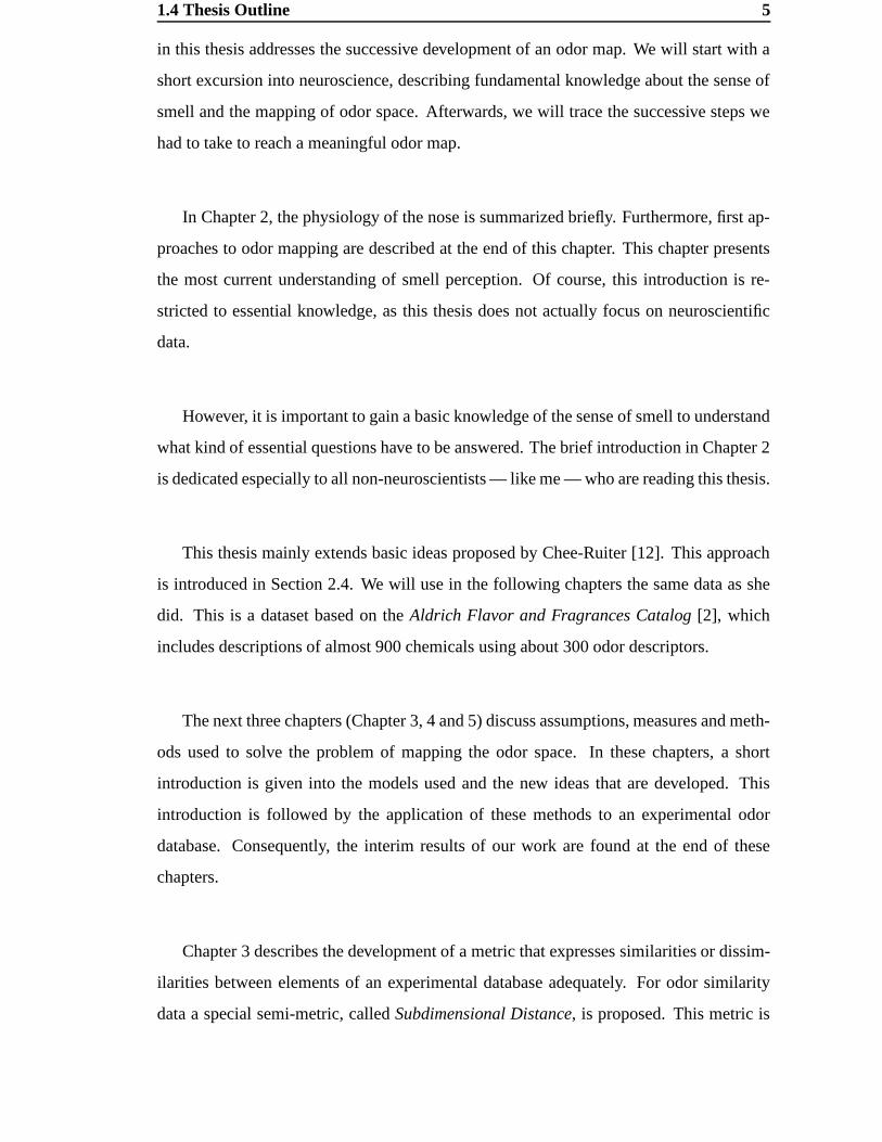
Figure 1.1: Data flow through mapping infrastructure.
found to be the most satisfying intuitively. Also, the independence of our approach of the
quality of psychophysical data is emphasized. Using this specially designed metric, we
obtain a dissimilarity estimate of the odor data, namely a ��������� dissimilarity matrix (see
Figure 1.1).
In Figure 1.1, the data flow from the raw data to the odor map is shown. � experi-
mental observation vectors are given that have features each. We will derive a �������dissimilarity matrix out of these feature vectors using the subdimensional distance. There
is a well-known numerical method to reconstruct metric points from a dissimilarity (dis-
tance) matrix. This method is called Multidimensional Scaling (MDS).
In Chapter 4, MDS is presented. The main idea is just to ignore whatever structure
might underlie the odor space data and instead to find the closest � -dimensional Euclidean
representation of the given dissimilarity matrix.
The odor space was found to be too complex to derive a map out of the MDS points
directly. This is because � , the dimension of the best Euclidean representation, is much
bigger than 2. If � had been 2 this thesis would have ended at this point. As it stands, how-
ever, we need a visualization technique for high-dimensional spaces, and so in Chapter
5, we apply a well-known method for topology-conserving data display, so-called Self-
organizing maps (SOMs).
In Chapter 6, we give a comprehensive summary of these results as well as a motiva-
tion of how the resulting maps can be used to test existing hypotheses. We will answer the
question of how the odors apple, banana and cherry are ordered in odor space. Further-
more, we will compare our map with existing approaches. Connections to Chee-Ruiter’s

1.4 Thesis Outline 7
directed graph will be shown.
We found evidence to support the so-called ecoproximity hypothesis. This is a hypoth-
esis about the role of key atoms in the environment for odor perception. This hypothesis
and the evidence that we found will be presented at the end of this chapter.
In the last chapter of this thesis, the infrastructure used to generate the map and the
results will be discussed. Finally, we will end the discussion with an outlook on potential
projects and future work.
C H A P T E R 2
Smell (Olfaction)
Anything that has a smell constantly evaporates tiny quantities of molecules that cause the
smell perception, so-called odorants, into the surrounding air. Therefore, the air is filled
with a mixture of different odorants, whether they were evaporated by a beautiful rose or
a rotting fish. These molecules are tiny, mostly invisible and chemically highly reactive.
A sensor that is capable of detecting such molecules is called a “chemical sensor”. Thus
the nose is a chemical sensor and the sense of smell is a chemical sense.
Even though most human beings are not actively conscious of their sense of smell, it
is the main sense for most mammals. They identify essential things like food, enemies or
even sexual partners using their nose. Odorants are able to influence our mood and can
trigger discomfort, sympathy as well as refusal. They might even influence our sexual
feelings, since each individual has an unique, genetically biased smell. So for humans, it
seems to be very likely that from an evolutionary point of view the nose played an impor-
tant role and probably still does so. Wells and Hepper [53] have drawn attention to the
often overlooked presence of our sense of smell. They tested dog owners for their ability
to identify individual dogs by their smell. Interestingly, � ������ of the participants were
able to recognize the odor of their own dog.
Mammals can distinguish a tremendous number of odorants, e.g. humans are able
to differentiate (depending upon training) around 10,000 of these odorous chemicals [4].
A smell sensation, a so-called odor (e.g. floral), can be perceived even in a very low
Smell (Olfaction) 9
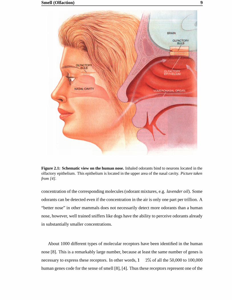
Figure 2.1: Schematic view on the human nose. Inhaled odorants bind to neurons located in theolfactory epithelium. This epithelium is located in the upper area of the nasal cavity. Picture takenfrom [4].
concentration of the corresponding molecules (odorant mixtures, e.g. lavender oil). Some
odorants can be detected even if the concentration in the air is only one part per trillion. A
“better nose” in other mammals does not necessarily detect more odorants than a human
nose, however, well trained sniffers like dogs have the ability to perceive odorants already
in substantially smaller concentrations.
About 1000 different types of molecular receptors have been identified in the human
nose [8]. This is a remarkably large number, because at least the same number of genes is
necessary to express these receptors. In other words, ������� of all the 50,000 to 100,000
human genes code for the sense of smell [8], [4]. Thus these receptors represent one of the
10 Smell (Olfaction)
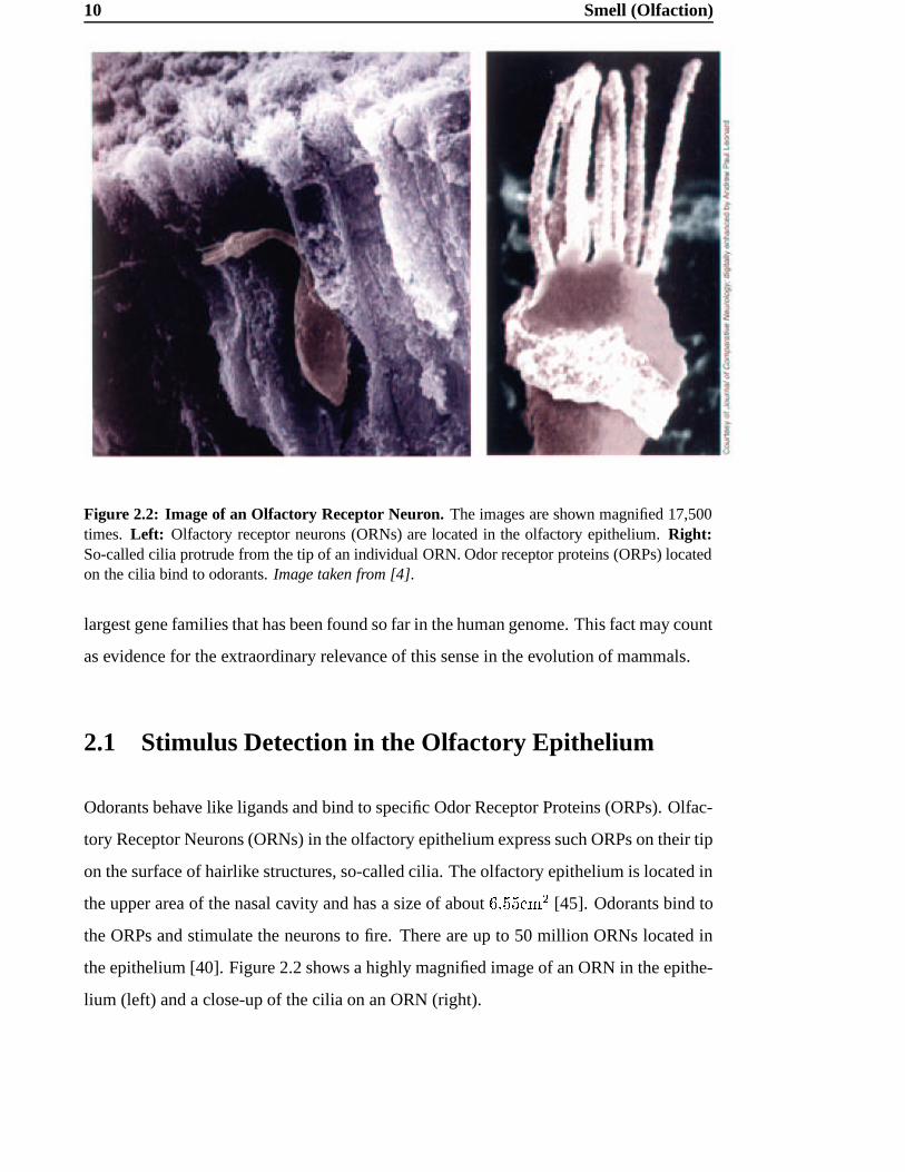
Figure 2.2: Image of an Olfactory Receptor Neuron. The images are shown magnified 17,500times. Left: Olfactory receptor neurons (ORNs) are located in the olfactory epithelium. Right:So-called cilia protrude from the tip of an individual ORN. Odor receptor proteins (ORPs) locatedon the cilia bind to odorants. Image taken from [4].
largest gene families that has been found so far in the human genome. This fact may count
as evidence for the extraordinary relevance of this sense in the evolution of mammals.
2.1 Stimulus Detection in the Olfactory Epithelium
Odorants behave like ligands and bind to specific Odor Receptor Proteins (ORPs). Olfac-
tory Receptor Neurons (ORNs) in the olfactory epithelium express such ORPs on their tip
on the surface of hairlike structures, so-called cilia. The olfactory epithelium is located in
the upper area of the nasal cavity and has a size of about ������������� [45]. Odorants bind to
the ORPs and stimulate the neurons to fire. There are up to 50 million ORNs located in
the epithelium [40]. Figure 2.2 shows a highly magnified image of an ORN in the epithe-
lium (left) and a close-up of the cilia on an ORN (right).
2.2 Signal Processing in the Olfactory Bulb 11
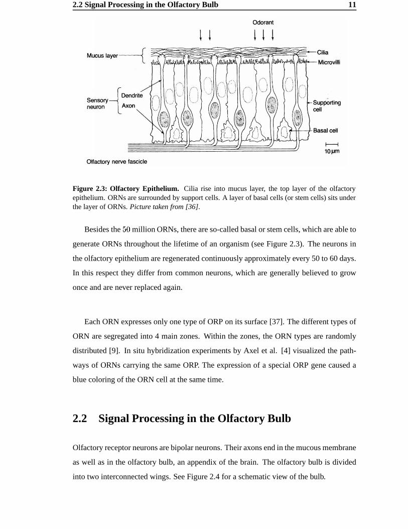
Figure 2.3: Olfactory Epithelium. Cilia rise into mucus layer, the top layer of the olfactoryepithelium. ORNs are surrounded by support cells. A layer of basal cells (or stem cells) sits underthe layer of ORNs. Picture taken from [36].
Besides the �! million ORNs, there are so-called basal or stem cells, which are able to
generate ORNs throughout the lifetime of an organism (see Figure 2.3). The neurons in
the olfactory epithelium are regenerated continuously approximately every 50 to 60 days.
In this respect they differ from common neurons, which are generally believed to grow
once and are never replaced again.
Each ORN expresses only one type of ORP on its surface [37]. The different types of
ORN are segregated into 4 main zones. Within the zones, the ORN types are randomly
distributed [9]. In situ hybridization experiments by Axel et al. [4] visualized the path-
ways of ORNs carrying the same ORP. The expression of a special ORP gene caused a
blue coloring of the ORN cell at the same time.
2.2 Signal Processing in the Olfactory Bulb
Olfactory receptor neurons are bipolar neurons. Their axons end in the mucous membrane
as well as in the olfactory bulb, an appendix of the brain. The olfactory bulb is divided
into two interconnected wings. See Figure 2.4 for a schematic view of the bulb.
12 Smell (Olfaction)
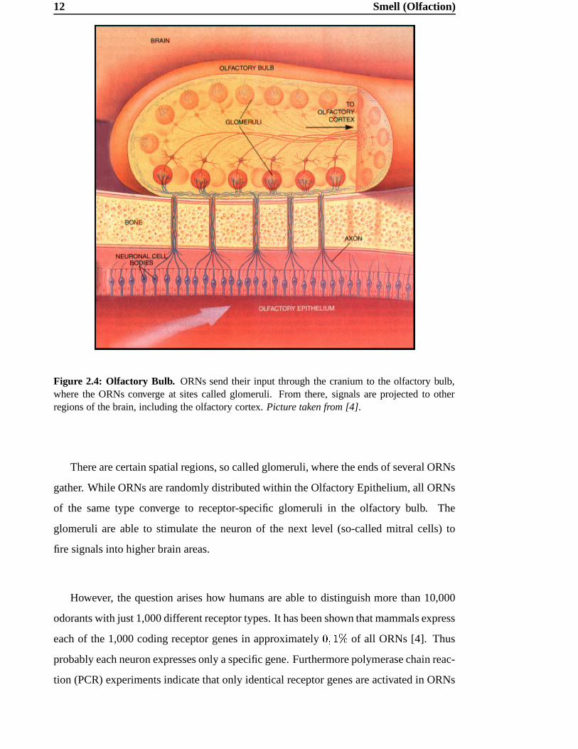
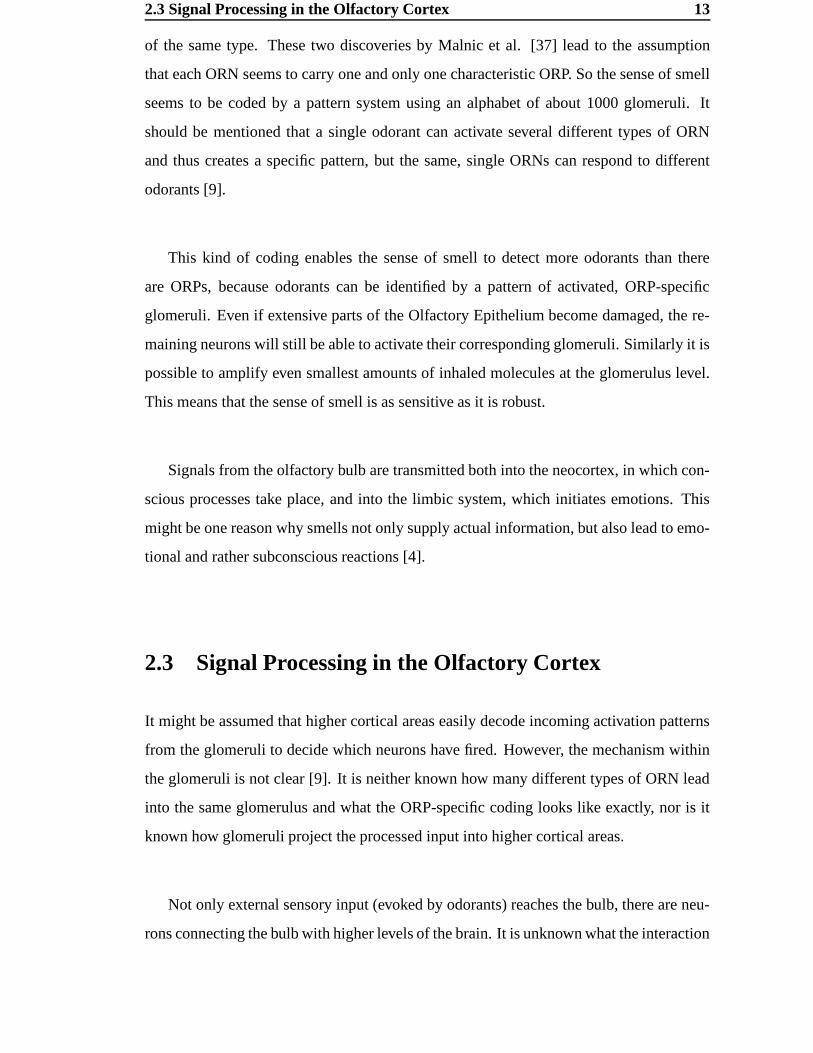
Figure 2.4: Olfactory Bulb. ORNs send their input through the cranium to the olfactory bulb,where the ORNs converge at sites called glomeruli. From there, signals are projected to otherregions of the brain, including the olfactory cortex. Picture taken from [4].
There are certain spatial regions, so called glomeruli, where the ends of several ORNs
gather. While ORNs are randomly distributed within the Olfactory Epithelium, all ORNs
of the same type converge to receptor-specific glomeruli in the olfactory bulb. The
glomeruli are able to stimulate the neuron of the next level (so-called mitral cells) to
fire signals into higher brain areas.
However, the question arises how humans are able to distinguish more than 10,000
odorants with just 1,000 different receptor types. It has been shown that mammals express
each of the 1,000 coding receptor genes in approximately �"#�$� of all ORNs [4]. Thus
probably each neuron expresses only a specific gene. Furthermore polymerase chain reac-
tion (PCR) experiments indicate that only identical receptor genes are activated in ORNs
2.3 Signal Processing in the Olfactory Cortex 13
of the same type. These two discoveries by Malnic et al. [37] lead to the assumption
that each ORN seems to carry one and only one characteristic ORP. So the sense of smell
seems to be coded by a pattern system using an alphabet of about 1000 glomeruli. It
should be mentioned that a single odorant can activate several different types of ORN
and thus creates a specific pattern, but the same, single ORNs can respond to different
odorants [9].
This kind of coding enables the sense of smell to detect more odorants than there
are ORPs, because odorants can be identified by a pattern of activated, ORP-specific
glomeruli. Even if extensive parts of the Olfactory Epithelium become damaged, the re-
maining neurons will still be able to activate their corresponding glomeruli. Similarly it is
possible to amplify even smallest amounts of inhaled molecules at the glomerulus level.
This means that the sense of smell is as sensitive as it is robust.
Signals from the olfactory bulb are transmitted both into the neocortex, in which con-
scious processes take place, and into the limbic system, which initiates emotions. This
might be one reason why smells not only supply actual information, but also lead to emo-
tional and rather subconscious reactions [4].
2.3 Signal Processing in the Olfactory Cortex
It might be assumed that higher cortical areas easily decode incoming activation patterns
from the glomeruli to decide which neurons have fired. However, the mechanism within
the glomeruli is not clear [9]. It is neither known how many different types of ORN lead
into the same glomerulus and what the ORP-specific coding looks like exactly, nor is it
known how glomeruli project the processed input into higher cortical areas.
Not only external sensory input (evoked by odorants) reaches the bulb, there are neu-
rons connecting the bulb with higher levels of the brain. It is unknown what the interaction
14 Smell (Olfaction)
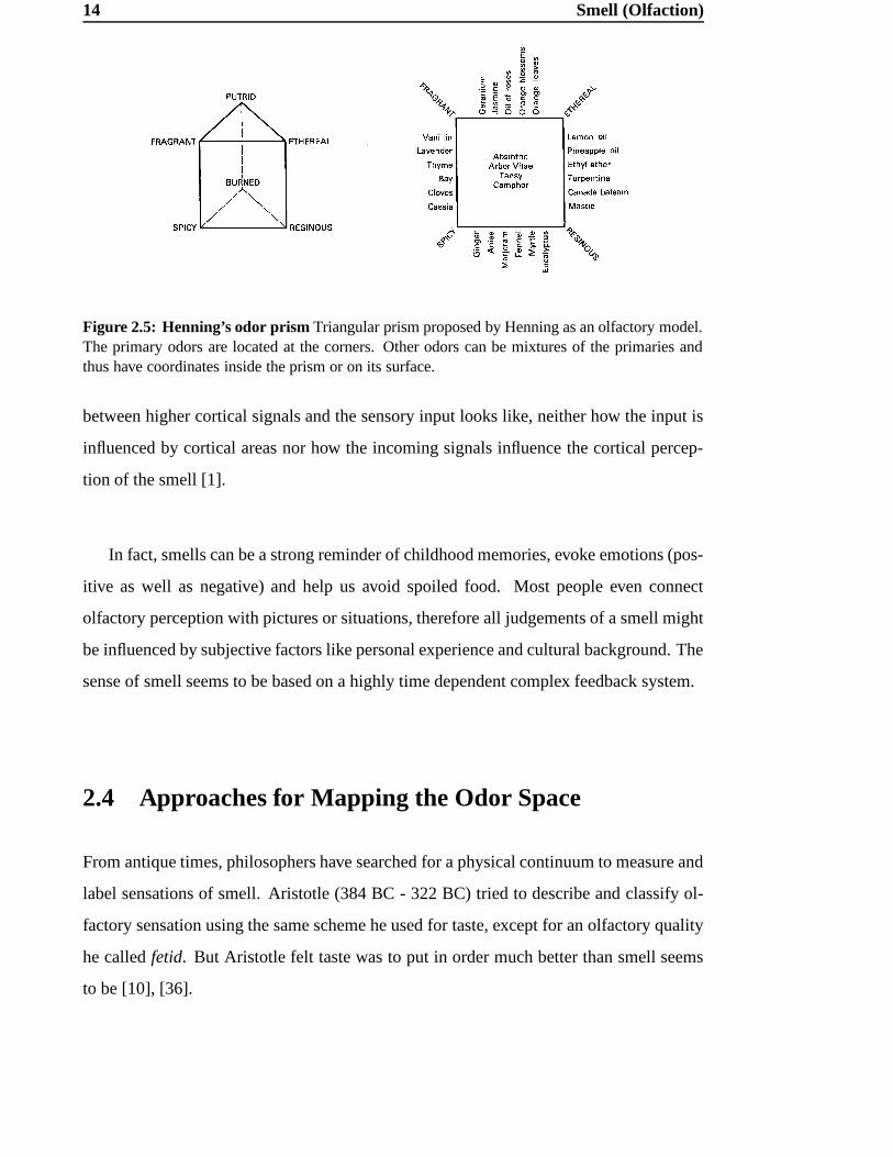
Figure 2.5: Henning’s odor prism Triangular prism proposed by Henning as an olfactory model.The primary odors are located at the corners. Other odors can be mixtures of the primaries andthus have coordinates inside the prism or on its surface.
between higher cortical signals and the sensory input looks like, neither how the input is
influenced by cortical areas nor how the incoming signals influence the cortical percep-
tion of the smell [1].
In fact, smells can be a strong reminder of childhood memories, evoke emotions (pos-
itive as well as negative) and help us avoid spoiled food. Most people even connect
olfactory perception with pictures or situations, therefore all judgements of a smell might
be influenced by subjective factors like personal experience and cultural background. The
sense of smell seems to be based on a highly time dependent complex feedback system.
2.4 Approaches for Mapping the Odor Space
From antique times, philosophers have searched for a physical continuum to measure and
label sensations of smell. Aristotle (384 BC - 322 BC) tried to describe and classify ol-
factory sensation using the same scheme he used for taste, except for an olfactory quality
he called fetid. But Aristotle felt taste was to put in order much better than smell seems
to be [10], [36].
2.4 Approaches for Mapping the Odor Space 15
Later, in the �% �&(' and �%)�&(' century, scientists tried to group odors into different classes,
just as animal and plant species are classified. Linnaeus (1752) grouped odors into seven
classes: aromatic, fragrant, ambrosial, alliaceous, hircine, repulsive and nauseous. A re-
fined version of this classification by Zwaardemaker (1895) remained accepted until well
into the �! &(' century. These early models were based on personal experience rather than
on experimental data [10].
Henning [21] tried to define primary odors experimentally. He proposed a prism with
six corners, labeled as putrid, fragrant, spicy, resinous and ethereal (see Figure 2.5). So
each odor would occupy a certain position in the prism, corresponding to its resemblance
to the primary odors. For example the odor thyme would probably be located between
fragrant and spicy. However, experimental subjects produced great variations in where
on the prism different odors are placed, so Henning’s theory eventually fell out of favor
[36].
In 1968 Woskow [56] applied an early multidimensional scaling (MDS) method to
psychophysical data, assuming that his data were metric. He directly derived similarities
from a matrix of ���+*,�!� odorants. The method yielded a three-dimensional space, but this
surprisingly small dimension could be caused by his small set of odorants.
Schiffman [46] reanalyzed Woskows data using a nonmetric MDS, since there is no a pri-
ori reason to assume that the data are metric. She found that no single physicochemical
parameter could be used individually to predict odor quality.
In Addition to these physicochemical maps, several empirical approaches have been
widely used by the perfume industry. In all cases, two- or three-dimensional spaces are
proposed. However, the scientific basis leading to these representations remains unclear.
It might be supposed that in most cases these models are empirical categorizations rather
than scientifically validated olfactory maps.
But even today scientists must choose their stimuli based largely on their personal
experience. There is no guarantee that the chosen stimuli are able to span the “olfactory
16 Smell (Olfaction)
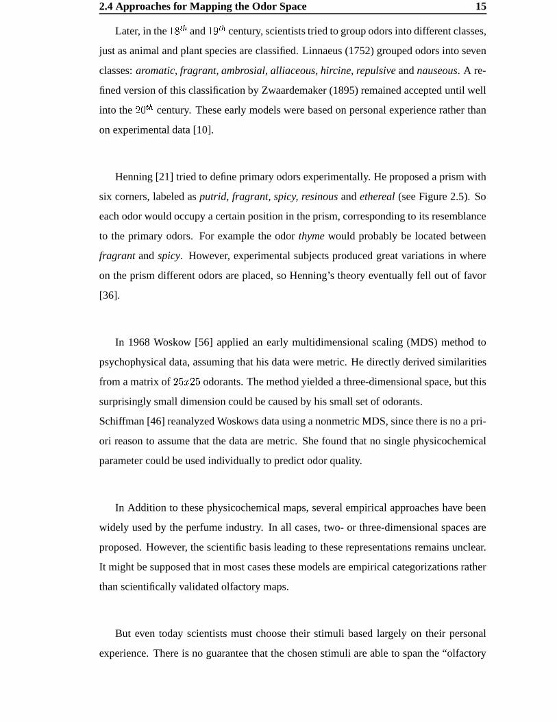
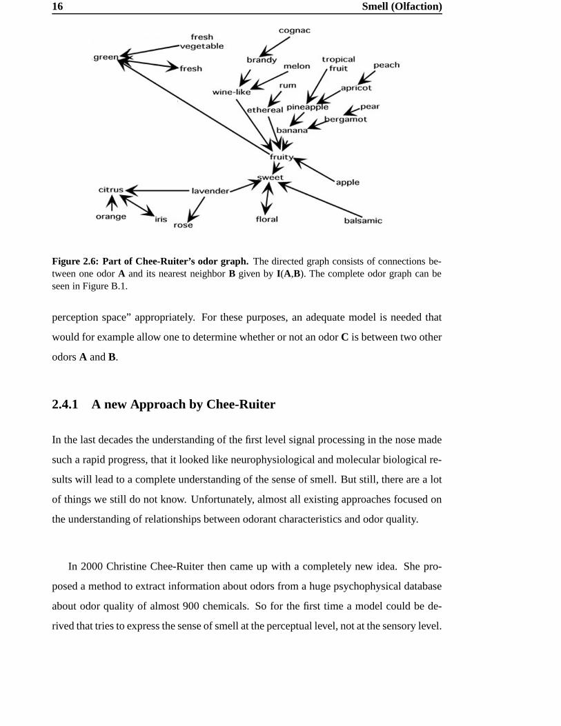
Figure 2.6: Part of Chee-Ruiter’s odor graph. The directed graph consists of connections be-tween one odor A and its nearest neighbor B given by I(A,B). The complete odor graph can beseen in Figure B.1.
perception space” appropriately. For these purposes, an adequate model is needed that
would for example allow one to determine whether or not an odor C is between two other
odors A and B.
2.4.1 A new Approach by Chee-Ruiter
In the last decades the understanding of the first level signal processing in the nose made
such a rapid progress, that it looked like neurophysiological and molecular biological re-
sults will lead to a complete understanding of the sense of smell. But still, there are a lot
of things we still do not know. Unfortunately, almost all existing approaches focused on
the understanding of relationships between odorant characteristics and odor quality.
In 2000 Christine Chee-Ruiter then came up with a completely new idea. She pro-
posed a method to extract information about odors from a huge psychophysical database
about odor quality of almost 900 chemicals. So for the first time a model could be de-
rived that tries to express the sense of smell at the perceptual level, not at the sensory level.
2.4 Approaches for Mapping the Odor Space 17
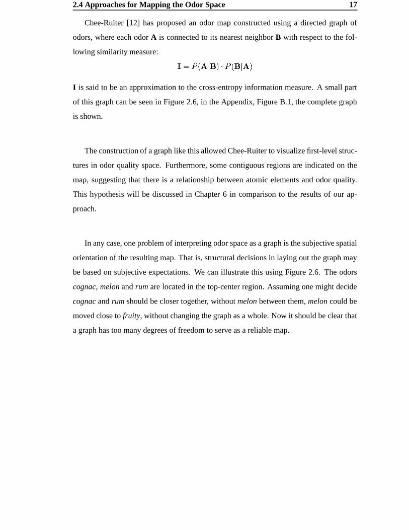
Chee-Ruiter [12] has proposed an odor map constructed using a directed graph of
odors, where each odor A is connected to its nearest neighbor B with respect to the fol-
lowing similarity measure: - .0/ �214365��87 / ��59361:�I is said to be an approximation to the cross-entropy information measure. A small part
of this graph can be seen in Figure 2.6, in the Appendix, Figure B.1, the complete graph
is shown.
The construction of a graph like this allowed Chee-Ruiter to visualize first-level struc-
tures in odor quality space. Furthermore, some contiguous regions are indicated on the
map, suggesting that there is a relationship between atomic elements and odor quality.
This hypothesis will be discussed in Chapter 6 in comparison to the results of our ap-
proach.
In any case, one problem of interpreting odor space as a graph is the subjective spatial
orientation of the resulting map. That is, structural decisions in laying out the graph may
be based on subjective expectations. We can illustrate this using Figure 2.6. The odors
cognac, melon and rum are located in the top-center region. Assuming one might decide
cognac and rum should be closer together, without melon between them, melon could be
moved close to fruity, without changing the graph as a whole. Now it should be clear that
a graph has too many degrees of freedom to serve as a reliable map.
C H A P T E R 3
Quality and Comparison of Experimental Data
In this chapter, we want to discuss how to extract odor perception information from ex-
perimental data. The topic of this chapter is thus twofold. First, we have to talk about
psychophysical experiments; then, we will address the comparison of experimental re-
sults.
Modern psychophysics is devoted to quantifying the relationship between a given
stimulus and the triggered sensation, usually for the purpose of describing the processes
underlying perception [36].
These relationships are documented using so-called observation vectors (or feature
vectors). Think of an experiment testing the odor quality values of odorants. Let * be one
of the stimuli, say ; -Toluenethiol. This odorant is often used to give canned soups the
typical aroma of meat. Even in low concentrations, it smells very intense and unpleasant,
with a slightly sulfurous nuance. The subjects now have to smell this substance among
other substances several times and have to judge the odor quality. This is done by fill-
ing out a data sheet for each stimulus. The sheet consists of a set of odor descriptors,
e.g. fruity; the descriptors matching the subject’s perception are marked. The classical
psychophysical approach averages the results and extracts feature vectors using a certain
threshold. If unpleasant is descriptor < for example, then the < -th entry of observation
vector =?> would presumably be set to one (if ; -Toluenethiol is being profiled).
3.1 Distances and Similarities 19
3.1 Distances and Similarities
An observation vector =@> that is gained in such an experiment quantifies the perceptive
reactions to a stimulus * , often in binary quantization. We are usually trying to put two
given observation vectors =@> and =?A with=?> . ��; > B "#�#�#��"C; >D �FEG" =?A . �2; A B "H�#�#�H"I; AD �JE (1.1)
in one context. This means that we are comparing two observations with each one another
to obtain information about how they relate, how similar or dissimilar they are. The main
problem in measuring similarity is to devise an appropriate distance function KL�2=M>�"I=?A��that yields intuitively satisfying results for the dissimilarities (the distances) of =M> and=?A . That is, the dissimilarity measure should yield a high number when the two obser-
vations differ in a high number of features (parameters) and a lower number otherwise.
Conversely, we would expect a similarity measure to produce a low value for a high num-
ber of equal features.
The term distance is often used to describe precisely the differences of actual mea-
surements, while “dissimilarity” might be an estimation of a distance we are not able to
measure physically. But distance can be interpreted as a dissimilarity as well. Basically
distance and similarity are reciprocal concepts.
To interpret dissimilarities in a geometrical sense, e.g. to derive a map out of an
existing dissimilarity matrix, it is reasonable to interpret dissimilarities as distances in a
metric space. This enables us to measure distances between two observations like on a
city map. On the other hand, especially when dealing with highly complex objects, it
is not always possible to express similarities with a mathematically stringent metric. To
clarify this practical problem, we will now give a definition of a mathematical metric.
Definition 3.1.1 Metric. Let KL�2=N>�"C=?AH� be a distance function that defines the dis-
tance of an observation =@> and an observation =@A . If this distance function fulfills the
20 Quality and Comparison of Experimental Data
following conditions, it is called a metric.��KL�2=?>�"I=?A#�POQ R� S �2KL��=?>�"C=?AH� . UT * .WV � (positive definiteness) (1.2)KL�2=?>�"I=?A#� . K,��=?A$"C=?>$� (symmetry) (1.3)KL�2=?>R"I=NXY�[ZQKL�2=?>�"I=?A#��\]KL�2=?A+"C=NXY� (triangle inequality) (1.4)
Definition 3.1.2 Semi-Metric and Asymmetric Metric
A semi-metric does not fulfill the triangle inequality, but is positive definite and symmet-
ric, i.e. it fulfills the conditions (1.2) and (1.3) of a metric.
An asymmetric metric is positive definite and fulfills the triangle inequality but is not
symmetric, i.e. it fulfills only the conditions (1.2) and (1.4) of a metric.
It should be mentioned, that semi-metrics as well as asymmetric metrics are not suit-
able for interpretation as describing a geometrical space. Under a semi-metric the direct
connection between two points does not have to be the shortest path, and under an asym-
metric metric, the route from one point to another might be shorter or longer than the
route back. Nevertheless, semi- and asymmetric metrics might be more suitable than pure
metrics for describing dissimilarities because they are less restricted and, a priori, an ex-
perimental feature space does not necessarily have to satisfy the conditions for a metric.
On the contrary, similarity has been shown in several experiments to be very asymmetric.
For example, subjects said that the number 99 was very similar to the number 100, but
balked at describing 100 as very similar to 99 [39].
An important quantifier for an observation vector in the context of different metrics is
its stuffing, so let us define this term in the following.
The stuffing of an observation vector =@> is the number of components that differ from
zero. For binary vectors, this can be expressed as a sum over all components:
3.2 Typical Dissimilarity Measures 21
Definition 3.1.3 Stuffing of observation vectors.^`_Iacbed�f ��=?>$�Pg .0h =?>ig .kjLl ; >l (1.5)
3.2 Typical Dissimilarity Measures
There are many different metrics for expressing the distance between two objects. There-
fore, the importance of choosing a suitable metric should be emphasized again. This is
essential for a meaningful description of a data space. It should be clear that a wrong
description of facts leads to wrong results and cannot be compensated in later steps. We
have to admit though that it is not very easy to prove “correctness” in this context.
A reasonable approach is to test the most commonly used metrics and evaluate them
for specific data. Based on these results, one can develop one’s own (specially adapted)
measure, to obtain a measure that is as intuitively satisfying as possible. Consequently,
we will start by describing some common metrics, and afterwards a short derivation of
our new dissimilarity measure will be given.
The first metric to be defined is the so-called Minkowski Metric. It is the general case
of a set of typical and familiar metrics. The basic structure of these metrics is defined as
follows:
Definition 3.2.1 Minkowski Metric.
KRm?��=?>�"C=?AH�[g .on�j,l 36; >l ��; Al 3 p%q B2r p "Cs9Ot��"Ysvu9w (2.1)
As a special case of the Minkowski Metric with s . � , the city-block (or Manhattan)
distance Kyx between two observations =@> and =?A is defined as follows:
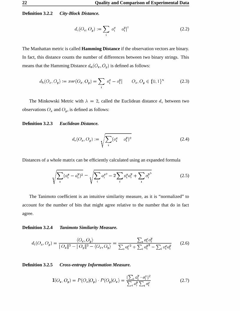
22 Quality and Comparison of Experimental Data
Definition 3.2.2 City-Block Distance.KRxz�2=?>!"C=?AH�[g .0j,l 36; >l ��; Al 3 B (2.2)
The Manhattan metric is called Hamming Distance if the observation vectors are binary.
In fact, this distance counts the number of differences between two binary strings. This
means that the Hamming Distance K ' �2=?>�"C=?A�� is defined as follows:K ' ��=?>�"C=?AH�[g . *L;+{��2=?>!"C=?AH� .0j,l 36; >l ��; Al 3 =?>R"C=?A?u4|+ �"#�!} D (2.3)
The Minkowski Metric with s . � , called the Euclidean distance Kc~ between two
observations =N> and =?A , is defined as follows:
Definition 3.2.3 Euclidean Distance.KR~#��=?>�"C=?AH�Pg . j,l �2; >l ��; Al � � (2.4)
Distances of a whole matrix can be efficiently calculated using an expanded formulaj�l �2; >l ��; Al � � . j,l ; >l � �]� jLl ; >l ; Al \ j,l ; Al � (2.5)
The Tanimoto coefficient is an intuitive similarity measure, as it is “normalized” to
account for the number of bits that might agree relative to the number that do in fact
agree.
Definition 3.2.4 Tanimoto Similarity Measure.K & ��=?>�"C=?AH� . � =?>�"I=?A#�� =?> � � \ � =?A � � � � =?>�"C=?AH� . � l ; >l ; Al� l ; >l ��\ � l ; Al � � � l ; >l ; Al (2.6)
Definition 3.2.5 Cross-entropy Information Measure.- �2=?>!"C=?A�� .W/ �2=?>�3 =?AH��7 / ��=?AR36=?>$� . � � l ; Al 7%; >l ���� l ; Al � l ; >l (2.7)
3.3 Quality of Odor Dissimilarity Data 23
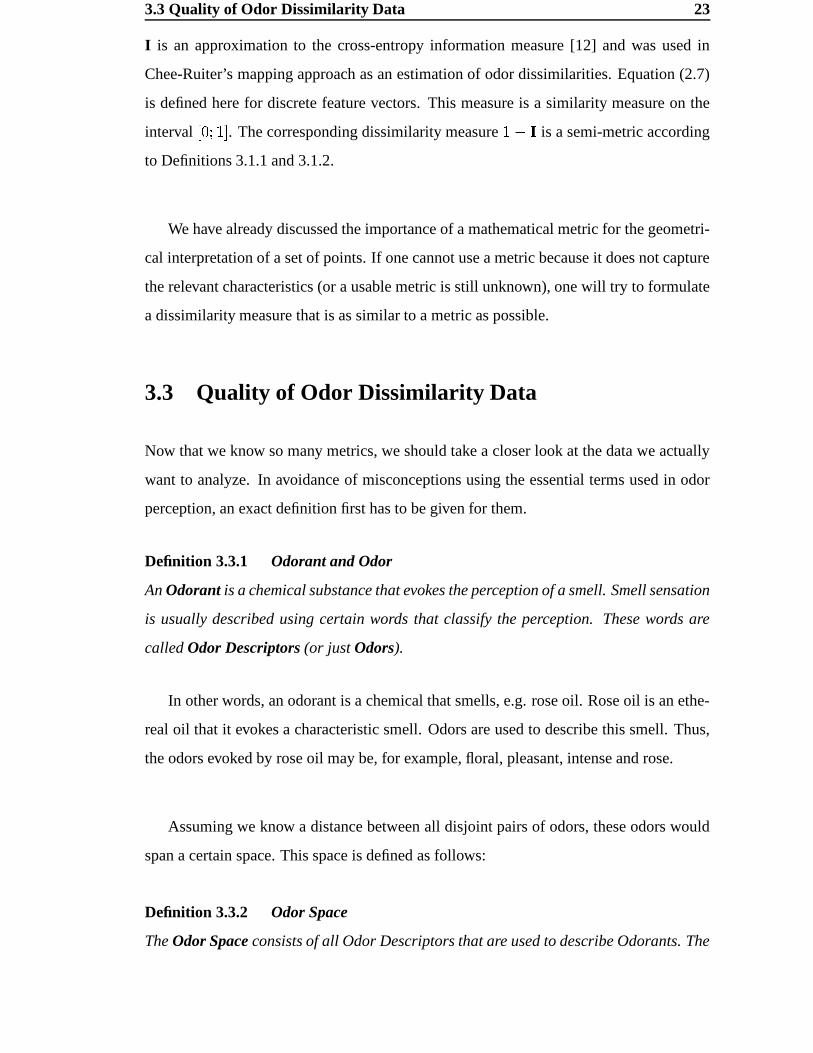
I is an approximation to the cross-entropy information measure [12] and was used in
Chee-Ruiter’s mapping approach as an estimation of odor dissimilarities. Equation (2.7)
is defined here for discrete feature vectors. This measure is a similarity measure on the
interval �� ��#��� . The corresponding dissimilarity measure ��� -is a semi-metric according
to Definitions 3.1.1 and 3.1.2.
We have already discussed the importance of a mathematical metric for the geometri-
cal interpretation of a set of points. If one cannot use a metric because it does not capture
the relevant characteristics (or a usable metric is still unknown), one will try to formulate
a dissimilarity measure that is as similar to a metric as possible.
3.3 Quality of Odor Dissimilarity Data
Now that we know so many metrics, we should take a closer look at the data we actually
want to analyze. In avoidance of misconceptions using the essential terms used in odor
perception, an exact definition first has to be given for them.
Definition 3.3.1 Odorant and Odor
An Odorant is a chemical substance that evokes the perception of a smell. Smell sensation
is usually described using certain words that classify the perception. These words are
called Odor Descriptors (or just Odors).
In other words, an odorant is a chemical that smells, e.g. rose oil. Rose oil is an ethe-
real oil that it evokes a characteristic smell. Odors are used to describe this smell. Thus,
the odors evoked by rose oil may be, for example, floral, pleasant, intense and rose.
Assuming we know a distance between all disjoint pairs of odors, these odors would
span a certain space. This space is defined as follows:
Definition 3.3.2 Odor Space
The Odor Space consists of all Odor Descriptors that are used to describe Odorants. The
24 Quality and Comparison of Experimental Data
position of Odor Descriptors in this space is determined by their relationships to each
other.
The dimensionality and the metric of this space or anything else about the structure of
this space is unknown.
To illustrate what a typical dataset looks like, let us examine a tiny database consisting
of only three odorants: hexyl butyrate, methyl-2-methylbutyrate and 6-amyl- � -pyrone.
And furthermore let us assume, these chemicals are characterized (e.g. by an objective
psychophysical experiment) by the following profiles:
hexyl butyrate g sweet – fruity – pineapple
methyl-2-methylbutyrate g fruity – sweet – apple
6-amyl- � -pyrone g coconut – nutty – sweet
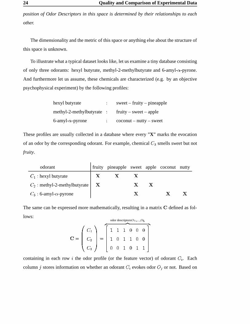
These profiles are usually collected in a database where every ”X” marks the evocation
of an odor by the corresponding odorant. For example, chemical ��� smells sweet but not
fruity.
odorant fruity pineapple sweet apple coconut nutty� B g hexyl butyrate � � �� � g methyl-2-methylbutyrate � � ��P��g 6-amyl- � -pyrone � � �The same can be expressed more mathematically, resulting in a matrix � defined as fol-
lows:
� . ����� � B� ��P��H���� . odor descriptors �L�F�6�6�6� � �c�� �H� ¡¢¢¢£ � � � � � � � � �
¤¦¥¥¥§containing in each row < the odor profile (or the feature vector) of odorant � l . Each
column ¨ stores information on whether an odorant � l evokes odor =ª© or not. Based on
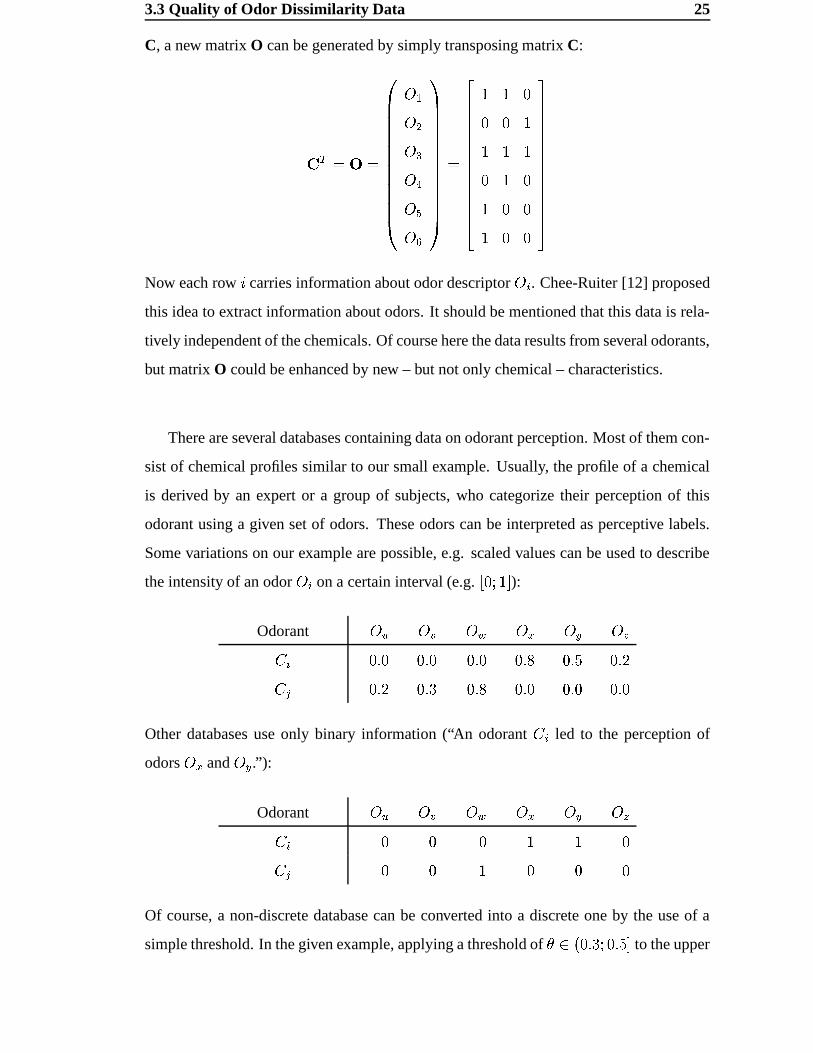
3.3 Quality of Odor Dissimilarity Data 25
C, a new matrix O can be generated by simply transposing matrix C:
�ME .t«¬. ��������������= B= �=N�=?=N®=N¯
�H�������������.
¡¢¢¢¢¢¢¢¢¢¢¢¢£� � �� � � � � �
¤¦¥¥¥¥¥¥¥¥¥¥¥¥§Now each row < carries information about odor descriptor = l . Chee-Ruiter [12] proposed
this idea to extract information about odors. It should be mentioned that this data is rela-
tively independent of the chemicals. Of course here the data results from several odorants,
but matrix O could be enhanced by new – but not only chemical – characteristics.
There are several databases containing data on odorant perception. Most of them con-
sist of chemical profiles similar to our small example. Usually, the profile of a chemical
is derived by an expert or a group of subjects, who categorize their perception of this
odorant using a given set of odors. These odors can be interpreted as perceptive labels.
Some variations on our example are possible, e.g. scaled values can be used to describe
the intensity of an odor = l on a certain interval (e.g. �� ��#�H� ):Odorant =N° =?± =?² =?> =?A =NX� l c�� ��� ��³ ��³ ���� ��´��µ© c�´� ���¶ ��³ ��³ ��³ ���
Other databases use only binary information (“An odorant � l led to the perception of
odors =N> and =?A .”):
Odorant =N° =?± =?² =?> =?A =NX� l � � �µ© � Of course, a non-discrete database can be converted into a discrete one by the use of a
simple threshold. In the given example, applying a threshold of ·¸u��2 c��¶��I ��´�$� to the upper
26 Quality and Comparison of Experimental Data
matrix would result the lower matrix.
We used a dataset based on the Aldrich Flavor and Fragrances Catalog [2], which
includes descriptions of 851 chemicals using 278 odor descriptors, mainly collected from
the primary sources [3] and [19]. This dataset has already been used for a first mapping
approach by Chee-Ruiter [12], as described already in Section 2.4. Although there are
other databases containing comparable data, e.g. Dravnieks [17], we will use the Aldrich
database in the following as the source of information for our mapping of the odor space.
The comparative evaluation of maps derived from different sources will not be discussed
in this thesis. Instead, we will focus on the introduction of an infrastructure for analyzing
olfactory perception databases in general.
3.3.1 Are these databases trustworthy?
First of all it should be clear that it is impossible to set up an objective psychophysical
experiment as long as we are not able to measure results physically. Thus, we can only
estimate the quality of these sets because we do not even know the correct similarity value
for a single pair of odors. And we have to expect a high vagueness in the correctness and
in the completeness of these profiles as well as a high variance, because every subject ex-
periences odorants differently. Finally, we cannot be even sure that odors that are chosen
are suitable. They are just words used to describe sensations evoked by odorants.
On the other hand, it can be expected that a chemical that is commonly characterized
as “nutty”, for example, will not be described as smelling like “apple”, neither by a
layperson nor by an expert. And only because a layperson is not as well educated for
describing his smell sensation, it does not mean that his/her nose is not able to detect fine
nuances in a discrimination experiment.
Dravnieks [16] was able to show that the information conveyed by odor descriptors
is stable. However, there might be a certain distortion, making the odors more dense in
familiar areas, like for example the description of fruity odorants. Especially these odors –
3.4 Estimating dissimilarities in the Odor Space 27
including hedonic values like “pleasant” and “unpleasant” – are often said to be cultural
or subjective in a certain way, for example, “green” is a typical odor that people might
interpret ambiguously.
The question arises how a potential map is influenced by these problems. Certainly a
map cannot become better than the data it relies on. But we want to introduce a depend-
able infrastructure to extract as much information as possible out of the databases. This
would mean that, given good data, we will be able to produce a good map.
Actually, it is not possible to gain access to human association without the use of
language. Wise et al.[54] tried to avoid the use of language, but experiments like this
cannot help in finding a unique set of odors, they are just helpful in measuring similarities
between odorants (chemicals) directly. This thesis will assume that the set of odors (here
Chee-Ruiter’s database [12]) is complete in terms of the knowledge acquired so far. The
question of how to define correctness for a set of odors has to be part of future work.
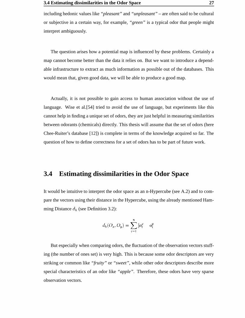
3.4 Estimating dissimilarities in the Odor Space
It would be intuitive to interpret the odor space as an n-Hypercube (see A.2) and to com-
pare the vectors using their distance in the Hypercube, using the already mentioned Ham-
ming Distance K ' (see Definition 3.2):K ' �2=?>!"C=?AH� . Dj l(¹ B 36; >l ��; Al 3But especially when comparing odors, the fluctuation of the observation vectors stuff-
ing (the number of ones set) is very high. This is because some odor descriptors are very
striking or common like “fruity” or “sweet”, while other odor descriptors describe more
special characteristics of an odor like “apple”. Therefore, these odors have very sparse
observation vectors.
28 Quality and Comparison of Experimental Data
0 50 100 150 200 2500
50
100
150
200
250stuffing of observation vectors
observation vector
num
ber
j of s
et e
lem
ents
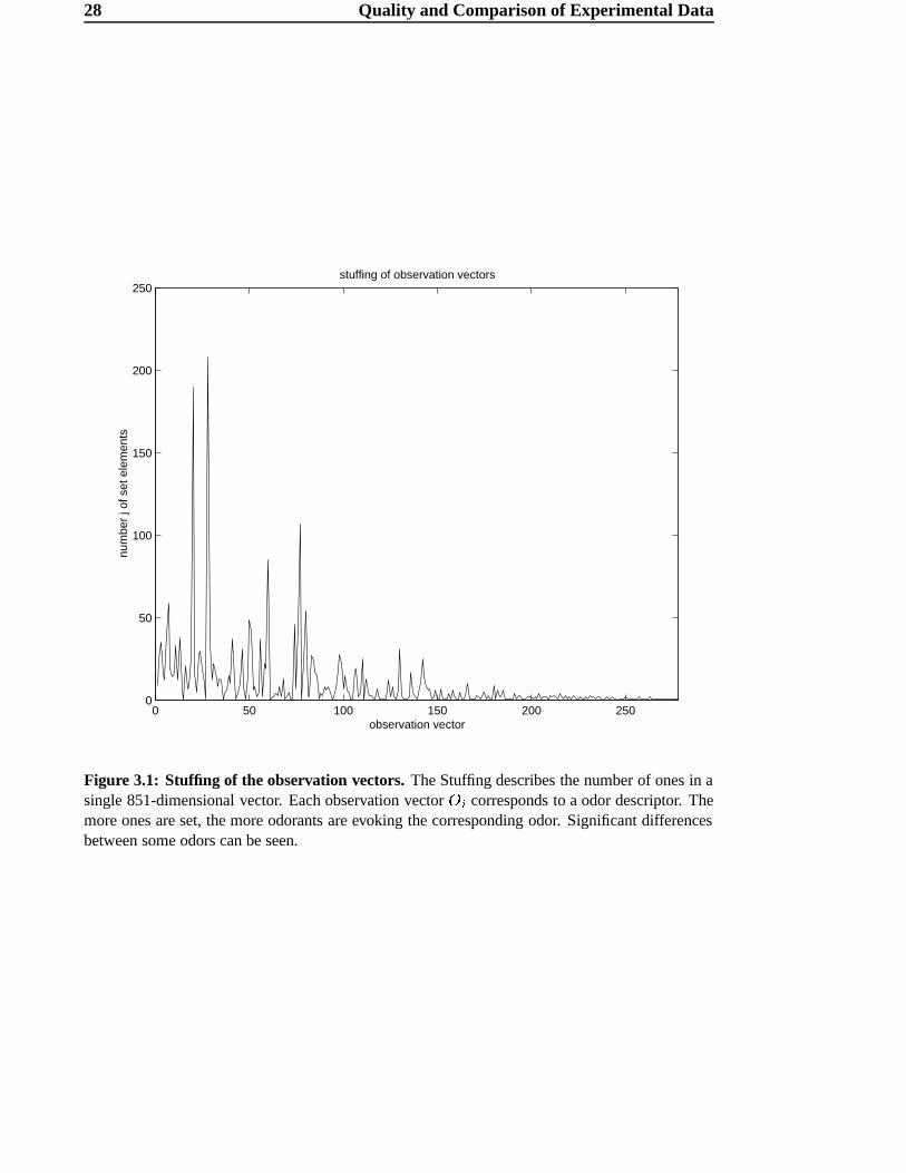
Figure 3.1: Stuffing of the observation vectors. The Stuffing describes the number of ones in asingle 851-dimensional vector. Each observation vector º l corresponds to a odor descriptor. Themore ones are set, the more odorants are evoking the corresponding odor. Significant differencesbetween some odors can be seen.
3.4 Estimating dissimilarities in the Odor Space 29
In Figure 3.1, the significant differences between common and special odors can be
seen. The average odor can be evoked by about eight odorants, but some are evoked
by several hundreds. This problem will be discussed in slightly more detail using the
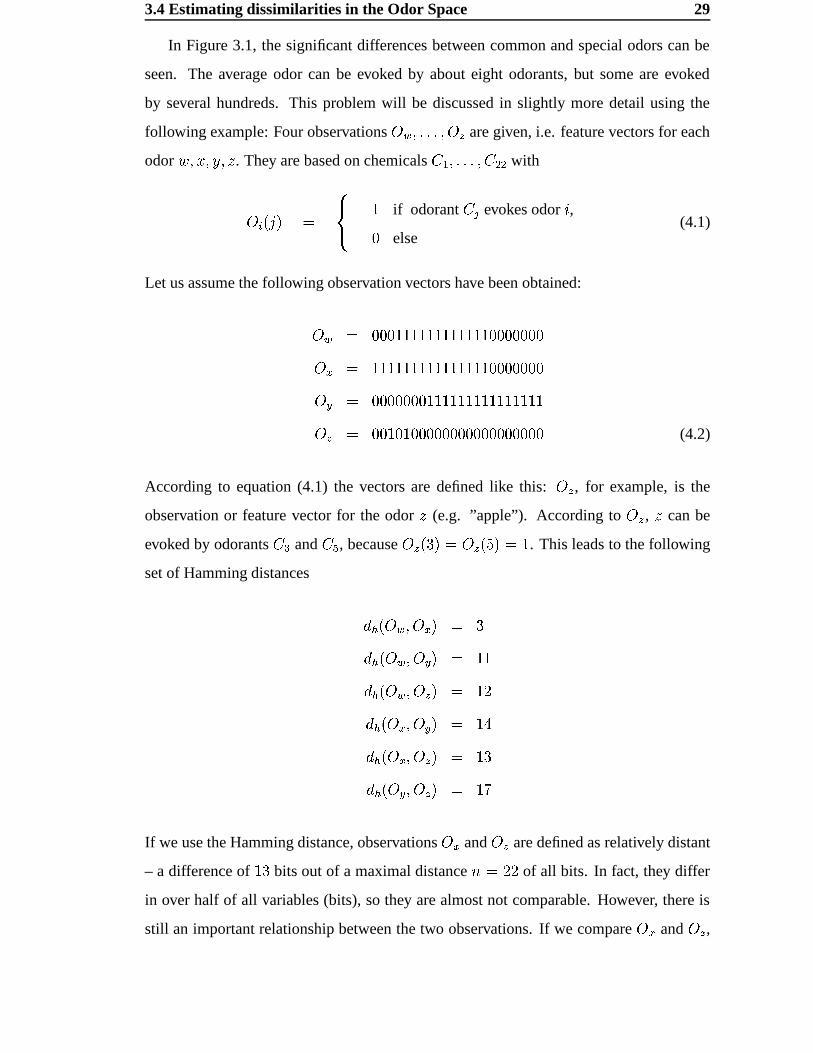
following example: Four observations =U²G"#�H�#�H"C=NX are given, i.e. feature vectors for each
odor »�"¼*8" V "C½ . They are based on chemicals � B "#�H�#�H"C� �J� with
= l �¾¨¿� . ÀÁ� � if odorant �µ© evokes odor < , else(4.1)
Let us assume the following observation vectors have been obtained:=?² . � ! ��������!���������!�����% � ! � � � � =?> . ���!���������!���������!�����% � ! � � � � =?A . � ! � � � � c���������!���������!���������=NX . � c�% ��% � ! � � � � ! � � � � ! � � � � (4.2)
According to equation (4.1) the vectors are defined like this: =MX , for example, is the
observation or feature vector for the odor ½ (e.g. ”apple”). According to =�X , ½ can be
evoked by odorants ��� and �P® , because =@X+��¶R� . =NX$�2��� . � . This leads to the following
set of Hamming distances K ' �2=?²G"C=?>$� . ¶K ' �2=?²G"C=?A�� . �!�K ' �2=?²G"C=NXY� . �%�K ' �2=?>R"C=?A�� . �HÃK ' ��=?>�"C=NXY� . �#¶K ' �2=?A+"C=NXY� . �%ÄIf we use the Hamming distance, observations =@> and =@X are defined as relatively distant
– a difference of �%¶ bits out of a maximal distance � . ��� of all bits. In fact, they differ
in over half of all variables (bits), so they are almost not comparable. However, there is
still an important relationship between the two observations. If we compare =M> and =NX ,
30 Quality and Comparison of Experimental Data
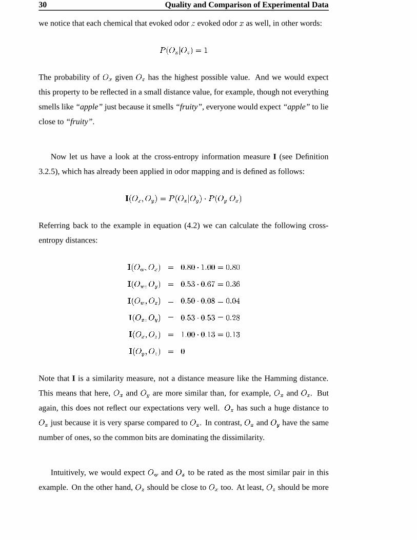
we notice that each chemical that evoked odor ½ evoked odor * as well, in other words:/ �2=?>c36=NXY� . �The probability of =N> given =@X has the highest possible value. And we would expect
this property to be reflected in a small distance value, for example, though not everything
smells like “apple” just because it smells “fruity”, everyone would expect “apple” to lie
close to “fruity”.
Now let us have a look at the cross-entropy information measure I (see Definition
3.2.5), which has already been applied in odor mapping and is defined as follows:- �2=?>�"I=?A#� .Å/ ��=?>�36=?AH��7 / �2=?AR3 =?>$�Referring back to the example in equation (4.2) we can calculate the following cross-
entropy distances: - ��=?²G"C=?>$� . ��³ � N7R���³ � . ��³ � - �2=?²G"C=?AH� . ����!¶N7$ ��³�RÄ . ��³¶��- �2=?²G"C=NXY� . ����! N7$ ��³ � . ��³ !Ã- ��=?>�"C=?AH� . ����!¶N7$ ����!¶ . ����! - �2=?>!"C=NXY� . ���³ � N7$ ��¾�%¶ . ��¾�%¶- �2=?A+"C=NXY� . Note that I is a similarity measure, not a distance measure like the Hamming distance.
This means that here, =N> and =?A are more similar than, for example, =@> and =NX . But
again, this does not reflect our expectations very well. =�X has such a huge distance to=?> just because it is very sparse compared to =@> . In contrast, =N> and =?A have the same
number of ones, so the common bits are dominating the dissimilarity.
Intuitively, we would expect =@² and =?> to be rated as the most similar pair in this
example. On the other hand, =UX should be close to =N> too. At least, =@X should be more
3.4 Estimating dissimilarities in the Odor Space 31
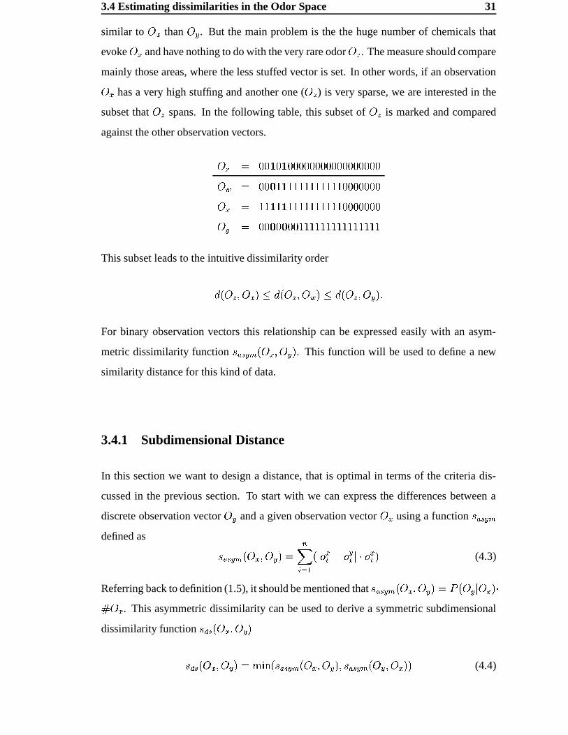
similar to =N> than =?A . But the main problem is the the huge number of chemicals that
evoke =?> and have nothing to do with the very rare odor =MX . The measure should compare
mainly those areas, where the less stuffed vector is set. In other words, if an observation=?> has a very high stuffing and another one ( =MX ) is very sparse, we are interested in the
subset that =@X spans. In the following table, this subset of =UX is marked and compared
against the other observation vectors.=NX . � ÇÆy ÇÆy � � ! � � � � ! � � � � ! � � � =?² . � �È��RÆÉ�����!���������!���% � � ! � � � =?> . ���RÆÉ�RÆÉ�����!���������!���% � � ! � � � =?A . � �È� �È� � ��!���������!���������!�������This subset leads to the intuitive dissimilarity orderKL��=NX#"C=?>$�[ZÅKL�2=NXH"C=?²,�PZQK,��=NX#"C=?AH�z�For binary observation vectors this relationship can be expressed easily with an asym-
metric dissimilarity function Ê%˼ÌÍA`mN�2=?>!"C=?AH� . This function will be used to define a new
similarity distance for this kind of data.
3.4.1 Subdimensional Distance
In this section we want to design a distance, that is optimal in terms of the criteria dis-
cussed in the previous section. To start with we can express the differences between a
discrete observation vector =@A and a given observation vector =@> using a function Ê%˼ÌÍA`mdefined as Ê%Ë`Ì�A�mN�2=?>�"I=?A#� . Dj l(¹ B �Y3 ; >l ��; Al 3$7$; >l � (4.3)
Referring back to definition (1.5), it should be mentioned that Ê�Ë`Ì�A�m@��=?>�"C=?AH� .0/ �2=?AR3 =?>$�Y7h =?> . This asymmetric dissimilarity can be used to derive a symmetric subdimensional
dissimilarity function Ê$Î�Ì��2=?>R"I=?A��Ê%Î�Ì��2=?>!"C=?AH� . �eÏ d �2Ê#˼ÌÍA`mN�2=?>R"I=?A��z"YÊ#Ë`Ì�A�m@��=?A�"I=?>$�¼� (4.4)
32 Quality and Comparison of Experimental Data
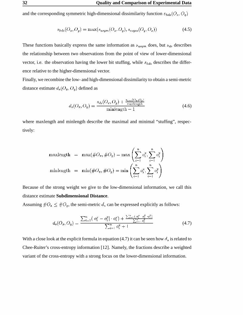
and the corresponding symmetric high-dimensional dissimilarity function Ê ' Î�Ìz�2=?>�"C=?A��Ê ' Î�Ì��2=?>�"I=?A#� . �ÑÐ+Ò��2Ê%Ë`Ì�A�mN�2=?>�"I=?A#�Y"YÊ#˼ÌÍA`m?��=?A�"I=?>$�¼� (4.5)
These functions basically express the same information as Ê�Ë`Ì�A�m does, but Ê#Î`Ì describes
the relationship between two observations from the point of view of lower-dimensional
vector, i.e. the observation having the lower bit stuffing, while Ê ' Î�Ì describes the differ-
ence relative to the higher-dimensional vector.
Finally, we recombine the low- and high-dimensional dissimilarity to obtain a semi-metric
distance estimate K¿Ì���=?>R"C=?A�� defined as
KyÌH��=?>�"C=?AH� . Ê#Î�Ì��2=?>�"I=?A#��\ ÌÔÓFÕ2Ö�× ��Ø�� ��Ù`ÚÛ8ÜÔÝ`Þ6ß�à¼áFâäã�eÏ dÇåäæ�dÇf!_Iç \Å� (4.6)
where maxlength and minlength describe the maximal and minimal “stuffing”, respec-
tively:
�ÑÐ+Ò åèæHdÇf!_¼ç . �ÑÐ$Òé� h =?>R" h =?AH� . �eÐ+Ò n Dj l(¹ B ; >l " Dj l(¹ B ; Al q�eÏ dÇåäæ�dÇf!_¼ç . �eÏ d � h =?>R" h =?AH� . �eÏ d n Dj l(¹ B ; >l " Dj l(¹ B ; Al qBecause of the strong weight we give to the low-dimensional information, we call this
distance estimate Subdimensional Distance.
Assuming h =?>iZ h =?A , the semi-metric K¿Ì can be expressed explicitly as follows:
KyÌ��2=?>�"I=?A#� . � Dl(¹ B �Y3 ; >l ��; Al 3$7%; >l ��\ëêNìí³î � ×äï ð Øí�ñ ð Ùí ï ò ð Ùí Úê ìí�î � ð Ùí� Dl¦¹ B ; >l \Å� (4.7)
With a close look at the explicit formula in equation (4.7) it can be seen how KÇÌ is related to
Chee-Ruiter’s cross-entropy information [12]. Namely, the fractions describe a weighted
variant of the cross-entropy with a strong focus on the lower-dimensional information.
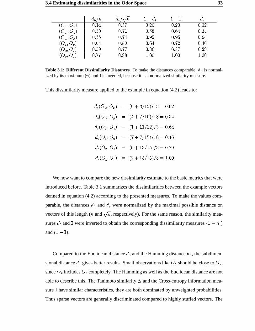
3.4 Estimating dissimilarities in the Odor Space 33K '%ó � Ky~ óyô � �õ�öK & �ª� - KyÌ�2=?²G"C=?>%� ��è�Hà ��³¶RÄ ����! ����! ��³ R��2=?²G"C=?A�� ��´�� ���Äc� ����! ��³�!à ��³¶!Ã�2=?²G"C=NXY� ��´�!� ���Ä�à ��³)R� ��³)�� ��³�!Ã�2=?>!"C=?AH� �����à ��³ � ��³�!à ���Ä�� ��÷ÃR��2=?>�"I=NXY� ��´��) ���Ä�Ä ��³ �� ��³ RÄ ����!)��=?A+"C=NXY� ��´Ä!Ä ��³ � ���³ � ���³ � ���³ � Table 3.1: Different Dissimilarity Distances. To make the distances comparable, ø ' is normal-ized by its maximum ( ù ) and I is inverted, because it is a normalized similarity measure.
This dissimilarity measure applied to the example in equation (4.2) leads to:KyÌ��2=?²G"C=?>$� . �� ª\ú¶ ó �$��� ó �%¶ . ��³ R�K¿Ìz��=?²�"I=?A#� . �ÍÃõ\ûÄ ó �$��� ó �%¶ . ��³¶!ÃKyÌ��2=?²G"C=NXY� . �ü�ý\Å��� ó �$��� ó ¶ . ��³�!ÃKyÌ��2=?>�"I=?A#� . �2Ä�\ûÄ ó �$��� ó �%� . ��÷ÃR�KyÌ���=?>R"C=NXY� . �� ª\Å�%¶ ó �$��� ó ¶ . ����!)KyÌ��2=?A+"C=NXY� . �2��\Å�$� ó �$��� ó ¶ . ���³ � We now want to compare the new dissimilarity estimate to the basic metrics that were
introduced before. Table 3.1 summarizes the dissimilarities between the example vectors
defined in equation (4.2) according to the presented measures. To make the values com-
parable, the distances K ' and KR~ were normalized by the maximal possible distance on
vectors of this length ( � and ô � , respectively). For the same reason, the similarity mea-
sures K & and
-were inverted to obtain the corresponding dissimilarity measures �ü�?�úK & �
and ���ª� - � .Compared to the Euclidean distance K¿~ and the Hamming distance K ' , the subdimen-
sional distance K¿Ì gives better results. Small observations like =UX should be close to =N> ,since =?> includes =NX completely. The Hamming as well as the Euclidean distance are not
able to describe this. The Tanimoto similarity K & and the Cross-entropy information mea-
sure
-have similar characteristics, they are both dominated by unweighted probabilities.
Thus sparse vectors are generally discriminated compared to highly stuffed vectors. The
34 Quality and Comparison of Experimental Data
0
0.1
0.2
0.3
0.4
0.5
0.6
0.7
0.8
0.9
1subsimilarity distance for aldrich database
50 100 150 200 250
50
100
150
200
250
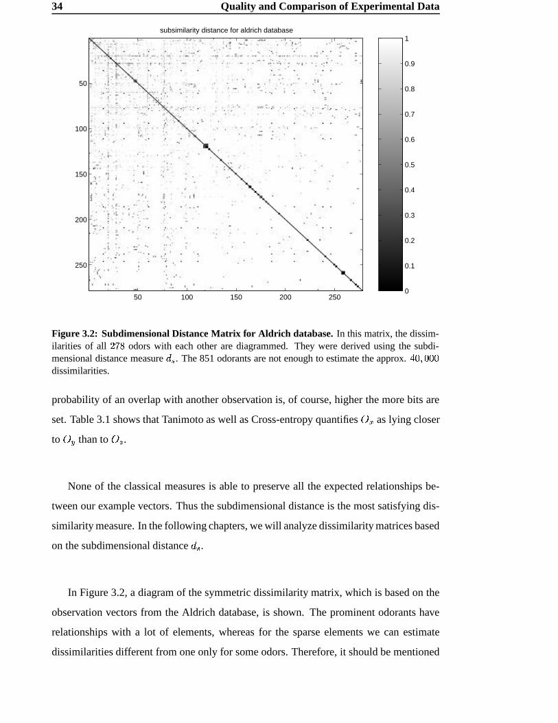
Figure 3.2: Subdimensional Distance Matrix for Aldrich database. In this matrix, the dissim-ilarities of all þ$ÿ�� odors with each other are diagrammed. They were derived using the subdi-mensional distance measure ø Ì . The 851 odorants are not enough to estimate the approx. �����������dissimilarities.
probability of an overlap with another observation is, of course, higher the more bits are
set. Table 3.1 shows that Tanimoto as well as Cross-entropy quantifies =U> as lying closer
to =?A than to =NX .None of the classical measures is able to preserve all the expected relationships be-
tween our example vectors. Thus the subdimensional distance is the most satisfying dis-
similarity measure. In the following chapters, we will analyze dissimilarity matrices based
on the subdimensional distance KcÌ .In Figure 3.2, a diagram of the symmetric dissimilarity matrix, which is based on the
observation vectors from the Aldrich database, is shown. The prominent odorants have
relationships with a lot of elements, whereas for the sparse elements we can estimate
dissimilarities different from one only for some odors. Therefore, it should be mentioned
3.4 Estimating dissimilarities in the Odor Space 35
that, unfortunately, a huge number of entries has got the maximal value of one. This
is because a lot of odors cannot be related to each other. We have only 851 odorants
to estimate about ÃR c"C � � dissimilarities. There might be unknown odorants that would
model the similarity between two odors better.
To our knowledge, the subdimensional distance measure KÇÌ expresses intuitively sat-
isfying relationships between odors. But, of course, it can just represent an estimate of
odor distance. We hope that our maps might increase the understanding of the existing re-
lationships between odors. The question “How to measure odor distances?” is still one of
the essential questions in analyzing odor perception; this problem should not be neglected
in future work.
C H A P T E R 4
Multidimensional Scaling
Given a set of � arbitrary points in a -dimensional Euclidean space, it is very easy to
construct a symmetric � �9� matrix containing all distances between all � points. Such a
matrix is called a distance matrix. These distances can be calculated using a metric e.g.
the Euclidean metric. An example is given in Figure 4.2 with its corresponding distance
matrix shown in Table 4.1. For more detailed information about metrics, please refer to
Chapter 3.
The inverted problem is much harder to solve. Given only a distance matrix, it is hard
to reconstruct the corresponding points. First of all, not even the correct dimensionality
can be derived directly out of the distance information. No matter what dimensionality the
original points have, distances are scalar values. Further, it is difficult to get a correct con-
figuration for all points, preserving the corresponding distances. The intuitive approach to
reconstructing the points would be to start with two points located at the correct distance.
Then, a third point can be added (as shown in figure 4.1) and so on. The problem is to
find the position for each point where the distances to all the other points are correct. Ad-
justing the distance between two points will affect the distances to all remaining points as
well. It should be mentioned that of course the orientation of the set of points cannot be
reconstructed. This is because only internal relationships are stored in a distance matrix,
not global orientation information.
Multidimensional Scaling (MDS) is an approach that leads to a numerical solution
4.1 Mathematical Model 37
3P
d13
P2
P1
3P’ d
d23
12
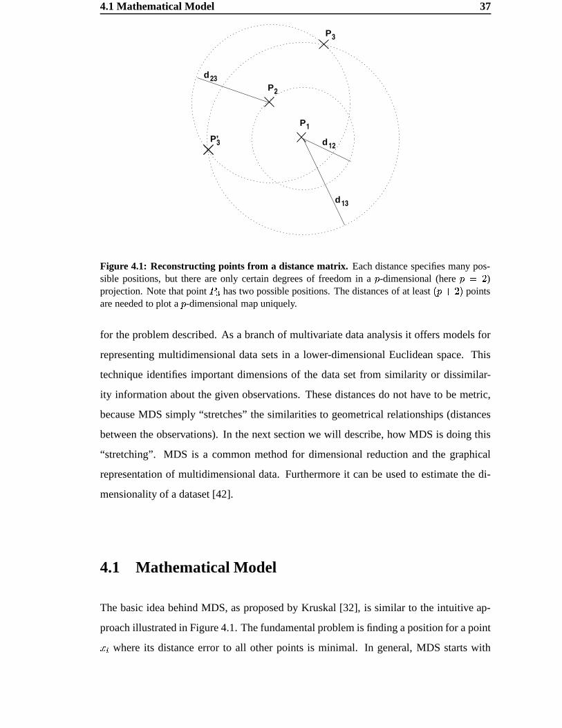
Figure 4.1: Reconstructing points from a distance matrix. Each distance specifies many pos-sible positions, but there are only certain degrees of freedom in a -dimensional (here � þ )projection. Note that point � � has two possible positions. The distances of at least ���þ�� pointsare needed to plot a -dimensional map uniquely.
for the problem described. As a branch of multivariate data analysis it offers models for
representing multidimensional data sets in a lower-dimensional Euclidean space. This
technique identifies important dimensions of the data set from similarity or dissimilar-
ity information about the given observations. These distances do not have to be metric,
because MDS simply “stretches” the similarities to geometrical relationships (distances
between the observations). In the next section we will describe, how MDS is doing this
“stretching”. MDS is a common method for dimensional reduction and the graphical
representation of multidimensional data. Furthermore it can be used to estimate the di-
mensionality of a dataset [42].
4.1 Mathematical Model
The basic idea behind MDS, as proposed by Kruskal [32], is similar to the intuitive ap-
proach illustrated in Figure 4.1. The fundamental problem is finding a position for a point* l where its distance error to all other points is minimal. In general, MDS starts with
38 Multidimensional Scaling
a randomized or normalized configuration for the � points * B "H�#�#�H"`* D . Repeatedly, all
points are pinned down one after the other and the distances to all the other points are
corrected. The scaling is finished after a given number of iterations or after a minimal
configuration has been reached. This happens if the distances cannot be corrected any
further.
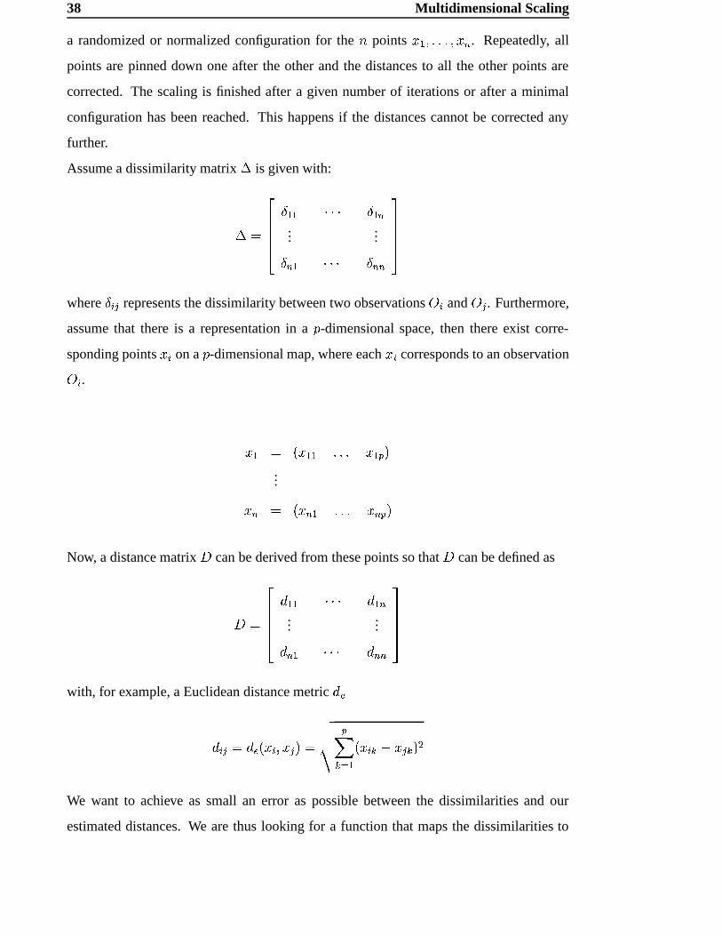
Assume a dissimilarity matrix � is given with:
� . ¡¢¢¢£�� BJB 7%7%7 � BÍD...
...� D+B 7%7%7 � DHD¤¦¥¥¥§
where � l © represents the dissimilarity between two observations = l and =�© . Furthermore,
assume that there is a representation in a -dimensional space, then there exist corre-
sponding points * l on a -dimensional map, where each * l corresponds to an observation= l .* B . �Í* BJB �#�#� * B�� �
...* D . �Í* D�B �#�H� * D�� �Now, a distance matrix � can be derived from these points so that � can be defined as
� . ¡¢¢¢£ K BJB 7%7%7 K BÍD...
...K D�B 7%7%7 K DHD¤¦¥¥¥§
with, for example, a Euclidean distance metric Kc~K l © . KR~H�Í* l "`*¿©H� . ���� �j � ¹ B �Í* l � �ö*¿© � � �
We want to achieve as small an error as possible between the dissimilarities and our
estimated distances. We are thus looking for a function that maps the dissimilarities to
4.1 Mathematical Model 39
distances, roughly speaking � Ï d Dj l¦¹ B �j © ¹ B ��� � � l ©�����K l ©I� �Kruskal [32] formulated a so-called stress function as
�! �"�#$�%� . � l � © ��� � � l ©�����K l ©I� �� l � © K �l ©The term “stress” should be interpreted as the strain of a spring whose end is joined
to the dissimilarity measure. The distance approximation pulls on the other end of the
spring. The stress is high if the displacement of the distance approximation to the dis-
similarity measure is large. The main difference between the several versions of MDS in
existence is the use of different scaling factors of the stress function [48].
4.1.1 An Example of Multidimensional Scaling
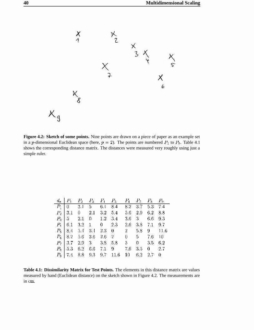
To illustrate the application of MDS a simple example – based on the sketch shown in Fig-
ure 4.2 – was scaled using MDS. The dissimilarity matrix is shown in Table 4.1. These
dissimilarities are just the distance between the points, measured roughly using a com-
mon ruler. Although they were derived using a metric, these dissimilarities will contain
certain errors. Even though this matrix describes only nine points, it is already difficult to
imagine the corresponding map without knowing the original. The map that results from
MDS (Figure 4.3) is almost identical to the sketch, apart from the fact that the map is
turned by a certain angle compared to the original. But this is not surprising – we cannot
expect to achieve the same orientation using MDS, due to the fact that no information
about orientation is stored in a distance matrix.
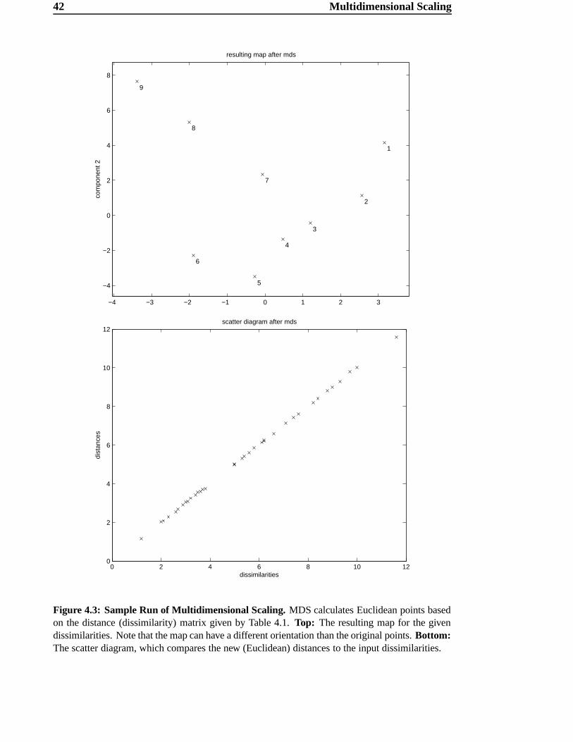
The so-called scatter plot is a common method for visualizing the quality of MDS
results [30]. This plot displays the quality of the approximation and the “stress” in the
mapping. A map is called “perfect” if the order of the dissimilarities is preserved in
40 Multidimensional Scaling
Figure 4.2: Sketch of some points. Nine points are drawn on a piece of paper as an example setin a -dimensional Euclidean space (here, &Qþ ). The points are numbered � B to �(' . Table 4.1shows the corresponding distance matrix. The distances were measured very roughly using just asimple ruler.
Ky~ / B / � / � / / ® / ¯ /*) /,+ / '/ B ¶��¾� � ���¾� ��÷à ��´� ¶���Ä �c�³¶ Äc�÷Ã/ � ¶��è� �c�¾� ¶���� �c�÷à �c��� �c�³) ����� ��³ / � � �c�¾� ����� ¶��÷à ¶���� ¶ ���³� )��³¶/ ���è� ¶���� � �c�³¶ �c��� ¶��³ Äc�¾� )���Ä/ ® ��³Ã �c�÷à ¶��÷à �c�³¶ � �c�³ ) �����³�/ ¯ ��´� �c�³� ¶��³� �c�³� � � Äc�³� �% /*) ¶��´Ä �c�³) ¶ ¶��³ �c�³ � ¶���� �����/,+ �c��¶ ����� ���³� Äc�¾� ) Äc��� ¶���� �c��Ä/ ' Äc�³Ã ��³ )��³¶ )���Ä ���!��� �% ����� �c��Ä Table 4.1: Dissimilarity Matrix for Test Points. The elements in this distance matrix are valuesmeasured by hand (Euclidean distance) on the sketch shown in Figure 4.2. The measurements arein -/. .
4.2 Estimating Dimensionality 41
the corresponding distance values, that is, the values in the scatter diagram have to grow
monotonously from left to right. Minimal “stress” would lead to a perfectly straight line
on the scatter plot. The scatter plot for our example can be seen in Figure 4.3. Of course,
usually MDS results are not so close to a straight line.
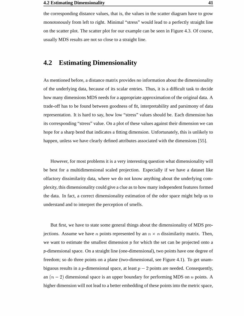
4.2 Estimating Dimensionality
As mentioned before, a distance matrix provides no information about the dimensionality
of the underlying data, because of its scalar entries. Thus, it is a difficult task to decide
how many dimensions MDS needs for a appropriate approximation of the original data. A
trade-off has to be found between goodness of fit, interpretability and parsimony of data
representation. It is hard to say, how low “stress” values should be. Each dimension has
its corresponding “stress” value. On a plot of these values against their dimension we can
hope for a sharp bend that indicates a fitting dimension. Unfortunately, this is unlikely to
happen, unless we have clearly defined attributes associated with the dimensions [55].
However, for most problems it is a very interesting question what dimensionality will
be best for a multidimensional scaled projection. Especially if we have a dataset like
olfactory dissimilarity data, where we do not know anything about the underlying com-
plexity, this dimensionality could give a clue as to how many independent features formed
the data. In fact, a correct dimensionality estimation of the odor space might help us to
understand and to interpret the perception of smells.
But first, we have to state some general things about the dimensionality of MDS pro-
jections. Assume we have � points represented by an �4� � dissimilarity matrix. Then,
we want to estimate the smallest dimension for which the set can be projected onto a -dimensional space. On a straight line (one-dimensional), two points have one degree of
freedom; so do three points on a plane (two-dimensional, see Figure 4.1). To get unam-
biguous results in a -dimensional space, at least ¸\ � points are needed. Consequently,
an ��� � ��� dimensional space is an upper boundary for performing MDS on � points. A
higher dimension will not lead to a better embedding of these points into the metric space,
42 Multidimensional Scaling
−4 −3 −2 −1 0 1 2 3
−4
−2
0
2
4
6
8
1
2
3
4
5
6
7
8
9
resulting map after mds
component 1
com
pone
nt 2
0 2 4 6 8 10 120
2
4
6
8
10
12scatter diagram after mds
dissimilarities
dist
ance
s
Figure 4.3: Sample Run of Multidimensional Scaling. MDS calculates Euclidean points basedon the distance (dissimilarity) matrix given by Table 4.1. Top: The resulting map for the givendissimilarities. Note that the map can have a different orientation than the original points. Bottom:The scatter diagram, which compares the new (Euclidean) distances to the input dissimilarities.
4.3 Application on Dissimilarity Data 43
since each point then simply receives its own dimension.
If the extrinsic dimension of these � points should in fact be higher than �M� � , this ei-
ther indicates that there is not enough information or that the dataset might be non-metric
as well as not very close related to metric characteristics. Of course, we can project �points into a space with a dimension higher than � �]� , but all dimensions beyond �:�ú�will lead to some kind of trivial solution. In other words, � points are just not able to span
more than �:� � dimensions.
However, we are interested in an estimation of the lower bound. What is the smallest
dimensionality that represents the dissimilarities with acceptable quality? In this thesis,
we use a simple method to estimate the lower bound roughly. Assuming we have a dis-
similarity matrix derived from � -dimensional points, then we will not be able to increase
the quality of a projection by increasing the dimension of the projection space beyond� . This is because the relationships between the points can be captured perfectly in � di-
mensions. Thus, the quality of an MDS projection will not increase significantly between
an � - and an �v\ � -dimensional MDS, once the appropriate dimensionality � has been
reached. Any dimension higher than this will be pointless for this data set.
4.3 Application on Dissimilarity Data
The same process was applied to the odor data set. Starting at a low dimension we ob-
served the projection quality of the MDS to get a rough estimate of the dimension at
which we seem to obtain the best results. Anyhow, the problem of the dimensionality of
odor space should be a topic of further research, especially with an eye to the extraction
of independent sets of odors.
To perform MDS on data related to odor perception, we used (as described in Chapter
3) a dataset based on the Aldrich Flavor and Fragrances Catalog [2]. To estimate dissim-
ilarities between different odors, the best results were obtained using the subdimensional
44 Multidimensional Scaling
Figure 4.4: Scatter Plot of two dimensional MDS on Aldrich database. Dissimilarities 0 l areplotted against the corresponding distance ø l after 2D MDS. The discrepancy between dissimilar-ities and the estimated distances is obvious.
distance K¿Ì (see Section 3.4.1). Again, it should be mentioned that “best” in the context
of distance estimation means that the chosen (semi-) metric yields the intuitively most
satisfying results for the dissimilarities of two observations =U> and =?A .4.3.1 A First Approach using 2D MDS
In a first attempt the odor data were projected directly onto a two-dimensional Euclidean
space. The main goal of this project was to derive a map for odors; thus, a two- or pos-
sibly three-dimensional projection would be exactly what we are looking for. On the
other hand, MDS applied the odor data with a two-dimensional target space is not a very
promising approach, because we expect the space to be high-dimensional and possibly
not even metric. For this reason, it is not very likely that we can find a satisfying configu-
ration in such a low dimensional Euclidean space.
The result of the two-dimensional projection of the Aldrich database is shown in Fig-
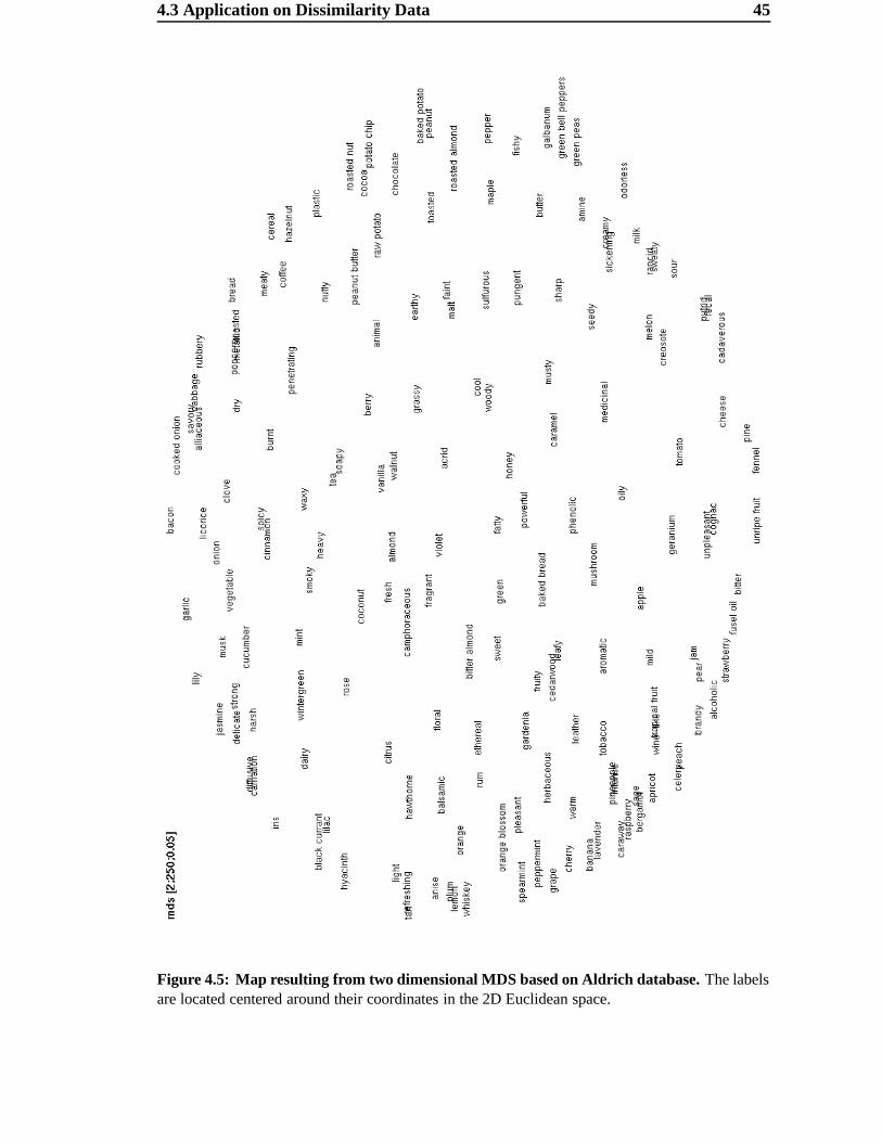
4.3 Application on Dissimilarity Data 45
Figure 4.5: Map resulting from two dimensional MDS based on Aldrich database. The labelsare located centered around their coordinates in the 2D Euclidean space.
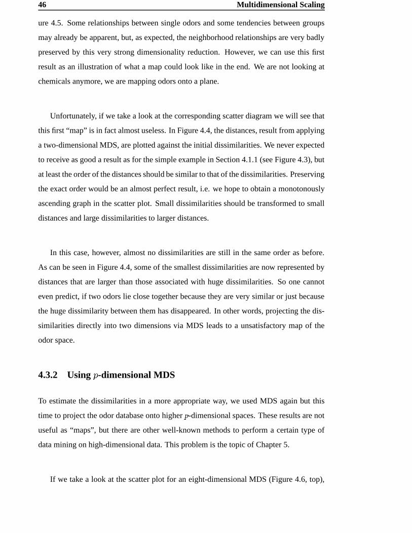
46 Multidimensional Scaling
ure 4.5. Some relationships between single odors and some tendencies between groups
may already be apparent, but, as expected, the neighborhood relationships are very badly
preserved by this very strong dimensionality reduction. However, we can use this first
result as an illustration of what a map could look like in the end. We are not looking at
chemicals anymore, we are mapping odors onto a plane.
Unfortunately, if we take a look at the corresponding scatter diagram we will see that
this first “map” is in fact almost useless. In Figure 4.4, the distances, result from applying
a two-dimensional MDS, are plotted against the initial dissimilarities. We never expected
to receive as good a result as for the simple example in Section 4.1.1 (see Figure 4.3), but
at least the order of the distances should be similar to that of the dissimilarities. Preserving
the exact order would be an almost perfect result, i.e. we hope to obtain a monotonously
ascending graph in the scatter plot. Small dissimilarities should be transformed to small
distances and large dissimilarities to larger distances.
In this case, however, almost no dissimilarities are still in the same order as before.
As can be seen in Figure 4.4, some of the smallest dissimilarities are now represented by
distances that are larger than those associated with huge dissimilarities. So one cannot
even predict, if two odors lie close together because they are very similar or just because
the huge dissimilarity between them has disappeared. In other words, projecting the dis-
similarities directly into two dimensions via MDS leads to a unsatisfactory map of the
odor space.
4.3.2 Using 1 -dimensional MDS
To estimate the dissimilarities in a more appropriate way, we used MDS again but this
time to project the odor database onto higher -dimensional spaces. These results are not
useful as “maps”, but there are other well-known methods to perform a certain type of
data mining on high-dimensional data. This problem is the topic of Chapter 5.
If we take a look at the scatter plot for an eight-dimensional MDS (Figure 4.6, top),
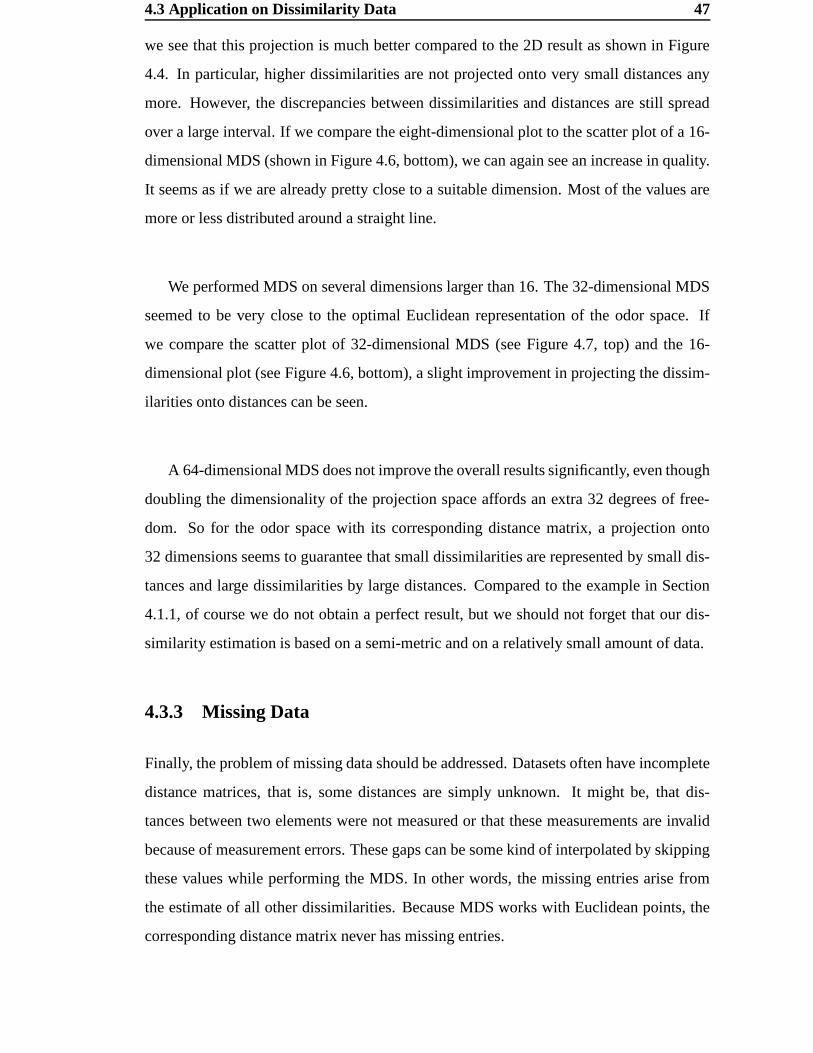
4.3 Application on Dissimilarity Data 47
we see that this projection is much better compared to the 2D result as shown in Figure
4.4. In particular, higher dissimilarities are not projected onto very small distances any
more. However, the discrepancies between dissimilarities and distances are still spread
over a large interval. If we compare the eight-dimensional plot to the scatter plot of a 16-
dimensional MDS (shown in Figure 4.6, bottom), we can again see an increase in quality.
It seems as if we are already pretty close to a suitable dimension. Most of the values are
more or less distributed around a straight line.
We performed MDS on several dimensions larger than 16. The 32-dimensional MDS
seemed to be very close to the optimal Euclidean representation of the odor space. If
we compare the scatter plot of 32-dimensional MDS (see Figure 4.7, top) and the 16-
dimensional plot (see Figure 4.6, bottom), a slight improvement in projecting the dissim-
ilarities onto distances can be seen.
A 64-dimensional MDS does not improve the overall results significantly, even though
doubling the dimensionality of the projection space affords an extra 32 degrees of free-
dom. So for the odor space with its corresponding distance matrix, a projection onto
32 dimensions seems to guarantee that small dissimilarities are represented by small dis-
tances and large dissimilarities by large distances. Compared to the example in Section
4.1.1, of course we do not obtain a perfect result, but we should not forget that our dis-
similarity estimation is based on a semi-metric and on a relatively small amount of data.
4.3.3 Missing Data
Finally, the problem of missing data should be addressed. Datasets often have incomplete
distance matrices, that is, some distances are simply unknown. It might be, that dis-
tances between two elements were not measured or that these measurements are invalid
because of measurement errors. These gaps can be some kind of interpolated by skipping
these values while performing the MDS. In other words, the missing entries arise from
the estimate of all other dissimilarities. Because MDS works with Euclidean points, the
corresponding distance matrix never has missing entries.
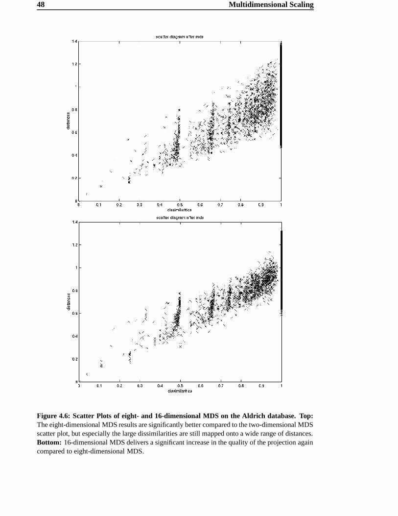
48 Multidimensional Scaling
Figure 4.6: Scatter Plots of eight- and 16-dimensional MDS on the Aldrich database. Top:The eight-dimensional MDS results are significantly better compared to the two-dimensional MDSscatter plot, but especially the large dissimilarities are still mapped onto a wide range of distances.Bottom: 16-dimensional MDS delivers a significant increase in the quality of the projection againcompared to eight-dimensional MDS.
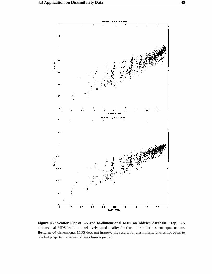
4.3 Application on Dissimilarity Data 49
Figure 4.7: Scatter Plot of 32- and 64-dimensional MDS on Aldrich database. Top: 32-dimensional MDS leads to a relatively good quality for those dissimilarities not equal to one.Bottom: 64-dimensional MDS does not improve the results for dissimilarity entries not equal toone but projects the values of one closer together.
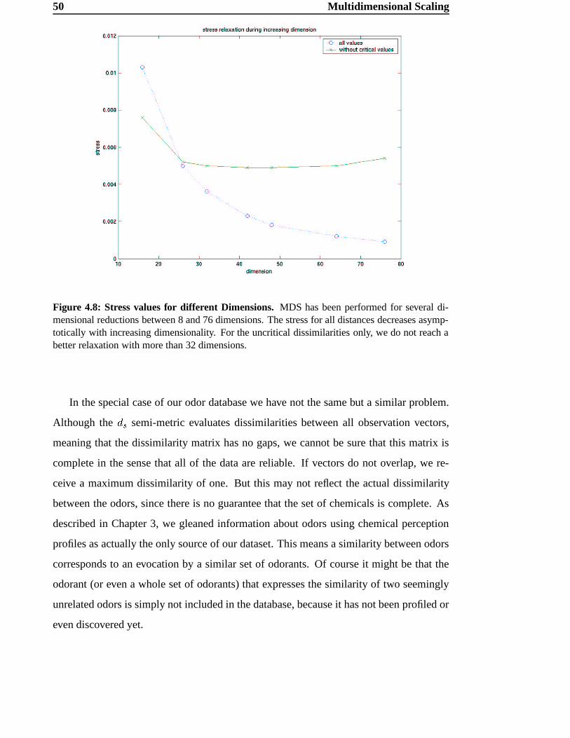
50 Multidimensional Scaling
Figure 4.8: Stress values for different Dimensions. MDS has been performed for several di-mensional reductions between 8 and 76 dimensions. The stress for all distances decreases asymp-totically with increasing dimensionality. For the uncritical dissimilarities only, we do not reach abetter relaxation with more than 32 dimensions.
In the special case of our odor database we have not the same but a similar problem.
Although the K¿Ì semi-metric evaluates dissimilarities between all observation vectors,
meaning that the dissimilarity matrix has no gaps, we cannot be sure that this matrix is
complete in the sense that all of the data are reliable. If vectors do not overlap, we re-
ceive a maximum dissimilarity of one. But this may not reflect the actual dissimilarity
between the odors, since there is no guarantee that the set of chemicals is complete. As
described in Chapter 3, we gleaned information about odors using chemical perception
profiles as actually the only source of our dataset. This means a similarity between odors
corresponds to an evocation by a similar set of odorants. Of course it might be that the
odorant (or even a whole set of odorants) that expresses the similarity of two seemingly
unrelated odors is simply not included in the database, because it has not been profiled or
even discovered yet.
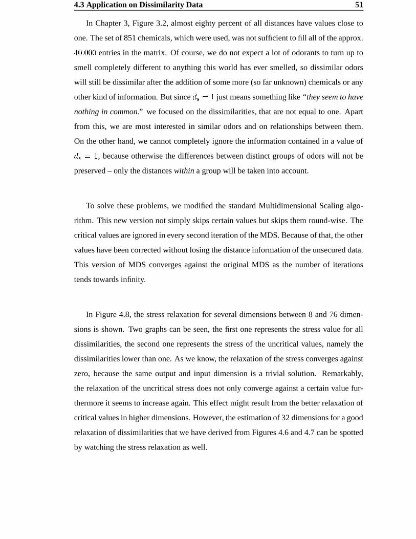
4.3 Application on Dissimilarity Data 51
In Chapter 3, Figure 3.2, almost eighty percent of all distances have values close to
one. The set of 851 chemicals, which were used, was not sufficient to fill all of the approx.ÃR ��³ � � entries in the matrix. Of course, we do not expect a lot of odorants to turn up to
smell completely different to anything this world has ever smelled, so dissimilar odors
will still be dissimilar after the addition of some more (so far unknown) chemicals or any
other kind of information. But since KcÌ . � just means something like “they seem to have
nothing in common.” we focused on the dissimilarities, that are not equal to one. Apart
from this, we are most interested in similar odors and on relationships between them.
On the other hand, we cannot completely ignore the information contained in a value ofK¿Ì . � , because otherwise the differences between distinct groups of odors will not be
preserved – only the distances within a group will be taken into account.
To solve these problems, we modified the standard Multidimensional Scaling algo-
rithm. This new version not simply skips certain values but skips them round-wise. The
critical values are ignored in every second iteration of the MDS. Because of that, the other
values have been corrected without losing the distance information of the unsecured data.
This version of MDS converges against the original MDS as the number of iterations
tends towards infinity.
In Figure 4.8, the stress relaxation for several dimensions between 8 and 76 dimen-
sions is shown. Two graphs can be seen, the first one represents the stress value for all
dissimilarities, the second one represents the stress of the uncritical values, namely the
dissimilarities lower than one. As we know, the relaxation of the stress converges against
zero, because the same output and input dimension is a trivial solution. Remarkably,
the relaxation of the uncritical stress does not only converge against a certain value fur-
thermore it seems to increase again. This effect might result from the better relaxation of
critical values in higher dimensions. However, the estimation of 32 dimensions for a good
relaxation of dissimilarities that we have derived from Figures 4.6 and 4.7 can be spotted
by watching the stress relaxation as well.
52 Multidimensional Scaling
4.3.4 Accuracy of Results
Two major problems occur if MDS is applied on odor dissimilarities. First, MDS might
reach as a numerical minimization method a local minimum instead of a global minimum.
Therefore, several runs should be performed with different starting configurations [55]. If
MDS still reaches a similar configuration, we can assume that we might have reached a
global and not only a local minimum.
In addition, we have to deal with the problem of missing data, as discussed in Section
4.3.3. It is far from clear whether MDS will end with several degrees of freedom or not.
Except for rotation, it is possible to get ambiguous configurations that solve the mapping
problem.
Hence, we performed a Monte-Carlo-simulation on our starting configurations. For
each dimensionality we run MDS 50 times, each time with a starting configuration that
was chosen by random. To compare the results, we calculated the standard deviation of
each inter-point distance ( � distances) and their corresponding confidence intervals.
We computed )R��� -confidence intervals (see Definition A.1.5) for the standard devi-
ations based on K -dimensional data, where K . �%��"C¶R�¿"IÃy� . For that purpose we used a
classical method assuming normally distributed data. This is justified here, because the
empirical kurtosis turned out to be rather small, less than one percent on average.
Since we did this calculation for all approx.73000 inter-point distances, the results
are not very easy to represent. The empirical standard deviations (see Definition A.1.3)
for the results of a 32-dimensional MDS have been sorted and downsampled. So, the
remaining deviations are representing the overall distribution of the standard deviation.
Interestingly, for most of the points we have a standard deviation of less than two percent.
These results are much better than expected, especially referring to the missing data prob-
lem.
In Figure 4.9 different dimensions are compared. To argue that a certain dimensional
4.3 Application on Dissimilarity Data 53
0 10 20 30 40 50 60 70 80 90 1000
0.01
0.02
0.03
0.04
0.05
0.06
0.07
downsampled standard deviation − comparison of 16, 32 and 42 dimensionsal MDS
16 dimensional stddev32 dimensional stddev42 dimensional stddev
Figure 4.9: Comparison of 16D, 32D and 42D MDS results on Aldrich database. The con-fidence intervals between 16D and 32D MDS are clearly disjunctive. The overlap seen between32D and 42D indicates, that we cannot be sure, whether we obtain better results or not. Here wetook 100 equally distributed representatives out of the ordered and complete set of approx. 73000inter-point distances.
representation is more sufficient than another, the confidence intervals of their corre-
sponding deviations should not overlap. In conformity with the presumption in Section
4.3.2, the 32-dimensional estimate yields significant better results compared to results
from 16-dimensional MDS. On the other hand, if we compare 32-dimensional MDS to
42-dimensional MDS, we observe an overlap of the confidence intervals.
Considering these results, it is reasonable to assume that there is a robust configuration
for MDS derived from the odor dissimilarity matrix. Beyond this, there is evidence that
a good approximation of the odor space – based on this data – can be made with an
Euclidean space of approx. 32 dimensions. Thus, a 32-dimensional representation of
odor space will be used as a data source in the next chapters.
C H A P T E R 5
Self Organizing Maps
In the previous chapters, we used a special metric – the so-called subdimensional distanceK¿Ì , as introduced in Section 3.4.1 – to estimate dissimilarities in psychophysical odor data.
Then, in Chapter 4, we used a multidimensional scaling method to project the odor space
model onto a Euclidean space. Unfortunately, this space seems to be very complex, so we
had to use an approximately 32-dimensional Euclidean space to preserve as many inter-
point relationships as possible. In this chapter, the emphasis will be on the visualization
and analysis of the preprocessed data, i.e. the 32-dimensional Euclidean representation of
odor dissimilarity data.
It may be useful to note that the preprocessing has a much higher impact on the re-
sult than the choice of the analysis method. However, the scope of this chapter is to
make the data more readable by projecting as many relationships as possible onto a two-
dimensional map.
There are two general approaches to handling multidimensional data sets. First, we
can search for groups of elements that have a close relationship to each other. Such groups
are called clusters. The search for such groups is called clustering. Clustered data can
be used to examine neighborhood relationships or to search for features that might be
characteristic for certain clusters. The second approach is to reduce the dimensionality of
the system in such a way that a human-readable map (meaning a two- or at most three-
dimensional map) is produced for visualization of the dataset. Based on such a map,
5.1 Visualization of high-dimensional data 55
further examinations can be performed by a human.
In Chapter 4, the odor space seemed to be much too complex to obtain a high quality
representation in only two dimensions. Thus, we have to find a combination of clustering
and visualization methods. Neural network algorithms have already been used for a wide
variety of applications, for visualization problems as well as for data analysis. Kohonen
[29] gives a comprehensive treatment of this subject. We will use so-called self-organizing
maps (SOMs or Kohonen maps) as a tool to visualize and to analyze the multidimensional
odor space that we have obtained by MDS in Chapter 4.
5.1 Visualization of high-dimensional data
An intuitive approach to visualizing high-dimensional data is to use a “profile” of the
feature vectors. This profile might be simply a graphical representation of the entries of
the features. The same, two prominent dimensions (the first two principal components,
for example) can be used as a two-dimensional location for the feature vector, while the
remaining features are used as icon properties (colors, shape, polygons etc.).
The drawback of such methods is clearly that they do not reduce the amount of data.
Analyzing a large data set will not become much easier than examining the raw data.
On the other hand, if relevant features are known already, these methods can be useful
to emphasize such characteristics. Faces are a classical example for the use of icons for
visualization. Features like eye distance, size of the mouth and skin color can be expressed
through a face icon that characterizes a face much more intuitively than a vector could do
[6]. Jain [25] introduces some more examples for the handling of known features.
5.2 Self-Organizing Maps (SOMs)
A self-organizing map (SOM) is a set of artificial neurons that is organized as a regular
low-dimensional grid. We use these maps to express a high-dimensional input space 2
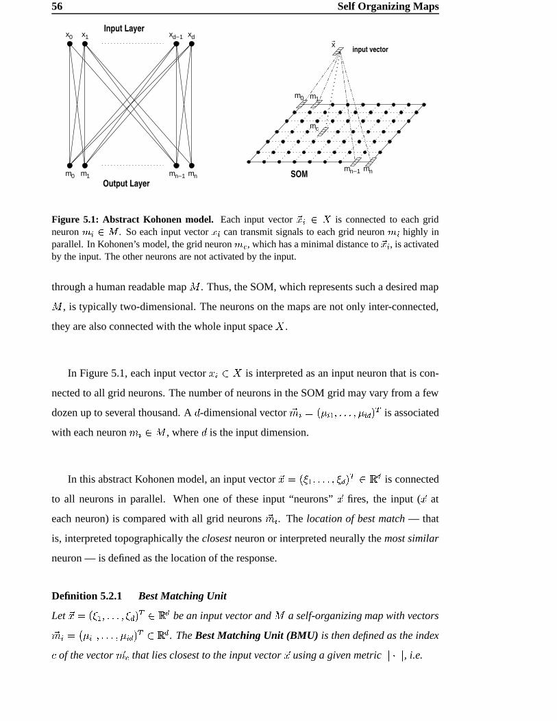
56 Self Organizing Maps
mnmn−1
m0 m1
x1x0 d−1x xd
m0 m1 mn−1 mn
x
Output Layer
Input Layer
SOM
input vector
mc
Figure 5.1: Abstract Kohonen model. Each input vector 34 l6587is connected to each grid
neuron 9 l 5;: . So each input vector 4 l can transmit signals to each grid neuron 9 l highly inparallel. In Kohonen’s model, the grid neuron 9 x , which has a minimal distance to 34 l , is activatedby the input. The other neurons are not activated by the input.
through a human readable map < . Thus, the SOM, which represents such a desired map< , is typically two-dimensional. The neurons on the maps are not only inter-connected,
they are also connected with the whole input space 2 .
In Figure 5.1, each input vector * l u=2 is interpreted as an input neuron that is con-
nected to all grid neurons. The number of neurons in the SOM grid may vary from a few
dozen up to several thousand. A K -dimensional vector >? l . �A@ l B "#�#�H�H"�@ l ÎY� E is associated
with each neuron ? l u;< , where K is the input dimension.
In this abstract Kohonen model, an input vector >* . �CB B "#�H�#�H"DBHÎz� E u w Î is connected
to all neurons in parallel. When one of these input “neurons” >* fires, the input ( >* at
each neuron) is compared with all grid neurons >? l . The location of best match — that
is, interpreted topographically the closest neuron or interpreted neurally the most similar
neuron — is defined as the location of the response.
Definition 5.2.1 Best Matching Unit
Let >* . �CB B "#�#�#��"DB#Îz� E u9w Î be an input vector and < a self-organizing map with vectors>? l . �A@ l B "#�#�H�H"�@ l Îz� E u w Î . The Best Matching Unit (BMU) is then defined as the indexE of the vector >? x that lies closest to the input vector >* using a given metric 3ä3$7c3ä3 , i.e.
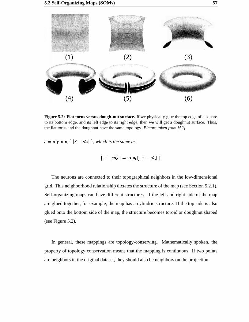
5.2 Self-Organizing Maps (SOMs) 57
Figure 5.2: Flat torus versus dough-nut surface. If we physically glue the top edge of a squareto its bottom edge, and its left edge to its right edge, then we will get a doughnut surface. Thus,the flat torus and the doughnut have the same topology. Picture taken from [52]E . ÐGF f �eÏ d l |É3ä3A>* �H>? l 3ä3�} , which is the same as3è3A>*e� >? x#3ä3 . �eÏ d l |É3è3A>*e�I>? l 3è3�}
The neurons are connected to their topographical neighbors in the low-dimensional
grid. This neighborhood relationship dictates the structure of the map (see Section 5.2.1).
Self-organizing maps can have different structures. If the left and right side of the map
are glued together, for example, the map has a cylindric structure. If the top side is also
glued onto the bottom side of the map, the structure becomes toroid or doughnut shaped
(see Figure 5.2).
In general, these mappings are topology-conserving. Mathematically spoken, the
property of topology conservation means that the mapping is continuous. If two points
are neighbors in the original dataset, they should also be neighbors on the projection.
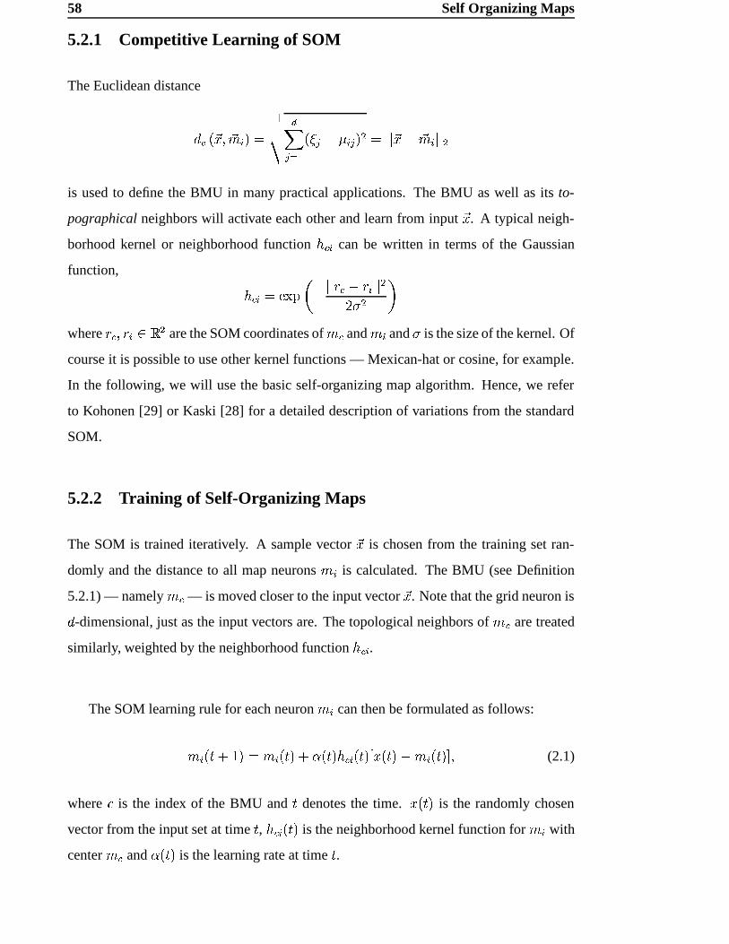
58 Self Organizing Maps
5.2.1 Competitive Learning of SOM
The Euclidean distance
KR~���>*8"J>? l � . ���� Îj © ¹ B �CBC©ý�K@ l ©z� � . 3è3A>*e�H>? l 3ä3 �is used to define the BMU in many practical applications. The BMU as well as its to-
pographical neighbors will activate each other and learn from input >* . A typical neigh-
borhood kernel or neighborhood function LLx l can be written in terms of the Gaussian
function, LÇx l . æ Ò$MON�� 3ä3 {Hx��ö{ l 3ä3 ��QP � Rwhere {#xI"I{ l uvw � are the SOM coordinates of ? x and ? l and P is the size of the kernel. Of
course it is possible to use other kernel functions — Mexican-hat or cosine, for example.
In the following, we will use the basic self-organizing map algorithm. Hence, we refer
to Kohonen [29] or Kaski [28] for a detailed description of variations from the standard
SOM.
5.2.2 Training of Self-Organizing Maps
The SOM is trained iteratively. A sample vector >* is chosen from the training set ran-
domly and the distance to all map neurons ? l is calculated. The BMU (see Definition
5.2.1) — namely ? x — is moved closer to the input vector >* . Note that the grid neuron isK -dimensional, just as the input vectors are. The topological neighbors of ? x are treated
similarly, weighted by the neighborhood function L,x l .The SOM learning rule for each neuron ? l can then be formulated as follows:
? l �CS�\Å�$� . ? l �CS`��\]�P�CS`�TLÇx l �CS`���6*��US`��� ? l �CS`�J�Ô" (2.1)
where E is the index of the BMU and S denotes the time. *��US`� is the randomly chosen
vector from the input set at time S , L�x l �CS`� is the neighborhood kernel function for ? l with
center ? x and �[�CS`� is the learning rate at time S .
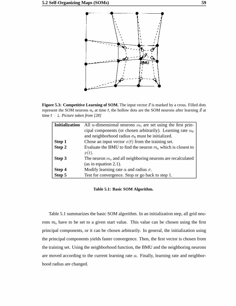
5.2 Self-Organizing Maps (SOMs) 59
Figure 5.3: Competitive Learning of SOM. The input vector 34 is marked by a cross. Filled dotsrepresent the SOM neurons ù l at time V , the hollow dots are the SOM neurons after learning 34 attime VW�KX . Picture taken from [28]
Initialization All � -dimensional neurons ? l are set using the first prin-cipal components (or chosen arbitrarily). Learning rate �ZYand neighborhood radius P[Y must be initialized.
Step 1 Chose an input vector *��US`� from the training set.Step 2 Evaluate the BMU to find the neuron ? x which is closest to*��CS`� .Step 3 The neuron ? x and all neighboring neurons are recalculated
(as in equation 2.1).Step 4 Modify learning rate � and radius P .Step 5 Test for convergence. Stop or go back to step 1.
Table 5.1: Basic SOM Algorithm.
Table 5.1 summarizes the basic SOM algorithm. In an initialization step, all grid neu-
rons ? l have to be set to a given start value. This value can be chosen using the first
principal components, or it can be chosen arbitrarily. In general, the initialization using
the principal components yields faster convergence. Then, the first vector is chosen from
the training set. Using the neighborhood function, the BMU and the neighboring neurons
are moved according to the current learning rate � . Finally, learning rate and neighbor-
hood radius are changed.
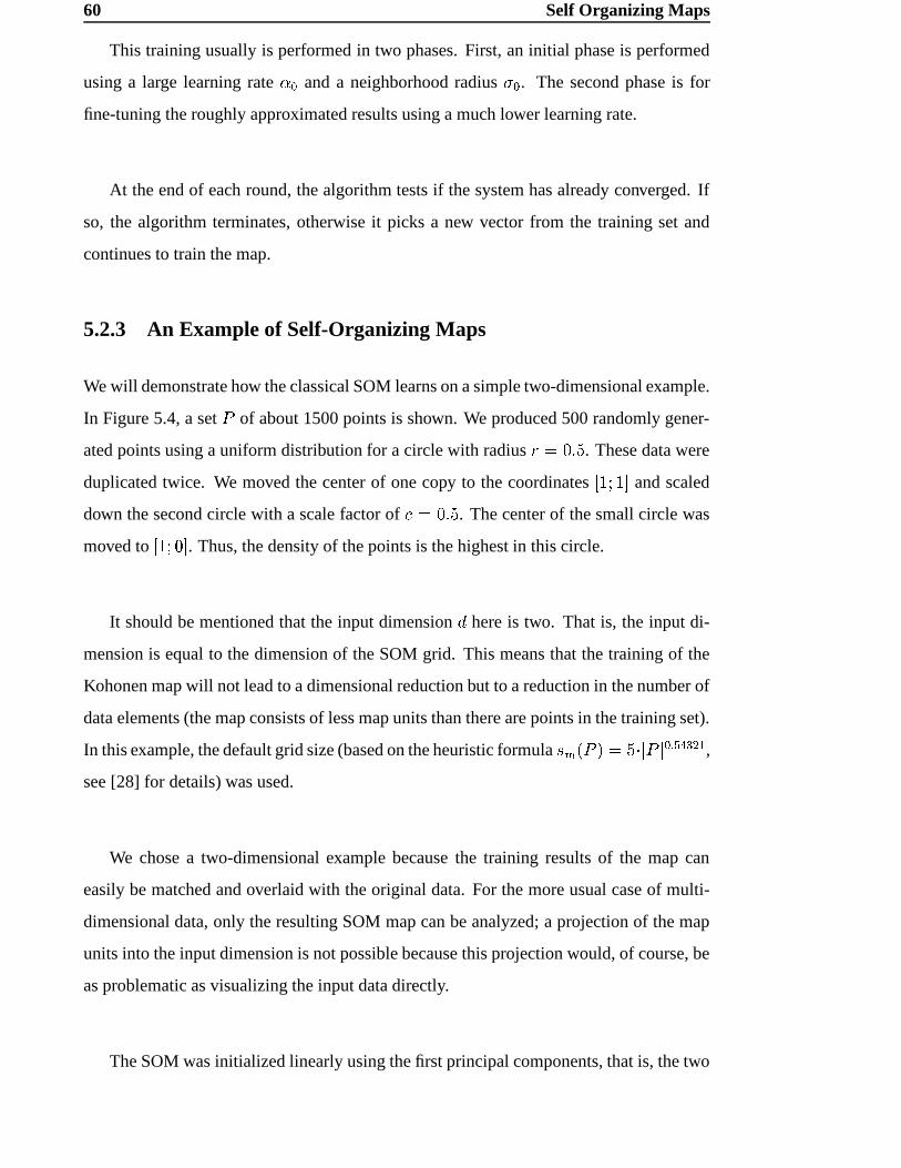
60 Self Organizing Maps
This training usually is performed in two phases. First, an initial phase is performed
using a large learning rate �,Y and a neighborhood radius P\Y . The second phase is for
fine-tuning the roughly approximated results using a much lower learning rate.
At the end of each round, the algorithm tests if the system has already converged. If
so, the algorithm terminates, otherwise it picks a new vector from the training set and
continues to train the map.
5.2.3 An Example of Self-Organizing Maps
We will demonstrate how the classical SOM learns on a simple two-dimensional example.
In Figure 5.4, a set / of about 1500 points is shown. We produced 500 randomly gener-
ated points using a uniform distribution for a circle with radius { . c�´� . These data were
duplicated twice. We moved the center of one copy to the coordinates �¦���#�H� and scaled
down the second circle with a scale factor of E . ���� . The center of the small circle was
moved to �¦���C �� . Thus, the density of the points is the highest in this circle.
It should be mentioned that the input dimension K here is two. That is, the input di-
mension is equal to the dimension of the SOM grid. This means that the training of the
Kohonen map will not lead to a dimensional reduction but to a reduction in the number of
data elements (the map consists of less map units than there are points in the training set).
In this example, the default grid size (based on the heuristic formula Ê+mN� / � . �Ç7F3 / 3 Y � ®Fü� � B ,see [28] for details) was used.
We chose a two-dimensional example because the training results of the map can
easily be matched and overlaid with the original data. For the more usual case of multi-
dimensional data, only the resulting SOM map can be analyzed; a projection of the map
units into the input dimension is not possible because this projection would, of course, be
as problematic as visualizing the input data directly.
The SOM was initialized linearly using the first principal components, that is, the two
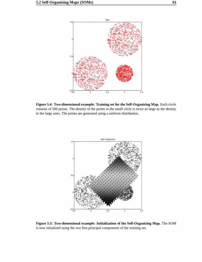
5.2 Self-Organizing Maps (SOMs) 61
−0.5 0 0.5 1 1.5−0.5
0
0.5
1
1.5Data
Figure 5.4: Two-dimensional example: Training set for the Self-Organizing Map. Each circleconsists of 500 points. The density of the points in the small circle is twice as large as the densityin the large ones. The points are generated using a uniform distribution.
−0.5 0 0.5 1 1.5−0.5
0
0.5
1
1.5After initialization
Figure 5.5: Two-dimensional example: Initialization of the Self-Organizing Map. The SOMis now initialized using the two first principal components of the training set.
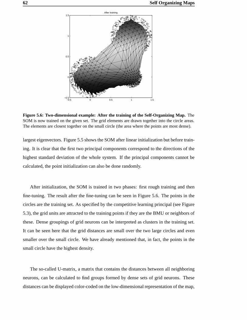
62 Self Organizing Maps
−0.5 0 0.5 1 1.5−0.5
0
0.5
1
1.5After training
Figure 5.6: Two-dimensional example: After the training of the Self-Organizing Map. TheSOM is now trained on the given set. The grid elements are drawn together into the circle areas.The elements are closest together on the small circle (the area where the points are most dense).
largest eigenvectors. Figure 5.5 shows the SOM after linear initialization but before train-
ing. It is clear that the first two principal components correspond to the directions of the
highest standard deviation of the whole system. If the principal components cannot be
calculated, the point initialization can also be done randomly.
After initialization, the SOM is trained in two phases: first rough training and then
fine-tuning. The result after the fine-tuning can be seen in Figure 5.6. The points in the
circles are the training set. As specified by the competitive learning principal (see Figure
5.3), the grid units are attracted to the training points if they are the BMU or neighbors of
these. Dense groupings of grid neurons can be interpreted as clusters in the training set.
It can be seen here that the grid distances are small over the two large circles and even
smaller over the small circle. We have already mentioned that, in fact, the points in the
small circle have the highest density.
The so-called U-matrix, a matrix that contains the distances between all neighboring
neurons, can be calculated to find groups formed by dense sets of grid neurons. These
distances can be displayed color-coded on the low-dimensional representation of the map,
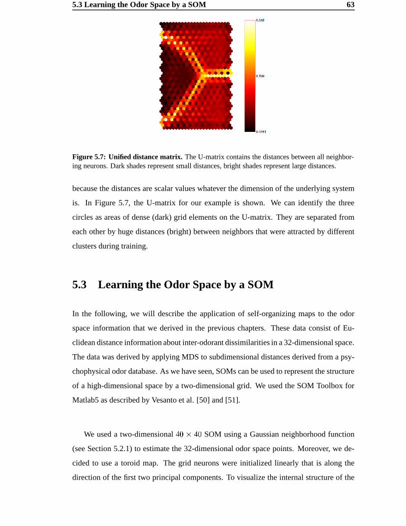
5.3 Learning the Odor Space by a SOM 63
Figure 5.7: Unified distance matrix. The U-matrix contains the distances between all neighbor-ing neurons. Dark shades represent small distances, bright shades represent large distances.
because the distances are scalar values whatever the dimension of the underlying system
is. In Figure 5.7, the U-matrix for our example is shown. We can identify the three
circles as areas of dense (dark) grid elements on the U-matrix. They are separated from
each other by huge distances (bright) between neighbors that were attracted by different
clusters during training.
5.3 Learning the Odor Space by a SOM
In the following, we will describe the application of self-organizing maps to the odor
space information that we derived in the previous chapters. These data consist of Eu-
clidean distance information about inter-odorant dissimilarities in a 32-dimensional space.
The data was derived by applying MDS to subdimensional distances derived from a psy-
chophysical odor database. As we have seen, SOMs can be used to represent the structure
of a high-dimensional space by a two-dimensional grid. We used the SOM Toolbox for
Matlab5 as described by Vesanto et al. [50] and [51].
We used a two-dimensional Ã� �öÃ� SOM using a Gaussian neighborhood function
(see Section 5.2.1) to estimate the 32-dimensional odor space points. Moreover, we de-
cided to use a toroid map. The grid neurons were initialized linearly that is along the
direction of the first two principal components. To visualize the internal structure of the
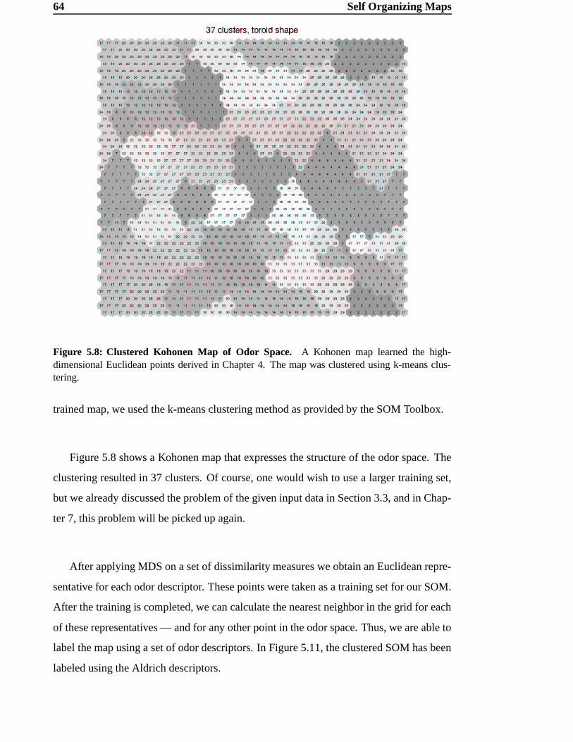
64 Self Organizing Maps
Figure 5.8: Clustered Kohonen Map of Odor Space. A Kohonen map learned the high-dimensional Euclidean points derived in Chapter 4. The map was clustered using k-means clus-tering.
trained map, we used the k-means clustering method as provided by the SOM Toolbox.
Figure 5.8 shows a Kohonen map that expresses the structure of the odor space. The
clustering resulted in 37 clusters. Of course, one would wish to use a larger training set,
but we already discussed the problem of the given input data in Section 3.3, and in Chap-
ter 7, this problem will be picked up again.
After applying MDS on a set of dissimilarity measures we obtain an Euclidean repre-
sentative for each odor descriptor. These points were taken as a training set for our SOM.
After the training is completed, we can calculate the nearest neighbor in the grid for each
of these representatives — and for any other point in the odor space. Thus, we are able to
label the map using a set of odor descriptors. In Figure 5.11, the clustered SOM has been
labeled using the Aldrich descriptors.
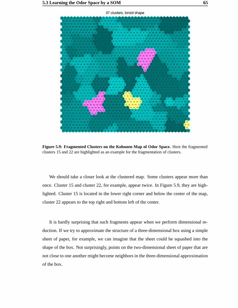
5.3 Learning the Odor Space by a SOM 65
Figure 5.9: Fragmented Clusters on the Kohonen Map of Odor Space. Here the fragmentedclusters 15 and 22 are highlighted as an example for the fragmentation of clusters.
We should take a closer look at the clustered map. Some clusters appear more than
once. Cluster 15 and cluster 22, for example, appear twice. In Figure 5.9, they are high-
lighted. Cluster 15 is located in the lower right corner and below the center of the map,
cluster 22 appears to the top right and bottom left of the center.
It is hardly surprising that such fragments appear when we perform dimensional re-
duction. If we try to approximate the structure of a three-dimensional box using a simple
sheet of paper, for example, we can imagine that the sheet could be squashed into the
shape of the box. Not surprisingly, points on the two-dimensional sheet of paper that are
not close to one another might become neighbors in the three-dimensional approximation
of the box.
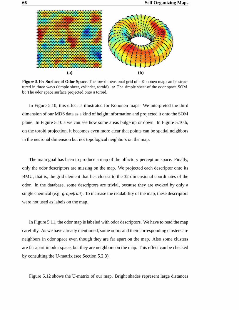
66 Self Organizing Maps
(a) (b)
Figure 5.10: Surface of Odor Space. The low-dimensional grid of a Kohonen map can be struc-tured in three ways (simple sheet, cylinder, toroid). a: The simple sheet of the odor space SOM.b: The odor space surface projected onto a toroid.
In Figure 5.10, this effect is illustrated for Kohonen maps. We interpreted the third
dimension of our MDS data as a kind of height information and projected it onto the SOM
plane. In Figure 5.10.a we can see how some areas bulge up or down. In Figure 5.10.b,
on the toroid projection, it becomes even more clear that points can be spatial neighbors
in the neuronal dimension but not topological neighbors on the map.
The main goal has been to produce a map of the olfactory perception space. Finally,
only the odor descriptors are missing on the map. We projected each descriptor onto its
BMU, that is, the grid element that lies closest to the 32-dimensional coordinates of the
odor. In the database, some descriptors are trivial, because they are evoked by only a
single chemical (e.g. grapefruit). To increase the readability of the map, these descriptors
were not used as labels on the map.
In Figure 5.11, the odor map is labeled with odor descriptors. We have to read the map
carefully. As we have already mentioned, some odors and their corresponding clusters are
neighbors in odor space even though they are far apart on the map. Also some clusters
are far apart in odor space, but they are neighbors on the map. This effect can be checked
by consulting the U-matrix (see Section 5.2.3).
Figure 5.12 shows the U-matrix of our map. Bright shades represent large distances
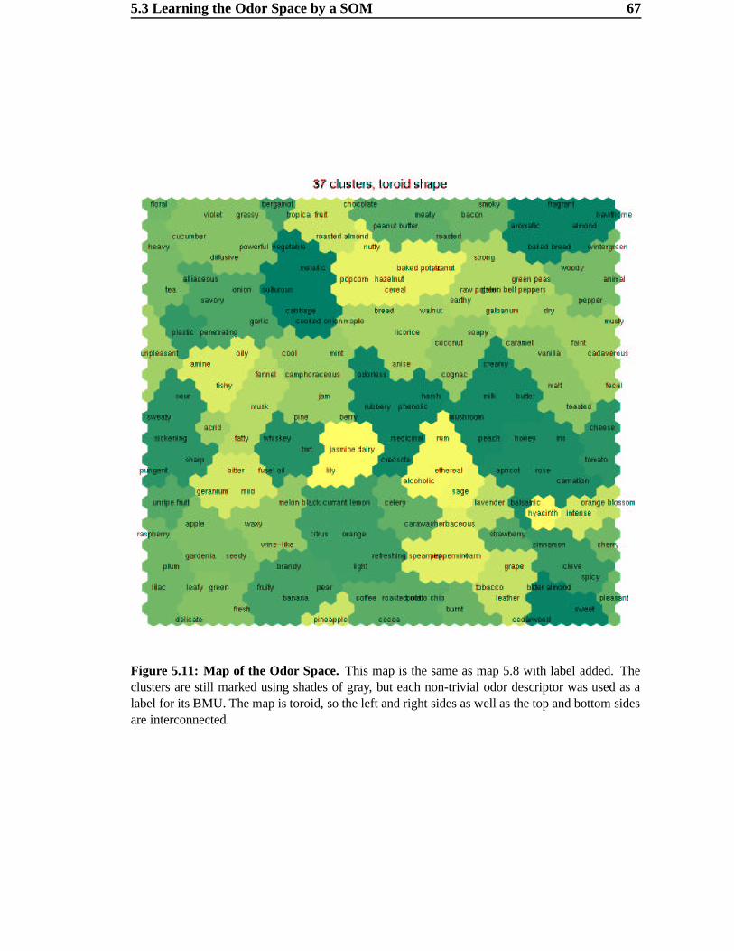
5.3 Learning the Odor Space by a SOM 67
Figure 5.11: Map of the Odor Space. This map is the same as map 5.8 with label added. Theclusters are still marked using shades of gray, but each non-trivial odor descriptor was used as alabel for its BMU. The map is toroid, so the left and right sides as well as the top and bottom sidesare interconnected.
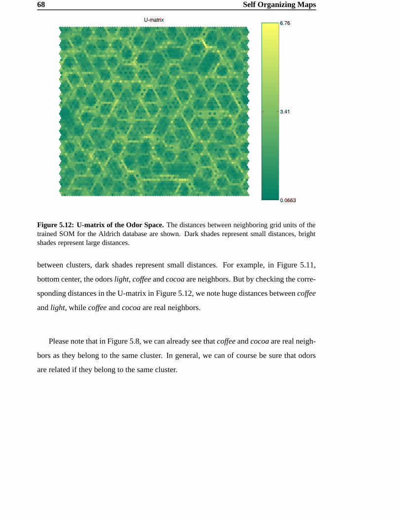
68 Self Organizing Maps
Figure 5.12: U-matrix of the Odor Space. The distances between neighboring grid units of thetrained SOM for the Aldrich database are shown. Dark shades represent small distances, brightshades represent large distances.
between clusters, dark shades represent small distances. For example, in Figure 5.11,
bottom center, the odors light, coffee and cocoa are neighbors. But by checking the corre-
sponding distances in the U-matrix in Figure 5.12, we note huge distances between coffee
and light, while coffee and cocoa are real neighbors.
Please note that in Figure 5.8, we can already see that coffee and cocoa are real neigh-
bors as they belong to the same cluster. In general, we can of course be sure that odors
are related if they belong to the same cluster.
C H A P T E R 6
Applications of the Olfactory Perception Map
In the previous chapters, we spent much time describing details, problems and restrictions
of our mapping infrastructure. The crucial question of the applicability of the map has
not been covered so far. Hence, in this chapter we will try to illustrate possibilities that
are enabled by this new approach. The mapping approach will be compared against the
old approach, the directed graph model of Chee-Ruiter [12].
We will conclude with fascinating evidence that we found for a hypothesis about ecolog-
ical proximities between chemicals.
6.1 The order of apple, banana and cherry
Even though it is known that Parkinson’s disease, for example, influences the sense of
smell, there are only a few simple tests available for the clinical use [15]. It can just be
tested whether or not a patient can detect a certain stimulus or not.
Our new approach has an outstanding property that is not in the scope of the models
proposed so far. We are able to quantify the order of odors. Some quantifications are not
very surprising. In Chapter 5, we motivated the use of the U-matrix with the question
whether coffee is more related to cocoa or to light. The insight that coffee is more closely
related to cocoa than to light is not very surprising.
But let us take another example. A popular example for the main problem in odor
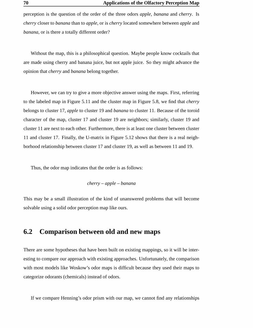
70 Applications of the Olfactory Perception Map
perception is the question of the order of the three odors apple, banana and cherry. Is
cherry closer to banana than to apple, or is cherry located somewhere between apple and
banana, or is there a totally different order?
Without the map, this is a philosophical question. Maybe people know cocktails that
are made using cherry and banana juice, but not apple juice. So they might advance the
opinion that cherry and banana belong together.
However, we can try to give a more objective answer using the maps. First, referring
to the labeled map in Figure 5.11 and the cluster map in Figure 5.8, we find that cherry
belongs to cluster 17, apple to cluster 19 and banana to cluster 11. Because of the toroid
character of the map, cluster 17 and cluster 19 are neighbors; similarly, cluster 19 and
cluster 11 are next to each other. Furthermore, there is at least one cluster between cluster
11 and cluster 17. Finally, the U-matrix in Figure 5.12 shows that there is a real neigh-
borhood relationship between cluster 17 and cluster 19, as well as between 11 and 19.
Thus, the odor map indicates that the order is as follows:
cherry – apple – banana
This may be a small illustration of the kind of unanswered problems that will become
solvable using a solid odor perception map like ours.
6.2 Comparison between old and new maps
There are some hypotheses that have been built on existing mappings, so it will be inter-
esting to compare our approach with existing approaches. Unfortunately, the comparison
with most models like Woskow’s odor maps is difficult because they used their maps to
categorize odorants (chemicals) instead of odors.
If we compare Henning’s odor prism with our map, we cannot find any relationships
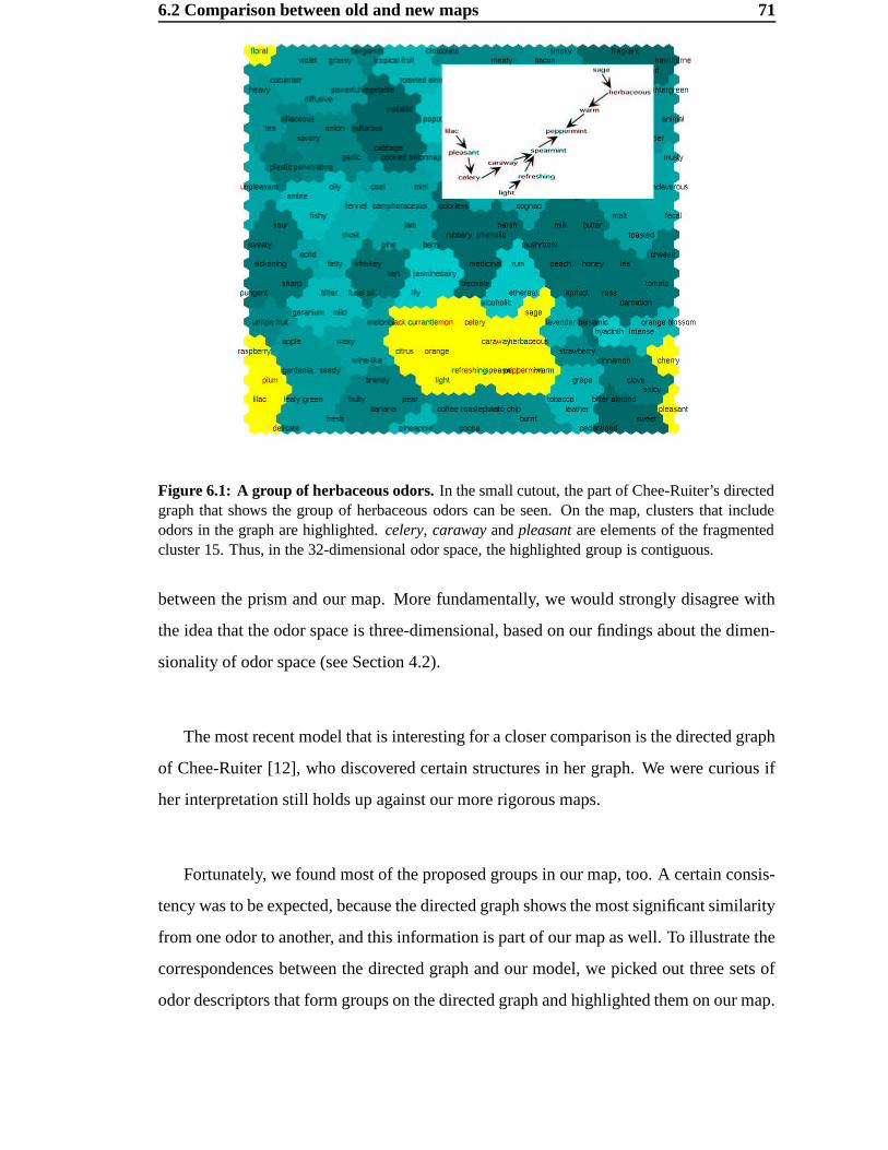
6.2 Comparison between old and new maps 71
Figure 6.1: A group of herbaceous odors. In the small cutout, the part of Chee-Ruiter’s directedgraph that shows the group of herbaceous odors can be seen. On the map, clusters that includeodors in the graph are highlighted. celery, caraway and pleasant are elements of the fragmentedcluster 15. Thus, in the 32-dimensional odor space, the highlighted group is contiguous.
between the prism and our map. More fundamentally, we would strongly disagree with
the idea that the odor space is three-dimensional, based on our findings about the dimen-
sionality of odor space (see Section 4.2).
The most recent model that is interesting for a closer comparison is the directed graph
of Chee-Ruiter [12], who discovered certain structures in her graph. We were curious if
her interpretation still holds up against our more rigorous maps.
Fortunately, we found most of the proposed groups in our map, too. A certain consis-
tency was to be expected, because the directed graph shows the most significant similarity
from one odor to another, and this information is part of our map as well. To illustrate the
correspondences between the directed graph and our model, we picked out three sets of
odor descriptors that form groups on the directed graph and highlighted them on our map.
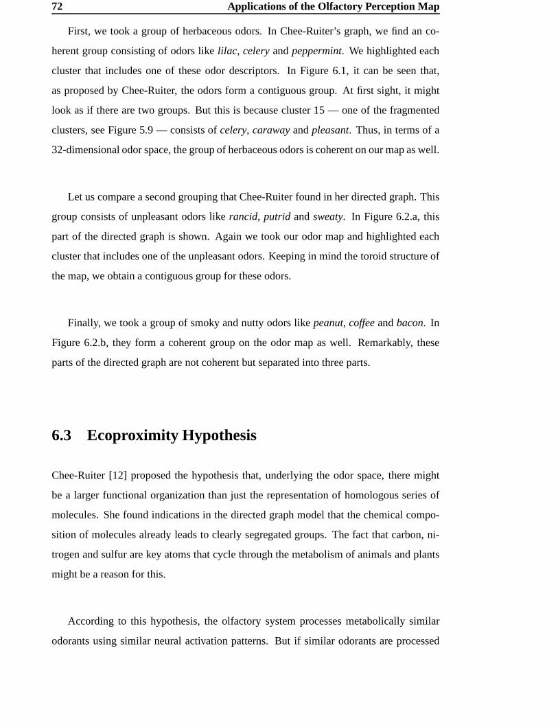
72 Applications of the Olfactory Perception Map
First, we took a group of herbaceous odors. In Chee-Ruiter’s graph, we find an co-
herent group consisting of odors like lilac, celery and peppermint. We highlighted each
cluster that includes one of these odor descriptors. In Figure 6.1, it can be seen that,
as proposed by Chee-Ruiter, the odors form a contiguous group. At first sight, it might
look as if there are two groups. But this is because cluster 15 — one of the fragmented
clusters, see Figure 5.9 — consists of celery, caraway and pleasant. Thus, in terms of a
32-dimensional odor space, the group of herbaceous odors is coherent on our map as well.
Let us compare a second grouping that Chee-Ruiter found in her directed graph. This
group consists of unpleasant odors like rancid, putrid and sweaty. In Figure 6.2.a, this
part of the directed graph is shown. Again we took our odor map and highlighted each
cluster that includes one of the unpleasant odors. Keeping in mind the toroid structure of
the map, we obtain a contiguous group for these odors.
Finally, we took a group of smoky and nutty odors like peanut, coffee and bacon. In
Figure 6.2.b, they form a coherent group on the odor map as well. Remarkably, these
parts of the directed graph are not coherent but separated into three parts.
6.3 Ecoproximity Hypothesis
Chee-Ruiter [12] proposed the hypothesis that, underlying the odor space, there might
be a larger functional organization than just the representation of homologous series of
molecules. She found indications in the directed graph model that the chemical compo-
sition of molecules already leads to clearly segregated groups. The fact that carbon, ni-
trogen and sulfur are key atoms that cycle through the metabolism of animals and plants
might be a reason for this.
According to this hypothesis, the olfactory system processes metabolically similar
odorants using similar neural activation patterns. But if similar odorants are processed
6.3 Ecoproximity Hypothesis 73
(a)
(b)
Figure 6.2: Groups of unpleasant and nutty odors. Groups of odors in the directed graphmodel are tested against our odor map. (a): Unpleasant odors — shown as a part of Chee-Ruiter’sdirected graph — are highlighted on the odor map. The map is toroid, so unpleasant odors are acontiguous group on our map as well. (b): Smoky and nutty odors are examined. Again, they areshown as part of Chee-Ruiter’s directed graph. Remarkably, these parts of the directed graph arenot connected, and their relationship had so far only been assumed. On the odor map, we foundevidence for their coherency.
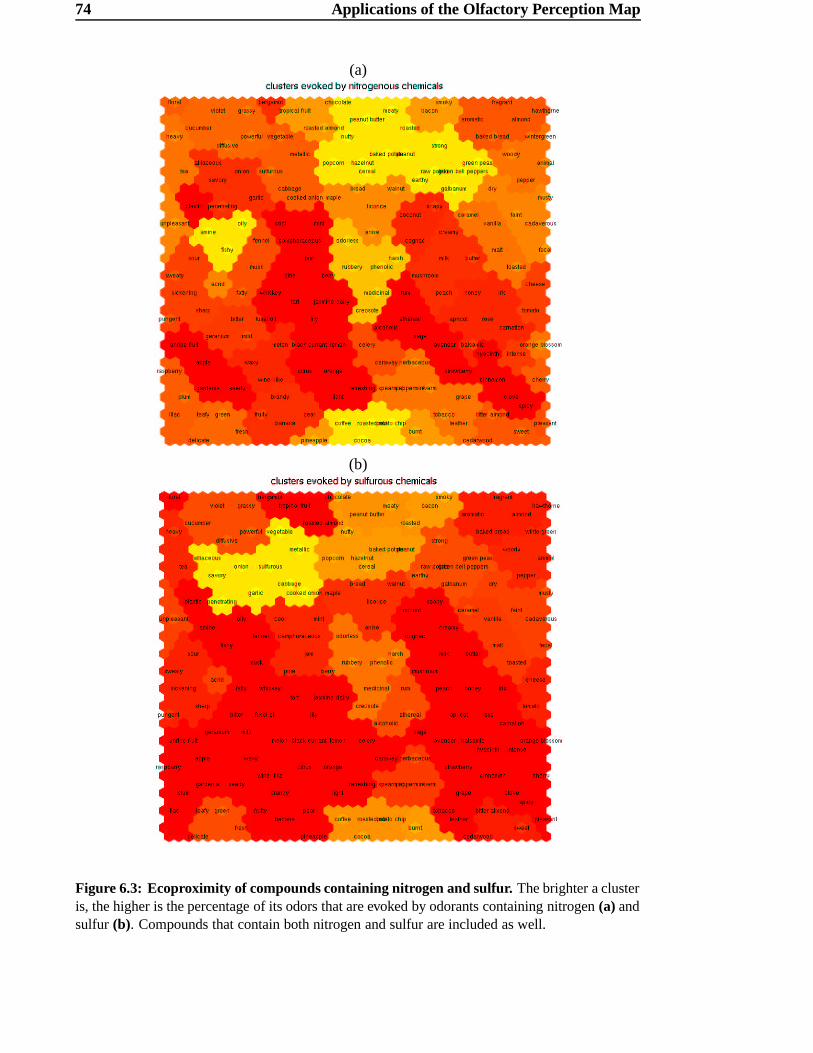
74 Applications of the Olfactory Perception Map
(a)
(b)
Figure 6.3: Ecoproximity of compounds containing nitrogen and sulfur. The brighter a clusteris, the higher is the percentage of its odors that are evoked by odorants containing nitrogen (a) andsulfur (b). Compounds that contain both nitrogen and sulfur are included as well.
6.3 Ecoproximity Hypothesis 75
using similar patterns, one would presume that this group of chemicals will only be able
to activate a related set of odors. In the following we will refer to this hypothesis as the
Ecoproximity Hypothesis.
Let us consider an intuitive test. We take the odor profiles of a group of compounds
and try to interpret the result in terms of a possible underlying order. If the odorants are
chosen using a characteristic that is relevant for their position in the odor space, we should
obtain a set of odors that more or less forms a group on the map. On the other hand, if
the odorants are chosen based on an irrelevant characteristic, the corresponding group of
odors will be spread all over the map.
We took all compounds that contain nitrogen and highlighted their odors on our map.
We did the same for compounds that contain sulfur. We obtained fascinating results.
In Figure 6.3.a, the result for compounds containing nitrogen can be seen. The shades
of the clusters represent the percentage of their odors that can be evoked by odorants con-
taining nitrogen. The brighter the cluster is, the higher the percentage of evoked odors.
Interestingly, these odors form very segregated groups. The structure seems to be
two-part and includes oily, nutty and earthy odors. In Figure 6.3.b, the same thing was
done for compounds containing sulfur. Accordingly, we obtain clearly segregated groups
containing smoky and garlic-like odors.
At first sight, one might be surprised that the two groups of nitrogen- and sulfur-
evoked odors are not totally disjoint. But we should not forget that there is an overlap
caused by chemicals that contain both nitrogen and sulfur. Other reasons that might lead
to an overlap are other common features that are not part of this small experiment. There
might be other characterizing elements, oxygen for example, that are contained in several
compounds, no matter whether they are nitrogen or sulfur compounds.
C H A P T E R 7
Conclusion and Future Work
7.1 Conclusion
It has been the main goal of this thesis to develop an infrastructure for generating a robust
and reliable map of the “olfactory perception space”. We used proven techniques to re-
duce highly complex psychophysical data systematically to a low-dimensional level that
may be much easier to explore for human scientists.
7.1.1 An infrastructure for quantifying Odor Space
In Chapter 2, the state of neuroscience research was outlined. Now we have got a feeling
for the problems that arise in understanding the sense of smell. In particular, it is still far
from clear what molecular characteristics lead to the corresponding odor perceptions.
Historical mapping attempts, like Henning’s “Odor Prism” [21], for example, try to
take the reasonable route of interpreting psychophysical observations to achieve a better
understanding of relationships between odors. A new and promising approach was pro-
posed by Chee-Ruiter [12]. She extracted information about odor similarities from large
existing databases and expressed them through a directed graph.
The idea was to project information about odor perceptions onto a map. This map
should function as an “odor wheel” similar in concept to a “color wheel”. Thus, this thesis
7.1 Conclusion 77
focused on the application and extension of this idea. We think that our mapping approach
will lead to new insights into the structure of the odor space, which, unfortunately, has so
far been just a continuum of unknown structure containing all odor perceptions.
Using a specially designed metric, multidimensional scaling and self-organizing maps,
an infrastructure has been proposed to visualize the odor space through a meaningful map.
The underlying techniques as well as related problems and restrictions were motivated and
discussed.
7.1.2 Quantifying odor quality data
As proposed by Chee-Ruiter [12], published databases of odorants (chemicals with a
smell) like the Aldrich Flavor and Fragrances Catalog [2] and Dravnieks Atlas of Odor
Character Profiles [17] were the source for odor information. According to Dravnieks
[16], a set of descriptors – like Aldrich’s – is a reliable and reproducible representation of
odor perception.
Chee-Ruiter used a data set based on the Aldrich Fragrances Catalog (including 851
chemicals using 278 odor descriptors) for a first mapping approach. We used the same
database for our new model of the odor space. We have shown that the subdimensional
distance KyÌ yields the intuitively most satisfying results for estimating dissimilarities be-
tween different odors. The measure KcÌ can be interpreted as a weighted version of Chee-
Ruiter’s Cross-Entropy Information I as proposed in Chapter 3.
7.1.3 Scaling of quantified data via MDS
Given a dissimilarity matrix, MDS projects these dissimilarities, which do not have to be
metric, into the nearest Euclidean space. MDS is a well-known method for dimension
reduction and graphical representation of multidimensional data.
The feature of non-metric scaling is essential for mapping the odor space because
78 Conclusion and Future Work
there is no indication that the odor space has a metric structure. In other words, we pro-
jected a space of unknown structure into an Euclidean space that best approximates this
structure.
MDS can also be used to estimate the dimensionality of a data set [32]. We found
evidence that the odor space seems to be approximately 32-dimensional. However, an
accurate answer to this question is by far not easy to give. This should thus be the topic
of further research.
7.1.4 Generating Kohonen Maps of scaled data
With the methods applied in Chapter 3 and 4 we obtained coordinates of odor descriptors
located in an Euclidean space that represents an approximation of “olfactory perception
space”. In Chapter 5, we used self-organizing maps to generate two-dimensional maps
from this high-dimensional Euclidean space.
The use of these maps is restricted by several criteria. Namely, there is the problem
of fragmented clusters that makes the definition of neighborhoods more complex. Some
clusters might be close to one another even if they are not neighbors on the Kohonen map.
We can solve this problem by consulting a second map that identifies the clusters using
numbers (see Figures 5.8 and 5.9). Furthermore, we have to be careful even if two clusters
are neighbors on the Kohonen map. It might be that they are not very close together in
terms of their high-dimensional representation. So we have to consult a third map to solve
this problem, the so-called U-matrix (see Figure 5.12).
7.1.5 Using the Olfactory Perception Map
The new approach of mapping the olfactory perception space enabled us to find several
interesting indications and ideas about odor perception. Beyond doubt, the most fasci-
nating new feature is the possibility to answer questions like: “How are apple, banana
and cherry ordered?” It is no longer true that such questions cannot be answered in odor
7.2 Future Work 79
perception.
Furthermore, we showed that the directed graph approach by Chee-Ruiter had al-
ready led to reasonable hypotheses, for which we could now formulate much stronger
arguments. In particular, we were able to show strong evidence for the ecoproximity hy-
pothesis.
In other words, we have found evidence that the olfactory system processes metaboli-
cally similar odorants using similar neural activation patterns. We were able to show that
similar odorants evoke only related sets of odors. Thus, it seems as if these groups of
chemicals are processed using similar neural activation patterns.
7.2 Future Work
Even though the description “a color wheel for odors” is very evocative, we are not trying
to find a continuum of odors. The question is whether we are able to create a meaningful
map that expresses all the information we can obtain from experiments. On this map, we
will then be able to test ideas and models that might represent the “truth” about odor space.
One of the striking problems in evaluating such a model is that we do not even have
an idea of what the reality looks like. We simply do not know how the “olfactory percep-
tion space” is structured. So it is very difficult to say something about potential errors in
estimating similarities between odors.
However, this is the goal of modeling the odor space. The model should incorporate
as much information as possible and tries to model real olfactory perception as well as
possible.
What does the “olfactory perception map” represent? Maybe we can already see a
map of the pyriform cortex. Can we find some similarities between our psychophysical
80 Conclusion and Future Work
model and the odor space hypotheses by Hopfield [23]? Or the map will just turn out to
be an example of how insufficiently olfactory perception is categorized by odor profiles.
In any case, it is essential to search for evidence about the correctness or falseness of
the model when compared with the real world. Otherwise the work presented here will
become worthless.
7.2.1 Odor Perception vs. Face Recognition
There is a striking analogy between odor and face perception. People often have problems
describing faces, but they are very adept at discriminating faces. This is why the police
works with photofit techniques. It is much more fruitful to ask persons if they know a
face than to ask them for a detailed description.
With odorants, the case is similar. Asking people for their description of an odorant
often leads to a typical answer like “I know this odorant.” followed by a more or less
inadequate description. So when people have to characterize odorants, they are given a
characterization form — just as for photofit techniques — and only have to judge whether
or not a certain smell fits to certain odor descriptors.
We could probably learn from results in face perception, since we know more about
face perception than about odor perception. For faces, there are already sophisticated
models that express a multi-dimensional face space [24]. Of course there is a physical
continuum in face perception. We can physically measure similarities, e.g. eye distance
and hair color. In odor perception, we do not know if this is possible. Therefore, in face
perception, we can easily distinguish between different features and different values of
the same feature.
Let us assume we apply the presented infrastructure to a psychophysical face database.
The resulting map might look like the one in Figure 7.1. big eyes and round face would
probably be quite close to cute, while bushy eyebrows would be close to brown eyes, be-
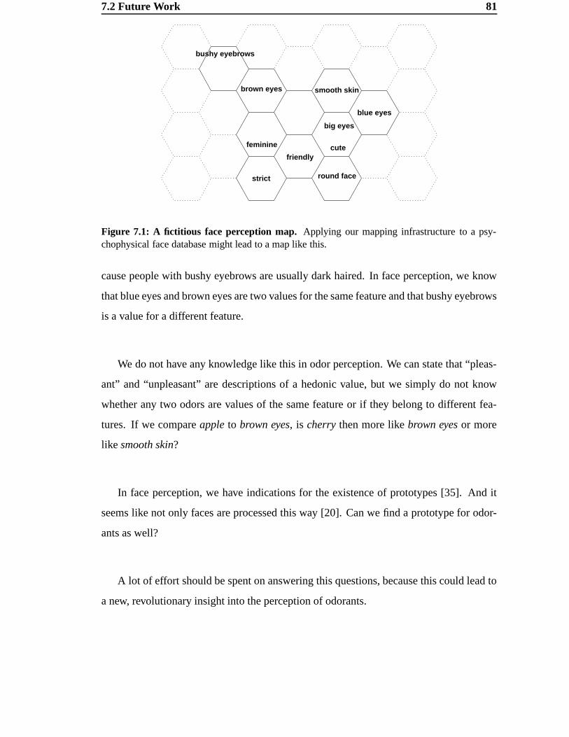
7.2 Future Work 81
round face
bushy eyebrows
cute
big eyes
brown eyes
feminine
friendly
smooth skin
blue eyes
strict
Figure 7.1: A fictitious face perception map. Applying our mapping infrastructure to a psy-chophysical face database might lead to a map like this.
cause people with bushy eyebrows are usually dark haired. In face perception, we know
that blue eyes and brown eyes are two values for the same feature and that bushy eyebrows
is a value for a different feature.
We do not have any knowledge like this in odor perception. We can state that “pleas-
ant” and “unpleasant” are descriptions of a hedonic value, but we simply do not know
whether any two odors are values of the same feature or if they belong to different fea-
tures. If we compare apple to brown eyes, is cherry then more like brown eyes or more
like smooth skin?
In face perception, we have indications for the existence of prototypes [35]. And it
seems like not only faces are processed this way [20]. Can we find a prototype for odor-
ants as well?
A lot of effort should be spent on answering this questions, because this could lead to
a new, revolutionary insight into the perception of odorants.
82 Conclusion and Future Work
7.2.2 Dimensionality of Odor Space
Future work should definitively also address the problem of dimensionality. On one hand,
this problem corresponds strongly with the feature extraction problem we just discussed,
because the number of features equals the dimension of the odor space. On the other
hand, we will learn a lot about the complexity of the olfactory cortex and especially the
structures between the bulb and the cortex.
For our model and the underlying data, a space with a dimensionality of approxi-
mately 32 dimensions seemed to be sufficient. But we should not forget that this estimate
is only a rough guess resulting from the scatter diagrams. It should be possible to increase
the precision of such an estimate significantly.
Especially the extraction of independent subsets of odors might lead to new revela-
tions about the general organization of odor perception space.
We used a standard MDS method. There are different possibilities to scale multi-
dimensional data. Most of them, Sammon mapping [44], for example, have the same
mathematical background and therefore differ only in some degree of relaxation. But
there are some new approaches using linear embedding [43] and geometric frameworks
[49] that might be able to estimate the intrinsic dimensionality of odor space better than
MDS.
7.2.3 Psychophysical Experiments
Last but not least, a small experiment should be mentioned here. Although the number
of subjects as well as the number of trials was not sufficient by far to obtain significant
results, it was a very interesting experience — especially for the author — to get an in-
sight into planning and performing a psychophysical experiment. Besides, the results
emphasized the necessity of psychophysical experiments as a practical contribution to the
mapping of odor space.
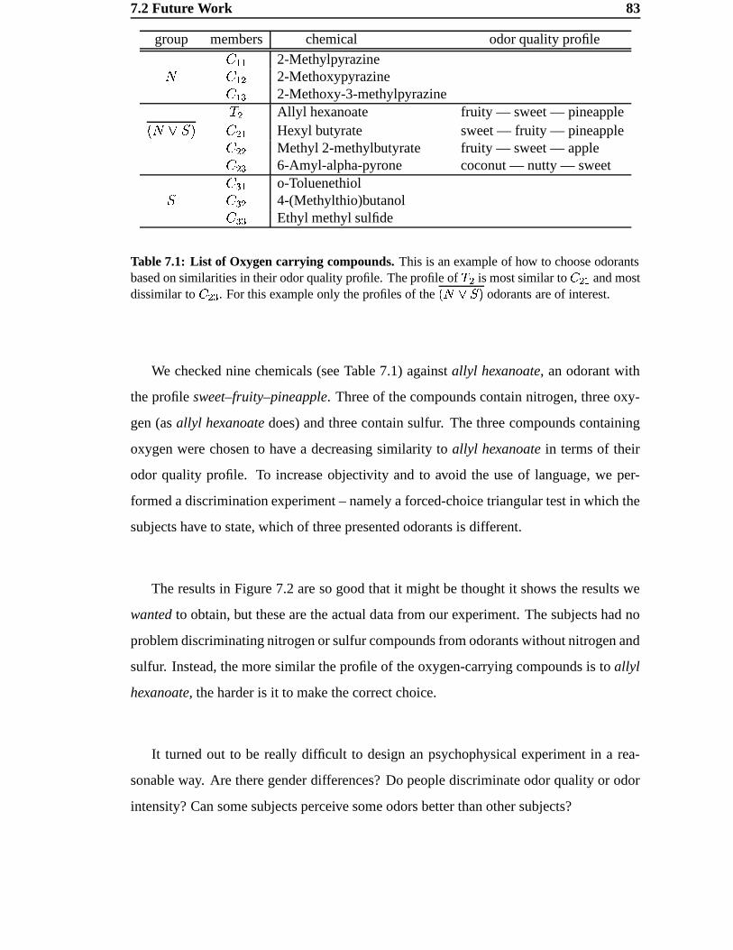
7.2 Future Work 83
group members chemical odor quality profile� BJB 2-Methylpyrazine] � B � 2-Methoxypyrazine� B � 2-Methoxy-3-methylpyrazine^ � Allyl hexanoate fruity — sweet — pineapple� ]`_ba � � � B Hexyl butyrate sweet — fruity — pineapple� �J� Methyl 2-methylbutyrate fruity — sweet — apple� � � 6-Amyl-alpha-pyrone coconut — nutty — sweet�P� B o-Toluenethiola �P� � 4-(Methylthio)butanol�P�J� Ethyl methyl sulfide
Table 7.1: List of Oxygen carrying compounds. This is an example of how to choose odorantsbased on similarities in their odor quality profile. The profile of c � is most similar to d � B and mostdissimilar to d � � . For this example only the profiles of the fehg6ij� odorants are of interest.
We checked nine chemicals (see Table 7.1) against allyl hexanoate, an odorant with
the profile sweet–fruity–pineapple. Three of the compounds contain nitrogen, three oxy-
gen (as allyl hexanoate does) and three contain sulfur. The three compounds containing
oxygen were chosen to have a decreasing similarity to allyl hexanoate in terms of their
odor quality profile. To increase objectivity and to avoid the use of language, we per-
formed a discrimination experiment – namely a forced-choice triangular test in which the
subjects have to state, which of three presented odorants is different.
The results in Figure 7.2 are so good that it might be thought it shows the results we
wanted to obtain, but these are the actual data from our experiment. The subjects had no
problem discriminating nitrogen or sulfur compounds from odorants without nitrogen and
sulfur. Instead, the more similar the profile of the oxygen-carrying compounds is to allyl
hexanoate, the harder is it to make the correct choice.
It turned out to be really difficult to design an psychophysical experiment in a rea-
sonable way. Are there gender differences? Do people discriminate odor quality or odor
intensity? Can some subjects perceive some odors better than other subjects?
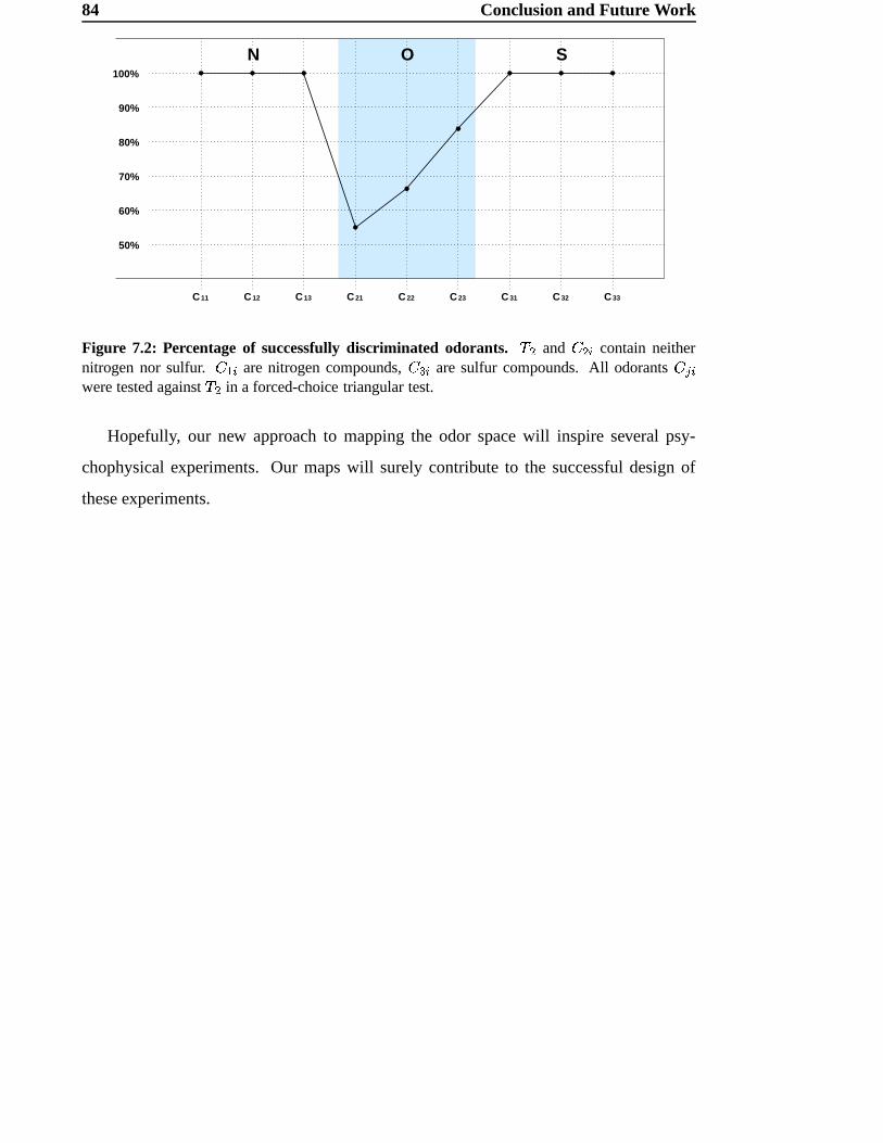
84 Conclusion and Future Work
100%
50%
60%
70%
80%
90%
C 11 C 13 C 21 C 22 C 23 C 31 C 32 C 33C 12
ON S
Figure 7.2: Percentage of successfully discriminated odorants. c � and d � l contain neithernitrogen nor sulfur. d B l are nitrogen compounds, d � l are sulfur compounds. All odorants d © lwere tested against c � in a forced-choice triangular test.
Hopefully, our new approach to mapping the odor space will inspire several psy-
chophysical experiments. Our maps will surely contribute to the successful design of
these experiments.
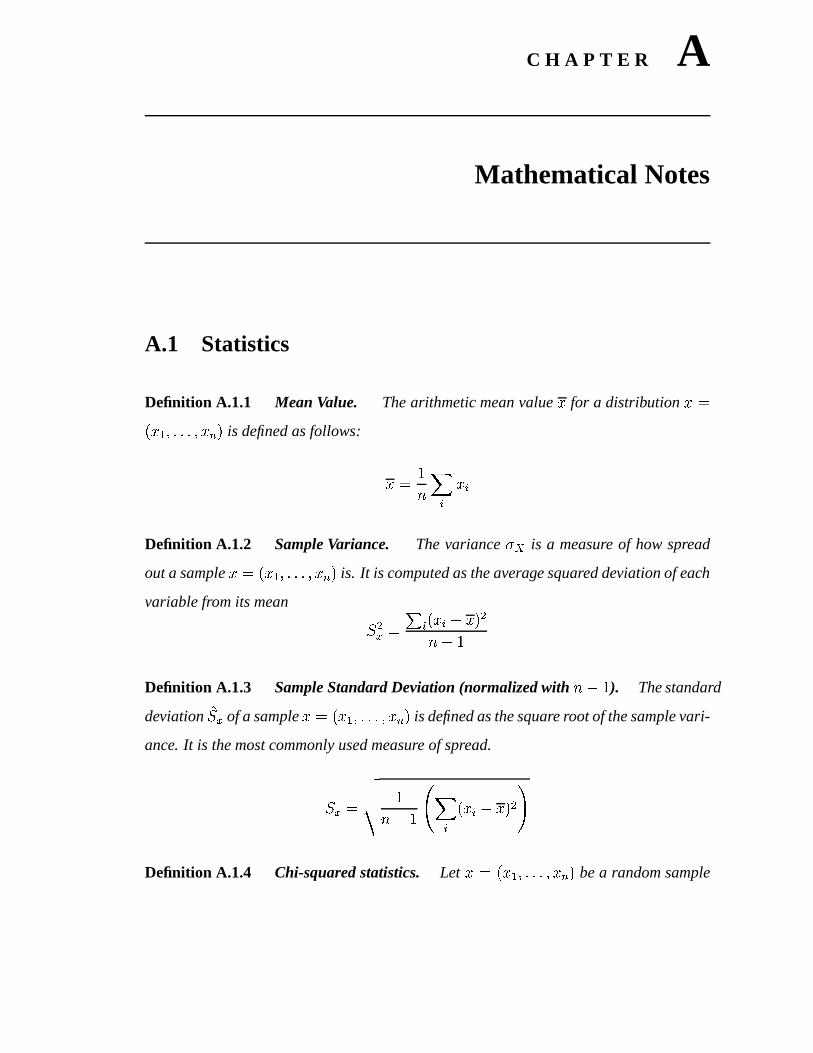
C H A P T E R A
Mathematical Notes
A.1 Statistics
Definition A.1.1 Mean Value. The arithmetic mean value * for a distribution * .�Í* B "#�#�H�H"¼* D � is defined as follows: * . �� j,l * lDefinition A.1.2 Sample Variance. The variance P\k is a measure of how spread
out a sample * . �Í* B "H�#�#�H"`* D � is. It is computed as the average squared deviation of each
variable from its mean a �> . � l �Í* l � *,�ü�� � �Definition A.1.3 Sample Standard Deviation (normalized with �:� � ). The standard
deviation la > of a sample * . � * B "#�H�#�H"¼* D � is defined as the square root of the sample vari-
ance. It is the most commonly used measure of spread.
a > . ���� �� �û� n jLl �Í* l � *,� � qDefinition A.1.4 Chi-squared statistics. Let * . �Í* B "#�#�H��"¼* D � be a random sample
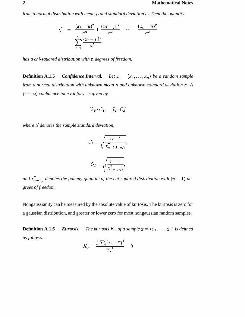
2 Mathematical Notes
from a normal distribution with mean @ and standard deviation P . Then the quantity
m � . �Í* B �K@8���P � \ � * � �K@����P � \Å7%7%7#\ �Í* D �=@8���P �. Dj l(¹ B � * l �n@8���P �has a chi-squared distribution with � degrees of freedom.
Definition A.1.5 Confidence Interval. Let * . �Í* B "H�#�#�z"¼* D � be a random sample
from a normal distribution with unknown mean @ and unknown standard deviation P . A���ª��� � confidence interval for P is given by� a >�7$� B " a >õ7$� � �where
adenotes the sample standard deviation,� B . �:� �m �D ñ B � B ñpo r � "� � . �:� �m �D ñ B � o r � "
and m �D ñ Brq s denotes the gammy-quantile of the chi-squared distribution with ���v�0�$� de-
grees of freedom.
Nongaussianity can be measured by the absolute value of kurtosis. The kurtosis is zero for
a gaussian distribution, and greater or lower zero for most nongaussian random samples.
Definition A.1.6 Kurtosis. The kurtosis te> of a sample * . �Í* B "#�#�#��"¼* D � is defined
as follows: t > . BD � l �Í* l � *é� a > ��¶
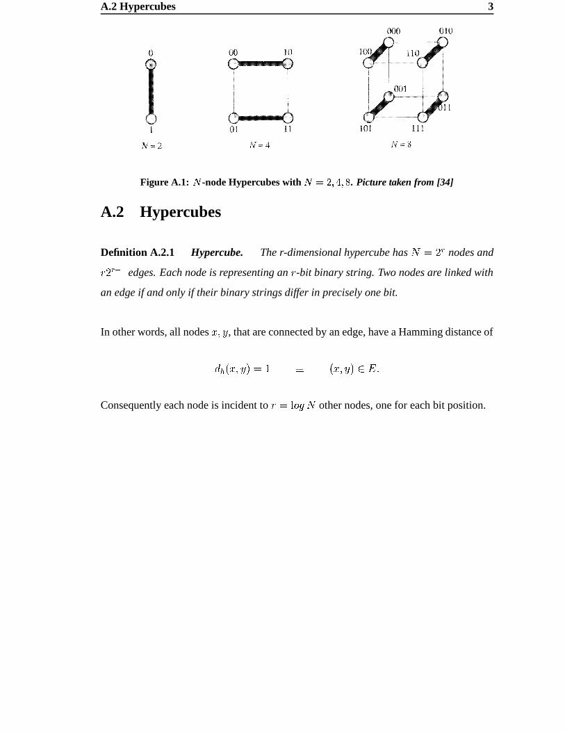
A.2 Hypercubes 3
Figure A.1: e -node Hypercubes with eu�þG�r�v�w� . Picture taken from [34]
A.2 Hypercubes
Definition A.2.1 Hypercube. The r-dimensional hypercube has] . �vx nodes and{��yx ñ B edges. Each node is representing an { -bit binary string. Two nodes are linked with
an edge if and only if their binary strings differ in precisely one bit.
In other words, all nodes *8" V , that are connected by an edge, have a Hamming distance ofK ' �Í*8" V � . � z � *8" V �[ub{e�Consequently each node is incident to { . å ;�| ] other nodes, one for each bit position.
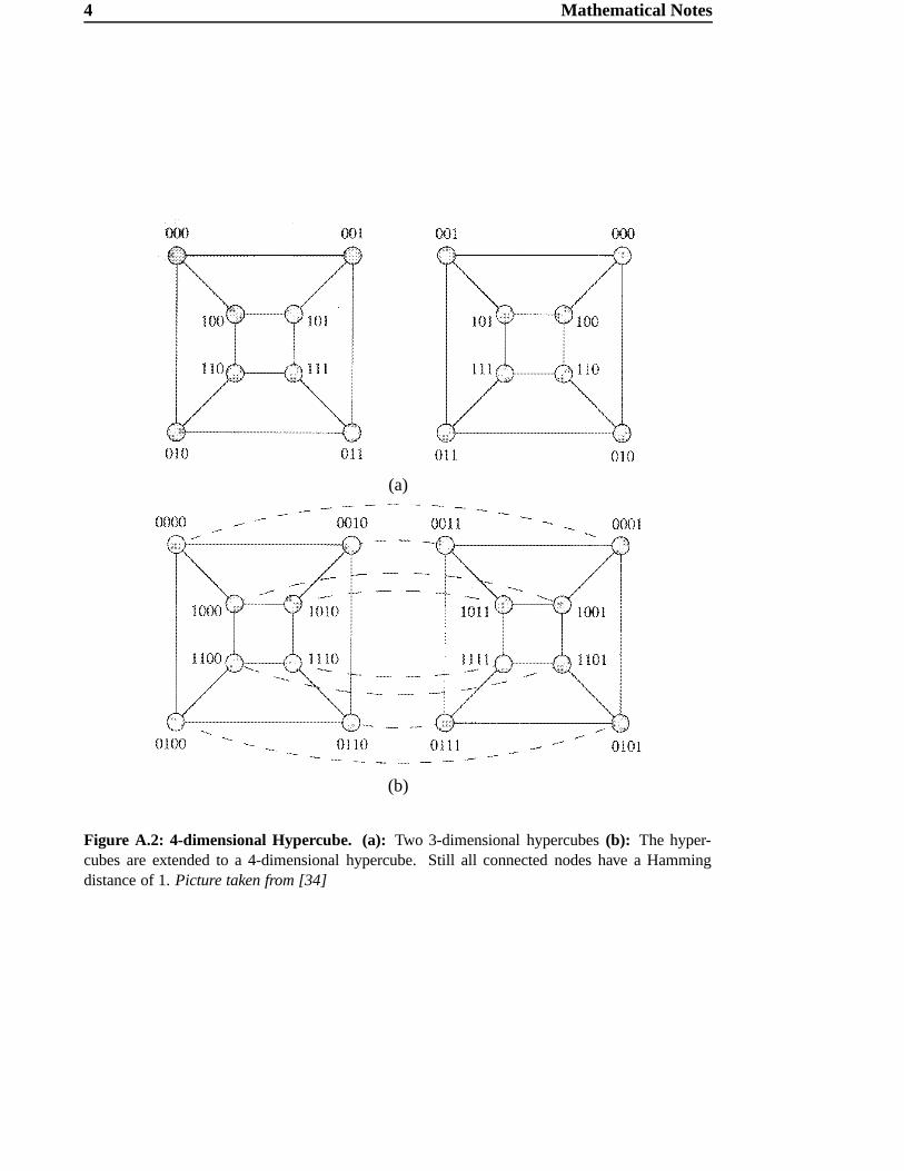
4 Mathematical Notes
(a)
(b)
Figure A.2: 4-dimensional Hypercube. (a): Two 3-dimensional hypercubes (b): The hyper-cubes are extended to a 4-dimensional hypercube. Still all connected nodes have a Hammingdistance of 1. Picture taken from [34]

C H A P T E R B
Labels and Maps
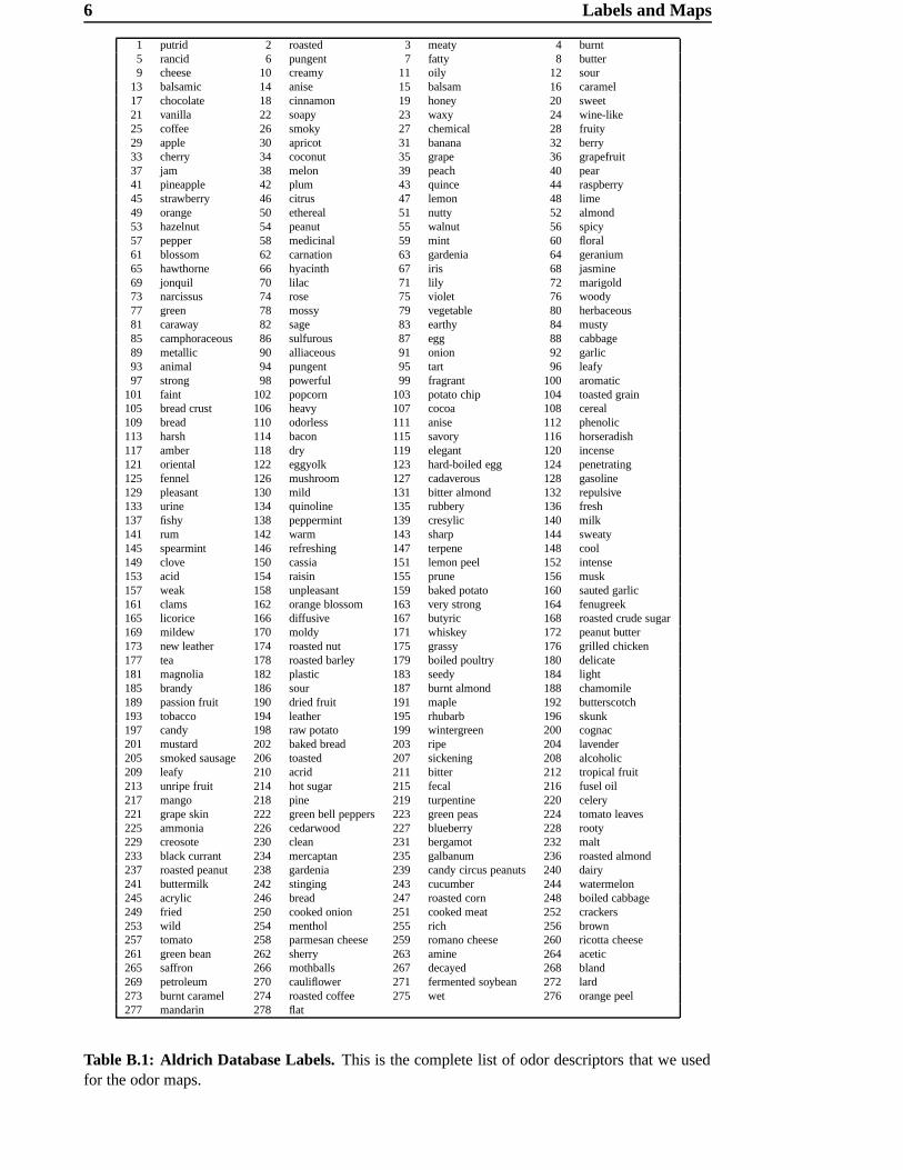
6 Labels and Maps
1 putrid 2 roasted 3 meaty 4 burnt5 rancid 6 pungent 7 fatty 8 butter9 cheese 10 creamy 11 oily 12 sour
13 balsamic 14 anise 15 balsam 16 caramel17 chocolate 18 cinnamon 19 honey 20 sweet21 vanilla 22 soapy 23 waxy 24 wine-like25 coffee 26 smoky 27 chemical 28 fruity29 apple 30 apricot 31 banana 32 berry33 cherry 34 coconut 35 grape 36 grapefruit37 jam 38 melon 39 peach 40 pear41 pineapple 42 plum 43 quince 44 raspberry45 strawberry 46 citrus 47 lemon 48 lime49 orange 50 ethereal 51 nutty 52 almond53 hazelnut 54 peanut 55 walnut 56 spicy57 pepper 58 medicinal 59 mint 60 floral61 blossom 62 carnation 63 gardenia 64 geranium65 hawthorne 66 hyacinth 67 iris 68 jasmine69 jonquil 70 lilac 71 lily 72 marigold73 narcissus 74 rose 75 violet 76 woody77 green 78 mossy 79 vegetable 80 herbaceous81 caraway 82 sage 83 earthy 84 musty85 camphoraceous 86 sulfurous 87 egg 88 cabbage89 metallic 90 alliaceous 91 onion 92 garlic93 animal 94 pungent 95 tart 96 leafy97 strong 98 powerful 99 fragrant 100 aromatic
101 faint 102 popcorn 103 potato chip 104 toasted grain105 bread crust 106 heavy 107 cocoa 108 cereal109 bread 110 odorless 111 anise 112 phenolic113 harsh 114 bacon 115 savory 116 horseradish117 amber 118 dry 119 elegant 120 incense121 oriental 122 eggyolk 123 hard-boiled egg 124 penetrating125 fennel 126 mushroom 127 cadaverous 128 gasoline129 pleasant 130 mild 131 bitter almond 132 repulsive133 urine 134 quinoline 135 rubbery 136 fresh137 fishy 138 peppermint 139 cresylic 140 milk141 rum 142 warm 143 sharp 144 sweaty145 spearmint 146 refreshing 147 terpene 148 cool149 clove 150 cassia 151 lemon peel 152 intense153 acid 154 raisin 155 prune 156 musk157 weak 158 unpleasant 159 baked potato 160 sauted garlic161 clams 162 orange blossom 163 very strong 164 fenugreek165 licorice 166 diffusive 167 butyric 168 roasted crude sugar169 mildew 170 moldy 171 whiskey 172 peanut butter173 new leather 174 roasted nut 175 grassy 176 grilled chicken177 tea 178 roasted barley 179 boiled poultry 180 delicate181 magnolia 182 plastic 183 seedy 184 light185 brandy 186 sour 187 burnt almond 188 chamomile189 passion fruit 190 dried fruit 191 maple 192 butterscotch193 tobacco 194 leather 195 rhubarb 196 skunk197 candy 198 raw potato 199 wintergreen 200 cognac201 mustard 202 baked bread 203 ripe 204 lavender205 smoked sausage 206 toasted 207 sickening 208 alcoholic209 leafy 210 acrid 211 bitter 212 tropical fruit213 unripe fruit 214 hot sugar 215 fecal 216 fusel oil217 mango 218 pine 219 turpentine 220 celery221 grape skin 222 green bell peppers 223 green peas 224 tomato leaves225 ammonia 226 cedarwood 227 blueberry 228 rooty229 creosote 230 clean 231 bergamot 232 malt233 black currant 234 mercaptan 235 galbanum 236 roasted almond237 roasted peanut 238 gardenia 239 candy circus peanuts 240 dairy241 buttermilk 242 stinging 243 cucumber 244 watermelon245 acrylic 246 bread 247 roasted corn 248 boiled cabbage249 fried 250 cooked onion 251 cooked meat 252 crackers253 wild 254 menthol 255 rich 256 brown257 tomato 258 parmesan cheese 259 romano cheese 260 ricotta cheese261 green bean 262 sherry 263 amine 264 acetic265 saffron 266 mothballs 267 decayed 268 bland269 petroleum 270 cauliflower 271 fermented soybean 272 lard273 burnt caramel 274 roasted coffee 275 wet 276 orange peel277 mandarin 278 flat
Table B.1: Aldrich Database Labels. This is the complete list of odor descriptors that we usedfor the odor maps.
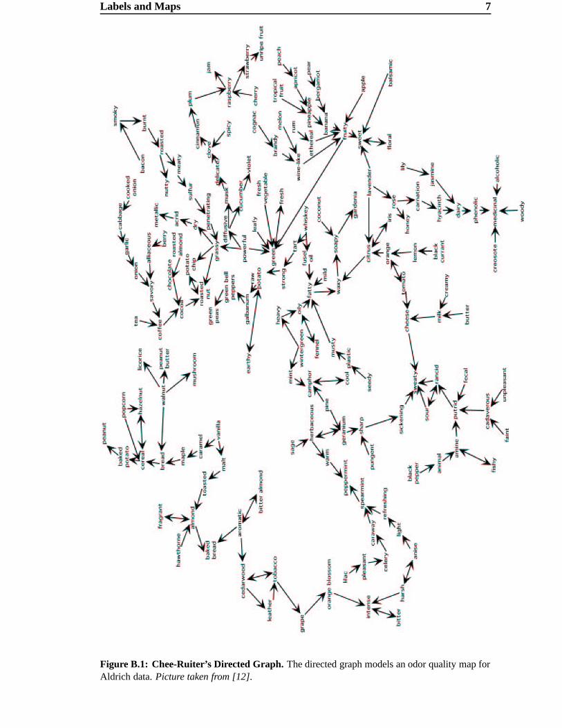
Labels and Maps 7
Figure B.1: Chee-Ruiter’s Directed Graph. The directed graph models an odor quality map forAldrich data. Picture taken from [12].
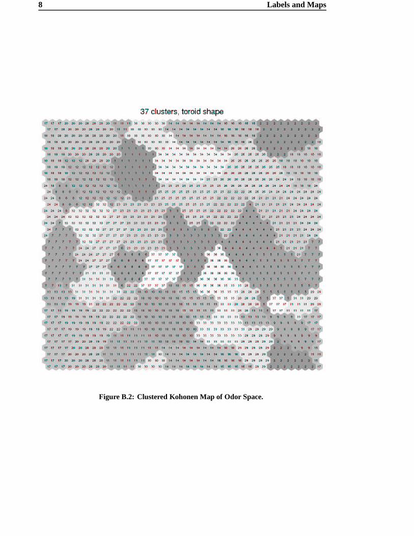
8 Labels and Maps
Figure B.2: Clustered Kohonen Map of Odor Space.
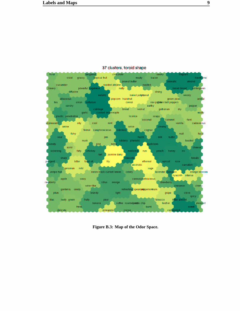
Labels and Maps 9
Figure B.3: Map of the Odor Space.
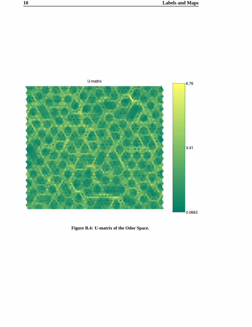
10 Labels and Maps
Figure B.4: U-matrix of the Odor Space.
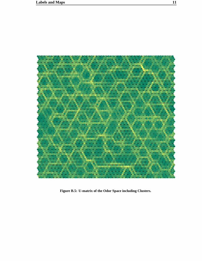
Labels and Maps 11
Figure B.5: U-matrix of the Odor Space including Clusters.
List of Figures
1.1 Data flow through the mapping infrastructure . . . . . . . . . . . . . . 6
2.1 Schematic view of the human nose . . . . . . . . . . . . . . . . . . . . 9
2.2 Olfactory Receptor Neuron. . . . . . . . . . . . . . . . . . . . . . . . . 10
2.3 Olfactory Epithelium. . . . . . . . . . . . . . . . . . . . . . . . . . . . 11
2.4 Olfactory Bulb . . . . . . . . . . . . . . . . . . . . . . . . . . . . . . 12
2.5 Henning’s odor prism . . . . . . . . . . . . . . . . . . . . . . . . . . . 14
2.6 Part of Chee-Ruiter’s odor graph . . . . . . . . . . . . . . . . . . . . . 16
3.1 Stuffing of the observation vectors . . . . . . . . . . . . . . . . . . . . 28
3.2 SD matrix for aldrich database . . . . . . . . . . . . . . . . . . . . . . 34
4.1 Reconstructing points from a distance matrix . . . . . . . . . . . . . . 37
4.2 Sketch of some points . . . . . . . . . . . . . . . . . . . . . . . . . . . 40
4.3 Sample Run of MDS . . . . . . . . . . . . . . . . . . . . . . . . . . . 42
4.4 Scatter Plot of 2D-MDS on Aldrich database . . . . . . . . . . . . . . . 44
4.5 Map resulting from 2D MDS based on Aldrich database . . . . . . . . . 45
4.6 Scatter Plots of 8D- and 16D-MDS on Aldrich database . . . . . . . . . 48
4.7 Scatter Plot of 32D- and 64D-MDS on Aldrich database . . . . . . . . . 49
4.8 Stress values for different Dimensions . . . . . . . . . . . . . . . . . . 50
LIST OF FIGURES 13
4.9 Comparison of 16D, 32D and 42D MDS results . . . . . . . . . . . . . 53
5.1 Abstract Kohonen model . . . . . . . . . . . . . . . . . . . . . . . . . 56
5.2 Flat torus vs. doughnut surface . . . . . . . . . . . . . . . . . . . . . . 57
5.3 Competitive Learning of SOM . . . . . . . . . . . . . . . . . . . . . . 59
5.4 2D example: training set for SOM . . . . . . . . . . . . . . . . . . . . 61
5.5 2D example: SOM initialization . . . . . . . . . . . . . . . . . . . . . 61
5.6 2D example: SOM after training . . . . . . . . . . . . . . . . . . . . . 62
5.7 Unified distance matrix. . . . . . . . . . . . . . . . . . . . . . . . . . . 63
5.8 Clustered Kohonen Map of Odor Space . . . . . . . . . . . . . . . . . 64
5.9 Fragmented Clusters on the Kohonen Map of Odor Space . . . . . . . . 65
5.10 Surface of Odor Space . . . . . . . . . . . . . . . . . . . . . . . . . . 66
5.11 Map of the Odor Space . . . . . . . . . . . . . . . . . . . . . . . . . . 67
5.12 U-matrix of the Odor Space . . . . . . . . . . . . . . . . . . . . . . . . 68
6.1 A group of herbaceous odors . . . . . . . . . . . . . . . . . . . . . . . 71
6.2 Groups of unpleasant and nutty odors . . . . . . . . . . . . . . . . . . 73
6.3 Ecoproximity of compounds containing N and S . . . . . . . . . . . . . 74
7.1 A fictitious face perception map . . . . . . . . . . . . . . . . . . . . . 81
7.2 Percentage of successfully discriminated odorants . . . . . . . . . . . . 84
A.1]
-node Hypercubes with] . �c"¼ÃÇ"C . . . . . . . . . . . . . . . . . . 3
A.2 4-dimensional Hypercube . . . . . . . . . . . . . . . . . . . . . . . . . 4
B.1 Chee-Ruiter’s Directed Graph . . . . . . . . . . . . . . . . . . . . . . 7
B.2 Clustered Kohonen Map of Odor Space . . . . . . . . . . . . . . . . . 8

14 LIST OF FIGURES
B.3 Map of the Odor Space . . . . . . . . . . . . . . . . . . . . . . . . . . 9
B.4 U-matrix of the Odor Space . . . . . . . . . . . . . . . . . . . . . . . . 10
B.5 U-matrix of the Odor Space including Clusters . . . . . . . . . . . . . 11
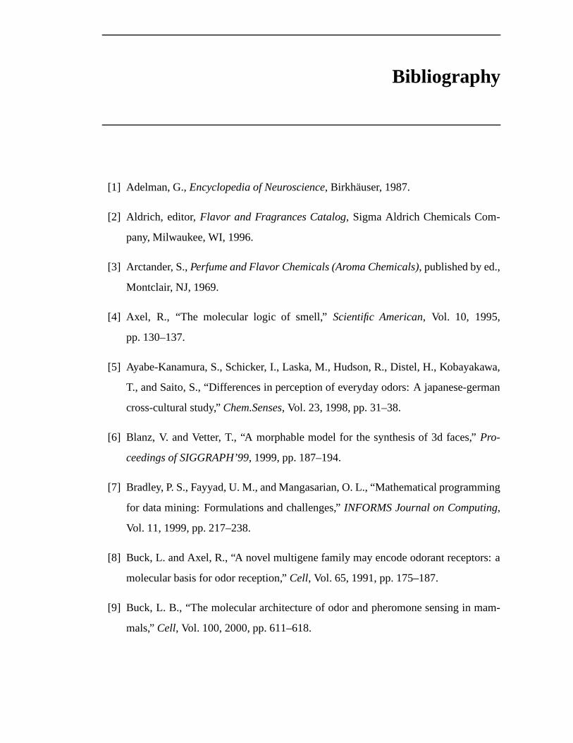
Bibliography
[1] Adelman, G., Encyclopedia of Neuroscience, Birkhauser, 1987.
[2] Aldrich, editor, Flavor and Fragrances Catalog, Sigma Aldrich Chemicals Com-
pany, Milwaukee, WI, 1996.
[3] Arctander, S., Perfume and Flavor Chemicals (Aroma Chemicals), published by ed.,
Montclair, NJ, 1969.
[4] Axel, R., “The molecular logic of smell,” Scientific American, Vol. 10, 1995,
pp. 130–137.
[5] Ayabe-Kanamura, S., Schicker, I., Laska, M., Hudson, R., Distel, H., Kobayakawa,
T., and Saito, S., “Differences in perception of everyday odors: A japanese-german
cross-cultural study,” Chem.Senses, Vol. 23, 1998, pp. 31–38.
[6] Blanz, V. and Vetter, T., “A morphable model for the synthesis of 3d faces,” Pro-
ceedings of SIGGRAPH’99, 1999, pp. 187–194.
[7] Bradley, P. S., Fayyad, U. M., and Mangasarian, O. L., “Mathematical programming
for data mining: Formulations and challenges,” INFORMS Journal on Computing,
Vol. 11, 1999, pp. 217–238.
[8] Buck, L. and Axel, R., “A novel multigene family may encode odorant receptors: a
molecular basis for odor reception,” Cell, Vol. 65, 1991, pp. 175–187.
[9] Buck, L. B., “The molecular architecture of odor and pheromone sensing in mam-
mals,” Cell, Vol. 100, 2000, pp. 611–618.
16 Bibliography
[10] Cain, W. S., “History of research on smell,” E. C. Carterette and M. P. Friedmann
(Eds.), Handbook of Perception, Vol. VIA: Tasting and Smelling, 1978, pp. 197–
243.
[11] Cain, W. S., de Wijk, R., Lulejian, C., Schiet, F., and See, L., “Odor identification:
Perceptual and semantic dimensions,” Chem.Senses, Vol. 23, 1998, pp. 309–326.
[12] Chee-Ruiter, C. W. J., The Biological Sense of Smell: Olfactory Search Behavior
and a Metabolic View for Olfactory Perception, Ph.D. thesis, California Institute of
Technology, Pasadena, CA, 2000.
[13] Copson, E. T., Metric Spaces, Cambridge University Press, Cambridge, 1968.
[14] Darnell, J., Molecular Cell Biology, Scientific American Books, 1995.
[15] Daum, R. F., Sekinger, B., Kobal, G., and Lang, C. J. G., “Riechprufung mit sniffin’
sticks zur klinischen diagnostik des morbus parkinson,” Nervenarzt, Vol. 71, 2000,
pp. 643–650.
[16] Dravnieks, A., “Odor quality: Semantically generated multidimensional profiles are
stable,” Science, Vol. 218, 1982, pp. 799–801.
[17] Dravnieks, A., Atlas of Odor Character Profiles, Data Series DS 61, ASTM,
Philadelphia, PA, 1985.
[18] Faloutsos, C. and Lin, K., “Fastmap: A fast algorithm for indexing, data-mining and
visualization of tradditional and multimedia datasets,” Proceedings of 1995 ACM
SIGMOD, Vol. 24, 1995, pp. 163–174.
[19] Furia, T. and Bellanca, N., Fenaroli’s Handbook of Flavor Ingredients, CRC Press,
Boca Raton, FL, 1994.
[20] Gauthier, I., Skudlarski, P., Gore, J. C., and Anderson, A. W., “Expertise for cars
and birds recruits brain areas involved in face recognition,” Nature Neuroscience,
Vol. 3, 2000, pp. 191–197.
[21] Henning, H., Der Geruch, Barth, Leipzig, 1916.
Bibliography 17
[22] Henrysson, S., Applicability of factor analysis in the behavioral sciences, Almquist
& Wiksell, Stockholm, 1957.
[23] Hopfield, J. J., “Odor space and olfactory processing: Collective algorithms and
neural implementation,” PNAS, Vol. 96, October 1999, pp. 12506–12511.
[24] Hurlbert, A., “Trading faces,” Nature Neuroscience, Vol. 4, 2001, pp. 3–5.
[25] Jain, A. K. and Dubes, R. C., Algorithms for clustering data, Prentice Hall Advanced
Reference Series: Computer Science, New Jersey, 1988.
[26] Jolliffe, I. T., Principal Component Analysis, Springer-Verlag, New York, 1986.
[27] Kanwisher, N., “Domain specifity in face perception,” Nature Neuroscience, Vol. 3,
2000, pp. 759–763.
[28] Kaski, S., Data Exploration using Self-Organizing Maps, D.sc. (tech), Helsinki
University of Technology, Finland, March 1997, Acta Polytechnica Scandinavica,
Mathematics, Computing and Management in Engineering Series No. 82.
[29] Kohonen, T., Self-Organizing Maps, Springer-Verlag, Berlin, Heidelberg, 1995.
[30] Kruskal, J. B., “Multidimensional scaling by optimizing goodness-of-fit to a non-
metric hypothesis,” Psychometrika, Vol. 29, 1964, pp. 1–29.
[31] Kruskal, J. B., “Non-metric multidimensional scaling: A numerical method,” Psy-
chometrika, Vol. 29, 1964, pp. 115–129.
[32] Kruskal, J. B. and Wish, M., Multidimensional Scaling, Sage Publications, Beverly
Hills, CA, 1978.
[33] Laska, M., Ayabe-Kanamura, S., Hubener, F., and Saito, S., “Olfactory discrimi-
nation ability for aliphatic odorants as a function of oxygen moiety,” Chem.Senses,
Vol. 25, 2000, pp. 189–197.
[34] Leighton, F. T., Introduction to parallel algorithms and achitectures: arrays, trees,
hypercubes, Morgan Kaufmann Publishers, Inc., San Mateo, CA, 1992.
18 Bibliography
[35] Leopold, D. A., O’Toole, A. J., Vetter, T., and Blanz, V., “Prototype-referenced
shape encoding revealed by high-level aftereffects,” Nature Neuroscience, Vol. 4,
2001, pp. 89–94.
[36] Levine, M. W., Fundamentals of Sensation and Perception, Oxford University Press,
New York, 3rd ed., 2001.
[37] Malnic, B., Hirono, J., Sato, T., and Buck, L. B., “Combinatorical receptor codes for
odors,” Cell, Vol. 96, 1999, pp. 713–723.
[38] Miclet, L., Structural Methods in Pattern Recognition, Springer-Verlag, New York,
1986.
[39] Mumford, D., “Mathematical theories of shape: Do they model perception?” SPIE
Geometric Methods in Computer Vision, Vol. 1570, 1991, pp. 2–10.
[40] Ohloff, G., Scent and Fragrances, Springer Verlag, 1993.
[41] Olsson, M. J. and Cain, W. S., “Psychometrics of odor quality discrimination:
Method for threshold determination,” Chem.Senses, Vol. 25, 2000, pp. 493–499.
[42] Romney, A. K., Shepard, R. N., and Nerlove, S. B., Multidimensional Scaling: The-
ory and Applications in the Behavioural Sciences, Volume II – Applications, Seminar
Press, New York, 1972.
[43] Roweis, S. T. and Saul, L. K., “Nonlinear dimensionality reduction by locally linear
embedding,” Science, Vol. 290, December 2000, pp. 2323–2326.
[44] Sammon Jr., J. W., “A nonlinear mapping for data structure analysis,” IEEE Trans-
actions on Computers, Vol. C-18, 1969, pp. 401–409.
[45] Schiffman, H. R., Sensation and Perception - An Integrated Approach, John Wiley
& Sons, Inc., New York, 4th ed., 1996.
[46] Schiffman, S. S., “Contributions to the physicochemical dimensions of odor: a psy-
chophysical approach,” Ann N Y Acad Sci., Vol. 237, September 1974, pp. 164–183.
[47] Schiffman, S. S., Reynolds, M. L., and Young, F. W., Introduction to Multidimen-
sional Scaling, Academic Press, 1981.
Bibliography 19
[48] Shepard, R. N., Romney, A. K., and Nerlove, S. B., Multidimensional Scaling: The-
ory and Applications in the Behavioural Sciences, Volume I – Theory, Seminar Press,
New York, 1972.
[49] Tenenbaum, J. B., de Silva, V., and Langford, J. C., “A global geometric framework
for nonlinear dimensionality reduction,” Science, Vol. 290, 2000, pp. 2319–2323.
[50] Vesanto, J., Himberg, J., Alhoniemi, E., and Parhankangas, J., “Self-organizing map
in matlab: the som toolbox,” Proceedings of the Matlab DSP Conference 1999,
November 1999, pp. 35–40.
[51] Vesanto, J., Himberg, J., Alhoniemi, E., and Parhankangas, J., “Som toolbox for
matlab 5,” Report A57, Helsinki University of Technology, Neural Networks Re-
search Centre, Espoo, Finland, April 2000.
[52] Weeks, J. R., The shape of space, Marcel Dekker Inc., New York, 1985.
[53] Wells, D. L. and Hepper, P. G., “The discrimination of dog odours by humans,”
Perception, Vol. 29, 2000, pp. 111–115.
[54] Wise, P. M., Olsson, M. J., and Cain, W. S., “Quantification of odor quality,”
Chem.Senses, Vol. 25, 2000, pp. 429–443.
[55] Wish, M. and Carroll, J. D., “Multidimensional scaling and its applications,” Hand-
book of Statistics, Vol. 2, 1982, pp. 320–334.
[56] Woskow, M. H., Multidimensional Scaling of Odors, Ph.D. thesis, University of
California Los Angeles, Los Angeles, CA, 1964.
Index
AAldrich . . . . . . . . . . . . . . . . . . . . . 26, 43, 77Alzheimer disease . . . . . . . . . . . . . . . . . . . 4ambiguous configurations . . . . . . . . . . . 52apple . . . . . . . . . . . . . . . . . . . . . . . . . . . . . . 70Aristotle . . . . . . . . . . . . . . . . . . . . . . . . . 2, 14Axel . . . . . . . . . . . . . . . . . . . . . . . . . . . . . . . 11Ayabe-Kanamura . . . . . . . . . . . . . . . . . . . . 3
Bbacon . . . . . . . . . . . . . . . . . . . . . . . . . . . . . . 72banana . . . . . . . . . . . . . . . . . . . . . . . . . . . . . 70beer . . . . . . . . . . . . . . . . . . . . . . . . . . . . . . . . 3best matching unit . . . . . . . . . . . 56, 58, 66bipolar neuron . . . . . . . . . . . . . . . . . . . . . 12brain . . . . . . . . . . . . . . . . . . . . . . . . . . . . . . . 13
Ccelery . . . . . . . . . . . . . . . . . . . . . . . . . . . . . . 72Chee-Ruiter . . . . . . . . . . . . . . . . . 16, 71, 76chemical composition . . . . . . . . . . . . . . 72chemical sensor . . . . . . . . . . . . . . . . . . . . . 8cherry . . . . . . . . . . . . . . . . . . . . . . . . . . . . . 70childhood memories . . . . . . . . . . . . . . . . 14cluster . . . . . . . . . . . . . . . . . . . . . . . . . . 64, 72clustering . . . . . . . . . . . . . . . . . . . . . . . . . . 54clusters . . . . . . . . . . . . . . . . . . . . . . . . . . . . 54competitive learning . . . . . . . . . . . . . . . . 62confidence interval . . . . . . . . . . . . . . . . . 52consistency . . . . . . . . . . . . . . . . . . . . . . . . 71contiguous group . . . . . . . . . . . . . . . . . . . 72cortical region . . . . . . . . . . . . . . . . . . . . . . . 2cosine . . . . . . . . . . . . . . . . . . . . . . . . . . . . . 58cross-entropy . . . . . . . . . . . . . . . . . . . 17, 77cross-entropy information. . . . . . . . . . . 23cultural differences . . . . . . . . . . . . . . . . . . 3
cylinder . . . . . . . . . . . . . . . . . . . . . . . . . . . . 57
Ddata mining . . . . . . . . . . . . . . . . . . . . . . . . 46degrees of freedom . . . . . . . . . . . . . . . . . 17dimensional reduction . . . . . . . 37, 54, 60dimensionality
estimate. . . . . . . . . . . . . . . . . 37, 41, 82directed graph . . . . . . . . . . . . . . . . . . . . . . 17discomfort . . . . . . . . . . . . . . . . . . . . . . . . . . 8dissimilarity . . . . . . . . . . . . . . . . . . . . 19, 33distance . . . . . . . . . . . . . . . . . . . . . . . . . . . . 19
Euclidean . . . . . . . . . . . 22, 34, 38, 63Hamming . . . . . . . . . . . . . . . . . . . 27, 34Manhattan . . . . . . . . . . . . . . . . . . . . . 22subdimensional . . . . . . . . . 31, 34, 54unknown . . . . . . . . . . . . . . . . . . . . . . . 47
distributionnormal . . . . . . . . . . . . . . . . . . . . . . . . . 52
dog owner . . . . . . . . . . . . . . . . . . . . . . . . . . 8doughnut . . . . . . . . . . . . . . . . . . . . . . . . . . 57Dravnieks . . . . . . . . . . . . . . . . . . . . . . . 26, 77
Eecological proximity . . . . . . . . . . . . . . . . 69ecoproximity hypothesis . . . . . . . . . . . . 75
Fface perception . . . . . . . . . . . . . . . . . . . . . 80face space . . . . . . . . . . . . . . . . . . . . . . . . . . 80feature extraction . . . . . . . . . . . . . . . . . . . 82feature vector . . . see observation vectorfeedback system. . . . . . . . . . . . . . . . . . . . 14fragmented cluster . . . . . . . . . . . . . . . . . . 72
GGaussian . . . . . . . . . . . . . . . . . . . . . . . . . . . 58
INDEX 21
gender differences . . . . . . . . . . . . . . . . . . . 2glomerulus . . . . . . . . . . . . . . . . . . . . . . . . . 13
Hhedonic value . . . . . . . . . . . . . . . . . . . . . . 81Henning . . . . . . . . . . . . . . . . . . . . 15, 70, 76Hepper . . . . . . . . . . . . . . . . . . . . . . . . . . . . . 8herbaceous odor . . . . . . . . . . . . . . . . . . . . 72high reactive . . . . . . . . . . . . . . . . . . . . . . . . 8homologous series . . . . . . . . . . . . . . . . . . 72Hopfield . . . . . . . . . . . . . . . . . . . . . . . . . . . 80hypercube. . . . . . . . . . . . . . . . . . . . . . . . . . 27
Iicon properties . . . . . . . . . . . . . . . . . . . . . 55in situ hybridization . . . . . . . . . . . . . . . . 11initialization
linear . . . . . . . . . . . . . . . . . . . . . . . . . . 63
JJain . . . . . . . . . . . . . . . . . . . . . . . . . . . . . . . . 55
Kk-means clustering . . . . . . . . . . . . . . . . . 64Kaski . . . . . . . . . . . . . . . . . . . . . . . . . . . . . . 58kernel function . . . . . . . . . . . . . . . . . . . . . 58Kohonen . . . . . . . . . . . . . . . . . . . . . . . . 55, 58Kruskal . . . . . . . . . . . . . . . . . . . . . . . . . . . . 37kurtosis . . . . . . . . . . . . . . . . . . . . . . . . . . . . 52
Llavender oil . . . . . . . . . . . . . . . . . . . . . . . . . 9ligand. . . . . . . . . . . . . . . . . . . . . . . . . . . . . . 10limbic system . . . . . . . . . . . . . . . . . . . . . . 13Linnaeus . . . . . . . . . . . . . . . . . . . . . . . . . . . 15
Mmatrix
dissimilarity . . . . . . . . . . . . 19, 35, 38distance . . . . . . . . . . . . . . . . . . . . . . . . 36incomplete . . . . . . . . . . . . . . . . . . . . . 47
metric . . . . . . . . . . . . . . . . . . . . . . . . . . 15, 20asymmetric . . . . . . . . . . . . . . . . . . . . 20Euclidean . . . . . . . . . . . . . . . . . . . 22, 34Hamming . . . . . . . . . . . . . . . . . . . 22, 34
Manhattan . . . . . . . . . . . . . . . . . . . . . 22Minkowski . . . . . . . . . . . . . . . . . . . . . 21semi . . . . . . . . . . . . . . . . . . . . . . . . . . . 20
mexican-hat . . . . . . . . . . . . . . . . . . . . . . . . 58minimum
global. . . . . . . . . . . . . . . . . . . . . . . . . . 52local . . . . . . . . . . . . . . . . . . . . . . . . . . . 52
missing data . . . . . . . . . . . . . . . . . . . . 47, 52mitral cell . . . . . . . . . . . . . . . . . . . . . . . . . . 12molecule . . . . . . . . . . . . . . . . . . . . . . . . . . . . 8Monte-Carlo-simulation . . . . . . . . . . . . 52mucous membrane . . . . . . . . . . . . . . . . . 12multidimensional scaling . . . . 15, 36, 77multivariate data analysis . . . . . . . . . . . 37
Nnasal cavity . . . . . . . . . . . . . . . . . . . . . . . . 11neighbor
spatial . . . . . . . . . . . . . . . . . . . . . . . . . 66topological . . . . . . . . . . . . . . . . . . 58, 66
neighborhood function . . . . . . . . . . . . . . 58neocortex . . . . . . . . . . . . . . . . . . . . . . . . . . 13nerve root cell . . . . . . . . . . . . . . . . . . . . . . 11neural networks . . . . . . . . . . . . . . . . . . . . 55neuron . . . . . . . . . . . . . . . . . . . . . . . . . . . . . 56nitrogen. . . . . . . . . . . . . . . . . . . . . . . . . . . . 75nose . . . . . . . . . . . . . . . . . . . . . . . . . . . . . . . . 8
Oobservation vector . . . . . . . . . . . . . . . 19, 21
stuffing . . . . . . . . . . . . . . . . . . . . . 21, 27odor . . . . . . . . . . . . . . . . . . . . . . . . . . . . 23, 27odor descriptor . . . . . . . . . . . . . . . . see odorodor intensity . . . . . . . . . . . . . . . . . . . . . . 83odor map . . . . . . . . . . . . . . . . . . . . . . . . 4, 27odor prism . . . . . . . . . . . . . . . . . . . . . . . . . 15odor quality . . . . . . . . . . . . . . . . . . . . . . . . 83odor receptor protein . . . . . . . . . . . . . . . 11odor space . . . . . . . . . . . . . 2, 4, 24, 55, 82
dimensionality . . . . . . . . . . . . . . . . . 24structure . . . . . . . . . . . . . . . . . . . . . . . 64
odorant . . . . . . . . . . . . . . . . . . . . . . . . . . 2, 23concentration . . . . . . . . . . . . . . . . . . . 9discrimination . . . . . . . . . . . . . . . . . . 26
22 INDEX
olfaction . . . . . . . . . . . . . . . . . . . . . see smellolfactory
bulb . . . . . . . . . . . . . . . . . . . . . . 2, 4, 11epithelium . . . . . . . . . . . . . . . . . . . . . 11receptor neuron . . . . . . . . . . . . . . . . 11
olfactory cortex . . . . . . . . . . . . . . . 2, 4, 13
Pparallel computation . . . . . . . . . . . . . . . . 56Parkinson disease . . . . . . . . . . . . . . . . . . . 4Parkinson’s disease . . . . . . . . . . . . . . . . . 69peppermint . . . . . . . . . . . . . . . . . . . . . . . . . 72photofit techniques . . . . . . . . . . . . . . . . . 80physical continuum . . . . . . see odor spacepolymerase chain reaction . . . . . . . . . . 13positive definiteness . . . . . . . . . . . . . . . . 20principal components . . . . . . . . 55, 62, 63probability . . . . . . . . . . . . . . . . . . . . . . . . . 30psychophysical data . . . . . . . . . . . . . . . . 15pyriform cortex . . . . see olfactory cortex
Rrancid. . . . . . . . . . . . . . . . . . . . . . . . . . . . . . 72refusal . . . . . . . . . . . . . . . . . . . . . . . . . . . . . . 8relationship . . . . . . . . . . . . . . . . . . . . . . . . 37
SSammon . . . . . . . . . . . . . . . . . . . . . . . . . . . 82scatter plot . . . . . . . . . . . . . . . . . . . . . . 41, 46Schiffman. . . . . . . . . . . . . . . . . . . . . . . . . . 15self-organizing maps . . . . . . . . . . . . 55, 77sense of smell . . . . . . . . . . . . . . . . . . . . . . . 1sensory input . . . . . . . . . . . . . . . . . . . . . . . 14signal processing . . . . . . . . . . . . . . . . . . . . 2similarity . . . . . . . . . . . . . . . . . . . . . . . . . . 19
cross-entropy . . . . . . . . . . . 23, 30, 34Tanimoto . . . . . . . . . . . . . . . . . . . 22, 34
smell . . . . . . . . . . . . . . . . . . . . . . . . . . . . . . . 8sexual trigger . . . . . . . . . . . . . . . . . . . 8
SOM Matlab Toolbox . . . . . . . . . . . . . . 63spoiled food. . . . . . . . . . . . . . . . . . . . . . . . 14standard deviation . . . . . . . . . . . . . . . 52, 62stress . . . . . . . . . . . . . . . . . . . . . . . . . . . . . . 39sulfur . . . . . . . . . . . . . . . . . . . . . . . . . . . . . . 75
sushi . . . . . . . . . . . . . . . . . . . . . . . . . . . . . . . . 3symmetry . . . . . . . . . . . . . . . . . . . . . . . . . . 20sympathy . . . . . . . . . . . . . . . . . . . . . . . . . . . 8
Ttopology . . . . . . . . . . . . . . . . . . . . . . . . . . . 57toroid . . . . . . . . . . . . . . . . . . . . . . . . . . . . . . 57triangle inequality . . . . . . . . . . . . . . . . . . 20
UU-matrix . . . . . . . . . . . . . . . . . . . . . . . . 62, 66
VVesanto . . . . . . . . . . . . . . . . . . . . . . . . . . . . 63vision . . . . . . . . . . . . . . . . . . . . . . . . . . . . . . . 3visualization . . . . . . . . . . . . . . . . . . . . . . . 54
WWells . . . . . . . . . . . . . . . . . . . . . . . . . . . . . . . 8Woskow . . . . . . . . . . . . . . . . . . . . . . . . 15, 70
ZZwaardemaker . . . . . . . . . . . . . . . . . . . . . 15