D:\WP\PAPERS\P02.WP6, December 3, 1995

Transactions of ASME, Journal of Dynamics, Measurement and Control, Vol. 109, No. 2, pp. 73-79.

MOTION CONTROL ANALYSIS OF A MOBILE ROBOT

byJohann Borenstein and Yoram Koren+ ++

ABSTRACT

A computer-controlled vehicle that is part of a mobile nursing robot system is described. Thevehicle applies a motion control strategy that attempts to avoid slippage and minimize positionerrors. A cross-coupling control algorithm that guarantees a zero steady-state orientation error(assuming no slippage) is proposed and a stability analysis of the control system is presented.Results of experiments performed on a prototype vehicle verify the theoretical analysis.

+ Graduate Student Professor, Member ASME++

Faculty of Mechanical EngineeringTechnion, Israel Institute of TechnologyHaifa, IsraelSubmitted to the ASME in May 1985; revised May 1986 and November 1986

2

Nomenclature b = Distance between the drive wheelsc = Proportionality constant [rad/pulse]D = Torque disturbance in loop j, [Nm]j

�D = Difference between torque disturbancesd = Nominal diameter of the drive wheelsE = Position difference between both motors [pulses]E' = Orientation error [radians]F = Encoder frequency in loop j [pulses/s]j

H = Encoder gainK = Open-loop gainK = Digital-to-analog converter (DAC) gaina

K = Motor constant including the gain of the power amplifierb

K = Integral gainc

K = Proportional gainp

L = Distance traveled M = Correction variableP = Position of the motor in loop j [pulses]j

R = Required velocity in loop jj

r = Repeatability distance [cm]T = Sampling timeU = Velocity error in loop jj

u = Difference in diameter of both wheelsx = Initial X-coordinate0

x = Final X-coordinatef

y = Initial Y-coordinate0

y = Final Y-coordinatef

�x = Translatory motion per encoder pulse� = Disturbance factor� = Direction flag� = Initial orientation0

� = Final orientationf

� = First/second rotation1/2

�� = Orientation error [rad]' = Radius of the curved path due to different wheel diameters- = Loaded motor time constant1 = Slope of straight line connecting initial and final positions7 = Angular velocity in loop j [rev/s]j

3

Fig.1: The Technion's Nursing Robot.

1. Introduction

This paper discusses the control of an autonomous vehicle that is part of a nursing robot system,developed at the Technion. The nursing robot is intended to be an aid for the bedridden, whorequire constant assistance for the most elementary needs such as fetching a glass of water,operating electrical appliances, or replacing a cassette in a video recorder.

A prototype of the nursing robot is shown inFig. 1. It comprises two main components: Avehicle that houses the computers and electronichardware, and a commercially available fivedegree-of-freedom manipulator. The vehicle movesto a target location and subsequently themanipulator performs its task (e.g., fetching abook). Then the vehicle moves again to completethe instruction.

Most of the design considerations of the nursingrobot are also applicable to household robots,which may be practicable by the end of this decade[1]. Mobile robots are also candidates for miningand farming applications, as well as for transpor-tation in nuclear plants [2] and factories [3].Therefore, the nursing robot will be discussedthroughout this paper as a general mobile robot.

2. Design Considerations for MobileRobots A design frequently used for computer-controlled

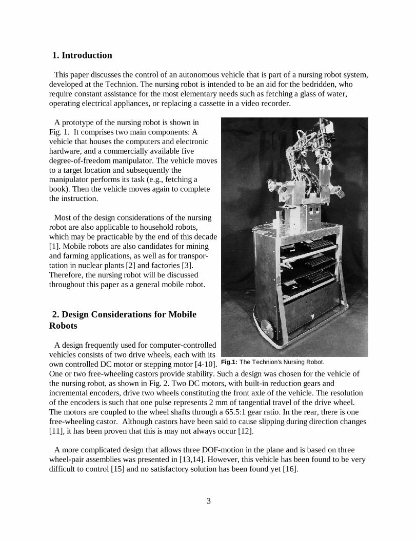
vehicles consists of two drive wheels, each with itsown controlled DC motor or stepping motor [4-10].One or two free-wheeling castors provide stability. Such a design was chosen for the vehicle ofthe nursing robot, as shown in Fig. 2. Two DC motors, with built-in reduction gears andincremental encoders, drive two wheels constituting the front axle of the vehicle. The resolutionof the encoders is such that one pulse represents 2 mm of tangential travel of the drive wheel.The motors are coupled to the wheel shafts through a 65.5:1 gear ratio. In the rear, there is onefree-wheeling castor. Although castors have been said to cause slipping during direction changes[11], it has been proven that this is may not always occur [12].

A more complicated design that allows three DOF-motion in the plane and is based on threewheel-pair assemblies was presented in [13,14]. However, this vehicle has been found to be verydifficult to control [15] and no satisfactory solution has been found yet [16].

��

�x

b

4

Figure 2: Diagram of the mobile platform.

(1)

In mobile robots it is desirable to place the two drive wheels as far apart as possible, for thefollowing reasons:

1. The stability of the vehicle is improved.

2. The effect of the encoder resolution on the orientation error of the vehicle is decreased. Inthe worst case, the orientation error �� is given approximately by

As seen from Eq. (1), the orientation error �� is reduced by increasing the distancebetween the drive wheels (b).

3. During straight-line motion, mechanical disturbances might cause the motors to runtemporarily at different angular speeds, resulting in a temporarily curved path. It can beshown by trigonometry that the radius of the curved path is directly proportional to thewheel separation distance b.

4. Differences in the two wheel diameters will also cause a curved path with a radiusproportional to the distance b.

On the other hand, an exaggerated base width will adversely affect the mobility within a room.In the present design the distance between the two drive wheels is 600 mm.

The position and the orientation of the mobile nursing robot in a room is determined by twoalternate sensing methods; incremental and absolute. When the vehicle is in motion, its positionis measured by the incremental encoders attached to the wheels. The incremental position is

5

accumulated by the control computer, which in turn determines the position and the orientationof the robot in the room. When the vehicle is at rest, an absolute position measuring system isemployed to compensate for the inaccuracies of the incremental method. It comprises three lightsources attached to the room's walls and a rotating light-detecting sensor located on the first jointof the robot. This approach periodically updates the absolute position and orientation of thevehicle, and therefor requires the vehicle's position accuracy while traveling to be relatively high(e.g., a deviation of 1 cm for 1 m traveling distance). Therefore, the avoidance of wheel slippageis extremely important.

Wheel slippage occurs mainly during two types of motions: (a) acceleration and deceleration,and (b) during non-straight-line motions where centrifugal forces cause lateral slippage. Thelatter effect is minimized by limiting non-straight-line motions to "on-the-spot" rotation, whereboth drive wheels run at the same speed but in opposed directions. In this case, and withsymmetric weight distribution, no lateral forces occur at the wheels. Slippage during theacceleration and deceleration phases is reduced by employing low acceleration and decelerationrates (the maximum speed is 0.27 m/s). Another approach to minimize the effect of slippage is to mount the encoders on two additional

freely rotating wheels driven by the vehicle's motion. By dividing the tasks of driving the vehicleand providing feedback information between two sets of wheels, each wheel set may beappropriately designed for its task. The additional wheels were not included in our vehicle, sincethe experimental results obtained with the encoders mounted directly on the drive wheels aresatisfactory for the nursing robot purposes. However, for applications in which more accuratepositioning of the vehicle is required, the two feedback wheels should be added.

3. Motion Control

Motion control means the strategy by which the vehicle approaches a desired location and theimplementation of this strategy.

Motion Types

The nursing robot vehicle is designed to perform only two distinct kinds of motion: straight-linemotion, where both motors are running at the same speed and in the same direction, and rotationabout the vehicle's center-point, where both motors are running at the same speed but in oppositedirections. This approach is advantageous for several reasons:

1. Wheel slippage is minimized because of the simultaneous action or rest of both wheels andbecause of the "on-the-spot" rotation action for turns.

2. A relatively simple control system may be used, since in either case the only task of thecontroller is to maintain equal angular velocities,

1 arctanyfy0

xfx0

L (xfx0)2� (yfy0)

2

6

Fig.3: Procedure for traveling to a new location.

(2)

(3)

3. The vehicle path is always predictable, unlike other motion strategies which smooth sharpcorners by an unpredictably curved path (e.g., [17]). A predictable path is advantageouswhen global path planning, to avoid obstacles, is employed.

4. The vehicle always travels through the shortest possible distance (straight-line or "on-the-spot" rotation).

The Control Algorithm

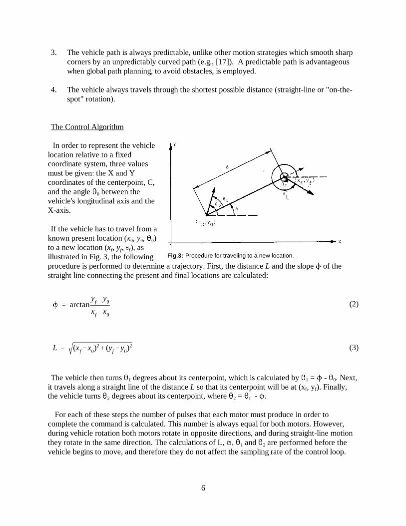
In order to represent the vehiclelocation relative to a fixedcoordinate system, three valuesmust be given: the X and Ycoordinates of the centerpoint, C,and the angle � between the0

vehicle's longitudinal axis and theX-axis.

If the vehicle has to travel from aknown present location (x , y , � )0 0 0

to a new location (x , y , � ), asf f f

illustrated in Fig. 3, the followingprocedure is performed to determine a trajectory. First, the distance L and the slope 1 of thestraight line connecting the present and final locations are calculated:

The vehicle then turns � degrees about its centerpoint, which is calculated by � = 1 - � . Next,1 1 0

it travels along a straight line of the distance L so that its centerpoint will be at (x , y ). Finally,f f

the vehicle turns � degrees about its centerpoint, where � = � - 1.2 2 f

For each of these steps the number of pulses that each motor must produce in order tocomplete the command is calculated. This number is always equal for both motors. However,during vehicle rotation both motors rotate in opposite directions, and during straight-line motionthey rotate in the same direction. The calculations of L, 1, � and � are performed before the1 2

vehicle begins to move, and therefore they do not affect the sampling rate of the control loop.

7

4. Control System Analysis

A conventional controller for a mobile robot consists of two independent control loops, one foreach motor. A similar approach is sometimes used to drive the worktable of CNC millingmachines or Cartesian robots [18,19]. Motion coordination in these systems is achieved byadjusting the reference velocities of the control loops, but the loop of one axis receives noinformation regarding the other. Any load disturbance in one of the axes causes an error that iscorrected only by its own loop, while the other loop carries on as before. This lack ofcoordination causes an error in the resultant path. An improvement in the path accuracy can beachieved by providing cross-coupling, whereby an error in either axis affects the control loops ofboth axes. A cross-coupling method was applied to a Japanese mobile robot [20], in which eachloop used the position error of the other loop, but a signal proportional to the resultant path errorwas not generated. A control analysis is not provided in [20] and experimental results are notreported.

The controller used here, applies an approach similar to the cross-coupled controller, which hasbeen found to be advantageous for two-axis NC and CNC systems [21]. In this design the patherror is calculated and fed as a correction signal to both loops. The main differences between thepresent design and the one used in CNC systems are that here the absolute reference velocities toboth axes are always equal and the controller always maintains the maximum allowable speed ofthe motors, thus enabling the use of smaller motors since they are utilized at their maximum per-formance level.

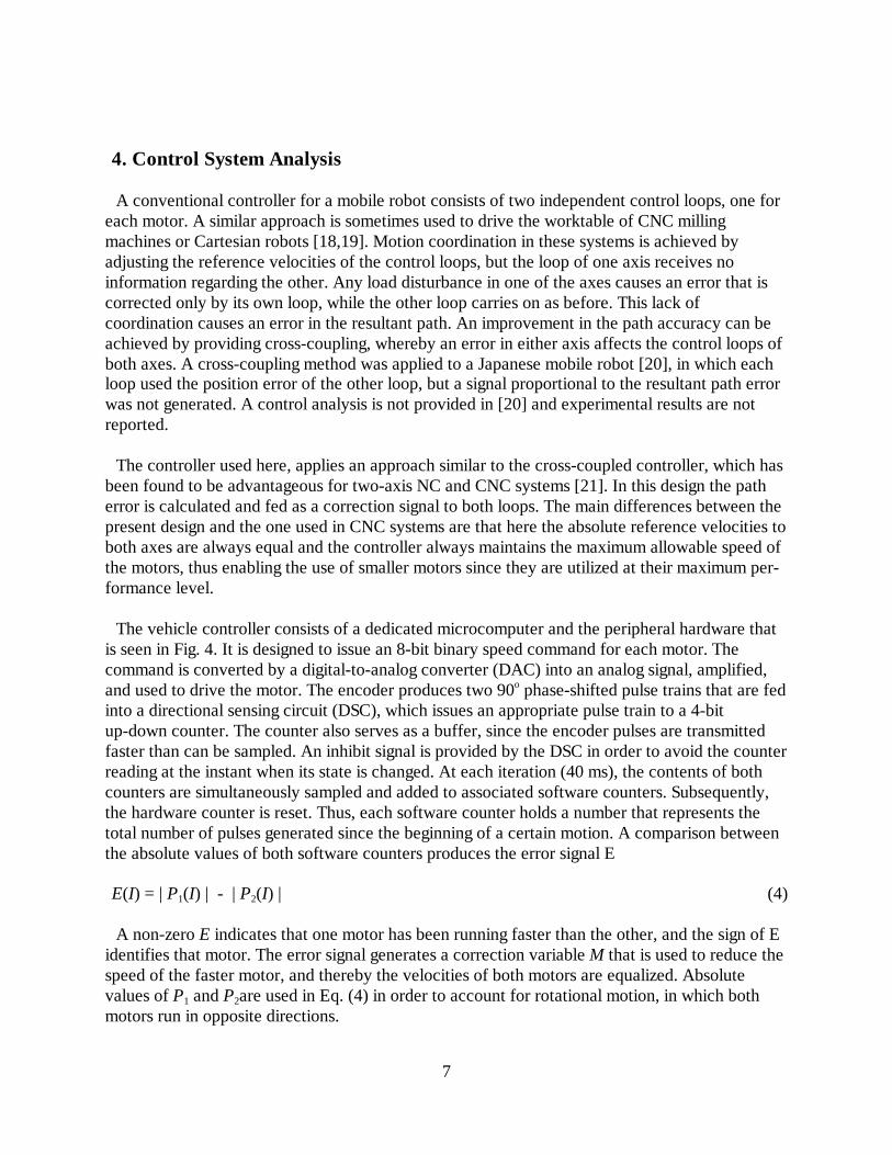
The vehicle controller consists of a dedicated microcomputer and the peripheral hardware thatis seen in Fig. 4. It is designed to issue an 8-bit binary speed command for each motor. Thecommand is converted by a digital-to-analog converter (DAC) into an analog signal, amplified,and used to drive the motor. The encoder produces two 90 phase-shifted pulse trains that are fedo

into a directional sensing circuit (DSC), which issues an appropriate pulse train to a 4-bitup-down counter. The counter also serves as a buffer, since the encoder pulses are transmittedfaster than can be sampled. An inhibit signal is provided by the DSC in order to avoid the counterreading at the instant when its state is changed. At each iteration (40 ms), the contents of bothcounters are simultaneously sampled and added to associated software counters. Subsequently,the hardware counter is reset. Thus, each software counter holds a number that represents thetotal number of pulses generated since the beginning of a certain motion. A comparison betweenthe absolute values of both software counters produces the error signal E

E(I) = | P (I) | - | P (I) | (4)1 2

A non-zero E indicates that one motor has been running faster than the other, and the sign of Eidentifies that motor. The error signal generates a correction variable M that is used to reduce thespeed of the faster motor, and thereby the velocities of both motors are equalized. Absolutevalues of P and P are used in Eq. (4) in order to account for rotational motion, in which both1 2

motors run in opposite directions.

8

Figure. 4 : The control loops of the mobile platform.

Any temporary disturbance of the steady-state velocities will be successfully corrected by aproportional (P) controller. However, in order to correct a continuous disturbance, as might becaused by different friction forces in the bearings (e.g., due to an asymmetric load distribution onthe vehicle), an integral (I) action is required as well. The PI-controller provides not only equalvelocities but also an equal overall pulse count from the beginning of each motion. Therefore, thiscontroller guarantees a zero steady-state orientation error of the vehicle for any constantcontinuous disturbance (except for slippage).

The equations of the PI-controller are

S(I) = S(I-1) + E(I) (5)

M(I) = K S(I) + K E(I) (6)c p

where K is the integration gain and K is the proportional gain. The ranges of K and K thatc p c p

guarantee stability of the system have been determined as described in the following table:

H = 3 pulses/rev K = 0.02 volt/pulse a

K = 18.4 rev/voltb

K = 1 secc-1

K = 12p

T = 0.04 sec= 1.0 volt/Nm= 0.2 sec

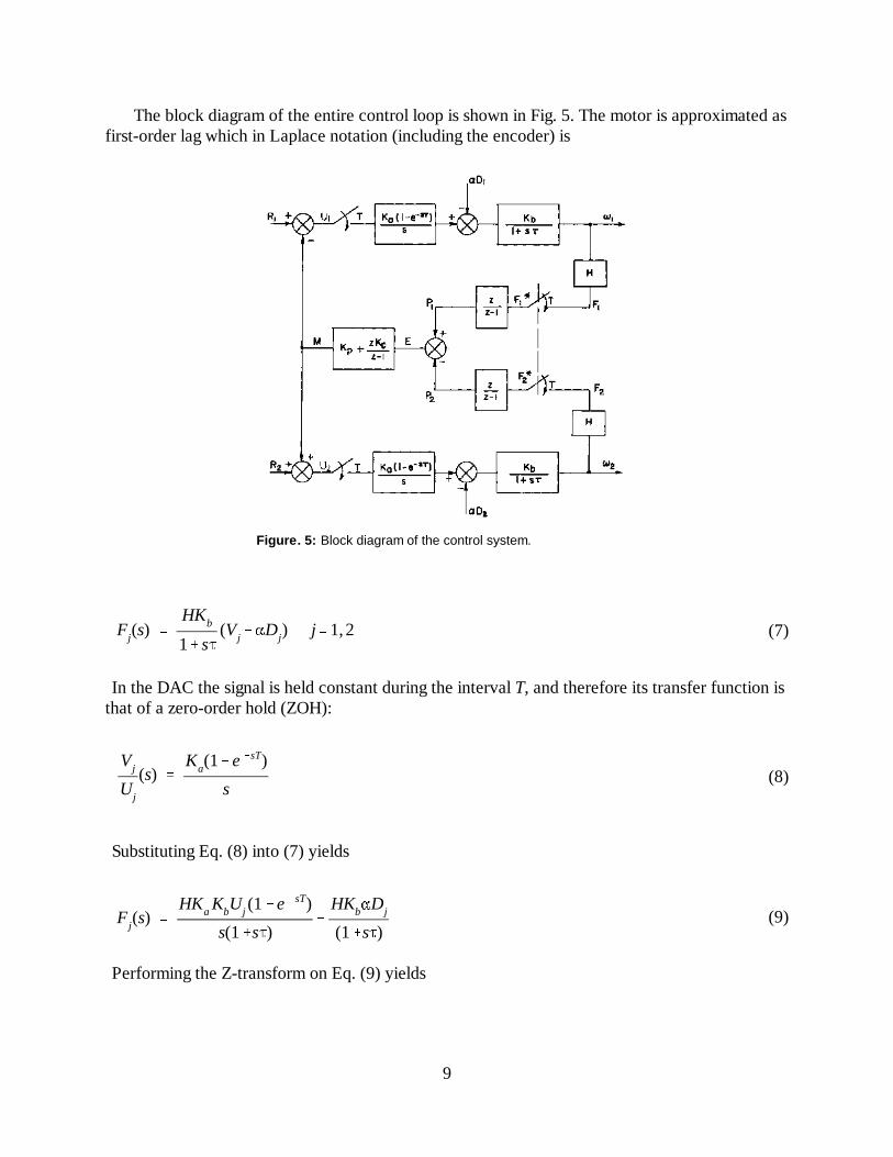
Fj(s) HKb

1�s-(Vj�Dj) j1,2

Vj

Uj

(s) Ka(1esT)

s

Fj(s) HKaKbUj (1esT)

s(1�s-)

HKb�Dj

(1�s-)

9

Figure. 5: Block diagram of the control system.

(7)

(8)

(9)

The block diagram of the entire control loop is shown in Fig. 5. The motor is approximated asfirst-order lag which in Laplace notation (including the encoder) is

In the DAC the signal is held constant during the interval T, and therefore its transfer function isthat of a zero-order hold (ZOH):

Substituting Eq. (8) into (7) yields

Performing the Z-transform on Eq. (9) yields

Fj(z) K (1r)

(zr)U

j(z) HK

b

z7(zr)

�Dj(z)

r exp(T-

) exp(0.040.2

) 0.82

7

1- 5s1

Pj(z) z

z1Fj(z) j 1,2

E(z) P1(z)P2(z) z

z1(F1(z)F2(z))

M(z) (Kp�Kc

zz1

)E(z)

F1(z) K(1rzr

) [R1(z)��(Kp�Kc

zz1

)E(z)] HKb(z7zr

)�D1(z)

10

(10)

(11)

(12)

(13)

(15a)

where K is the open-loop gain given by K = K K H = 0.02 # 18.4 # 3 = 1.1 pulses/(s # volt) and ra b

and 7 are defines as

The software control algorithm may be represented with the aid of the Z-transform as

U (z) = R (z) + � M(z) (14a)1 1 1

U (z) = R (z) + � M(z) (14b)2 2 2

where � = 0 and � = 1, for negative M1 2

and � = 1 and � = 0, for positive M1 2

Substituting Eqs. (13) and (14) into Eq. (10) gives

F2(z) K( 1rzr

) [R2(z)��(Kp�Kc

zz1

)E(z)] HKb( z7zr

)�D2(z)

F1(z)F2(z) K( 1rzr

)(Kp�Kc

zz1

)E(z) � HKb( z7zr

)�D(z)

E(z) z

z1[K(

1rzr

)(Kp�Kc

zz1

)E(z) � HKb(

z7zr

)�D(z)]

E(z)�D(z)

z2(z1)HKb7

(z1)2 (zr)�z(z1)KKp(1r)�z2KKc

(1r)

Q(z) z3� [K(1r)(Kp�Kc

) (2�r)]z2� [1�2r K(1r)Kp

]z r

Q(z) a3z3�a2z

2� a1z a0

11

(15b)

(16)

(17)

(18)

(19)

(20)

For straight-line motion R = R and therefore the difference between these two signals is1 2

where

�D(z) = �D (z) - �D (z)2 1

Substituting Eq. (16) into Eq. (12) gives the solution of E(z)

The corresponding transfer function is

with the characteristic equation

We define

wherea = 13

a = K(1-r)(K + K ) - (2+r)2 p c

a = 1 + 2r - K K (1-r)1 p

a = -r0

Jury's stability criterion [22] requires that the following four conditions are satisfied:

Kc <4(1�r)

K(1r) 2Kp

b0

a0 a3

a3 a0

b2

a0 a1

a3 a2

Kc > Kp(1

r1)

2(1r 2)

K(1r)r

12

(24a)

(28a)

1. Q(z=1) > 0 (21)

This condition yields

K > 0 (22)c

2. Q(z=-1) < 0 (23)

which gives

or, by substituting the values for K and r

K < 36 - 2K (24b)c p

3. | a | < a (25)0 3

This condition is always satisfied and adds no information.

4. | b | > b (26)0 2

where

namely

1-r > | -(1-r ) + K(1-r) K - K(1-r)rK | (27)2 2 2p c

Equation (27) contains two cases:

a. b < 1 - r22

which yields

Kc < Kp(1

r1)

13

(29a)

Figure. 6: Allowable range for the gains K and K , with experimentalp c

results. (+ = stable, - = unstable)

and after substitution of K and r

K > 0.22K - 4 (28b)c p

b. b > -(1-r )22

which yields

and by substituting r

K < 0.22K (29b)c p

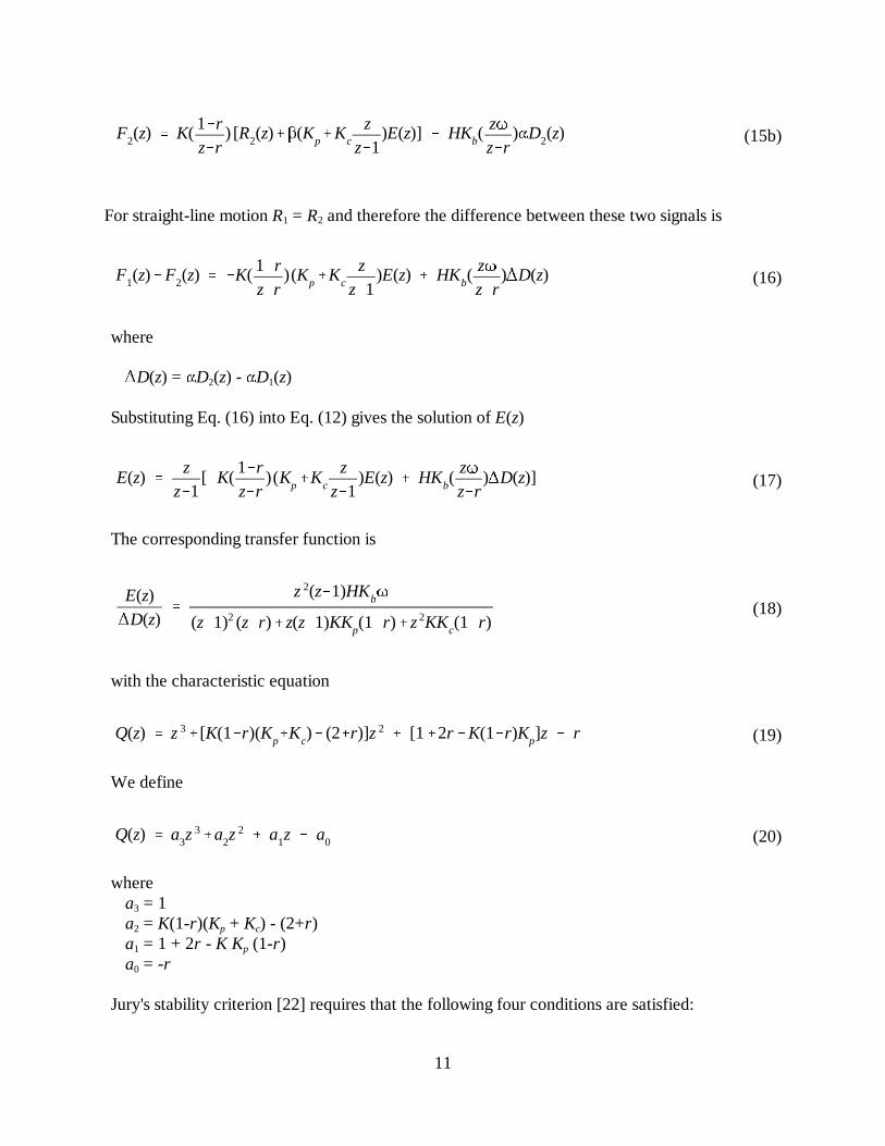
The three inequalities (22), (24), and (29) define a range in the K - K plane in which stability isc p

guaranteed. in order to verify the analysis, the prototype vehicle was tested with several gainvalues. The results (stable = '+', unstable = '-') have been plotted in Fig. 6, and most of them fitthe theoretical analysis. Figure 7 shows typical experimental results of the error E as a responseto a step input in the Disturbance D for K = 12 and three K gain values. For K = 3 the system isp c c

unstable. it is undesirable to select gains that are too close to the boundaries in Fig. 6 (e.g., theleft zone in which K < 9 or the upper zone in which K > 2). We selected the values K = 12 andp c p

K = 1 for the nursing robot vehicle.c

in order to show that the steady state orientation error E' due to a continuous disturbance �Dss 0

is zero, one must recall that the orientation error E' is directly proportional to the differencebetween the accumulated pulse counts of both motors, such that

E' = c(P - P ) = cE (30)1 2

Substituting the difference in disturbing torques

�D(z) zz1

�D0

E �(z) c

z2(z1)HKb7z

z1�D0

(z1)2(zr)�z(z1)KKp(1r)�z2KKc(1r)

14

(31)

(32)

Figure. 7: Experimental response to a stepdisturbance with K =12 and p

a) K = 1 b) K = 2 c) K = 3c c c

and Eq. (18) into Eq. (31) yields

Applying the final value theorem shows that thesteady-state orientation error is zero:

E' = lim (z-1)E'(z) = 0 (33)ss z�1

as was claimed above.

5. Experimental Results

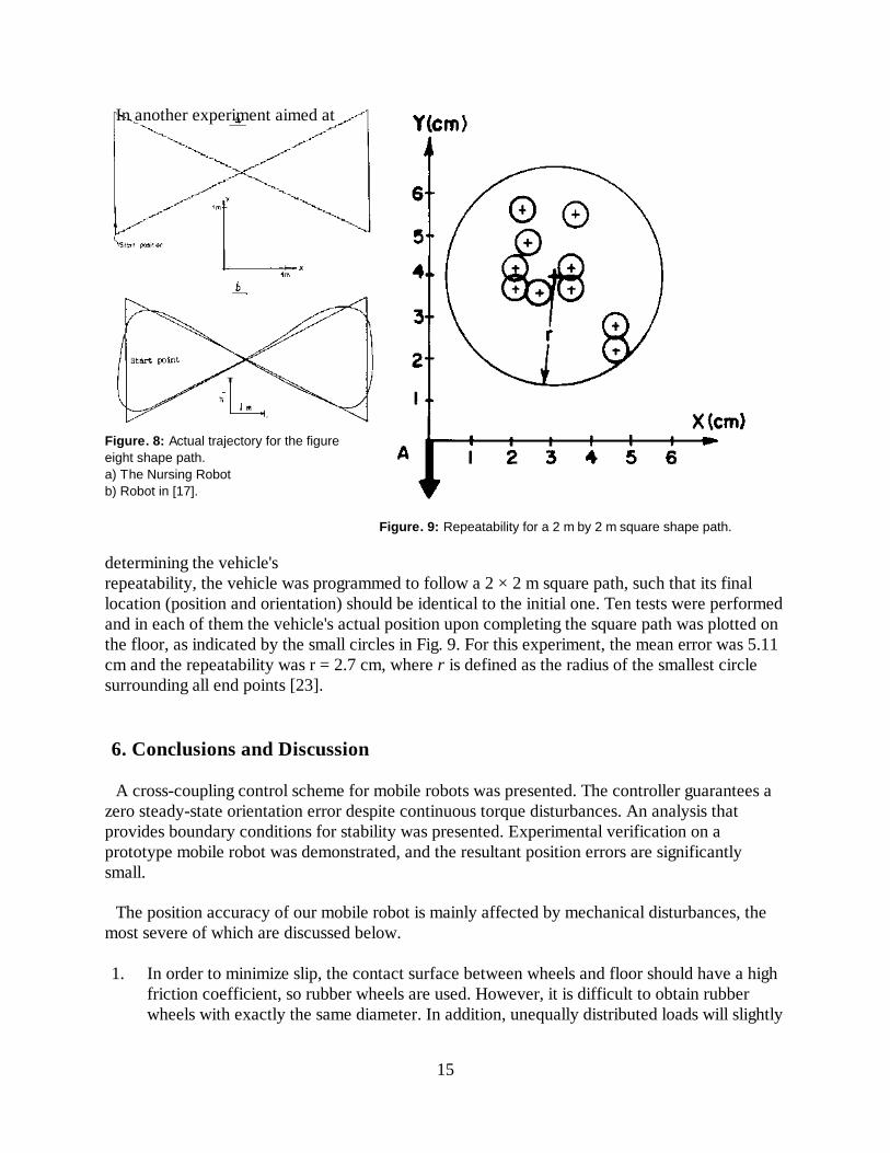
The vehicle shown in Fig. 1 was tested. Experimentshave shown that the position errors recorded by thecontrol system are very small, on the order ofmagnitude of 10 mm per 10 m straight travel [12].

In one test the vehicle was programmed to travel alonga figure-eight path with an overall length of about 13m. The path, as recorded by the control system, isshown in Fig. 8a. After returning to the original startinglocation, the vehicle's calculated path position error (E)was less than 10 mm lateral and less than 1( rotational.This error does not include mechanically inducedaccuracies. The real position error, includingmechanical inaccuracies and actually measured on thefloor (external to the robot), was 6 cm lateral and 1(rotational. These results compare favorably to theresults of a similar experiment described in [17]. A plotof one of the results in [17] has been reproduced here (Fig. 8b) for comparison. However, thevehicle used in [17] was faster, heavier, and did not halt at the corners of the programmed path.

15

Figure. 8: Actual trajectory for the figureeight shape path.a) The Nursing Robot b) Robot in [17].

Figure. 9: Repeatability for a 2 m by 2 m square shape path.

In another experiment aimed at

determining the vehicle'srepeatability, the vehicle was programmed to follow a 2 × 2 m square path, such that its finallocation (position and orientation) should be identical to the initial one. Ten tests were performedand in each of them the vehicle's actual position upon completing the square path was plotted onthe floor, as indicated by the small circles in Fig. 9. For this experiment, the mean error was 5.11cm and the repeatability was r = 2.7 cm, where r is defined as the radius of the smallest circlesurrounding all end points [23].

6. Conclusions and Discussion

A cross-coupling control scheme for mobile robots was presented. The controller guarantees azero steady-state orientation error despite continuous torque disturbances. An analysis thatprovides boundary conditions for stability was presented. Experimental verification on aprototype mobile robot was demonstrated, and the resultant position errors are significantlysmall.

The position accuracy of our mobile robot is mainly affected by mechanical disturbances, themost severe of which are discussed below.

1. In order to minimize slip, the contact surface between wheels and floor should have a highfriction coefficient, so rubber wheels are used. However, it is difficult to obtain rubberwheels with exactly the same diameter. In addition, unequally distributed loads will slightly

16

compress one wheel more than the other, thus changing its rolling radius. Wheels withdifferent diameters cause the vehicle to travel along an arc, rather than along a straightline, even if the motors are running at equal speeds. A rigid wheel design [7] is thereforepreferable. In our vehicle, accurately milled wheels with a 2-mm coating ("tire") wereutilized.

2. There is a contact area, rather than a contact point, between the wheel and the floor. Thiscauses an uncertainty about the effective distance between the drive wheels, creatinginaccuracies when turning.

3. Another major mechanical disturbance is caused by the misalignment of the drive wheels.This effect will produce a lateral drag force resulting in a curved path even when bothwheels are exactly of the same diameter and are rotating at the same angular velocity.Although it is difficult to analytically calculate the magnitude of this disturbance, it can beeasily determined experimentally. This disturbance, along with the one mentioned in item1, can be compensated for by employing a correction factor in the controller algorithm.The correction factor multiplies the number of pulses arriving from one wheel. In our casethe vehicle path, when loaded symmetrically, was always slightly curved to the left. There-fore, the number of pulses sampled from the left wheel is multiplied by 0.992, anexperimentally determined correction factor. This correction factor causes the controller toslightly increase the left wheel speed (here by about 0.8%). In our experiments, thismeasure was found to substantially increase the vehicle's absolute position accuracy.

Finally, it is worthwhile to note that the nursing robot employs a system of navigation beaconsin order to periodically update the vehicle's absolute position. Because of the high accuracy ofthe vehicle, the absolute updating is necessary only at the beginning and at the end of a specifictask, namely, when the vehicle is at rest awaiting a new task.

References

(1) Koren, Y., Robotics for Engineers, McGraw-Hill Book Co. New-York, 1985. pp. 8-10.

(2) Weisbin, C., Saussure G., and Kammer, D.: "Self-Controlled, a Real-Time Expert System forAutonomous Mobile Robot," Computers in Mechanical Eng.. Sept. 1986, pp.12-19.

(3) Dorf R. C., Robotics and Automated Manufacturing, Prentice-Hall Co., Reston, 1983.

(4) Bauzil, G., Briot, M., and Ribes, P., "A Navigation Sub-System Using Ultrasonic Sensors for theMobile Robot HILARE," 1st Int. Conf. on Robot Vision and Sensory Controls, Stratford-upon-Avon, UK.,April 1981, pp. 47-58.

(5) Julliere, M., Marce, L., and Place, H., "A Guidance System for a Mobile Robot," Proc. of the 13th Int.Symp. on Industrial Robots and Robots, Chicago, Ill., April, 1983, pp. 13.58-13.68.

(6) Cooke, R.A., "Microcomputer Control of Free Ranging Robots," Proc. of the 13th Int. Symp. onIndustrial Robots and Robots, Chicago, Ill., April 1983, pp. 13.109-13.120.

17

(7) Iijima, J., Yuta, S., and Kanayama, Y., "Elementary Functions of a Self-Contained Robot'YAMABICO 3.1'," Proc. of the 11th Int. Symp. on Industrial Robots, Tokyo 1983, pp. 211-218.

(8) Fujiwara, K. and al., "Development of Guideless Robot Vehicle," Proc. of the 11th Int. Symp. onIndustrial Robots, Tokyo 1983, pp 203-210.

(9) Nakamura, T., "Edge Distribution Understanding For Locating a Mobile Robot," Proc. of the 11th Int.Symp. on Industrial Robots, Tokyo 1981, pp. 195-202.

(10) Hollis, R., "NEWT, A Mobile, Cognitive Robot," BYTE, June 1977, pp. 30-45.

(11) Carlisle, B., "An Omni-Directional Mobile Robot," Developments in Robotics 1983, IFSPublications, Kempston, England 1983. (12) Borenstein, J. and Koren, Y., "A Mobile Platform For Nursing Robots," IEEE Transactions on

Industrial Electronics, June 1985.

(13) Moravec, H. P., "The CMU Rover," Proceedings of the National Conference of ArtificialIntelligence, AAAI-82, August 1982, pp. 377-380.

(14) Moravec, H. P., "The Stanford Cart and the CMU Rover," Proceedings of the IEEE, Vol. 71, No 7,July 1983. pp. 872-884.

(15) Moravec, H. P., "Robots That Rove," Internal Report of the Robotics Institute, Carnegie-MellonUniversity.

(16) Moravec, H. P., "Three Degrees for a Mobile Robot," Internal Report of the Robotics Institute,Carnegie-Mellon University, July 1984.

(17) Tsumura, T., Fujiwara, N., Shirakawa, T., and Hashimoto, M., "An Experimental System forAutomatic Guidance of Roboted Vehicle Following the Route Stored in Memory," Proc. of the 11th Int.Symp. on Industrial Robots, Tokyo 1981, pp. 187-193.

(18) Koren, Y., Computer Control of Manufacturing Systems, McGraw-Hill Book Co., New York 1983.

(19) Koren, Y., "Control of Machine Tools and Robots," Applied Mechanics Reviews, Vol. 39, No. 9,Sept. 1986, pp. 1331-1338.

(20) Fujii, S. et al., "Computer Control of a Locomotive Robot with Visual Feedback," Proc. of the 11thInt. Symp. on Industrial Robots, Tokyo 1981, pp. 219-226.

(21) Koren, Y., "Cross-Coupled Biaxial Computer Control for Manufacturing Systems," Transactions ofthe ASME, Journal of Dynamic Systems, Measurement and Control, Vol. 102, December 1980, pp.265-272.

(22) Kuo, B. C., Analysis and Synthesis of Sampled-Data Control Systems, Prentice-Hall, Inc.,Englewood Cliffs, N. J., 1983.

(23) Alberson, P., "Verifying Robot Performance," Robotics Today, Oct. 1983, pp. 33-36.