radio telescope antenna azimuth position control system design and

BULETINUL INSTITUTULUI POLITEHNIC DIN IAŞI

Publicat de

Universitatea Tehnică „Gheorghe Asachi” din Iaşi

Tomul LX (LXIV), Fasc. 3-4, 2014

Secţia

AUTOMATICĂ şi CALCULATOARE

RADIO TELESCOPE ANTENNA AZIMUTH POSITION

CONTROL SYSTEM DESIGN AND ANALYSIS IN

MATLAB/SIMULINK USING PID & LQR CONTROLLER

BY

ABDUL REHMAN CHISHTI1, SYED FASIH-UR-REHMAN BUKHARI2,

HAFIZ SAAD KHALIQ1, MOHAMMAD HUNAIN KHAN1

and SYED ZULFIQAR HAIDER BUKHARI1

The Islamia University of Bahawalpur, Pakistan,

1Dept. of Telecom Engineering, University College of Engineering & Technology 2Dept. of Electronics Engineering, University College of Engineering & Technology

Received: September 12, 2014

Accepted for publication: November 5, 2014

Abstract. A position control system converts an input position command to an

output position response. Antennas, computer disk drives and robot arms contains

many applications of position control system. The radio telescope antenna utilizes

position control systems. In this paper the design and control of antenna azimuth

position has been implemented. The response of the system is analysed and results

are drawn by using PID controller, the results of PID controller are further

improved by adding Linear Quadratic Regulator. We have seen that the LQR

results are much better than the results obtained by PID controller.

Key words: LQR; PID controller; system response; azimuth position control;

MATLAB simulation.

2010 Mathematics Subject Classification: 93C83, 34C60.

Corresponding author; e-mail: [email protected]

46 Abdul Rehman Chishti et al.

1. Introduction

Currently the modern world depends on control systems. Various

applications in our surrounding use the concepts of control systems. Such

applications include the automatic lifts, robotics, the rocket fire and the space

shuttle lifts of to earth, car’s hydraulic pistons and many other real life

applications. Our body organs as pancreas which regulates our blood sugar,

heart which pumps through all parts of our body and brain which controls

electric pulses through our backbone etc. all are natural control systems. So

control systems have lot of applications in our life, we are surrounded by

modern technologies which based on scientific innovations. One would have

heard about an aircraft flying in auto mode, a moving vehicle without operator

and an antenna which gives maximum auto signal strength all are the

applications of control systems.

Control system is a system designed for obtaining required

characteristics of a process. For getting desired yield with desired performance

many subsystems and processes linked in a control system (Nise, 2000). An

example of control system is shown in Fig. 1.

Fig. 1 – Control System.

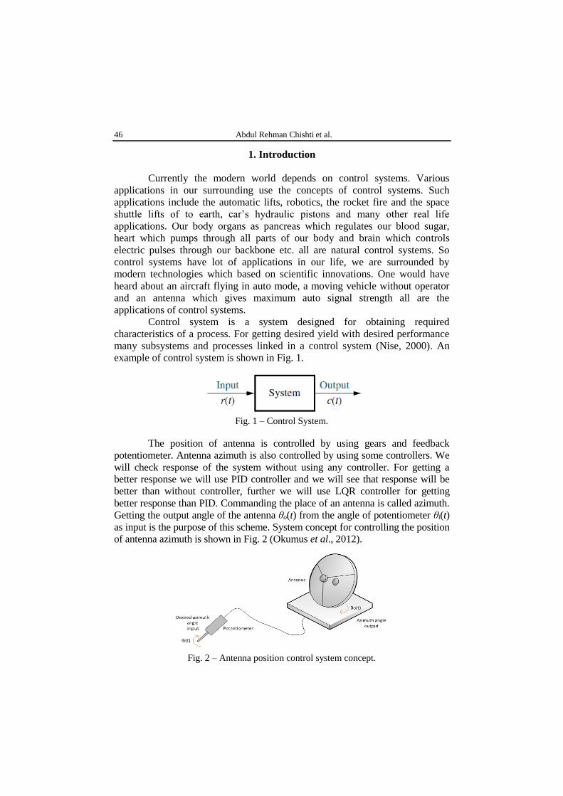
The position of antenna is controlled by using gears and feedback

potentiometer. Antenna azimuth is also controlled by using some controllers. We

will check response of the system without using any controller. For getting a

better response we will use PID controller and we will see that response will be

better than without controller, further we will use LQR controller for getting

better response than PID. Commanding the place of an antenna is called azimuth.

Getting the output angle of the antenna θo(t) from the angle of potentiometer θi(t)

as input is the purpose of this scheme. System concept for controlling the position

of antenna azimuth is shown in Fig. 2 (Okumus et al., 2012).

Fig. 2 – Antenna position control system concept.

Bul. Inst. Polit. Iaşi, t. LX (LXIV), f. 3-4, 2014

47

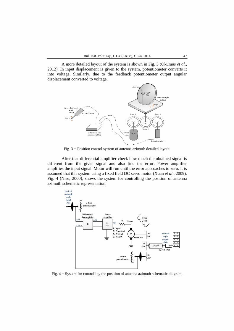
A more detailed layout of the system is shown in Fig. 3 (Okumus et al.,

2012). In input displacement is given to the system, potentiometer converts it

into voltage. Similarly, due to the feedback potentiometer output angular

displacement converted to voltage.

Fig. 3 − Position control system of antenna azimuth detailed layout.

After that differential amplifier check how much the obtained signal is

different from the given signal and also find the error. Power amplifier

amplifies the input signal. Motor will run until the error approaches to zero. It is

assumed that this system using a fixed field DC servo motor (Xuan et al., 2009).

Fig. 4 (Nise, 2000), shows the system for controlling the position of antenna

azimuth schematic representation.

Fig. 4 − System for controlling the position of antenna azimuth schematic diagram.


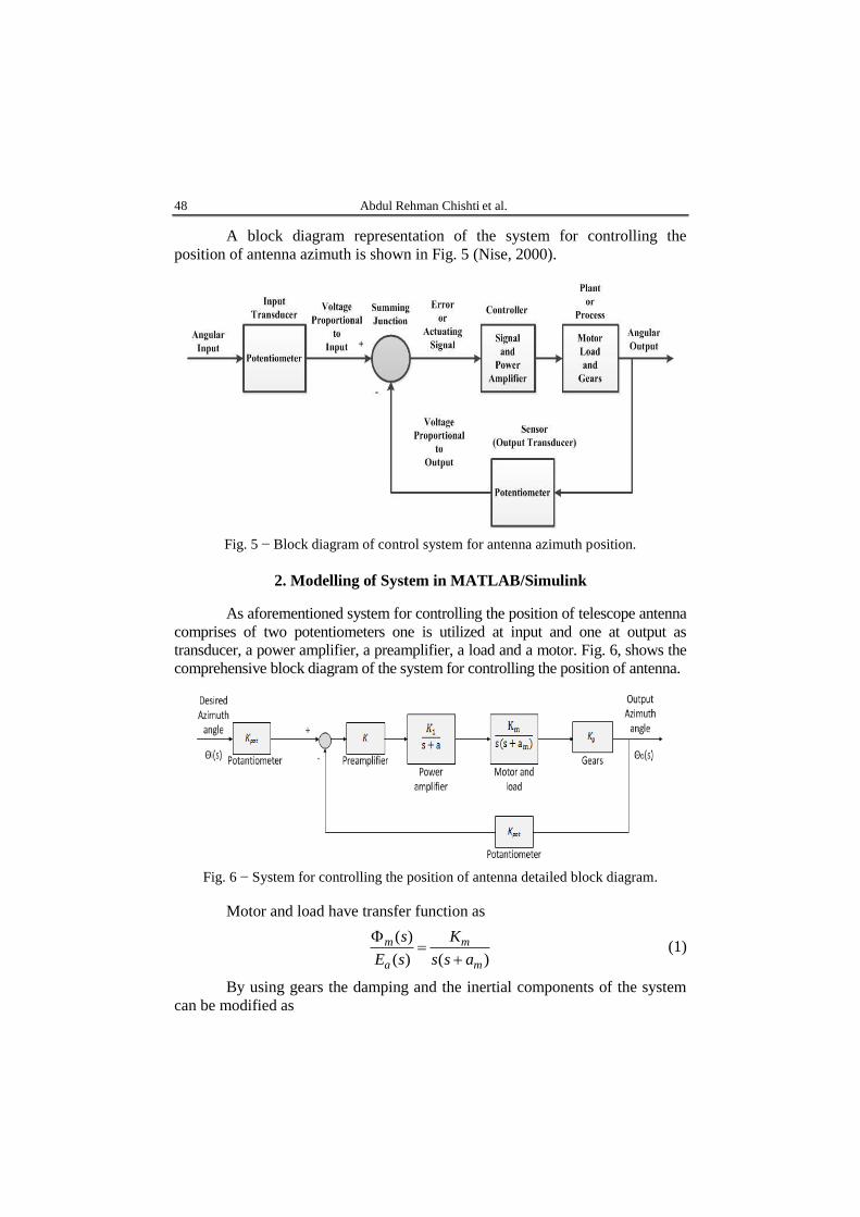
A block diagram representation of the system for controlling the

position of antenna azimuth is shown in Fig. 5 (Nise, 2000).

Fig. 5 − Block diagram of control system for antenna azimuth position.

2. Modelling of System in MATLAB/Simulink

As aforementioned system for controlling the position of telescope antenna

comprises of two potentiometers one is utilized at input and one at output as

transducer, a power amplifier, a preamplifier, a load and a motor. Fig. 6, shows the

comprehensive block diagram of the system for controlling the position of antenna.

Fig. 6 − System for controlling the position of antenna detailed block diagram.

Motor and load have transfer function as

( )

( ) ( )

m m

a m

s K

E s s s a

(1)

By using gears the damping and the inertial components of the system

can be modified as


49

1

2

250.1

250g

NK

N (2)

In the above equation, N1 and N2 represent the gear teeth as shown in

Fig. 3. The calculation of inertial and damping components is given as

2 2( ) 0.02 1(0.1) 0.03a L gJ J J K (3)

2 2( ) 0.01 1(0.1) 0.02m a L gD D D K (4)

Motor and load block’s pole and zero is represented as

(0.02)(8) (0.5)(0.5)

1.71(0.03)(8)

m a b tm

a

D R K Ka

J R

(5)

0.5

2.083(0.03)(8)

tm

a

KK

JR (6)

In the above equations, Ra is the resistance (Ω) of the motor, Kb and Kt

are the back EMF and torque constant of the motor respectively. Parameters for

preamplifier, power amplifier and gears of above block diagram are given in

Table 1.

Table 1 Parameters of Antenna Block Diagram

Parameters Configurations

K ------

Kpot 0.318

a 100

K1 100

Kg 0.1

In Table 1, gain value “K” represents the preamplifier block. The value

of preamplifier gain “K” can be found out for stable system by utilizing the

Routh-Herwitz criterion. According to this this criterion, system will give stable

response if we take the value of gain “K” in the range 0-262.3. Here, the value

of gain taken is 100 which is in the above mentioned range.

The close loop transfer function of system for controlling the position

of antenna azimuth (Nise, 2000) is provided as

3 2

( ) 6.63

( ) 101.71 171 6.63

o

i

s K

s s s s K

(7)

If we use the value of gain “K” as we have find by using Routh-Herwitz

criterion. Then, the equation in (7) can be written as


3 2

( ) 663

( ) 101.71 171 663

o

i

s

s s s s

(8)

Now we can represent the state space of our close loop transfer

function. First time Kalman represent the state space in 1959 (Kalman, 1960)

and this step gives a new concept in world to control the systems and later

concept named as “modern control theory”. State of close loop transfer function

of azimuth position control of antenna is represented as

101.7100 171.0000 663.0000

1.0000 0 0

0 1.0000 0

A

1

0

0

B

0 0 663C

0D

We can find the response of control system of antenna azimuth position

by using close-loop transfer function given in (8). But first we find open loop

response then move towards close loop response. For open loop response of

control system of antenna azimuth position we need a transfer function without

feedback in which we will deal with a power amplifier and a motor with load

which is given as

2

20.83( )

101.71 171G s

s s

(9)

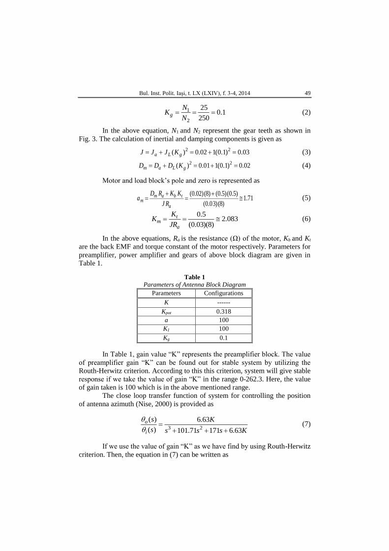
Fig. 7, shows the open loop step and impulse response of the system for

controlling the azimuth position of telescope antenna. We have got an idea that

this resultant response is not good. Open loop response does not give us desired

response. So, for getting desired response we will use close loop system. Close

loop system will provide us a good and stable response.


51

0 0.5 1 1.5 2 2.5 3 3.50

0.02

0.04

0.06

0.08

0.1

0.12

0.14

0.16

0.18

0.2

Step Response

Impulse Response

Responses of Open Loop System

Time (seconds)

Am

plit

ude

Fig. 7 − Open Loop Response.

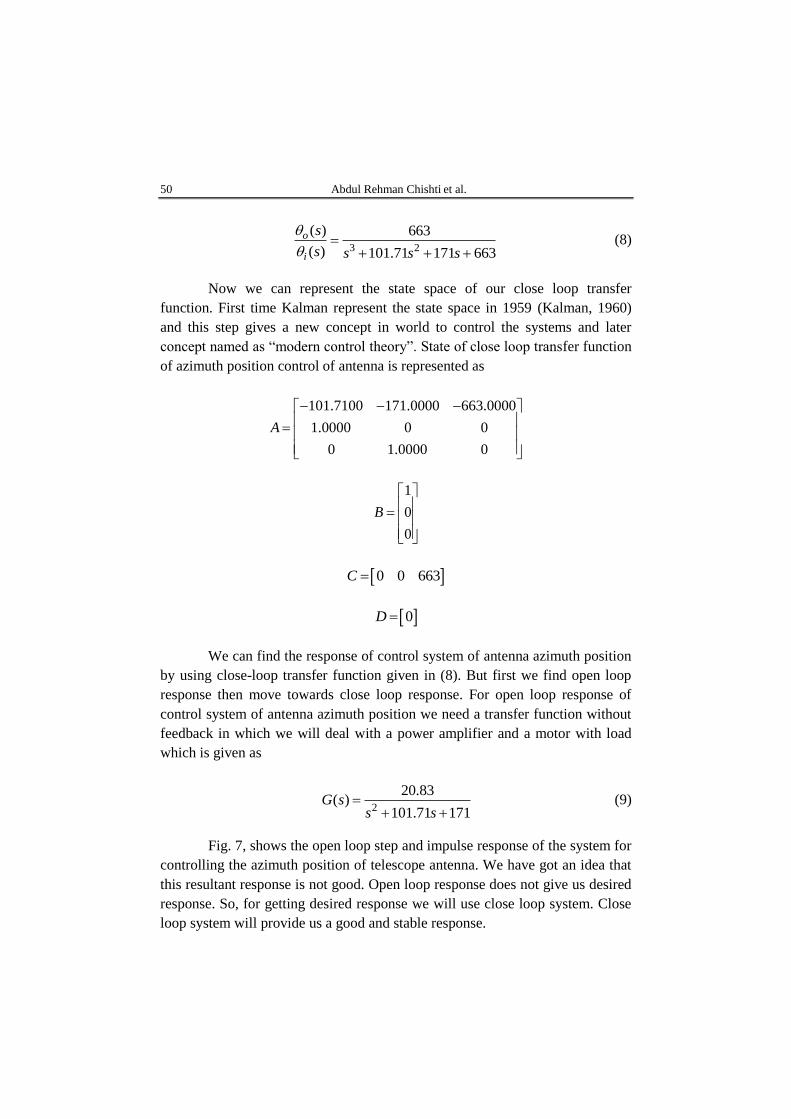
Fig. 8, shows the close loop step and impulse response of the system for

controlling the position of telescope antenna. As we discuss earlier that close

loop system provide us a good response. By comparing with open loop response

we have got an idea that the close loop response is better than open loop but for

our system this response is not good. This response is without any controller.

For getting more stable response we will use a controller in the next section.

0 2 4 6 8 10 12 14 16 18-1.5

-1

-0.5

0

0.5

1

1.5

2

2.5

Step Response

Impulse Response

Step Response

Impulse Response

Step Response

Impulse Response

Step Response

Impulse Response

Step Response

Impulse Response

Step Response

Impulse Response

Response of Close Loop System

Time (seconds)

Am

plit

ude

Fig. 8 − Close Loop Response.


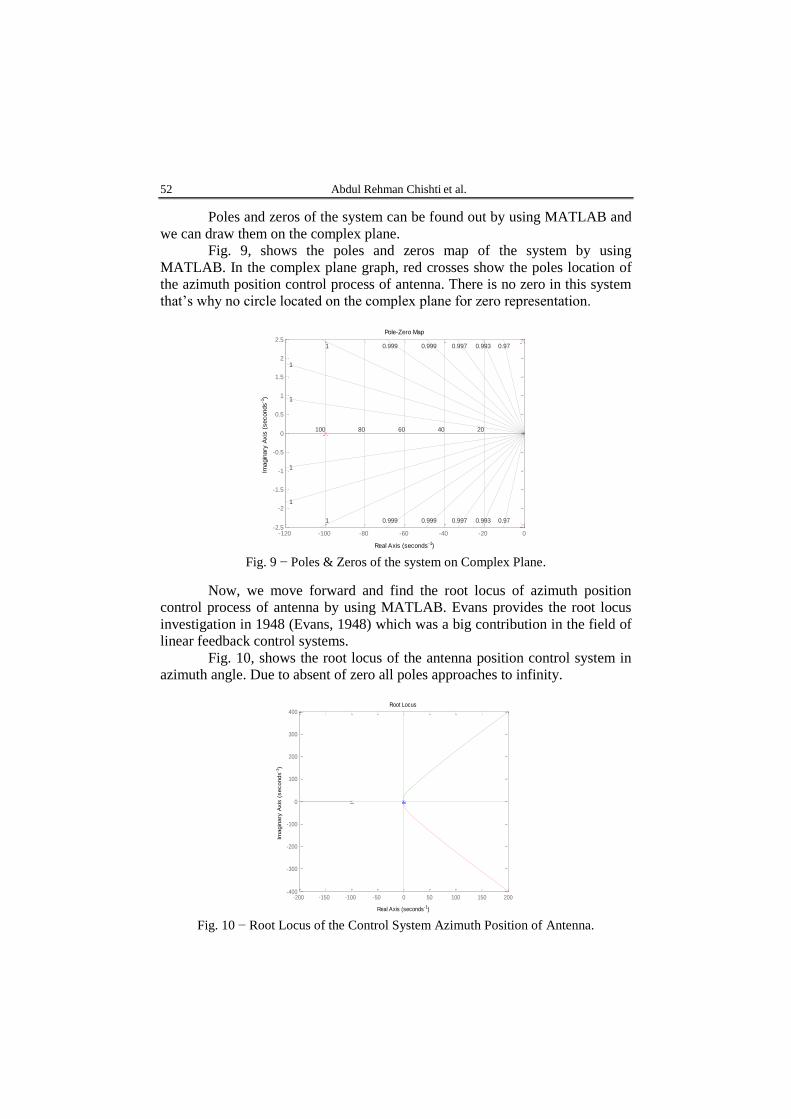
Poles and zeros of the system can be found out by using MATLAB and

we can draw them on the complex plane.

Fig. 9, shows the poles and zeros map of the system by using

MATLAB. In the complex plane graph, red crosses show the poles location of

the azimuth position control process of antenna. There is no zero in this system

that’s why no circle located on the complex plane for zero representation.

-120 -100 -80 -60 -40 -20 0-2.5

-2

-1.5

-1

-0.5

0

0.5

1

1.5

2

2.50.970.9930.9970.9990.9991

1

1

0.970.9930.9970.9990.9991

1

1

20406080100120

Pole-Zero Map

Real Axis (seconds-1)

Imagin

ary

Axis

(seconds

-1)

Fig. 9 − Poles & Zeros of the system on Complex Plane.

Now, we move forward and find the root locus of azimuth position

control process of antenna by using MATLAB. Evans provides the root locus

investigation in 1948 (Evans, 1948) which was a big contribution in the field of

linear feedback control systems.

Fig. 10, shows the root locus of the antenna position control system in

azimuth angle. Due to absent of zero all poles approaches to infinity.

-200 -150 -100 -50 0 50 100 150 200-400

-300

-200

-100

0

100

200

300

400

Root Locus

Real Axis (seconds-1)

Imagin

ary

Axis

(seconds

-1)

Fig. 10 − Root Locus of the Control System Azimuth Position of Antenna.


53

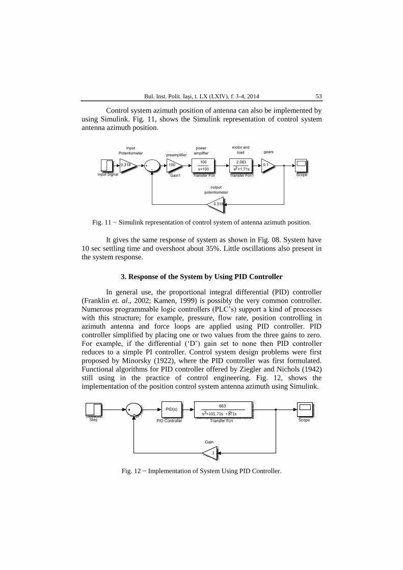
Control system azimuth position of antenna can also be implemented by

using Simulink. Fig. 11, shows the Simulink representation of control system

antenna azimuth position.

Fig. 11 − Simulink representation of control system of antenna azimuth position.

It gives the same response of system as shown in Fig. 08. System have

10 sec settling time and overshoot about 35%. Little oscillations also present in

the system response.

3. Response of the System by Using PID Controller

In general use, the proportional integral differential (PID) controller

(Franklin et. al., 2002; Kamen, 1999) is possibly the very common controller.

Numerous programmable logic controllers (PLC’s) support a kind of processes

with this structure; for example, pressure, flow rate, position controlling in

azimuth antenna and force loops are applied using PID controller. PID

controller simplified by placing one or two values from the three gains to zero.

For example, if the differential (‘D’) gain set to none then PID controller

reduces to a simple PI controller. Control system design problems were first

proposed by Minorsky (1922), where the PID controller was first formulated.

Functional algorithms for PID controller offered by Ziegler and Nichols (1942)

still using in the practice of control engineering. Fig. 12, shows the

implementation of the position control system antenna azimuth using Simulink.

Step

PID(s) PID Controller

663 s +101.71s +171s 3 2

Transfer Fcn

1 Gain

Scope

Fig. 12 − Implementation of System Using PID Controller.


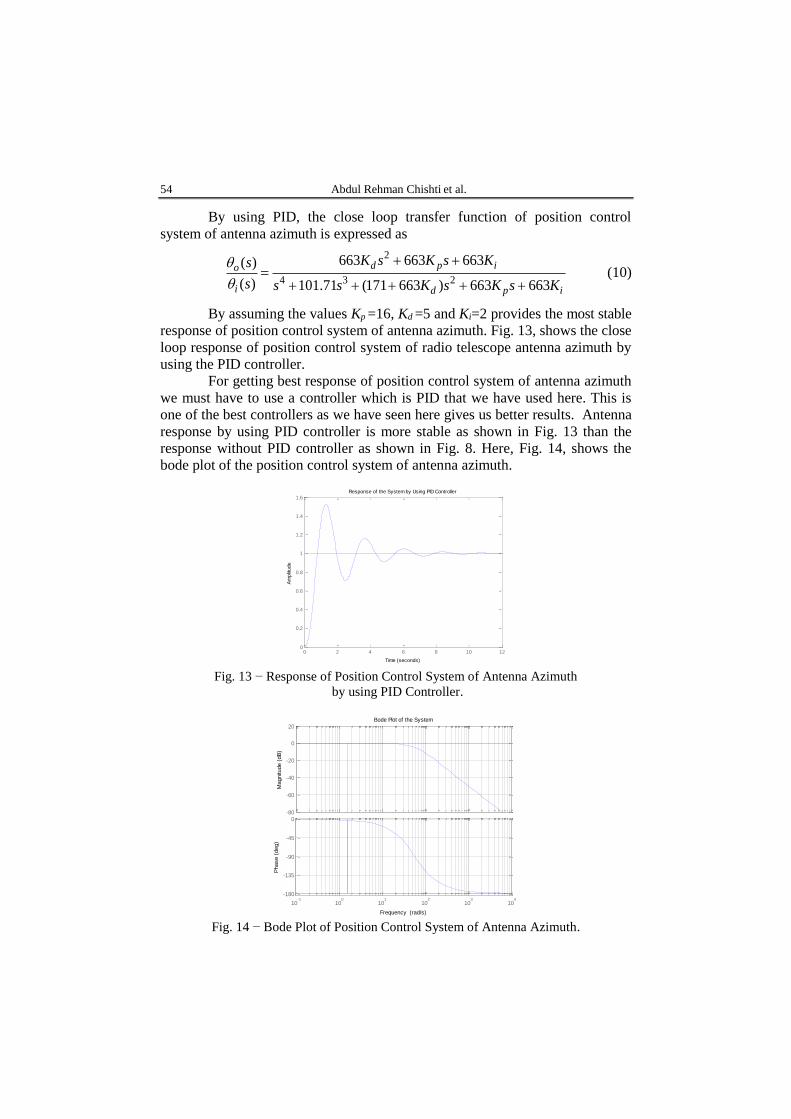
By using PID, the close loop transfer function of position control

system of antenna azimuth is expressed as

2

4 3 2

663 663 663( )

( ) 101.71 (171 663 ) 663 663

d p io

i d p i

K s K s Ks

s s s K s K s K

(10)

By assuming the values Kp =16, Kd =5 and Ki=2 provides the most stable

response of position control system of antenna azimuth. Fig. 13, shows the close

loop response of position control system of radio telescope antenna azimuth by

using the PID controller.

For getting best response of position control system of antenna azimuth

we must have to use a controller which is PID that we have used here. This is

one of the best controllers as we have seen here gives us better results. Antenna

response by using PID controller is more stable as shown in Fig. 13 than the

response without PID controller as shown in Fig. 8. Here, Fig. 14, shows the

bode plot of the position control system of antenna azimuth.

0 2 4 6 8 10 120

0.2

0.4

0.6

0.8

1

1.2

1.4

1.6

Response of the System by Using PID Controller

Time (seconds)

Am

plit

ude

Fig. 13 − Response of Position Control System of Antenna Azimuth

by using PID Controller.

-80

-60

-40

-20

0

20

Magnitu

de (

dB

)

10-1

100

101

102

103

104

-180

-135

-90

-45

0

Phase (

deg)

Bode Plot of the System

Frequency (rad/s) Fig. 14 − Bode Plot of Position Control System of Antenna Azimuth.


55

4. Response of the System by Using LQR Controller

Linear Quadratic Regulator (LQR) is one of the modern controllers

nowadays. It uses state space approach to analyse and controlling of such type

of systems. It is very simple to work with multi output system by using state

space method.

The results of the PID Controller are enhanced considering the

disturbance in the system, the use of LQR controller is necessary. In this section

we have designed the observer and after that implemented with the LQR controller.

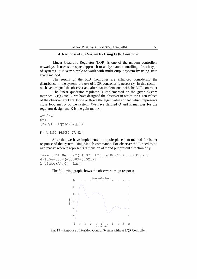
The linear quadratic regulator is implemented on the given system

matrices A,B,C and D. we have designed the observer in which the eigen values

of the observer are kept twice or thrice the eigen values of Ac, which represents

close loop matrix of the system. We have defined Q and R matrices for the

regulator design and K is the gain matrix.

Q=C’*C

R=1

[K,P,E]=lqr(A,B,Q,R)

K = [1.5190 16.6030 27.4624]

After that we have implemented the pole placement method for better

response of the system using Matlab commands. For observer the L need to be

nxp matrix where n represents dimension of x and p represent direction of y.

Lam= [1*1.0e+002*(-1.07) 4*1.0e+002*(-0.083-0.02i)

4*1.0e+002*(-0.083+0.02i)]

L=place(A',C', Lam)

The following graph shows the observer design response.

0 1 2 3 4 5 6 7 8 9 100

0.5

1

1.5

2

2.5

3

Time (seconds)

Am

plit

ude

Response of the System

Fig. 15 − Response of Position Control System without LQR Controller.


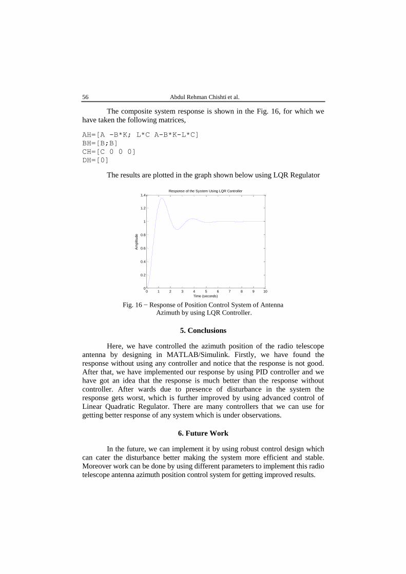
The composite system response is shown in the Fig. 16, for which we

have taken the following matrices,

AH=[A -B*K; L*C A-B*K-L*C]

BH=[B;B]

CH=[C 0 0 0]

DH=[0]

The results are plotted in the graph shown below using LQR Regulator

0 1 2 3 4 5 6 7 8 9 100

0.2

0.4

0.6

0.8

1

1.2

1.4

Time (seconds)

Am

plit

ude

Response of the System Using LQR Controller

Fig. 16 − Response of Position Control System of Antenna

Azimuth by using LQR Controller.

5. Conclusions

Here, we have controlled the azimuth position of the radio telescope

antenna by designing in MATLAB/Simulink. Firstly, we have found the

response without using any controller and notice that the response is not good.

After that, we have implemented our response by using PID controller and we

have got an idea that the response is much better than the response without

controller. After wards due to presence of disturbance in the system the

response gets worst, which is further improved by using advanced control of

Linear Quadratic Regulator. There are many controllers that we can use for

getting better response of any system which is under observations.

6. Future Work

In the future, we can implement it by using robust control design which

can cater the disturbance better making the system more efficient and stable.

Moreover work can be done by using different parameters to implement this radio

telescope antenna azimuth position control system for getting improved results.


57

Acknowledgments. We are grateful to every person who have helped us in

completing this project on time and in an effective way. We are equally thankful Engr.

Usman Ali khan and Engr. Jawad Masud. Regarding our project they support us and

provided us a lot of help in different matters. They also provide us moral support in

suggesting the outlines and correcting the doubts regarding our project. Last but not

least, we are thankful to everyone who have helped us.

REFERENCES

Evans W.R., Graphical Analysis of Control Systems. Transactions of the AIEE, 67,

547– 551, 1948.

Franklin G., Powell F., Emami-Naeini A., Feedback Control of Dynamic Systems. 4th

Ed., Addison-Wesley Publishing Company, 2002.

Kalman R.E., On the General Theory of Control Systems. IRE Transactions on

Automatic Control, 4, 3, 110, 1959. Abstract. Full Paper Published in

Proceedings of the 1st IFAC Congress, Moscow, 1960.

Kamen E.W., Industrial Control and Manufacturing. 1st Ed., Academic Press, 1999.

Minorsky N., Directional Stability of Automatically Steered Bodies. Journal of the

American Society of Naval Engineering, 34, 2, 280–309, 1922.

Nise N.S, Control System Engineering. 6th Ed., John Wiley & Sons, 2000.

Okumus H.I., Sahin E., Akyazi O., Antenna Azimuth Position Control with Classical

PID and Fuzzy Logic Controllers. IEEE Transaction on Education, 2012.

Xuan L., Estrada J., Digiacomandrea J., Antenna Azimuth Position Control System

Analysis and Controller Implementation. Term Project, 2009.

Ziegler J.G., Nichols N.B., Optimum Settings for Automatic Controllers. Transactions

of the ASME, 64, 759–768, 1942.

PROIECTAREA ŞI ANALIZA ÎN MEDIUL MATLAB/SIMULINK A UNUI

SISTEM DE CONTROL AL AZIMUTULUI UNUI RADIOTELESCOP

FOLOSIND REGULATOARE PID & LQR

(Rezumat)

Un sistem de control al poziţie converteşte o comandă generată de o poziţie de

intrare într-o poziţie de ieşire. Radiotelescoapele, unităţile de stocare dintr-un calculator

şi braţele robotizate conţin multe aplicaţii ale sistemului de control al poziţiei. În această

lucrare se evaluează o arhitectură proiectată pentru controlul azimutului unui

radiotelescop. Răspunsul sistemului este analizat, rezultatele fiind obţinute în urma

utilizării unui regulator PID. Aceste rezultatele sunt îmbunătăţite prin adăugarea unui

regulator LQ. Evaluarea performanţelor relevă rezultate mult mai bune pentru abordarea

bazată pe LQ decât rezultatele obţinute de abordarea PID.

Documents

radio telescope antenna azimuth position control system design and