Embed Size (px)
Citation preview
O
TTO
-VO
N-G
UE
R
ICKE-UNIVERSIT
ÄT
MA
GD
EB
UR
G
Otto–von–Guericke–Universität Magdeburg
Studienarbeit
Ranking and importance in
complex networksvon
Florian Knorn(* xxx Dez. 1981 in Berlin)
3. Oktober 2005
Eingereicht an die: Otto–von–Guericke–Universität MagdeburgFakultät für Elektrotechnik und InformationstechnikInstitut für AutomatisierungstechnikUniversitätsplatz 2Postfach 4120, 39016 MagdeburgDeutschland
Prüfer: Prof. Jörg Raisch
Betreuer: Dr. Oliver MasonProf. Robert Shorten
Hamilton InstituteNational University of IrelandMaynooth, Co. KildareIreland


Meiner Familie

Table of contents
Outline and objectives vii
Preface ix
Acknowledgments . . . . . . . . . . . . . . . . . . . . . . . . . . . . . . ix
Declaration of originality . . . . . . . . . . . . . . . . . . . . . . . . . . x
Introduction xi
1 Notions from Graph theory 1
1.1 Introduction . . . . . . . . . . . . . . . . . . . . . . . . . . . . . . 1
1.2 Basic definitions . . . . . . . . . . . . . . . . . . . . . . . . . . . . 1
1.3 Matrices associated with graphs . . . . . . . . . . . . . . . . . . . 4
1.4 Characteristic values . . . . . . . . . . . . . . . . . . . . . . . . . . 9
2 Random graphs 17
2.1 Introduction . . . . . . . . . . . . . . . . . . . . . . . . . . . . . . 17
2.2 The Erdös–Rényi Model . . . . . . . . . . . . . . . . . . . . . . . . 18
2.3 The Watts–Strogatz or “small–world” Model . . . . . . . . . . . . . 23
2.4 The Barabási–Albert or “scale–free” Model . . . . . . . . . . . . . . 28
2.5 Comparison and applications . . . . . . . . . . . . . . . . . . . . . 33
3 Ranking schemes 37
3.1 Introduction . . . . . . . . . . . . . . . . . . . . . . . . . . . . . . 37
3.2 Node degrees . . . . . . . . . . . . . . . . . . . . . . . . . . . . . 38
3.3 HITS . . . . . . . . . . . . . . . . . . . . . . . . . . . . . . . . . . 38
3.4 PageRank . . . . . . . . . . . . . . . . . . . . . . . . . . . . . . . 44
3.5 Centrality measures . . . . . . . . . . . . . . . . . . . . . . . . . . 50
3.6 Damage . . . . . . . . . . . . . . . . . . . . . . . . . . . . . . . . 53
4 Robustness 57
4.1 Introduction . . . . . . . . . . . . . . . . . . . . . . . . . . . . . . 57
4.2 Perturbations . . . . . . . . . . . . . . . . . . . . . . . . . . . . . 57
4.3 Measures of deviation . . . . . . . . . . . . . . . . . . . . . . . . . 59
4.4 Quantitative assessment . . . . . . . . . . . . . . . . . . . . . . . . 63
4.5 Theoretical results . . . . . . . . . . . . . . . . . . . . . . . . . . . 75
v
vi TABLE OF CONTENTS
5 Application to real data 795.1 Introduction . . . . . . . . . . . . . . . . . . . . . . . . . . . . . . 79
5.2 Examination of the data . . . . . . . . . . . . . . . . . . . . . . . . 80
5.3 Identifying essentiality . . . . . . . . . . . . . . . . . . . . . . . . . 86
5.4 Robustness of the identification of essentiality . . . . . . . . . . . . 89
Conclusion 93
A Additional theorems 95A.1 Connectedness and irreducibility . . . . . . . . . . . . . . . . . . . 95
A.2 Perron–Frobenius Theorem . . . . . . . . . . . . . . . . . . . . . . 96
B Additional plots 97B.1 Sensitivity . . . . . . . . . . . . . . . . . . . . . . . . . . . . . . . 97
List of Symbols 107
Bibliography 109
Outline and objectives
In the recent past, there has been enormous interest across a number of researchcommunities in the analysis of complex networks. One of the major motivationsfor this is the importance of such networks in a variety of diverse application areas,including power systems, the Internet and World Wide Web (WWW), social networks,transportation networks, food webs and biological networks. Furthermore, it wasrecently established in a sequence of papers that the random graph models, introducedby Erdös and Rényi, traditionally used to model complex networks do not accuratelycapture many of the key properties of networks that occur in the real world. This ledto the introduction of several new network models including the small–world modelof Watts and Strogatz (WS) and the scale–free models of Barabási and Albert (BA).A key issue in the analysis of complex networks in several fields is how to identifycritical or important nodes within a network. One familiar example of this is providedby the various algorithms developed to rank pages on the WWW in terms of theirimportance or relevance to a specific search query; the most famous such algorithmbeing the PageRank algorithm which underpins the Google search engine. A novelinteresting application of similar ideas has arisen in the analysis of biological networkssuch as protein–protein interaction and transcriptional networks, where algorithmsfor the identification of critical genes or proteins have potential applications in drugdesign.
This project has a number of objectives. Firstly, the student should become fa-
miliar with the basics of Graph Theory and the main statistics used to characterize
graph structure as well as the major algorithms used to rank pages on the WWW;
namely the HITS algorithm of Kleinberg and the PageRank algorithm of Brin and
Page. Specifically, the student should be able to implement these algorithms in Mat-
lab or an appropriate programming language, and explain clearly the theory behind
the algorithms and their convergence properties. The student should also be able
to describe a number of other measures of importance in networks including dam-
age, status and excentricity. Secondly, the student should survey the recent models
of complex networks, be able to describe and quantify the main properties of these
models, and should produce programs to generate and analyze the major network
models introduced in recent years. The third strand of the project relates to the
application of ranking algorithms to networks subject to uncertainty. This is of par-
ticular relevance in biological applications where network data is always considerably
noisy. The student should quantitatively assess the sensitivity of PageRank and HITS
to various types of uncertainty in network structure, and compare the sensitivity of
these measures to that of other traditional notions of network importance such as
status.
vii

Preface
Think where man’s glory most begins and ends,
And say my gloray was I had such friends.
The Municipal Gallery Re–Visited
William B. Yeats
Acknowledgments
There are many people who contributed to the effort that is my Studienarbeit.Without their generous assistance it would not have been possible to write it.
Firstly I would like to express my deep gratitude to Prof. Jörg Raisch. Heestablished the connection to the Hamilton Institute and arranged my stay here.In all the years at university I have seen him as my mentor and I would liketo thank him for his great teaching, advice and continuing support throughoutthe years.
Secondly I would like to thank in part the Studienstiftung des deutschenVolkes (“German National Academic Foundation”) and the Hamilton Institute(ultimately the Science Foundation Ireland, grant number 04/In1/I478) fortheir generous financial support. Without that, it would have been very hardfor me to afford the six months I spent here in Maynooth.
Next, I’d like to thank Prof. Robert Shorten from the Hamilton Institute fortaking a chance on an unknown young man from Germany and being mostlyconvinced that I could do this. His wise advice and experience he sharedextending way beyond aspects related to this Studienarbeit were a great honourto receive and follow, not to forget the cracking basketball games at the end ofthe weeks.
The person, however, I worked most closely with and who invested a lot oftime and thoughts in me is Dr. Oliver Mason. It will be hard to leave him, hissagacious advice as well as his humor behind, and I thank him deeply for allhis help, support, ideas and patience.
I also feel deeply honoured and grateful for the opportunity to work atthe Hamilton Institute. It is such a high–profile yet friendly and open mindedenvironment that I will miss a lot. It was a pleasure to sit in the countlessseminars held by many impressive international scientists. Furthermore I ammost thankful for the many opportunities for my future that have arisen frommy stay in the institute.
Moreover, I would like to thank the following people, colleagues, office matesor Erasmus students for their help and for being many welcome sources of dis-
ix
x PREFACE
traction, adding some “live” to the “work” and having those many cool parties.In alphabetical order with titles omitted: Amandine Mukeka, Anat Zil–Bar,Anthony Ng, Barak Pearlmutter, Baruch Even, Berenice Sanchez, Camille Hy-ron, Carlos Villegas, Caroline Terrisse, Cornelia Nell, David Malone, DelphineWibaux, Fabian Wirth, Ian Dangerfield, Ian Robertson, Kai Wulff, Kate Mo-riarty, Laura Karsties, Lea Steppacher, Livia Ruiz, Luke O’Shaughnessy, MarkVerwoerd, Marta Barreras, Mary Quirke, Mehmet Akar, Peter Wellstead, RadeStanojevich, Richard Middleton, Rosemary Hunt, Santiago Jaramillo, SelimSolmaz, Steven Strachan, Tianji Li, Ulf Schaper, Zhangping Du, . . . and many,many more.
I would also like to thank my favorite pub in Maynooth, the Roost, forthe nice atmosphere for having all those Pints o’ Guinness, Jameson or Bush-mills Whiskeys, the little dancing area upstairs and the pub grub served. Andthanks to Amandine’s great Salsa classes twice a week we always had a greattime those Sunday nights at the SamSara in Dublin.
Finally, I could never overstate my gratitude toward my family and closefriends for their continuous help and moral support, especially during the darkermoments at the beginning of my stay here.
∗ ∗ ∗
Declaration of originality
I hereby declare that this thesis and the work reported herein was composedand originated entirely by myself. Information derived from the published andunpublished work of others is acknowledged in the text and a list of referencesis given in the bibliography.
Magdeburg, 7. Oktober 2005
Florian Knorn
Introduction
Graphs are a very versatile and powerful means of modelling complex, “net-worklike” systems. This rather abstract mathematical construct can be used tocapture interactions between a large number of components or agents, and, be-yond allowing for an intuitive graphical representation, provides us with manymethods to analyse and manipulate the system we are interested in.
We will use the first chapter to present and review basic notions from graphtheory to have a clear framework to build our further investigations on.
Graph theory is an established discipline in discrete mathematics, but un-til fairly recently only relatively small graphs have been considered. However,advances in many fields have brought along tremendously more complex andlarger graphs. For instance, the concept of a graph has been used to describenetworks as large and diverse as the internet, neural networks of living crea-tures, telephone networks or social relations.
As in most other disciplines people tried to create models that reflect orimitate the properties of real world systems. The most prominent and seminalof these is certainly the classical random graph model by Erdös and Rényi.
But this rather artificial model cannot capture many of the remarkableaspects of real world networks. The urging need for better models has beensatisfied to some extent by the introduction of more complicated models in therecent past, like the small–world model by Watts and Strogatz, or the scale–freemodel by Barabási and Albert. The second chapter of this document focuseson these three graph models. We shall shed some light on their characteristicsas well as on how they compare with each other, and with real world networks.
The increasing complexity and amount of data becoming available fromreal world applications but also randomly generated networks brought alongpressing needs for methods and algorithms to analyse them. This can involvedetermining global properties of the network, i. e. characterising the network asa whole, but also local or individual measures for groups of nodes or individualnodes.
A very common task would be to identify important or critical nodes of anetwork. An important application is the retrieval of relevant information froma knowledge base in the form of a large network, a very prominent examplebeing the world wide web. Finding the right piece of information then boilsdown to finding important or relevant nodes relative to the query. The knowl-edge of key nodes could also be used to either target them, as one would wantto do for example in networks describing the spread of epidemics — or protectthem, like in networks representing some sort of infrastructures for instance.
It is the aim of the third chapter to review some of the highly ingeniousranking schemes that try to answer the need for identifying important nodes
xi
xii INTRODUCTION
in a network. These include the famous PageRank algorithm, the fairly recentmeasure called “damage”, but also a number of classical topological measuresthat have been established in relation with resource allocation problems.
Networks drawn from real world systems are usually based on some sort ofphysical measurement which in cases may introduce considerable amounts ofnoise. Before using a ranking scheme it is crucial to evaluate its sensitivity towrong, incomplete, missing or uncertain data.
This is especially important in domains like biology, where one has to facesignificant amounts of noise in the data due to numerous reasons. A schemethat inverts the order of the nodes in the ranking when only a few edges arechanged would clearly be of little practical use.
For that reason, we shall evaluate in the fourth chapter the robustness ofthe introduced ranking schemes with respect to perturbations in the network.We establish empirical ways of measuring deviations between rankings and usethese to analyse the sensitivity of the ranking schemes on randomly generatedscale–free graphs.
Another question that needs to be addressed is the actual usefulness of therankings, i. e. the ability of the ranking schemes to actually identify essentialnodes with respect to certain criteria (based on the application). Obviously,this has to be done in conjunction with real data where we know which nodesare important and which are not.
We evaluate this on biological data in Chapter 5 using three differentprotein–protein interaction networks that have been established recently. Thesedatasets provide us with the networks as well as the set of nodes that are knowto be essential to the survival of the organism. In particular, we investigatethe connection between the essentiality of nodes and the amount of importanceattributed to them by the different ranking schemes.
All the algorithms used in the preparation of this document have beenwritten in Matlab and are available on the accompanying web page of thisdocument, [36]. Most of them are commented on and explained in the text,together with the core of their code. We used the freely available programPajek, [7], to generate the graphics. The three datasets from Chapter 5 canalso be found in [65].
C H A P T E R 1
Notions from Graph theory
A few basic notions from graph theory will be
recalled, introducing various definitions and
terminology, four types of matrices associated with
graphs and some characteristic values.
1.1 Introduction
The notion of a “graph” as currently used in graph theory was first introducedin the first half of the eighteenth century by the swiss mathematician LeonhardEuler, who tried to solve the Königsberg bridge problem1. It is said that about100 years later the english mathematician James J. Sylvester coined the word“graph” as we currently know it.
A surprisingly large number of systems have a complex, weblike structurewhich can be described using graphs. So clearly, results from graph theoryallow investigation — and explanation — of many properties of these systems.
Examples can be drawn from many aspects of life, [2]. Just to name afew, large graphs have been used to describe the hyperlink structure of theworld wide web, the system of routers and computers forming the internet,complex chemical reaction networks in a cell, steps in protein foldings, neuralnetworks, power grids, cellular and phone networks, collaboration networks ofscientists or actors, word occurrences or patterns in linguistics, power grids,transportation or traffic networks.
This chapter discusses several basic notions from graph theory to facilitateour later discussion of random graphs.
1.2 Basic definitions
1.2.1 Graphs
Let’s start off with a very general definition of a graph:
Definition 1.1 (Graph)A graph G is a couple of finite sets (V, E), where V is the set of nodes,
and E is the set of edges between the nodes, E ⊆{
(u, v)∣
∣u, v ∈ V}
.
1 At the time, the city of Königsberg consisted of two islands in a river, linked by sevenbridges. On his morning walks, Euler wondered if there was a route beginning and endingat the same point and traversing all the brigdes exactly once. To find out whether this waspossible or not, Euler modeled the problem with a graph . . .
1
2 CHAPTER 1. NOTIONS FROM GRAPH THEORY
Usually, one distinguishes between two major types of graphs: directed
graphs (also called digraphs) and undirected graphs.A graph is said to be undirected if the adjacency relation defined by the
edges is symmetric (i. e. E ⊆{
{u, v}∣
∣u, v ∈ V}
is made up of sets of nodesrather than ordered pairs). Otherwise the graph is called directed.
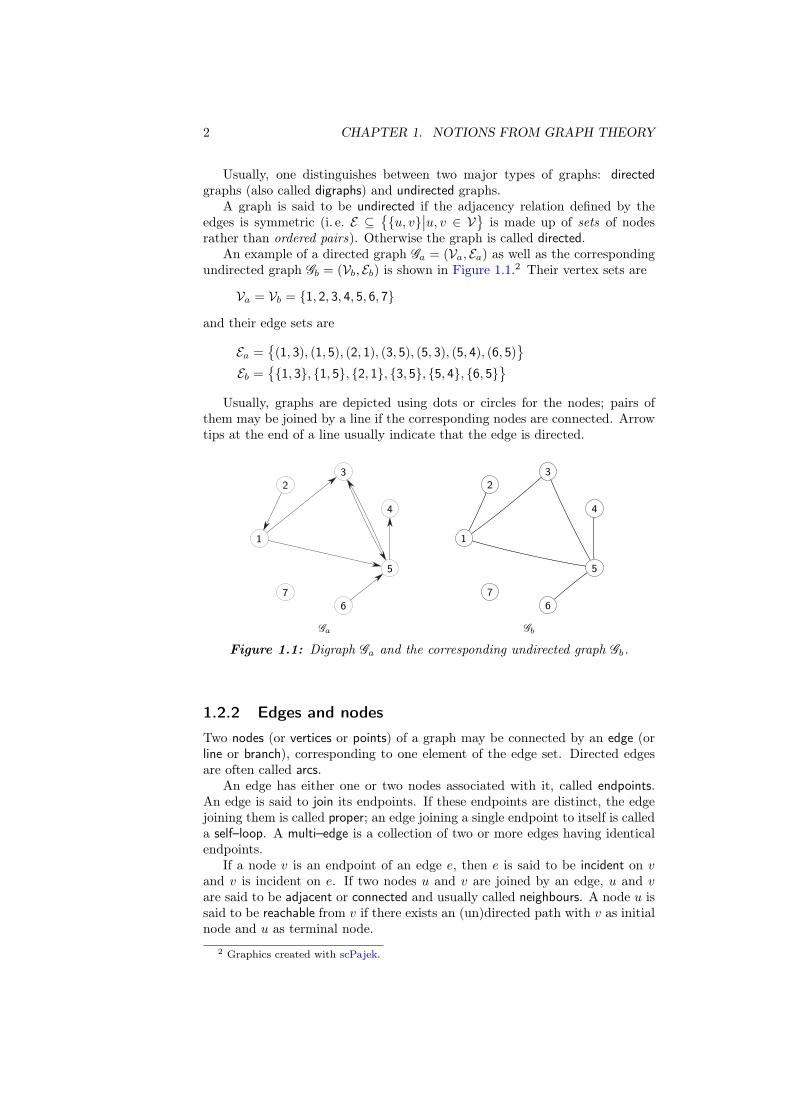
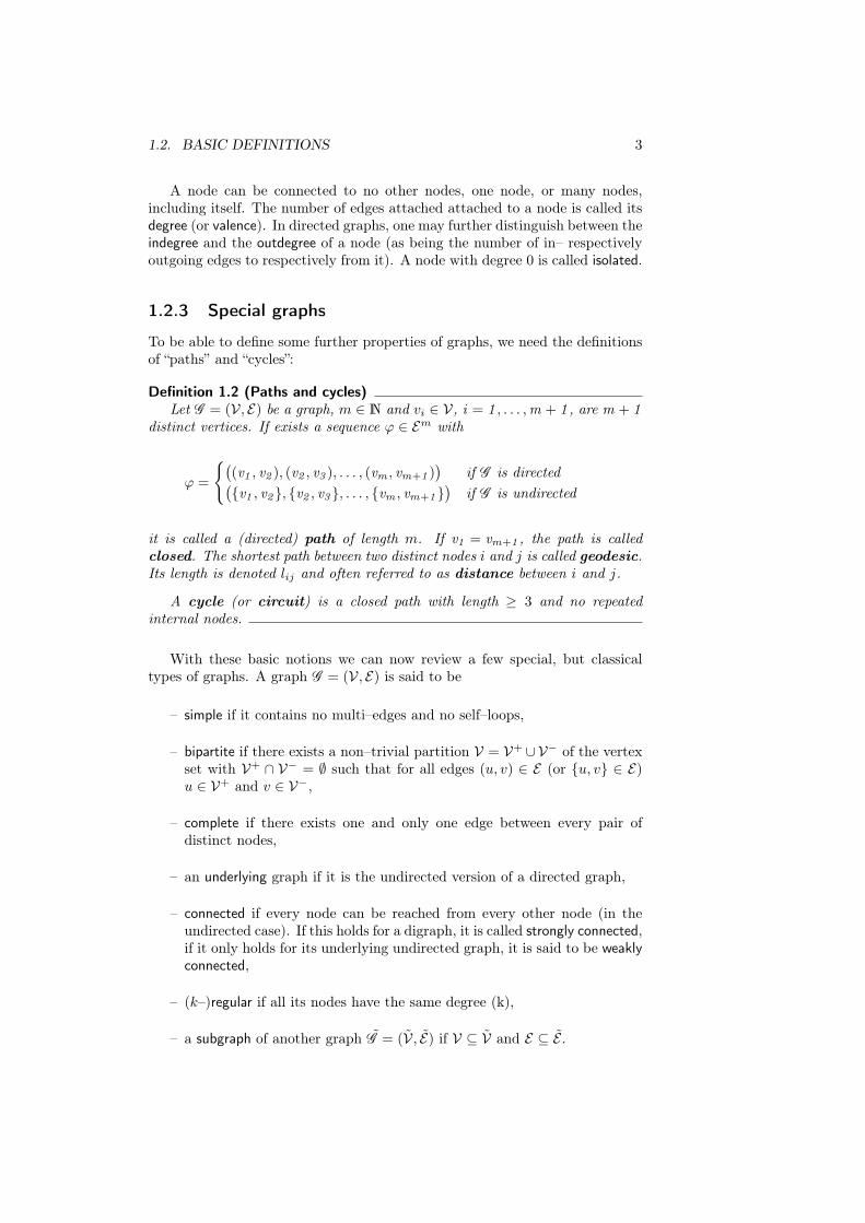
An example of a directed graph Ga = (Va, Ea) as well as the correspondingundirected graph Gb = (Vb, Eb) is shown in Figure 1.1.2 Their vertex sets are
Va = Vb = {1, 2, 3, 4, 5, 6, 7}
and their edge sets are
Ea ={
(1, 3), (1, 5), (2, 1), (3, 5), (5, 3), (5, 4), (6, 5)}
Eb ={
{1, 3}, {1, 5}, {2, 1}, {3, 5}, {5, 4}, {6, 5}}
Usually, graphs are depicted using dots or circles for the nodes; pairs ofthem may be joined by a line if the corresponding nodes are connected. Arrowtips at the end of a line usually indicate that the edge is directed.
1
23
4
5
6
7
Ga
1
23
4
5
6
7
Gb
Figure 1.1: Digraph Ga and the corresponding undirected graph Gb.
1.2.2 Edges and nodes
Two nodes (or vertices or points) of a graph may be connected by an edge (orline or branch), corresponding to one element of the edge set. Directed edgesare often called arcs.
An edge has either one or two nodes associated with it, called endpoints.An edge is said to join its endpoints. If these endpoints are distinct, the edgejoining them is called proper; an edge joining a single endpoint to itself is calleda self–loop. A multi–edge is a collection of two or more edges having identicalendpoints.
If a node v is an endpoint of an edge e, then e is said to be incident on vand v is incident on e. If two nodes u and v are joined by an edge, u and vare said to be adjacent or connected and usually called neighbours. A node u issaid to be reachable from v if there exists an (un)directed path with v as initialnode and u as terminal node.
2 Graphics created with scPajek.
1.2. BASIC DEFINITIONS 3
A node can be connected to no other nodes, one node, or many nodes,including itself. The number of edges attached attached to a node is called itsdegree (or valence). In directed graphs, one may further distinguish between theindegree and the outdegree of a node (as being the number of in– respectivelyoutgoing edges to respectively from it). A node with degree 0 is called isolated.
1.2.3 Special graphs
To be able to define some further properties of graphs, we need the definitionsof “paths” and “cycles”:
Definition 1.2 (Paths and cycles)Let G = (V, E) be a graph, m ∈ N and vi ∈ V, i = 1 , . . . ,m + 1 , are m + 1
distinct vertices. If exists a sequence ϕ ∈ Em with
ϕ =
{
(
(v1 , v2 ), (v2 , v3 ), . . . , (vm , vm+1 ))
if G is directed(
{v1 , v2}, {v2 , v3}, . . . , {vm , vm+1})
if G is undirected
it is called a (directed) path of length m. If v1 = vm+1 , the path is calledclosed. The shortest path between two distinct nodes i and j is called geodesic.Its length is denoted lij and often referred to as distance between i and j.
A cycle (or circuit) is a closed path with length ≥ 3 and no repeatedinternal nodes.
With these basic notions we can now review a few special, but classicaltypes of graphs. A graph G = (V, E) is said to be
– simple if it contains no multi–edges and no self–loops,
– bipartite if there exists a non–trivial partition V = V+ ∪V− of the vertexset with V+ ∩ V− = ∅ such that for all edges (u, v) ∈ E (or {u, v} ∈ E)u ∈ V+ and v ∈ V−,
– complete if there exists one and only one edge between every pair ofdistinct nodes,
– an underlying graph if it is the undirected version of a directed graph,
– connected if every node can be reached from every other node (in theundirected case). If this holds for a digraph, it is called strongly connected,if it only holds for its underlying undirected graph, it is said to be weakly
connected,
– (k–)regular if all its nodes have the same degree (k),
– a subgraph of another graph G = (V, E) if V ⊆ V and E ⊆ E .
4 CHAPTER 1. NOTIONS FROM GRAPH THEORY
Note: In the following we will only focus on simple graphsas most of the graphs we will be encountering in this paperare simple graphs!
Furthermore we will always suppose that a graph G = (V, E)we are investigating has n = |V| nodes and that they arenumbered and explicitly ordered 1, . . . , n.
1.3 Matrices associated with graphs
In order to work with graphs, the representation using two sets is not veryuseful. In fact, all the information contained within these two set (with theexception of the names of the nodes, if they are not explicitly numbered 1 ton) can be contained in a matrix.
1.3.1 Adjacency matrix
One of the most common — and probably the most intuitive matrix associatedwith graphs is the following.
Definition 1.3 (Adjacency matrix)The n× n adjacency matrix A of a graph G = (V, E) is defined as
aij =
{
1 if (vi, vj) ∈ E resp. {vi, vj} ∈ E0 otherwise
(1.1)
and hence is symmetric if G is an undirected graph.
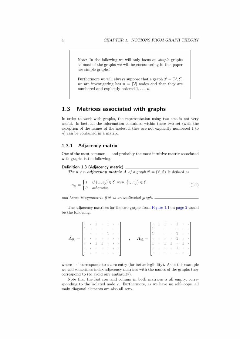
The adjacency matrices for the two graphs from Figure 1.1 on page 2 wouldbe the following:
AGa=
· · 1 · 1 · ·1 · · · · · ·· · · · 1 · ·· · · · · · ·· · 1 1 · · ·· · · · 1 · ·· · · · · · ·
, AGb=
· 1 1 · 1 · ·1 · · · · · ·1 · · · 1 · ·· · · · 1 · ·1 · 1 1 · 1 ·· · · · 1 · ·· · · · · · ·
where “ · ” corresponds to a zero entry (for better legibility). As in this examplewe will sometimes index adjacency matrices with the names of the graphs theycorrespond to (to avoid any ambiguity).
Note that the last row and column in both matrices is all empty, corre-sponding to the isolated node 7. Furthermore, as we have no self–loops, allmain diagonal elements are also all zero.
1.3. MATRICES ASSOCIATED WITH GRAPHS 5
Connected graphs
In the example above, as node 7 cannot be reached from any other node, Gb isnot connected. The property of a graph being either connected or not is closelyrelated to a certain property of its adjacency matrix.
It’s a well know fact, and stated formally in Theorem A.1 on page 95 inthe Appendix, that a graph is (strongly) connected if and only if its adjacencymatrix is irreducible in the sense of the following definition.
Definition 1.4 (Irreducibility of a matrix)A matrix A ∈ R
n×n with is said to be reducible if either
(i) n = 1 and A = 0 ; or
(ii) n ≥ 2 , there is a permutation matrix Π n ∈ Rn×n and there is some
integer r with 1 ≤ r ≤ n − 1 such that
ΠTnAΠ n =
[
B C
0 D
]
(1.2)
where B ∈ Rr×r, D ∈ R
(n−r)×(n−r), C ∈ Rr×(n−r) and 0 ∈ R
(n−r)×r isthe zero matrix.
Note that this definition does not require the blocks B, C, and D to havenonzero entries, but only that one should be able to get an (n− r)–by–r blockof 0 entries in the indicated position by some sequence of row and columninterchanges.
Powers of the adjacency matrix
Looking at the adjacency matrix A of a graph with n nodes, we basically seethe locations of paths of length 1 between each pair of nodes (aij = 1 perdefinition means there is an edge between node i and j). Strictly speaking, wesee the number of paths of length 1 between each pair of nodes, as we will seenow.
It is a fact that if we look at a positive power of the adjacency matrix, Am,m ∈ N, each entry am
ij tells us the number of paths of length m between nodei and node j.3. This can easily be seen if we recall that
a2ij =
n∑
k=1
aikakj
Here, the value of a2ij corresponds to the number of cases where there are two
edges (i, k) and (k, j), i. e. the number of different paths of length two that gofrom node i to node j. This can then be easily extended to higher powers of A.
With this in mind, it is quite immediate to see that a matrix A is irreducibleif and only if some positive power of (A + id) is strictly positive (the additionof the identity matrix is needed to ensure the fact that every node is reachablefrom itself).
3 amij denotes element (i, j) of Am, see also the List of Symbols on page 108.
6 CHAPTER 1. NOTIONS FROM GRAPH THEORY
1.3.2 Laplacian matrix
Another commonly used matrix for analyzing graphs is the Laplacian matrix,which we now define.
Definition 1.5 (Laplacian matrix)For an undirected graph G = (V, E) with n = |V| nodes, its n × n Lapla-
cian matrix (also called graph Laplacian, just Laplacian, Admittance–or Kirchhoff matrix) LG is defined as the difference between its degree matrixand its adjacency matrix:
LG = DG −AG
where DG = diag(k1, k2, . . . , kn), ki being the degree of node i.
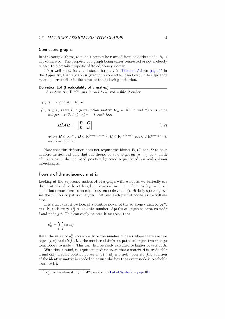
To illustrate this definition, the Laplacian of Gb from Figure 1.1 on page 2would be
LGb=
3 −1 −1 · −1 · ·−1 1 · · · · ·−1 · 3 · −1 · ·· · · 1 −1 · ·−1 · −1 −1 4 −1 ·· · · · −1 1 ·· · · · · · ·
The definition of the Laplacian allows for it to have a couple of importantand elementary properties:
Proposition 1.1 (Positive semidefiniteness of the Laplacian)For an undirected graph G = (V, E) the following hold for its Laplacian:
(i) LG is positive semidefinite.
(ii) The smallest eigenvalue of LG is λ1 = 0 and a corresponding eigenvectoris 1n, the n–element column vector with all ones.
(iii) Let λ1 ≤ λ2 ≤ . . . ≤ λn be the eigenvalues of LG . If G is connected, thenλ2 > 0 .
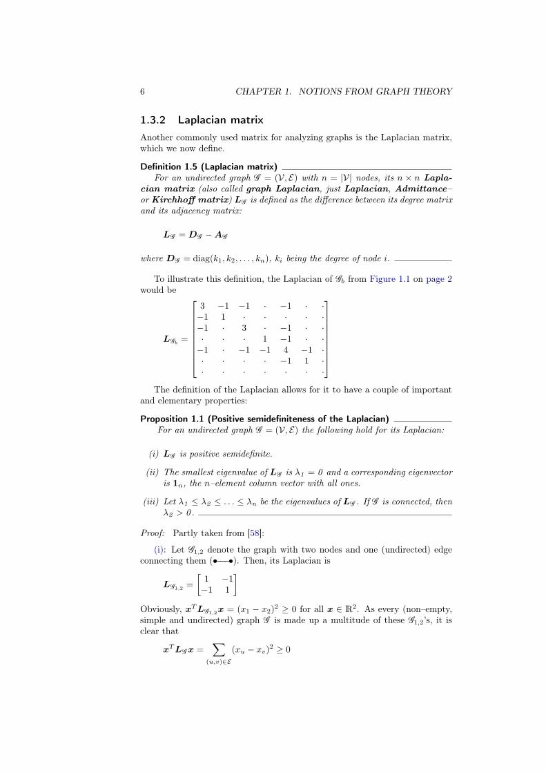
Proof: Partly taken from [58]:
(i): Let G1,2 denote the graph with two nodes and one (undirected) edgeconnecting them (•−−−•). Then, its Laplacian is
LG1,2=
[
1 −1−1 1
]
Obviously, xT LG1,2x = (x1 − x2)
2 ≥ 0 for all x ∈ R2. As every (non–empty,
simple and undirected) graph G is made up a multitude of these G1,2’s, it isclear that
xT LG x =∑
(u,v)∈E
(xu − xv)2 ≥ 0
1.3. MATRICES ASSOCIATED WITH GRAPHS 7
for all x ∈ Rn.
(ii): As the sum over a row from AG is equal to the degree of the corre-sponding node, the sum over a row of LG is always zero. Hence LG 1n = 0n.
(iii): Let ν be an eigenvector of LG of eigenvalue 0. Then LG ν = 0n and
νT LG ν =∑
(u,v)∈E
(νu − νv)2 = 0
Thus for each pair of nodes (u, v) connected by an edge, we must have νu = νv.As the graph is connected, we have νu = νv for all pairs of nodes (u,v), whichimplies that ν is a scalar multiple of 1n. Thus, the eigenspace associated withλ1 = 0 has dimension 1, and since LG is positive semidefinite, λ2 must bestrictly positive. �
As a result from linear algebra, the fact that LG is always positive semidef-inite implies that all its eigenvalues are real and nonnegative, which was usedin the proof of (iii).
This property has actually led Fiedler to consider the magnitude of λ2
as a measure of the connectedness of a graph [21], calling λ2 the algebraic
connectivity. Loosely speaking: the greater λ2, the more “connected” the graph.As the spectrum of a graph is made of the union of the spectra of its
connected components, the multiplicity of 0 as an eigenvalue of LG is equal tothe number of connected components4.
A number of different results using λ2 can found in [47], like bounds for thediameter, average path length or other characteristic values of a graph, [46].These are useful for extremely large networks that are out of scope of algorithmslike those shown in the next section.
Before moving on, let’s have a quick look at our example from Figure 1.1on page 2 again. There, the three smallest eigenvalues of LGb
are 0, 0, and ≃0.6314, indicating, that it has two connected components (that is the connectednodes 1 to 6 on the one hand, as well as the isolated node 7 on the other).
1.3.3 Distance matrix
Another matrix we are going to look at is the distance matrix. It contains allthe distance information of the graph, that is the shortest path lengths betweenany two (distinct) nodes.
We present here a somewhat customized definition of the distance matrix,allowing us to extend its classical definition to disconnected graphs.
Definition 1.6 (Distance matrix)For a given graph G = (V, E), its n× n distance matrix ∆. is given by
δij =
0 if i = j
lij if node i can be reached from node j
n if node i cannot be reached from node j
4 A connected component of a graph G1 is a connected subgraph G2 such that no subgraphof G1 that properly contains G2 is connected. In other words, a connected component is amaximal connected subgraph.

8 CHAPTER 1. NOTIONS FROM GRAPH THEORY
where n = |V| is the total number of nodes in the graph.
The usual definition of the distance matrix either demands connectedness,or, if not, sets the corresponding entries for disconnected nodes to infinity. Forour applications later we choose not to set it to infinity, as this does not allowfor any quantification to which extent a node is disconnected. This will beparticularly important when we look at centrality measures like excentricity,status and centroid value (see Section 3.5 on page 50).
Obviously, this matrix will be symmetric in the case of undirected graphs.One way of calculating it is mentioned in Footnote 7 on page 11.
In our example from Figure 1.1 on page 2, the distance matrix of the di-rected graph Ga is:
∆Ga=
· 7 1 2 1 7 71 · 2 3 2 7 77 7 · 2 1 7 77 7 7 · 7 7 77 7 1 1 · 7 77 7 2 2 1 · 77 7 7 7 7 7 ·
1.3.4 Incidence matrix
For reasons of completeness, let’s define a third type of matrix usually associ-ated with an undirected graph [47]:
Definition 1.7 (Incidence matrix)For a given directed graph G = (V, E), the |V| × |E| incidence matrix I
is defined by
ive =
−1 if edge e is directed to node v
1 if edge e is directed from node v
0 otherwise
In case of an undirected graph, first orient its edges arbitrarily, i. e. for eache ∈ E, choose one of its endpoints as the initial node, and the other as terminalnode.
Defining the incidence matrix for an undirected graph as above we have
LG = IG ITG (1.3)
independent of the orientation chosen for the edges [9]. This property canbe used for an alternative proof of Proposition 1.1(i) on page 6. Using theincidence matrix and the scalar product, we can write with Equation (1.3)
xT LG x = 〈LG x,x〉 = 〈IG ITG x,x〉 = 〈IT
G x, ITG x〉 ≥ 0
showing that the Laplacian of a graph is always positive semidefinite.

1.4. CHARACTERISTIC VALUES 9
For our small graph Ga from Figure 1.1 on page 2, the incidence matrixwould be:
IGa=
−1 1 1 · · · ·1 · · · · · ·· −1 · 1 −1 · ·· · · · · −1 ·· · −1 −1 1 1 1· · · · · · −1· · · · · · ·
Now that we gathered the necessary terminology we should take a look at somecharacteristic values associated with graphs.
1.4 Characteristic values
To be able to better classify and compare the topologies of the random networksencountered in the next chapter we need a number of local and global measuresassociated with networks.
As we could not find any practical implementations of algorithms that cal-culate or determine those measures — nor good hints on how to realise them —we had to come up with an exact way of calculating them as well as sufficientlyfast implementations for our purposes. For both reasons, we present with eachvalue the core routines of the Matlab programs that accompany this paper.5
1.4.1 Average node degree
As the name suggests, the definition is straightforward:
Definition 1.8 (Average node degree)The average node degree of an undirected graph G = (V, E) is defined as
〈k〉 =1
n
n∑
i=1
ki
where ki is the degree of node i and n = |V| ≥ 1 is the total number of nodes.
If G is a directed graph, then
〈k〉 =1
n
n∑
i=1
(
kini + kouti
)
where kini and kouti are the in– and outdegrees of node i.
The Matlab code for this value is also straightforward. One can easily seethat 〈k〉 = 2e/n, where e = |E| is the total number of edges. So in the m–file,
5 Implementations in lower level programming languages may differ significantly from theapproaches taken here, where we tried to avoid loops as much as possible and rather usedmatrix operations and built in routines of Matlab.
10 CHAPTER 1. NOTIONS FROM GRAPH THEORY
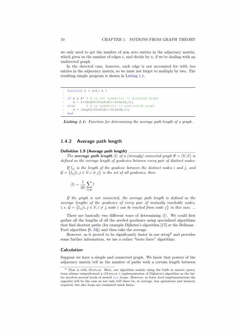
we only need to get the number of non–zero entries in the adjacency matrix,which gives us the number of edges e, and divide by n, if we’re dealing with anundirected graph.
In the directed case, however, each edge is not accounted for with twoentries in the adjacency matrix, so we must not forget to multiply by two. Theresulting simple program is shown in Listing 1.1.
1 function k = avk( A )
2
3 if A 6= A' % A is not symmetric => directed graph
4 k = 2*length(find(A))/size(A,1);
5 else % A is symmetric => undirected graph
6 k = length(find(A))/size(A,1);
7 end
Listing 1.1: Function for determining the average path length of a graph.
1.4.2 Average path length
Definition 1.9 (Average path length)The average path length 〈l〉 of a (strongly) connected graph G = (V, E) is
defined as the average length of geodesics between every pair of distinct nodes:
If lij is the length of the geodesic between the distinct nodes i and j, andG =
{
lij∣
∣i, j ∈ V, i 6= j}
is the set of all geodesics, then
〈l〉 =1
|G|∑
l∈G
l
If the graph is not connected, the average path length is defined as theaverage lengths of the geodesics of every pair of mutually reachable nodes,i. e. G =
{
lij∣
∣i, j ∈ V, i 6= j,node i can be reached from node j}
in this case.
There are basically two different ways of determining 〈l〉. We could firstgather all the lengths of all the needed geodesics using specialized algorithmsthat find shortest paths (for example Dijkstra’s algorithm [17] or the Bellman–Ford algorithm [8, 34]) and then take the average.
However, as it proved to be significantly faster in our setup6 and providessome further information, we use a rather “brute force” algorithm:
Calculation
Suppose we have a simple and connected graph. We know that powers of theadjacency matrix tell us the number of paths with a certain length between
6 That is with Matlab. Here, our algorithm mainly using the built–in matrix opera-tions always outperformed a (Matlab–) implementation of Dijkstra’s algorithm as the lat-ter involves several levels of nested for–loops. However, in lower level implementations theopposite will be the case as not only will there be, in average, less operations and memoryrequired, but also loops are evaluated much faster.
1.4. CHARACTERISTIC VALUES 11
each pair of nodes. Hence in order to determine the shortest path between twonodes i and j we can look at powers of the adjacency matrix and wait for theemergence of a non–zero value in the ij–th entry. So if for a certain m ∈ N
we have amij 6= 0 where for lower powers that entry was always zero, we can
conclude that the shortest path from node i to node j has length m.Effectively, all that needs to be done is keep track of the number of new
non–zero entries at each step (new power of A) and then calculate the average.To do so, we iteratively sum up the powers of A:
AΣ(m) = A0 + A1 + A2 + . . . + Am (1.4)
As the graph consists of n nodes, the shortest path between two nodes canhave at most length n − 1 (if it was longer, then at least one node has to be“visited” more than once which cannot result in the shortest path). For thatreason, we only need to test up to m ≤ n− 1 which prevents an infinite loop.If AΣ
(m) is strictly positive for some m ≤ n − 1, then the graph is connected,the longest shortest path has length m and we can stop the iterations.
Another break condition would be if there is no increase in the count ofnon–zero elements between two steps. This is also an indication that the graphis not connected. In this case, we can stop the iteration and calculate theaverage even so, but we should indicate that the graph is not connected.7
In fact, in this case, it is a useful piece of information to know how manyconnected components the graph is composed of. This can be determined quiteeasily using AΣ
(m), as we will see next.
Number of connected components
In order to determine the number of connected components, in case of discon-nected undirected graphs, we can use the following iterative process: TakingAΣ
(m) from Equation (1.4) above that we calculated with the average lengthalgorithm, we first look at its first row. All the zero entries in this row corre-spond to nodes that cannot be reached from the first node. On the other hand,the number of non–zero entries in that row is the size (as of number of nodes)of the connected component the first node is in, because all these nodes can bereached from it.
Now we discard the first connected component by only keeping the rowsand columns of AΣ
(m) where there had been some zero entries. We restart withthis new, smaller matrix again by looking at the first row and so on — untilwe end up with an empty matrix.
The number of times this process can be repeated then corresponds to thenumber of connected components. This method can also be used find the size ofthe largest connected component (simply by storing the sizes and finding the
7 Precisely this procedure can also be used to establish the distance matrix of a graph: ateach step, when a new non–zero entry “emerges”, simply note its location ij and the value ofm (the length of the just “discovered” geodesic between nodes i and j). This way we gatherall the information we need to construct ∆.Using the framework of the algorithm for the average path length at the end of this subsection,all one had to do is to instantiate an empty ∆ with D = zeros(n,n) and add the shortline D = D + m*xor(Asum1,Asum2) at the end of the first while–loop, e. g. after Line 16.If the graph is disconnected, we must additionally set all the remaining zero entries (but theones on the main diagonal) to n, using for example D(find(¬D))=n; D = D−n*eye(n);.
12 CHAPTER 1. NOTIONS FROM GRAPH THEORY
maximum) and, of course, determine the connected components themselves(see Subsection 3.6.2 on page 54).
Implementation
We now finish this subsection by presenting the implementation of this tech-nique. Before we move on, a little comment on the handling of sparse matricesin Matlab is appropriate.
As most of the matrices used in the Matlab programs here are quite, if notvery sparse, dealing with them is much more efficient and faster when we usethe sparse matrix format rather then using full matrices. That way, Matlab
only calculates where it needs to calculate. Most of the Matlab functionshave a built in optimized version of the algorithms they are using, specificallydesigned for the sparse data type (and they use it automatically).8
Another advantage of using sparse matrices are the few additional functionsavailable for this data type, like nnz for example, which returns the number ofnon–zero entries.
To further speed up the algorithms, the entries of the matrices are convertedto the logical data type. That way Matlab only has to perform binaryoperations like OR, NOT or AND on the entries.
With all this in mind, it is now easy to understand our way of implementingthe algorithm in Listing 1.2 on the facing page. Taking an adjacency matrix A,the function returns of course the average path length 〈l〉 as well as the numberof connected components ncc and the size of the largest connected componentnlcc.
1.4.3 Diameter
The following definition reflects the most widely spread interpretation of thediameter of a graph.
Definition 1.10 (Diameter)The diameter d of a (strongly) connected graph is defined as the length of
the longest geodesic, i. e. the length of the longest shortest path.
If the graph is not connected, it is defined the same way, but only for allpairs of mutually reachable nodes.
It is important to mention that some people understand the diameter asthe average path length. As this might lead to confusion, we stick to the mostpopular interpretation and keep the average path length separate.
We can use exactly the same algorithm as for the average path length tocalculate the diameter. There, we find the diameter to be the value of m orm− 1, depending on why the while–loop in Line 11 quit:
– If the loop stopped because A became strictly positive, then d = m
8 For instance, if Matlab was to calculate the scalar product of two all zeros vectors inthe full data type, it would first blindly multiply all the corresponding entries and sumthem up only to find that the result is zero. If the sparse format had been used, it wouldcome up with zero right away, not doing a single multiplication, because it “knows” there isno point in multiplying something by zero (as zero is the result right away) or adding zeroto something.

1.4. CHARACTERISTIC VALUES 13
1 function [ l , ncc , nlcc ] = avl( A )
2
3 n = size(A,1); m = 0; l = 0; count = []; ∆nnz = 42;
4
5 % start the testing−loop6 A = logical(A); % make sure, A is of type 'logical'
7 Asum2 = logical(speye(n)); % sparse identity matrix
8 Am = Asum2; % corresponds to A^0
9 warning('off','MATLAB:conversionToLogical'); % we know that issue.
10
11 while (nnz(Asum2) 6= nn) && (∆nnz 6= 0) && (m ≤ n)
12 m = m + 1; % increase counter
13 Am = logical(double(Am)*A); % raise A to a new power
14 Asum1 = Asum2; % store previous Asum
15 Asum2 = Asum1 | Am; % add new power
16 ∆nnz = nnz(Asum2)−nnz(Asum1); % increase of new shortest paths
17 end
18
19 % finish by calculating the average
20 for i=1:length(count)
21 l = l + count(i)*i;
22 end
23 l = l/sum(count);
24
25 % if graph is not connected, count ncc and determine the slcc
26 if (∆nnz == 0) || (d == n)
27 ncc = 0; % number of connected components
28 scc = []; % size of each connected component
29 while ¬isempty(Asum2)30 ncc = ncc + 1; % increase count of cc
31 zeroz = find(Asum2(1,:)==0);% grab zero entries in first row
32 scc(ncc) = length(find(Asum2(1,:)>0)); % scc=nnz(first row)
33 Asum2 = Asum2(zeroz,zeroz); % Asum2 = all−zero−rows and cols
34 end
35
36 nlcc = max( scc ); % find largest connected component
37 if isempty(nlcc) % if it's empty (i.e. only one node)
38 nlcc = 1; % set size to 1
39 end
40
41 else % graph is connected
42 ncc = 1;
43 nlcc = n;
44 end
Listing 1.2: Function calculating average path length, the number of connectedcomponents as well as the size of the largest connected component.
– Else (if ∆nnz == 0 or m == n or ), then d = m − 1 (because the loopwent one iteration too far)
1.4.4 Clustering coefficient
Many types of networks have some inherent tendency to form clusters. Within acircle of friends, for example, it is somewhat likely that two friends of somebodyare also friends with each other.
14 CHAPTER 1. NOTIONS FROM GRAPH THEORY
One way of measuring the extent of this “cliquishness” was proposed byWatts and Strogatz in [62], where they introduced the clustering coefficient asa measure on how close the neighbourhood of each node comes on average tobeing a complete subgraph:
Definition 1.11 (Clustering coefficient)For a node i with neighbourhood Ni = { vj | eij ∈ E}, if |Ni| = ki ≥ 2, the
clustering coefficient ci is defined as the proportion of links between the ki
nodes within its neighbourhood divided by the number of links that could possiblyexist between them:
ci =
∣
∣{ejk}∣
∣
ki(ki − 1)if G is a directed graph
2∣
∣{ejk}∣
∣
ki(ki − 1)if G is an undirected graph
(1.5)
with vj , vk ∈ Ni and ejk ∈ E for i = 1 , . . . ,n.
The (average) clustering coefficient 〈c〉 of a graph G = (V, E) is theaverage of the clustering coefficients of the nodes that have two or more neigh-bours.9
Calculation
Many people have also interpreted the definition above as the ratio of existingtriangles to possible triangles within the neighbourhood of node i and contain-ing node i. Using the adjacency matrix of the graph a triangle containing nodei always has the form aijaikajk 6= 0.
So in case of an undirected graph, A = AT , one can write immediately:
ti =∑
j>k
aijaikajk and ci =2ti
ki(ki − 1)
Note that looking at the main diagonal of A3, we find ti = aii/2: recall,that entries (i, j) of Am correspond to the number of paths of length m betweennode i and node j. So the main diagonal of A3 corresponds to the number ofpaths of length 3 starting from and ending in each node — in other words thenumber of triangles. This is a fast way of calculating the average clusteringcoefficient, but one may run out of memory in the calculation of A3. Forthat reason, we now present a less memory consuming implementation of thealgorithm.
Implementation
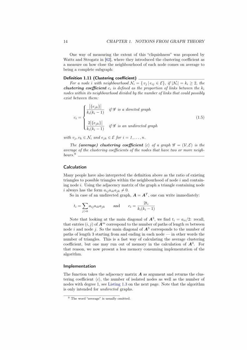
The function takes the adjacency matrix A as argument and returns the clus-tering coefficient 〈c〉, the number of isolated nodes as well as the number ofnodes with degree 1, see Listing 1.3 on the next page. Note that the algorithmis only intended for undirected graphs.
9 The word “average” is usually omitted.
1.4. CHARACTERISTIC VALUES 15
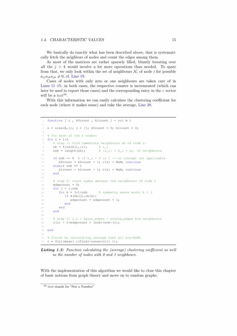
We basically do exactly what has been described above, that is systemati-cally fetch the neighbors of nodes and count the edges among them.
As most of the matrices are rather sparsely filled, bluntly iterating overall the j > k would involve a lot more operations than needed. To sparefrom that, we only look within the set of neighbours Ni of node i for possibleaijaikajk 6= 0, cf. Line 19.
Cases of nodes with only zero or one neighbours are taken care of inLines 11–15: in both cases, the respective counter is incremented (which canlater be used to report those cases) and the corresponding entry in the c vectorwill be a NaN10.
With this information we can easily calculate the clustering coefficient foreach node (where it makes sense) and take the average, Line 28.
1 function [ c , k0count , k1count ] = cc( A )
2
3 n = size(A,1); c = []; k0count = 0; k1count = 0;
4
5 % for each of the n nodes:
6 for i = 1:n
7 % step 1: find immediate neighbours nb of node i:
8 nb = find(A(i,:)); % n_i
9 nnb = length(nb); % |n_i| = k_i = no. of neighbours
10
11 if nnb == 0 % if k_i = 0 or 1 −> cc concept not applicable
12 k0count = k0count + 1; c(i) = NaN; continue
13 elseif nnb == 1
14 k1count = k1count + 1; c(i) = NaN; continue
15 end
16
17 % step 2: count egdes amongst the neighbours of node i
18 edgecount = 0;
19 for j = 1:nnb
20 for k = j+1:nnb % symmetry saves work: k > j
21 if A(nb(j),nb(k))
22 edgecount = edgecount + 1;
23 end
24 end
25 end
26
27 % step 3: c_i = exist_edges / possib_edges b/w neighbours
28 c(i) = 2*edgecount / (nnb*(nnb−1));29
30 end
31
32 % finish by calculating average over all non−NaNs33 c = full(mean( c(find(¬isnan(c))) ));
Listing 1.3: Function calculating the (average) clustering coefficient as wellas the number of nodes with 0 and 1 neighbours.
With the implementation of this algorithm we would like to close this chapterof basic notions from graph theory and move on to random graphs.
10 NaN stands for “Not a Number”

C H A P T E R 2
Random graphs
We introduce three major types of random graphs,
analyse their characteristics and generic properties,
and compare their behaviour with some real world
examples.
2.1 Introduction
As mentioned earlier, the concept of graphs has been around for some centuries.But until the 1950s, attention was paid only to “regular” graphs. In fact, itwas the Hungarians Paul Erdös and Alfréd Réyni who extended the focus onlarge–scale networks with no apparent design principles — “random graphs”.Since their famous paper [19] from 1959, random graph theory has become oneof the main areas of interest in modern discrete mathematics, producing manyand some highly ingenious results. Some of them for instance allow us to betterunderstand the mechanisms that determine or lead to the specific topology ofa large network.
Some dramatic advances have been made in the past few years, mainly madepossible by increases in computational power as well as the computerisation ofdata acquisition in many fields allowing for large databases and abundant dataof various real networks. On the other hand, as boundaries break down betweendifferent disciplines, collaboration of mathematicians, computer experts andbiologists, for example, have brought some interesting advances in systemsbiology, as the classical reductionist modeling approach cannot always give anexplanation for the behaviour of a system as a whole.
In the absence of real data, or for simulation purposes, people tried torecreate the phenomena observed in real networks using random networks. Asa result, a large variety of graph models has been established.
In this chapter we shall review a number of interesting and important find-ings not only for the classical Erdös–Rényi model but also for two other, morerecent models, namely the one by Watts and Strogatz, and the one by Barabásiand Albert. Especially the last model of these will be used extensively in ourlater work.
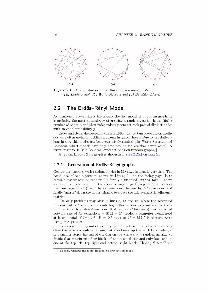
For a first, uncommented impression, Figure 2.1 on the following page showsthree small graphs with 20 nodes and 20 edges created using those models.Larger examples are can be found in Figure 2.2, Figure 2.5 and Figure 2.8 onpages 21, 27 and 33 respectively, each of them having n = 100 nodes and aboute = 200 edges.
17
18 CHAPTER 2. RANDOM GRAPHS
(a) (b) (c)
Figure 2.1: Small instances of our three random graph models:(a) Erdös–Rényi, (b) Watts–Strogatz and (c) Barabási–Albert.
2.2 The Erdös–Rényi Model
As mentioned above, this is historically the first model of a random graph. Itis probably the most natural way of creating a random graph: choose (fix) anumber of nodes n and then independently connect each pair of distinct nodeswith an equal probability p.
Erdös and Rényi discovered in the late 1940s that certain probabilistic meth-ods were often useful in tackling problems in graph theory. Due to its relativelylong history this model has been extensively studied (the Watts–Strogatz andBarabási–Albert models have only been around for less than seven years). Auseful resource is Béla Bollobás’ excellent book on random graphs, [11].
A typical Erdös–Rényi graph is shown in Figure 2.2(a) on page 21.
2.2.1 Generation of Erdös–Rényi graphs
Generating matrices with random entries in Matlab is usually very fast. Thebasic idea of our algorithm, shown in Listing 2.1 on the facing page, is tocreate a matrix with all random (uniformly distributed) entries, take — as wewant an undirected graph — the upper triangular part1, replace all the entriesthat are larger than (1 − p) by true–entries, the rest by false–entries, andfinally “mirror” down the upper triangle to create the full, symmetric adjacencymatrix.
The only problems may arise in lines 8, 13 and 16, where the generatedrandom matrix R can become quite large, thus memory consuming, as it is afull matrix with n2 double–entries (that require 23 bits each). For a desirednetwork size of for example n = 8192 = 213 nodes a computer would needat least a total of 213 · 213 · 23 = 229 bytes or 29 = 512 MB of memory to(temporarily) store R.
To prevent running out of memory even for relatively small n, we not onlyclear the variables right after use, but also break up the work by dividing itinto smaller steps: instead of working on the whole n × n random matrix, wedivide that matrix into four blocks of about equal size and only look one byone at the top left, top right and bottom right block. Having “filtered” the
1 That is, without the main diagonal to prevent self–loops
2.2. THE ERDÖS–RÉNYI MODEL 19
indices of where to place edges, we create them, Line 22, and then finally addthe transpose.
The reason for using the memory consuming method of first generating thesesometimes rather big random matrices is, that it appears to be significantlyfaster than using nested loops, randomly deciding for each entry, one by one,if there should be an edge or not.2
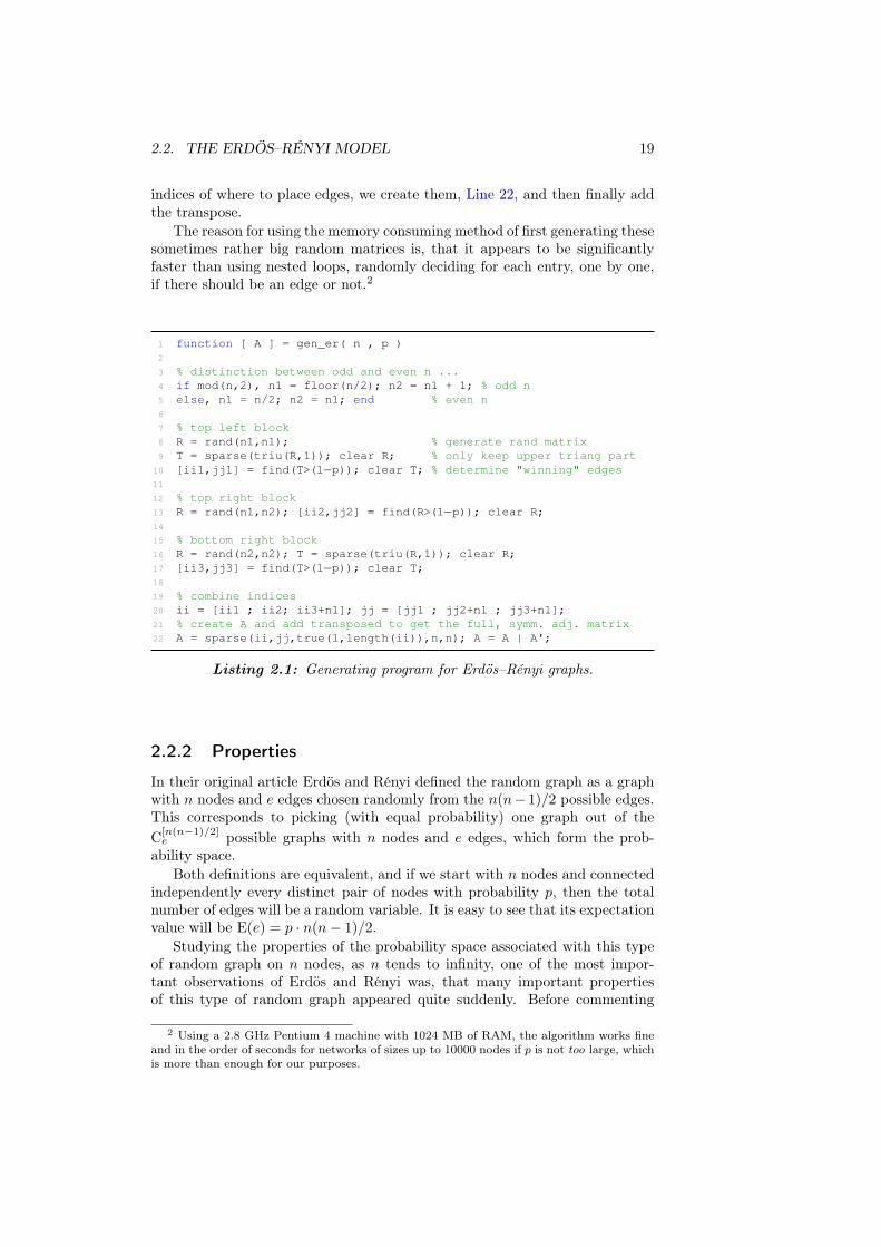
1 function [ A ] = gen_er( n , p )
2
3 % distinction between odd and even n ...
4 if mod(n,2), n1 = floor(n/2); n2 = n1 + 1; % odd n
5 else, n1 = n/2; n2 = n1; end % even n
6
7 % top left block
8 R = rand(n1,n1); % generate rand matrix
9 T = sparse(triu(R,1)); clear R; % only keep upper triang part
10 [ii1,jj1] = find(T>(1−p)); clear T; % determine "winning" edges
11
12 % top right block
13 R = rand(n1,n2); [ii2,jj2] = find(R>(1−p)); clear R;
14
15 % bottom right block
16 R = rand(n2,n2); T = sparse(triu(R,1)); clear R;
17 [ii3,jj3] = find(T>(1−p)); clear T;
18
19 % combine indices
20 ii = [ii1 ; ii2; ii3+n1]; jj = [jj1 ; jj2+n1 ; jj3+n1];
21 % create A and add transposed to get the full, symm. adj. matrix
22 A = sparse(ii,jj,true(1,length(ii)),n,n); A = A | A';
Listing 2.1: Generating program for Erdös–Rényi graphs.
2.2.2 Properties
In their original article Erdös and Rényi defined the random graph as a graphwith n nodes and e edges chosen randomly from the n(n− 1)/2 possible edges.This corresponds to picking (with equal probability) one graph out of theC
[n(n−1)/2]e possible graphs with n nodes and e edges, which form the prob-
ability space.Both definitions are equivalent, and if we start with n nodes and connected
independently every distinct pair of nodes with probability p, then the totalnumber of edges will be a random variable. It is easy to see that its expectationvalue will be E(e) = p · n(n− 1)/2.
Studying the properties of the probability space associated with this typeof random graph on n nodes, as n tends to infinity, one of the most impor-tant observations of Erdös and Rényi was, that many important propertiesof this type of random graph appeared quite suddenly. Before commenting
2 Using a 2.8 GHz Pentium 4 machine with 1024 MB of RAM, the algorithm works fineand in the order of seconds for networks of sizes up to 10000 nodes if p is not too large, whichis more than enough for our purposes.
20 CHAPTER 2. RANDOM GRAPHS
on this however, we would like to present the list of characteristic values forErdös–Rényi graphs.
Characteristic values
As mentioned above, we limit ourselves to presenting the results, but givereferences for further reading.
Degree distribution It is relatively straightforward to show3 that the distribu-tion is binomial:
p(k) = Ckn−1p
k(1− p)n−1−k (2.1)
For large n this distribution can be approximated by a Poisson distribu-tion
p(k) ≃ e〈k〉〈k〉kk!
A typical degree distribution is shown in Figure 2.2(b).
Average node degree Using the expectation value from Subsection 2.2.2:
〈k〉 = 2e/n = p · (n− 1) ≃ pn
Average path length Can be found in [23]:
〈l〉 =lnn− γ
ln(pn)+
1
2
where γ is the Euler–Mascheroni constant, see List of Symbols
Diameter More details in [15], but usually concentrated on a few values around
d ≈ lnn
ln(pn)=
lnn
ln〈k〉
Clustering coefficient For each node, the probability that its neighbours areconnected equals p, so it follows immediately that
〈c〉 = p =〈k〉n
3 It is made up of three parts: the number of possibilities of choosing k nodes out of(n − 1) other nodes (as link–targets), the probability of a particular node actually having k
edges attached to it as well as the probability of not having (n− 1− k) edges attached to it.
2.2. THE ERDÖS–RÉNYI MODEL 21
(a)
Node Degree GGGGGGGGGGA
Fractio
nofnodes
in%
GGGGGGGGGGA
0 2 4 6 8 10 12 140
2
4
6
8
10
12
14
16
18
20
(b)
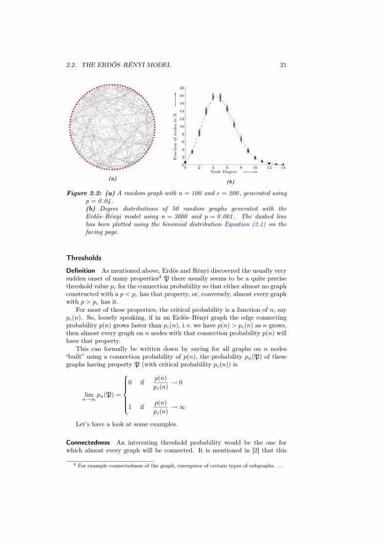
Figure 2.2: (a) A random graph with n = 100 and e = 200 , generated usingp = 0 .04 .(b) Degree distributions of 50 random graphs generated with theErdös–Rényi model using n = 3000 and p = 0 .001 . The dashed linehas been plotted using the binomial distribution Equation (2.1) on thefacing page.
Thresholds
Definition As mentioned above, Erdös and Rényi discovered the usually verysudden onset of many properties4 P there usually seems to be a quite precisethreshold value pc for the connection probability so that either almost no graphconstructed with a p < pc has that property, or, conversely, almost every graphwith p > pc has it.
For most of these properties, the critical probability is a function of n, saypc(n). So, loosely speaking, if in an Erdös–Rényi graph the edge connectingprobability p(n) grows faster than pc(n), i. e. we have p(n) > pc(n) as n grows,then almost every graph on n nodes with that connection probability p(n) willhave that property.
This can formally be written down by saying for all graphs on n nodes“built” using a connection probability of p(n), the probability pn(P) of thesegraphs having property P (with critical probability pc(n)) is
limn→∞
pn(P) =
0 ifp(n)
pc(n)→ 0
1 ifp(n)
pc(n)→∞
Let’s have a look at some examples.
Connectedness An interesting threshold probability would be the one forwhich almost every graph will be connected. It is mentioned in [2] that this
4 For example connectedness of the graph, emergence of certain types of subgraphs, . . .

22 CHAPTER 2. RANDOM GRAPHS
is usually the case if 〈k〉 ≥ lnn, resulting in pc ≈ lnn/n, but a more rigorousapproach gives the following theorem, found in [11]:
Theorem 2.1 (Connectedness of Erdös–Rényi graphs)Let c ∈ R be fixed and let Gn,p(n) be an Erdös–Rényi random graph on n
nodes created using
p(n) =ln(n) + c + o(1 )
n(2.2)
Then the probability pconn that Gn,p(n) is connected tends to
pconn
(
Gn,p(n)
) n→∞−−−−→ e−e−c
(2.3)
where e stands for Euler’s number, e = exp(1 ).
Proof: Also given in [11]. �
Subgraphs Another set of connection probability thresholds can be foundin [2]. There we find, for example, that if we build Erdös–Rényi graphs withn nodes and scale the connection probability used according to p(n) = cn−k/l
with a sensibly chosen c ∈ R, many critical probabilities can be established(proofs of which, again, for example in [11]).
z −∞ −2 − 32 − 4
3 − 54 −1 − 2
3− 1
2
Figure 2.3: Threshold probabilities for the appearance of different types ofsubgraphs for pc(n) ∼ nz . Courtesy of [2].
Just to name a few: in order for almost every graph to contain at least one
– subgraph with k nodes and l edges: pc(n) = cn−k/l
– tree of order k: pc(n) = cn−k/(k−1)
– cycle of length k: pc(n) = cn−1
– complete subgraph on k nodes: pc(n) = cn−2/(k−1)
Some of these are shown in Figure 2.3.
Giant cluster It is intuitive that, for low probabilities, Erdös–Rényi graphsconsist of just a few, isolated edges, sparsely distributed throughout the graph.Increasing p, one witnesses the emergence of tress, cycles and other types ofsubgraphs, but which are still small and isolated clusters.
For p(n) = cn−1, it follows immediately that the average node degree 〈k〉 isconstant. While for c < 1, the graph consists of isolated clusters, a giant cluster

2.3. THE WATTS–STROGATZ OR “SMALL–WORLD” MODEL 23
(clearly distinguishable by it’s size, containing at least about n2/3 nodes) startsto form for values of c ≥ 1.
This phenomenon — passing from a fragmented system to a graph whichis dominated by a single giant cluster, the transition roughly happening atpc(n) ≃ 1/n — is similar to a transition in infinite–dimensional percolation, atopic thoroughly studied, not only in mathematics [27].
With these remarks we would like to move on to a more recent random graphmodel, namely the Watts–Strogatz model.
2.3 The Watts–Strogatz or “small–world”
Model
In the late 1960s, the famous American psychologist Stanley Milgram pro-claimed his thesis about the “six degrees of separation” between any two per-sons in the USA, meaning, that any two randomly chosen individuals are linkedby a chain of six or fewer first–name acquaintances [44].
Social networks indeed have been shown to feature — despite their large net-work size and sparse connections — short average path lengths (which coinedthe term “small–world”), but are still highly clustered. For instance, everybodyhas a local circle of friends, acquaintances through family, education, work orhobbies. Furthermore, we also have a few “long range connections” through rel-atives that moved abroad, an extended stay in an overseas country or somebodyfrom china you got to know in your favoured café.
To see both these features of “clusteredness” and short average path lengthsin Erdös–Rényi graphs, cf. Subsection 2.2.2 on page 20, one would need massiveamounts of edges, as there is little order among them. In the real world however,only relatively few edges are needed for both these characteristics. In 1999,Watts and Strogatz defined this small–world concept [62], showed that manyreal networks have small–world characteristics and introduced an algorithm fortheir creation.
Before describing this algorithm and studying the characteristics of thegraphs generated with it, it is important to mention that the small–worldcharacter can also be found in other types of networks, for example in scale–freegraphs which we will present in Section 2.4 on page 28.
A typical small–world graph is shown in Figure 2.5(a).
2.3.1 Generation of small–world graphs
The idea The idea behind generating graphs with small–world character isquite simple and, on second though, also quite intuitive: start with order andrandomize a bit. Starting off with order allows for the relatively high clustering,yet randomizing by rewiring some edges creates “long distance shortcuts” whichare responsible for the relatively low average path length.
Watts and Strogatz chose a one dimensional lattice with a periodic boundingcondition as starting point: take n nodes, lay them out to form a “ring” andconnect each node with its k0 neighbours. In order for that lattice to besymmetrical, k0 must be even (for example two nodes to the “left” and twonodes to the “right” would mean k0 = 4). Once this regular lattice is generated,
24 CHAPTER 2. RANDOM GRAPHS
pr = 0 −−−−−−−−−−−−−−−−−−−−−−−−−−−−−−−−−−→increasing randomness
pr = 1
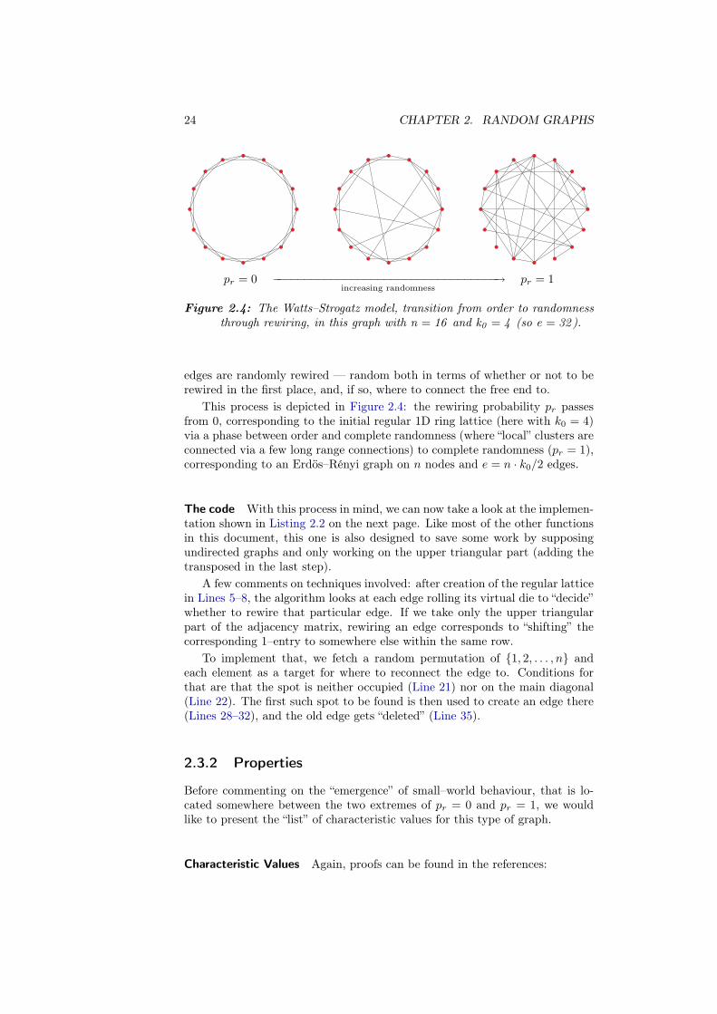
Figure 2.4: The Watts–Strogatz model, transition from order to randomnessthrough rewiring, in this graph with n = 16 and k0 = 4 (so e = 32 ).
edges are randomly rewired — random both in terms of whether or not to berewired in the first place, and, if so, where to connect the free end to.
This process is depicted in Figure 2.4: the rewiring probability pr passesfrom 0, corresponding to the initial regular 1D ring lattice (here with k0 = 4)via a phase between order and complete randomness (where “local” clusters areconnected via a few long range connections) to complete randomness (pr = 1),corresponding to an Erdös–Rényi graph on n nodes and e = n · k0/2 edges.
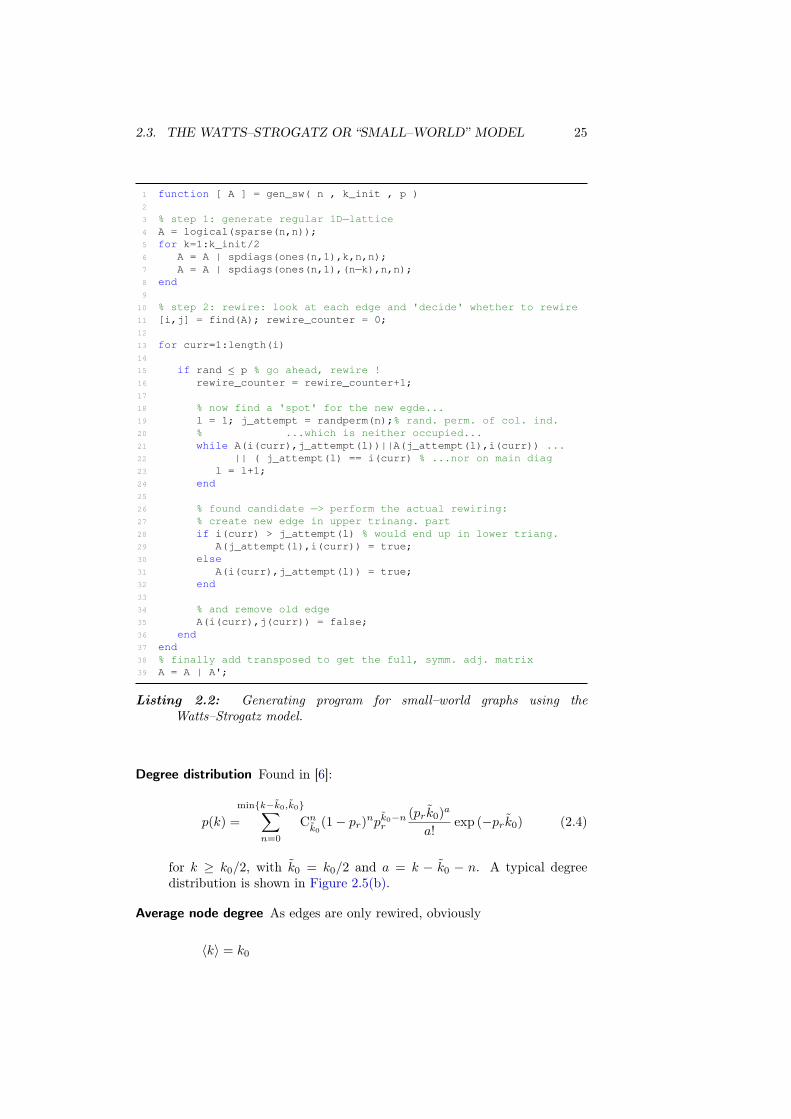
The code With this process in mind, we can now take a look at the implemen-tation shown in Listing 2.2 on the next page. Like most of the other functionsin this document, this one is also designed to save some work by supposingundirected graphs and only working on the upper triangular part (adding thetransposed in the last step).
A few comments on techniques involved: after creation of the regular latticein Lines 5–8, the algorithm looks at each edge rolling its virtual die to “decide”whether to rewire that particular edge. If we take only the upper triangularpart of the adjacency matrix, rewiring an edge corresponds to “shifting” thecorresponding 1–entry to somewhere else within the same row.
To implement that, we fetch a random permutation of {1, 2, . . . , n} andeach element as a target for where to reconnect the edge to. Conditions forthat are that the spot is neither occupied (Line 21) nor on the main diagonal(Line 22). The first such spot to be found is then used to create an edge there(Lines 28–32), and the old edge gets “deleted” (Line 35).
2.3.2 Properties
Before commenting on the “emergence” of small–world behaviour, that is lo-cated somewhere between the two extremes of pr = 0 and pr = 1, we wouldlike to present the “list” of characteristic values for this type of graph.
Characteristic Values Again, proofs can be found in the references:
2.3. THE WATTS–STROGATZ OR “SMALL–WORLD” MODEL 25
1 function [ A ] = gen_sw( n , k_init , p )
2
3 % step 1: generate regular 1D−lattice4 A = logical(sparse(n,n));
5 for k=1:k_init/2
6 A = A | spdiags(ones(n,1),k,n,n);
7 A = A | spdiags(ones(n,1),(n−k),n,n);8 end
9
10 % step 2: rewire: look at each edge and 'decide' whether to rewire
11 [i,j] = find(A); rewire_counter = 0;
12
13 for curr=1:length(i)
14
15 if rand ≤ p % go ahead, rewire !
16 rewire_counter = rewire_counter+1;
17
18 % now find a 'spot' for the new egde...
19 l = 1; j_attempt = randperm(n);% rand. perm. of col. ind.
20 % ...which is neither occupied...
21 while A(i(curr),j_attempt(l))||A(j_attempt(l),i(curr)) ...
22 || ( j_attempt(l) == i(curr) % ...nor on main diag
23 l = l+1;
24 end
25
26 % found candidate −> perform the actual rewiring:
27 % create new edge in upper trinang. part
28 if i(curr) > j_attempt(l) % would end up in lower triang.
29 A(j_attempt(l),i(curr)) = true;
30 else
31 A(i(curr),j_attempt(l)) = true;
32 end
33
34 % and remove old edge
35 A(i(curr),j(curr)) = false;
36 end
37 end
38 % finally add transposed to get the full, symm. adj. matrix
39 A = A | A';
Listing 2.2: Generating program for small–world graphs using theWatts–Strogatz model.
Degree distribution Found in [6]:
p(k) =
min{k−k0,k0}∑
n=0
Cnk0
(1− pr)npk0−n
r
(prk0)a
a!exp (−prk0) (2.4)
for k ≥ k0/2, with k0 = k0/2 and a = k − k0 − n. A typical degreedistribution is shown in Figure 2.5(b).
Average node degree As edges are only rewired, obviously
〈k〉 = k0
26 CHAPTER 2. RANDOM GRAPHS
Average path length To the best of our knowledge, an exact solution has notbe found yet. In [49] however, we find a good approximation for a modelvery similar to the one discussed here. The only difference is that insteadof rewiring edges, shortcuts are added directly (thus leaving the originalring lattice “intact”, but increasing the total number of edges).5 There,
〈l〉 ≃ ξ
k0
√
1 + 2ξ/ntanh−1
(
1√
1 + 2ξ/n
)
(2.5)
where ξ = 2/(k0ps) with ps is the probability similar to the Erdös–Rényimodel of having a shortcut between two nodes.
Diameter Again, to the best of our knowledge no firm analytic results areavailable at the time of writing.
Clustering coefficient A slightly different but equivalent definition of the clus-tering coefficient than that given in Subsection 1.4.4 would be to define itas the fraction of the mean number of edges between the neighbours of anode and the mean number of possible edges between those neighbours.
For this definition of clustering, we find in [6]:
〈c〉′ = 〈c〉′0(1− p)3 =3(k0/2− 1)
2(k0 − 1)(1− p)3
and the deviation from 〈c〉 is of order 1/n. So we can readily say
〈c〉 ≃ 〈c〉0(1− p)3 (2.6)
the index 0 denoting, again, the value for pr = 0.6
Influence of the rewiring probability As we have mentioned earlier on, typicalsmall–world graphs show a remarkable combination of high clustering (whichis a local property) and short average path lengths (a global measure).
In order to stick closely to properties of some real networks (like socialnetworks), Watts and Strogatz were interested in graphs with many verticesbut few connections between them (but not so few that the graph would be indanger of becoming disconnected). They specified their request by demanding
n≫ k0 ≫ lnn≫ 1
Here, k ≫ lnn guarantees that the resulting graph will be connected, [10].With their model (and appropriately chosen parameters fulfilling this request)it is easy to obtain the desired high clustering and short distances. Again,an Erdös–Rényi graph with similar properties would need to have significantlymore edges.
However, even with the Watts–Strogatz model the desired properties arenot always present. In fact, the emergence of this behaviour depends stronglyon pr. If we look at both extremes, we find
5 Both models are equivalent for sufficiently small pr respectively ps and large n.6 It can easily be established that 〈c〉0 =
3(k0−2)4(k0−1)
.
2.3. THE WATTS–STROGATZ OR “SMALL–WORLD” MODEL 27
(a)
Node Degree GGGGGGGGGGA
Fractio
nofnodes
in%
GGGGGGGGGGA
0 1 2 3 4 5 6 7 80
10
20
30
40
50
60
70
80
90
100
(b)
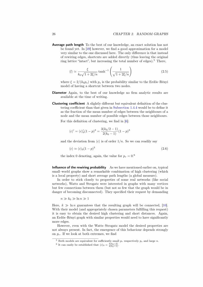
Figure 2.5: (a) A small–world graph with n = 100 and e = 200 , generatedwith the Watts–Strogatz model using pr = 0 .05 and k0 = 4 .(b) Degree distributions of 50 small–world graphs generated usingn = 3000 , k0 = 6 and pr = 0 .01 . The dashed line has been plotted us-ing the distribution Equation (2.4) on page 25.
〈c〉0 =3(k0 − 2)
4(k0 − 1)≃ 3
4GGGGGGGGGGGGGGGGGGA 〈c〉1 ∼
k0
n0→pr→1
〈l〉0 =n(n + k0 − 2)
2k0(n− 1)≃ n
2k0GGGGGGGGGGGA 〈l〉1 ∼
lnn
ln(k0 − 1)
thus for small pr, 〈c〉 seems to be large and 〈l〉 scales linearly with n, whereasfor large pr the clustering coefficient seems to decrease with the system sizeand the average path length only scales logarithmically with n.
Both these extremes and intuition seem to suggest that a large 〈c〉 is alwaysassociated with a large 〈l〉, and small clustering with short path lengths.
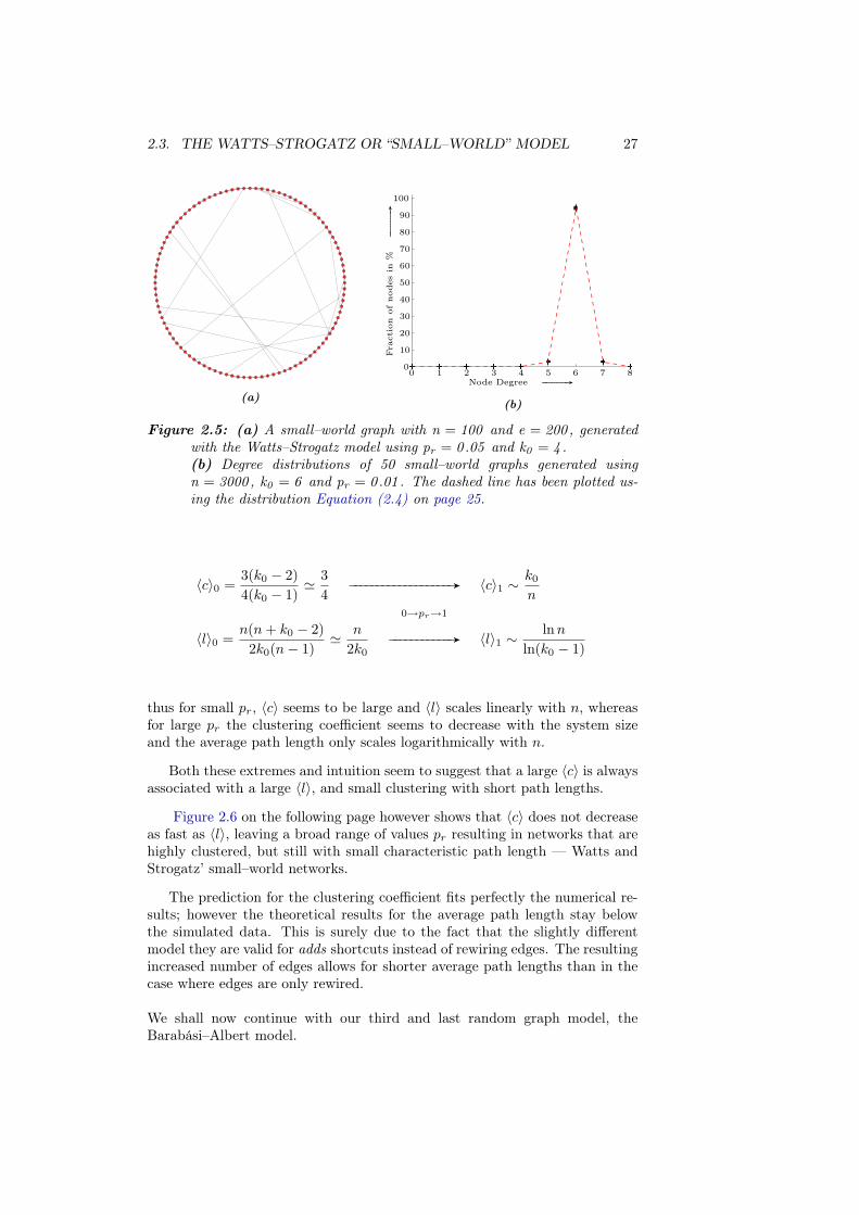
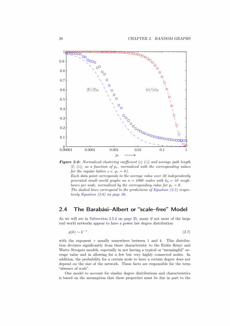
Figure 2.6 on the following page however shows that 〈c〉 does not decreaseas fast as 〈l〉, leaving a broad range of values pr resulting in networks that arehighly clustered, but still with small characteristic path length — Watts andStrogatz’ small–world networks.
The prediction for the clustering coefficient fits perfectly the numerical re-sults; however the theoretical results for the average path length stay belowthe simulated data. This is surely due to the fact that the slightly differentmodel they are valid for adds shortcuts instead of rewiring edges. The resultingincreased number of edges allows for shorter average path lengths than in thecase where edges are only rewired.
We shall now continue with our third and last random graph model, theBarabási–Albert model.
28 CHAPTER 2. RANDOM GRAPHS
pr GGGGGGA
〈l〉/〈l〉0 〈c〉/〈c〉0
0.00001 0.0001 0.001 0.01 0.1 10
0.1
0.2
0.3
0.4
0.5
0.6
0.7
0.8
0.9
1
Figure 2.6: Normalized clustering coefficient 〈c〉 (�) and average path length〈l〉 (�), as a function of pr, normalized with the corresponding valuesfor the regular lattice i. e. pr = 0 ).Each data point corresponds to the average value over 50 independentlygenerated small–world graphs on n = 1000 nodes with k0 = 10 neigh-bours per node, normalized by the corresponding value for pr = 0 .The dashed lines correspond to the predictions of Equation (2.5) respec-tively Equation (2.6) on page 26.
2.4 The Barabási–Albert or “scale–free” Model
As we will see in Subsection 2.5.2 on page 35, many if not most of the largereal world networks appear to have a power law degree distribution
p(k) ∼ k−γ (2.7)
with the exponent γ usually somewhere between 1 and 4. This distribu-tion deviates significantly from those characteristic to the Erdös–Rényi andWatts–Strogatz models, especially in not having a typical or “meaningful” av-erage value and in allowing for a few but very highly connected nodes. Inaddition, the probability for a certain node to have a certain degree does notdepend on the size of the network. These facts are responsible for the term“absence of scale”.
One model to account for similar degree distributions and characteristicsis based on the assumption that these properties must be due in part to the
2.4. THE BARABÁSI–ALBERT OR “SCALE–FREE” MODEL 29
evolution inherent to certain types of networks: on one hand they usuallyshow some sort of growth, and, on the other hand, new nodes introduced intothe network usually connect preferentially to the more highly connected nodesalready present in the network. This non uniform connection probability seemsto introduce certain correlations and dependences that allow for some of thespecific attributes of these graphs.
In addition, as the power law degree distribution allows for some (very fewbut) extremely high node degrees, many real world networks have a certainmaximum node degree, or cutoff, that limits or bounds the range of nodedegrees. Here, the plot of the degree distribution deviates from a straight linein a double logarithmic plot to show an exponential or “Gaussian” tail. Amaralet al. give a more detailed introduction to these phenomena, [3].
Building a suitable model for these types of networks has been an areaof high interest in the past few years and a multitude of models has sincearisen. Table III in [2] gives an excellent overview of the overwhelming numberof variations on the model. In this paper however, we will limit ourselves tothe seminal Barabási–Albert model, which gave rise to the burst of activity inthe field. A typical scale–free graph generated with their model is shown inFigure 2.8(a).
2.4.1 Generation of scale–free graphs
The idea Although it is straightforward to generate networks with a specificdegree distribution (just by generating node degrees according to the specificdistribution and then randomly placing the edges accordingly), until lately,those networks failed to show key properties observed in real world networkswith a power law distribution.
One reason for this was that the usual generating method did not reflectthe dynamical process that creates real world networks, introducing nontrivialcorrelations that affect many topological properties. Seeing the evolution ofreal world networks (like the world wide web, which started with a coupleof hundred pages, and now has grown to many billion pages), the generatingalgorithm for an artificial network should also incorporate a similar growthprocess as well as the preferential attachment (as, for example, some new pageis much more likely to link to an important page like www.google.com than tosome rather insignificant page).
Both ideas inspired the first model introduced by Barabási et al. in 1999, [4],which generated a scale–free network with a power law degree distribution andmany of the properties encountered in real networks. This model allowed forthe first time to describe the inherent ordering principle observed in real worldnetworks. Its simple but elegant generating algorithm is the following:
(i) Growth: Start with a very small but fully connected graph on n0 nodes(1 ≤ n0 ≪ n, n being the desired final number of nodes). At eachiteration step t, add one node with m edges that link the new node to mnodes that already are in the system.
(ii) Preferential attachment : The “targets” for the m new edges to be placedare not chosen with equal probability, but with probability proportional
30 CHAPTER 2. RANDOM GRAPHS
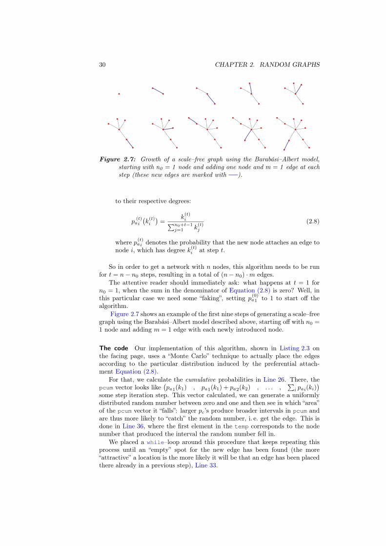
Figure 2.7: Growth of a scale–free graph using the Barabási–Albert model,starting with n0 = 1 node and adding one node and m = 1 edge at eachstep (these new edges are marked with ).
to their respective degrees:
pa(t)i
(
k(t)i
)
=k
(t)i
∑n0+t−1j=1 k
(t)j
(2.8)
where pa(t)i denotes the probability that the new node attaches an edge to
node i, which has degree k(t)i at step t.
So in order to get a network with n nodes, this algorithm needs to be runfor t = n− n0 steps, resulting in a total of (n− n0) ·m edges.
The attentive reader should immediately ask: what happens at t = 1 forn0 = 1, when the sum in the denominator of Equation (2.8) is zero? Well, inthis particular case we need some “faking”, setting pa
(0)1 to 1 to start off the
algorithm.Figure 2.7 shows an example of the first nine steps of generating a scale–free
graph using the Barabási–Albert model described above, starting off with n0 =1 node and adding m = 1 edge with each newly introduced node.
The code Our implementation of this algorithm, shown in Listing 2.3 onthe facing page, uses a “Monte Carlo” technique to actually place the edgesaccording to the particular distribution induced by the preferential attach-ment Equation (2.8).
For that, we calculate the cumulative probabilities in Line 26. There, thepcum vector looks like
(
pa1(k1) , pa1(k1) + pa2(k2) , . . . ,∑
i pai(ki))
some step iteration step. This vector calculated, we can generate a uniformlydistributed random number between zero and one and then see in which “area”of the pcum vector it “falls”: larger pc’s produce broader intervals in pcum andare thus more likely to “catch” the random number, i. e. get the edge. This isdone in Line 36, where the first element in the temp corresponds to the nodenumber that produced the interval the random number fell in.
We placed a while–loop around this procedure that keeps repeating thisprocess until an “empty” spot for the new edge has been found (the more“attractive” a location is the more likely it will be that an edge has been placedthere already in a previous step), Line 33.
2.4. THE BARABÁSI–ALBERT OR “SCALE–FREE” MODEL 31
Finally, in order to create a network with n nodes, n − n0 repetitions areneeded (Line 15), within each of which m edge–placement–runs need to becarried out (Line 30).
2.4.2 Properties
Now that we are able to generate the basic type of scale–free networks, let’stake a closer look at their properties, starting off with the characteristic values.
Characteristic Values Again, proofs can be found in the references:
Degree distribution Found in [2]
p(k) =2m(m + 1)
k(k + 1)(k + 2)∼ k−3 (2.9)
A typical degree distribution is shown in Figure 2.8(b).
Average node degree Straightforward:
〈k〉 = 2e/n =2m(n− no)
n≃ 2m
Average path length In [23] it is shown that in a good approximation
〈l〉 ≃ lnn− ln(m/2)− 1− γ
ln(ln n) + ln(m/2)+
3
2(2.10)
Diameter Using a similar model, with the difference of allowing for multipleedges and self loops, we find in [12] for very large n and m ≥ 2 that d isusually concentrated on a few values around
d ≈ lnn
ln(ln n)
For m = 1 it is shown in the same paper that d scales as lnn.
Clustering coefficient We find in [22]:
〈c〉 =6m2
[
(m + 1)2(ln t)2 − 8m ln t + 8m]
8(m− 1)(6m2 + 8m + 3)t
Ultra small–world If we take a look at Equation (2.10), we can see that forlarge n the average path length scales as lnn/ ln(ln n), which increases muchmore slowly than lnn, a suggested asymptotic form for graphs generated byboth the Watts–Strogatz and Erdös–Rényi model, see for example [49].
Besides an alternative way of finding the approximation 〈l〉 ∼ lnn/ ln(ln n),it is claimed in [16] that scale–free networks are “ultrasmall”. In Figure 2.9on page 34 we compare the growth of 〈l〉 as n increases. To make the graphscomparable, the respective generating parameters have been chosen in a waythat for each graph e ≃ 4n. This relatively high number of edges is needed
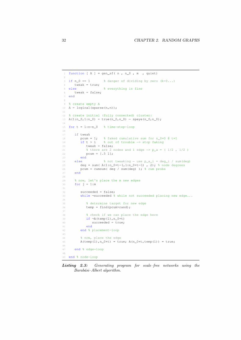
32 CHAPTER 2. RANDOM GRAPHS
1 function [ A ] = gen_sf( n , n_0 , m , quiet)
2
3 if n_0 == 1 % danger of dividing by zero (k=0...)
4 tweak = true;
5 else % everything is fine
6 tweak = false;
7 end
8
9 % create empty A
10 A = logical(sparse(n,n));
11
12 % create initial (fully connected) cluster:
13 A(1:n_0,1:n_0) = true(n_0,n_0) − speye(n_0,n_0);
14
15 for t = 1:n−n_0 % time−step−loop16
17 if tweak
18 pcum = 1; % faked cumulative sum for n_0=0 @ t=1
19 if t > 1 % out of trouble −> stop faking
20 tweak = false;
21 % there are 2 nodes and 1 edge −> p_a = ( 1/2 , 1/2 )
22 pcum = [.5 1];
23 end
24 else % not tweaking − use p_a_i = deg_i / sum(deg)
25 deg = sum( A(1:n_0+t−1,1:n_0+t−1) , 2); % node degrees
26 pcum = cumsum( deg / sum(deg) ); % cum probs
27 end
28
29 % now, let's place the m new edges
30 for j = 1:m
31
32 succeeded = false;
33 while ¬succeeded % while not succeeded placing new edge...
34
35 % determine target for new edge
36 temp = find(pcum>rand);
37
38 % check if we can place the edge here
39 if ¬A(temp(1),n_0+t)40 succeeded = true;
41 end
42 end % placement−loop43
44 % now, place the edge
45 A(temp(1),n_0+t) = true; A(n_0+t,temp(1)) = true;
46
47 end % edge−loop48
49 end % node−loop
Listing 2.3: Generating program for scale–free networks using theBarabási–Albert algorithm.
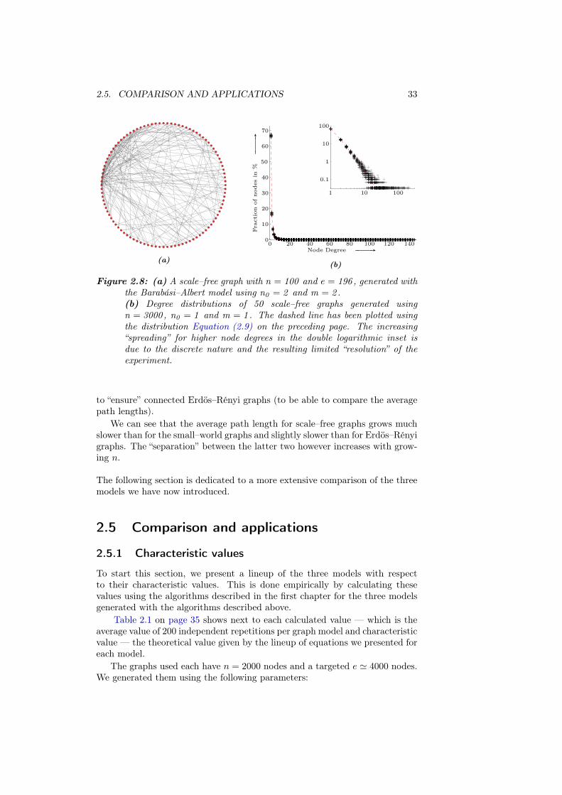
2.5. COMPARISON AND APPLICATIONS 33
(a)
Node Degree GGGGGGGGGGA
Fractio
nofnodes
in%
GGGGGGGGGGA
1 10 100
0 20 40 60 80 100 120 140
0.1
1
10
100
0
10
20
30
40
50
60
70
(b)
Figure 2.8: (a) A scale–free graph with n = 100 and e = 196 , generated withthe Barabási–Albert model using n0 = 2 and m = 2 .(b) Degree distributions of 50 scale–free graphs generated usingn = 3000 , n0 = 1 and m = 1 . The dashed line has been plotted usingthe distribution Equation (2.9) on the preceding page. The increasing“spreading” for higher node degrees in the double logarithmic inset isdue to the discrete nature and the resulting limited “resolution” of theexperiment.
to “ensure” connected Erdös–Rényi graphs (to be able to compare the averagepath lengths).
We can see that the average path length for scale–free graphs grows muchslower than for the small–world graphs and slightly slower than for Erdös–Rényigraphs. The “separation” between the latter two however increases with grow-ing n.
The following section is dedicated to a more extensive comparison of the threemodels we have now introduced.
2.5 Comparison and applications
2.5.1 Characteristic values
To start this section, we present a lineup of the three models with respectto their characteristic values. This is done empirically by calculating thesevalues using the algorithms described in the first chapter for the three modelsgenerated with the algorithms described above.
Table 2.1 on page 35 shows next to each calculated value — which is theaverage value of 200 independent repetitions per graph model and characteristicvalue — the theoretical value given by the lineup of equations we presented foreach model.
The graphs used each have n = 2000 nodes and a targeted e ≃ 4000 nodes.We generated them using the following parameters:
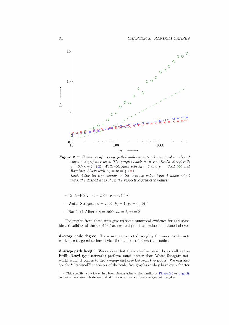
34 CHAPTER 2. RANDOM GRAPHS
n GGGGGGA
〈l〉GGGGGGA
10 100 10000
5
10
15
Figure 2.9: Evolution of average path lengths as network size (and number ofedges e ≃ 4n) increases. The graph models used are: Erdös–Rényi withp = 8/(n − 1 ) (�), Watts–Strogatz with k0 = 8 and pr = 0 .01 (�) andBarabási–Albert with n0 = m = 4 (×).Each datapoint corresponds to the average value from 5 independentruns, the dashed lines show the respective predicted values.
– Erdös–Rényi: n = 2000, p = 4/1998
– Watts–Strogatz: n = 2000, k0 = 4, pr = 0.016 7
– Barabási–Albert: n = 2000, n0 = 2, m = 2
The results from these runs give us some numerical evidence for and someidea of validity of the specific features and predicted values mentioned above:
Average node degree These are, as expected, roughly the same as the net-works are targeted to have twice the number of edges than nodes.
Average path length We can see that the scale–free networks as well as theErdös–Rényi type networks perform much better than Watts–Strogatz net-works when it comes to the average distance between two nodes. We can alsosee the “ultrasmall” character of the scale–free graphs as they have even shorter
7 This specific value for pr has been chosen using a plot similar to Figure 2.6 on page 28to create maximum clustering but at the same time shortest average path lengths.

2.5. COMPARISON AND APPLICATIONS 35
path lengths than the Erdös–Rényi ones. The predicted values are also quite inagreement with the numerical results (but for deviation in the Watts–Strogatzmodel), as we could also see in Figure 2.9.
Diameter These values are unfortunately relatively different from their pre-dictions, or even undetermined as in the Watts–Strogatz case. Concerningthe deviations, however, the values are still in accordance with the boundssurrounding them (see [15] and [12] for further details).
Clustering coefficient As expected, clustering is much higher in small–worldnetworks than in the others. As we mentioned earlier in the introduction tothe Watts–Strogatz model, the scale–free graphs also shows some small–worldbehaviour, as their clustering coefficient is still about 8 times higher than thatof a random graph. For every graph model, prediction and simulation agreevery well.
ValueErdös–Rényi Watts–Strogatz Barabási–Albert
num. theor. num. theor. num. theor.
〈k〉 4.001 4.000 4.000 4.000 3.996 3.996〈l〉 5.599 5.565 25.549 18.723 4.373 4.470d 11.850 5.481 62.570 ? 7.990 3.748〈c〉 0.002 0.002 0.477 0.476 0.015 0.015
Table 2.1: Comparison of the characteristic values between the three networkmodels as well as between the calculated and theoretical values. Eachof the “numerical” values are the average values gained from 200 in-dependently generated networks having n = 2000 nodes and a targetede = 4000 edges.
2.5.2 The real world
To close this chapter on random graphs we would like to present some examplesof real networks whose characteristics can be particularly well reflected by someof the models presented above.
World wide web and internet The world wide web (as of the network ofweb pages connected by hyperlinks) and also the internet (as of the network ofinterconnected computers, routers, servers, etc.) are the largest networks withquite precisely measurable topological data available today.
In contrast to the internet however, the world wide web is usually approxi-mated by directed graphs, resulting in two degree distributions for web pages— one for in– and another one for the out–degrees of pages. It has been shownin several papers (to name a few [14, 26, 60]) that the internet (on routerand domain level) as well as the world wide web (at domain and page level)has node degrees displaying a clear power law distribution with γ for in– andout–degrees usually between 2.0 and 2.5.
36 CHAPTER 2. RANDOM GRAPHS
Phone call networks Another intuitive network that can be established isthat of phone call patterns, where phone numbers are the nodes, connectedby (directed) arcs representing calls. Studies of long distance calls on a singleday [1] have shown that such graph also has a power law in– and out–degreedistribution with exponent γ ≃ 2.1.
Citation networks A scale free degree distribution can also be found in graphsdescribing citations, nodes being documents and directed edges citations be-tween them. Highly connected nodes would correspond to some few seminalpapers where as larger numbers of less significant papers have only few connec-tions. A study [54] showed that the probability of a paper being cited k timescan be described with a power law, using γ ≃ 3.
Human sexual contacts Based on a Swedish survey from 1996 [40], an inter-esting study [41] shows that the number of sexual partners up to 12 monthsprior to the survey is distributed according to a power law, with exponent ofabout γ ≃ 2.4. Besides that, the data and heuristic explanations show thatthese networks are consistent with the preferential attachment mechanism dis-cussed above.
Collaboration networks Large and publicly available databases like IMDB8
or arXiv.org9 allow close studies of another set of networks that can be estab-lished, namely those capturing collaborations. Here, actors or scientists makeup the nodes, and are linked together if they have starred together in a movierespectively were co–authors of some paper.
Several papers show studies of these networks, [5, 50, 62], and find powerlaw exponents usually around γ = 2.4.
Neural networks and power grids Neural networks like those of small wormsor power grids like those spanning the western United States [3] show similarproperties, namely that the average path lengths are close to those of compa-rable Erdös–Rényi graphs, but clustering is significantly higher.
In [62], when Watts et al. introduced the small–world model, they showedthat the properties of these networks as well as the previous two social networkscan be reflected very well by their model.
Protein folding In general, protein folding can be seen as the process a proteingoes through in order to assume its functional shape or conformation. Asprotein molecules are chains of simple, unbranched amino acids, it is throughcoiling into a certain three–dimensional shape that they perform their specificbiological function.
During that process, the different (consecutive) configurations a proteingoes through can be described with a graph, where each node corresponds toa particular conformation, two nodes being linked together if they can be ob-tained from each other by an elementary move. Several papers show that these
8 That is the Internet Movie Database9 The e–Print archive arXiv.org actually provides free and publicly accessible copies of
the majority of the papers and articles cited in this document.

2.5. COMPARISON AND APPLICATIONS 37
networks show significant small–world characteristics, [53, 55, 61] and typicallyhave scale–free degree distributions.
This biologically motivated topic will actually be treated in more detail inChapter 5. We shall now continue, however, with a number of ranking schemesthat we will use to identify important nodes in a network.

C H A P T E R 3
Ranking schemes
We present methods to rank nodes, including node
degrees, algorithms like HITS and PageRank,
centrality based measures like excentricity, status or
centroid value, and “damage”.
3.1 Introduction
With the necessary terminology that we have gathered in the first chapterwe discussed three major models for random graphs. With these models itis easy to generate graphs of arbitrary size, but also modeling the real worldconfronts us in many cases with large if not gigantic networks. One just hasto think of the snapshot the search engine Google has taken of the internetby indexing more than 8 billion pages and capturing the hyperlinks betweenthese pages, [25]. But also metabolic networks or protein–protein interactionnetworks can currently have several thousand nodes, see Chapter 5.
The sheer size of these graphs makes it quite impossible to analyse them byjust “looking” at them. A much more systematic approach needs to be taken.
In many applications one question almost always arises, and has gotten alot of attention in the last ten years especially in relation with informationretrieval systems like Google:
“How do I find the most ‘important’ nodes in a network?”
Ignoring the actual interpretation of “importance” for the moment, we couldanswer the above question in a detailed and elegant way by establishing aranking of the nodes. This can be done by calculating some sort of “score” foreach node in the network — desirably in a systematic and sensible way.
The actual notion of importance that a ranking scheme attributes to thescores depends, of course, on the actual measure of importance used, and hasto ultimately prove itself in the actual practical application.
Before focusing on that, which is done in the last chapter, we shall firstpresent a variety of classical and more recent measures of importance accom-panied by Matlab implementations of their algorithms.
39
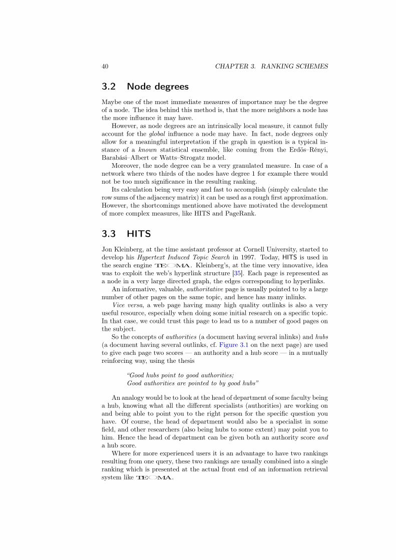
40 CHAPTER 3. RANKING SCHEMES
3.2 Node degrees
Maybe one of the most immediate measures of importance may be the degreeof a node. The idea behind this method is, that the more neighbors a node hasthe more influence it may have.
However, as node degrees are an intrinsically local measure, it cannot fullyaccount for the global influence a node may have. In fact, node degrees onlyallow for a meaningful interpretation if the graph in question is a typical in-stance of a known statistical ensemble, like coming from the Erdös–Rényi,Barabási–Albert or Watts–Strogatz model.
Moreover, the node degree can be a very granulated measure. In case of anetwork where two thirds of the nodes have degree 1 for example there wouldnot be too much significance in the resulting ranking.
Its calculation being very easy and fast to accomplish (simply calculate therow sums of the adjacency matrix) it can be used as a rough first approximation.However, the shortcomings mentioned above have motivated the developmentof more complex measures, like HITS and PageRank.
3.3 HITS
Jon Kleinberg, at the time assistant professor at Cornell University, started todevelop his Hypertext Induced Topic Search in 1997. Today, HITS is used inthe search engine TEOMA. Kleinberg’s, at the time very innovative, ideawas to exploit the web’s hyperlink structure [35]. Each page is represented asa node in a very large directed graph, the edges corresponding to hyperlinks.
An informative, valuable, authoritative page is usually pointed to by a largenumber of other pages on the same topic, and hence has many inlinks.
Vice versa, a web page having many high quality outlinks is also a veryuseful resource, especially when doing some initial research on a specific topic.In that case, we could trust this page to lead us to a number of good pages onthe subject.
So the concepts of authorities (a document having several inlinks) and hubs(a document having several outlinks, cf. Figure 3.1 on the next page) are usedto give each page two scores — an authority and a hub score — in a mutuallyreinforcing way, using the thesis
“Good hubs point to good authorities;Good authorities are pointed to by good hubs”
An analogy would be to look at the head of department of some faculty beinga hub, knowing what all the different specialists (authorities) are working onand being able to point you to the right person for the specific question youhave. Of course, the head of department would also be a specialist in somefield, and other researchers (also being hubs to some extent) may point you tohim. Hence the head of department can be given both an authority score anda hub score.
Where for more experienced users it is an advantage to have two rankingsresulting from one query, these two rankings are usually combined into a singleranking which is presented at the actual front end of an information retrievalsystem like TEOMA.
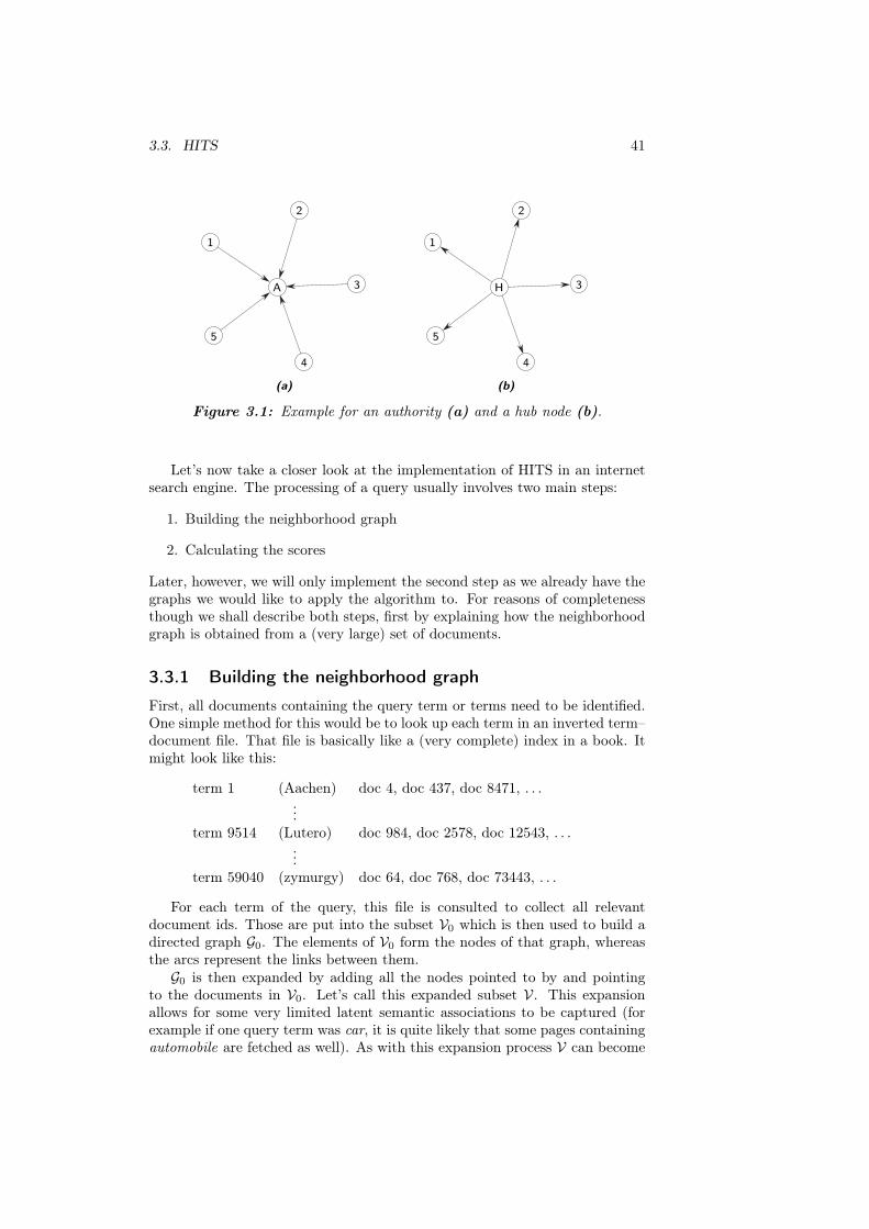
3.3. HITS 41
1
2
3
4
5
A
(a)
1
2
3
4
5
H
(b)
Figure 3.1: Example for an authority (a) and a hub node (b).
Let’s now take a closer look at the implementation of HITS in an internetsearch engine. The processing of a query usually involves two main steps:
1. Building the neighborhood graph
2. Calculating the scores
Later, however, we will only implement the second step as we already have thegraphs we would like to apply the algorithm to. For reasons of completenessthough we shall describe both steps, first by explaining how the neighborhoodgraph is obtained from a (very large) set of documents.
3.3.1 Building the neighborhood graph
First, all documents containing the query term or terms need to be identified.One simple method for this would be to look up each term in an inverted term–document file. That file is basically like a (very complete) index in a book. Itmight look like this:
term 1 (Aachen) doc 4, doc 437, doc 8471, . . ....
term 9514 (Lutero) doc 984, doc 2578, doc 12543, . . ....
term 59040 (zymurgy) doc 64, doc 768, doc 73443, . . .
For each term of the query, this file is consulted to collect all relevantdocument ids. Those are put into the subset V0 which is then used to build adirected graph G0. The elements of V0 form the nodes of that graph, whereasthe arcs represent the links between them.G0 is then expanded by adding all the nodes pointed to by and pointing
to the documents in V0. Let’s call this expanded subset V. This expansionallows for some very limited latent semantic associations to be captured (forexample if one query term was car, it is quite likely that some pages containingautomobile are fetched as well). As with this expansion process V can become
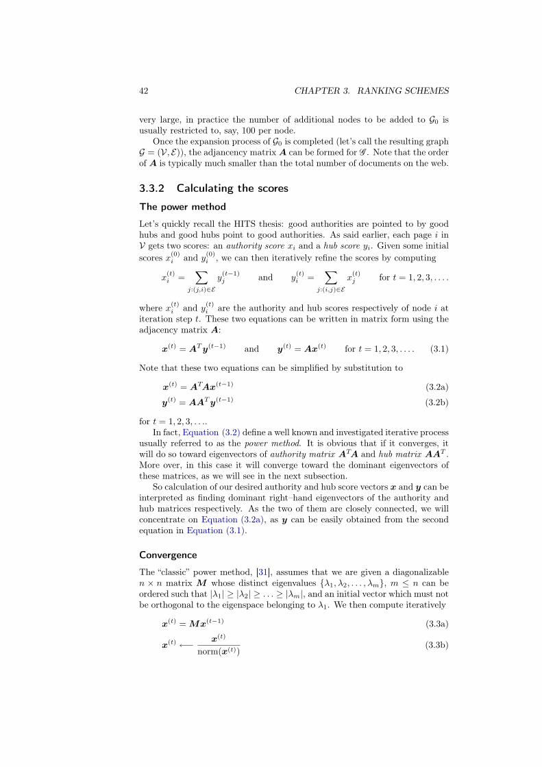
42 CHAPTER 3. RANKING SCHEMES
very large, in practice the number of additional nodes to be added to G0 isusually restricted to, say, 100 per node.
Once the expansion process of G0 is completed (let’s call the resulting graphG = (V, E)), the adjancency matrix A can be formed for G . Note that the orderof A is typically much smaller than the total number of documents on the web.
3.3.2 Calculating the scores
The power method
Let’s quickly recall the HITS thesis: good authorities are pointed to by goodhubs and good hubs point to good authorities. As said earlier, each page i inV gets two scores: an authority score xi and a hub score yi. Given some initialscores x
(0)i and y
(0)i , we can then iteratively refine the scores by computing
x(t)i =
∑
j:(j,i)∈E
y(t−1)j and y
(t)i =
∑
j:(i,j)∈E
x(t)j for t = 1, 2, 3, . . . .
where x(t)i and y
(t)i are the authority and hub scores respectively of node i at
iteration step t. These two equations can be written in matrix form using theadjacency matrix A:
x(t) = AT y(t−1) and y(t) = Ax(t) for t = 1, 2, 3, . . . . (3.1)
Note that these two equations can be simplified by substitution to
x(t) = ATAx(t−1) (3.2a)
y(t) = AAT y(t−1) (3.2b)
for t = 1, 2, 3, . . ..In fact, Equation (3.2) define a well known and investigated iterative process
usually referred to as the power method. It is obvious that if it converges, itwill do so toward eigenvectors of authority matrix ATA and hub matrix AAT .More over, in this case it will converge toward the dominant eigenvectors ofthese matrices, as we will see in the next subsection.
So calculation of our desired authority and hub score vectors x and y can beinterpreted as finding dominant right–hand eigenvectors of the authority andhub matrices respectively. As the two of them are closely connected, we willconcentrate on Equation (3.2a), as y can be easily obtained from the secondequation in Equation (3.1).
Convergence
The “classic” power method, [31], assumes that we are given a diagonalizablen × n matrix M whose distinct eigenvalues {λ1, λ2, . . . , λm}, m ≤ n can beordered such that |λ1| ≥ |λ2| ≥ . . . ≥ |λm|, and an initial vector which must notbe orthogonal to the eigenspace belonging to λ1. We then compute iteratively
x(t) = Mx(t−1) (3.3a)
x(t) ←− x(t)
norm(x(t))(3.3b)
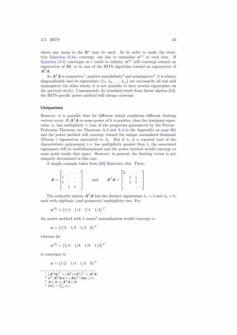
3.3. HITS 43
where any norm in the Rn may be used. So in order to make the itera-
tion Equation (3.3a) converge, one has to normalise x(t) at each step. IfEquation (3.3) converges as t tends to infinity, x(t) will converge toward aneigenvector of M , or in case of the HITS algorithm toward an eigenvector ofATA.
As ATA is symmetric1, positive semidefinite2 and nonnegative3, it is alwaysdiagonalizable and its eigenvalues {λ1, λ2, . . . , λm} are necessarily all real andnonnegative (in other words, it is not possible to have several eigenvalues onthe spectral circle). Consequently, by standard result from linear algebra [24],the HITS specific power method will always converge.
Uniqueness
However, it is possible that for different initial conditions different limitingvectors occur. If ATA or some power of it is positive, then the dominant eigen-value λ1 has multiplicity 1 (one of the properties guaranteed by the Perron–Frobenius Theorem, see Theorems A.2 and A.3 in the Appendix on page 96)and the power method will converge toward the unique normalized dominant(Perron–) eigenvector associated to λ1. But if λ1 is a repeated root of thecharacteristic polynomial, i. e. has multiplicity greater than 1, the associatedeigenspace will be multidimensional and the power method would converge tosome point inside that space. However, in general, the limiting vector is notuniquely determined in this case.
A simple example taken from [20] illustrates this. There,
A =
· · · ·1 · · ·1 · · ·· 1 1 ·
and ATA =
2 · · ·· 1 1 ·· 1 1 ·· · · ·
The authority matrix ATA has two distinct eigenvalues λ1 = 2 and λ2 = 0,each with algebraic (and geometric) multiplicity two. For
x(0) =(
1/4 1/4 1/4 1/4)
T
the power method with 1–norm4 normalization would converge to
x =(
1/3 1/3 1/3 0)
T
whereas for
x(0) =(
1/4 1/8 1/8 1/2)
T
it converges to
x =(
1/2 1/4 1/4 0)
T
1`
ATA´T
= (AT )`
AT´T
= ATA2 xT (ATA)x = (Ax)T (Ax) ≥ 03 A � 0 ⇒ ATA � 04 ‖x‖1 =
P
i |xi|
44 CHAPTER 3. RANKING SCHEMES
An explanation In fact, at the heart of this uniqueness problem is the re-ducibility of ATA. If it is irreducible, then it has a unique (up to a scalarmultiple) dominant Perron eigenvector and the uniqueness problem cannotarise. This follows directly from the Perron–Frobenius Theorem. It ensuresthat if ATA is irreducible it possesses an unique dominant positive eigenvec-tor, and that’s the one the power method will converge to (can easily be seenin Equation (3.4)).
However, in the case of reducibility, obviously ATA is not positive by itselfnor will there be a positive power of it that is strictly positive. So there is nounique dominant eigenvector and convergence depends on the initial condition.
Be aware that irreducibility of A is not sufficient for irreducibility of ATA:A simple example can demonstrate this potential problem. Choosing a cycle oflength n (which obviously is strongly connected, hence irreducible) correspondsto A = Π n, where Π n is a permutation of the identity matrix of order n ≥ 2.It follows ATA = Π
TnΠ n = Π
−1n Π n = idn in this case (as Π n is orthogonal).
The identity matrix being reducible, we have an irreducible adjacency matrixA = Π n resulting in a reducible authority matrix ATA = idn.
PageRank encounters the same uniqueness problem, and a similar trick aswe shall describe for PageRank (cf. Subsection 3.4.2 on page 46) may be appliedhere order to force uniqueness. Another possibility would be not to randomlyinitialize the score vectors, but to always start off with x(0) = y(0) = 1n/n,which guarantees convergence to the same limit. A more elegant way howeveris suggested in [45] using the so–called “exponentiated input to HITS”.
Rate of convergence
The convergence and uniqueness issues above as well as the rate of convergencefollow directly from general results on the power method, see for example [24].The iteration equation Equation (3.3) on page 40 in the case where the domi-nant eigenvalue has multiplicity 1 can be written as follows:
Assume that M := ATA is irreducible. As M is symmetric, it has n mu-tually orthogonal eigenvectors ν1, . . . ,νn (corresponding to the n eigenvaluesλ1, λ2, . . . , λn with |λ1| > |λ2| ≥ |λ3| ≥ . . . ≥ |λn|) which form a basis of Rn.We thus may write the starting vector x(0) as a linear combination
x(0) = c1ν1 + . . . + cnνn
If c1 6= 0 — in other words demanding that the initial vector is not or-thogonal to the dominant eigenvector ν1 — it follows from Equation (3.3) onpage 40 that at iteration step t
x(t) = M tx(0) = c1λt1
ν1 +
n∑
j=2
cj
c1
(
λj
λ1
)t
νj
(3.4)
Here it is clear that the error is of the order of (λ2/λ1)t and hence the rate of
convergence is dictated by the ratio of λ2/λ1 which is particularly importantfor the PageRank algorithm.
If M had been reducible, Equation (3.4) would have more than one termbefore the summation spanning the multidimensional eigenspace into which thepower method would converge to, depending on the initial condition (startingvector).
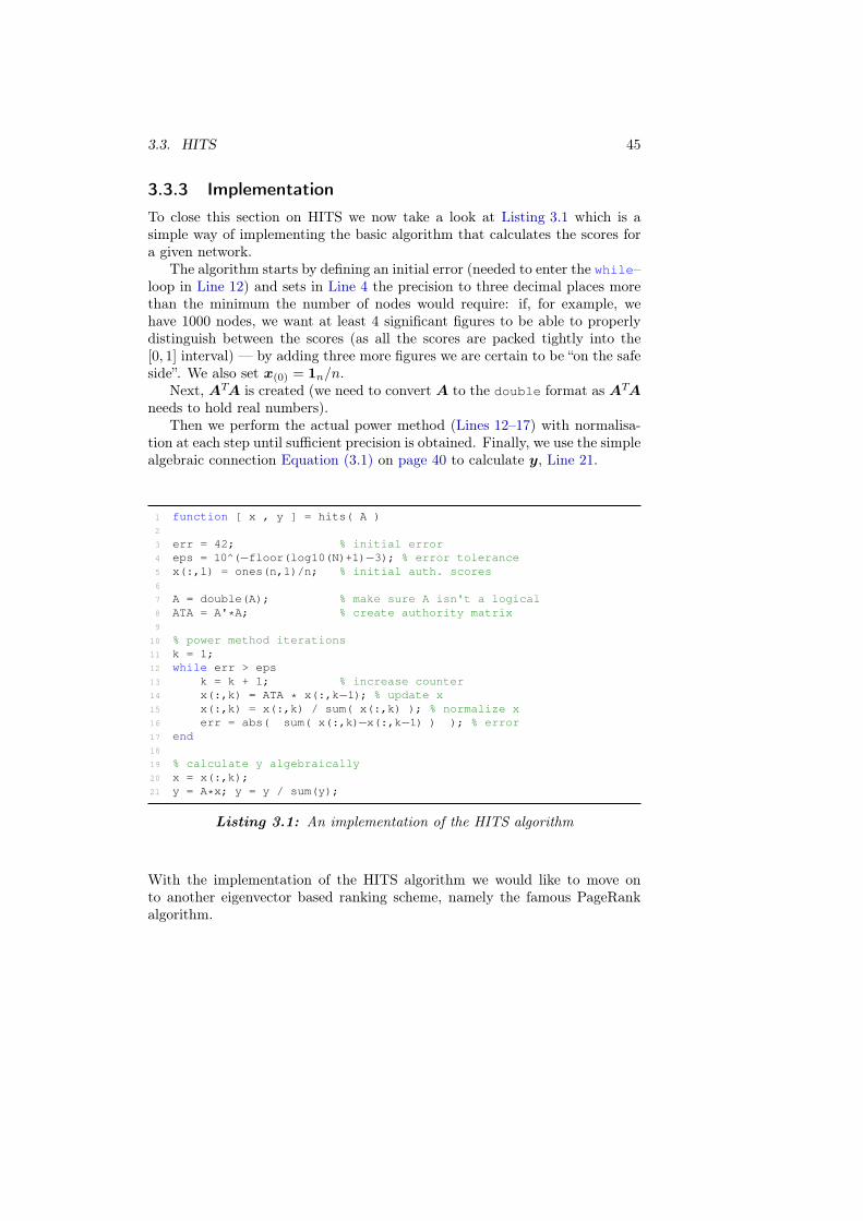
3.3. HITS 45
3.3.3 Implementation
To close this section on HITS we now take a look at Listing 3.1 which is asimple way of implementing the basic algorithm that calculates the scores fora given network.
The algorithm starts by defining an initial error (needed to enter the while–loop in Line 12) and sets in Line 4 the precision to three decimal places morethan the minimum the number of nodes would require: if, for example, wehave 1000 nodes, we want at least 4 significant figures to be able to properlydistinguish between the scores (as all the scores are packed tightly into the[0, 1] interval) — by adding three more figures we are certain to be “on the safeside”. We also set x(0) = 1n/n.
Next, ATA is created (we need to convert A to the double format as ATA
needs to hold real numbers).Then we perform the actual power method (Lines 12–17) with normalisa-
tion at each step until sufficient precision is obtained. Finally, we use the simplealgebraic connection Equation (3.1) on page 40 to calculate y, Line 21.
1 function [ x , y ] = hits( A )
2
3 err = 42; % initial error
4 eps = 10^(−floor(log10(N)+1)−3); % error tolerance
5 x(:,1) = ones(n,1)/n; % initial auth. scores
6
7 A = double(A); % make sure A isn't a logical
8 ATA = A'*A; % create authority matrix
9
10 % power method iterations
11 k = 1;
12 while err > eps
13 k = k + 1; % increase counter
14 x(:,k) = ATA * x(:,k−1); % update x
15 x(:,k) = x(:,k) / sum( x(:,k) ); % normalize x
16 err = abs( sum( x(:,k)−x(:,k−1) ) ); % error
17 end
18
19 % calculate y algebraically
20 x = x(:,k);
21 y = A*x; y = y / sum(y);
Listing 3.1: An implementation of the HITS algorithm
With the implementation of the HITS algorithm we would like to move onto another eigenvector based ranking scheme, namely the famous PageRankalgorithm.
46 CHAPTER 3. RANKING SCHEMES
3.4 PageRank
Since early 1996 Larry Page and Sergey Brin, at the time two Ph.D. candidatesat Stanford University, have been working on a new concept for a search enginefor the world wide web, [13, 52], which was first called “BackRub”, but laterrenamed to “Google”5. In 1998 they founded Google Inc. as all the other majorsearch engine companies were not interested in their new system. The basisof Google was and remains the PageRank algorithm, which, just like HITS,analyzes the hyperlink structure of web to give a ranking for search results.Let’s take a look at the basic concepts and some mathematical background.
3.4.1 Concept
After crawling and indexing the web, PageRank analyzes the link structure todetermine the “global” importance of a page. At query time, all query relateddocuments are retrieved from an inverted index and then ranked according totheir PageRanks, allowing for an almost instantaneous reply to user queries.
The “raw” google matrix
Basic idea The PageRank measure of importance of a page can be seen asweighted votes from all the other pages, weighted by the importance of thelinking (voting) pages themselves and the number of outlinks of those pages:
r(P ) =∑
Q∈BP
r(Q)
|Q| (3.5)
where BP is the set of all pages pointing to page P , r(Q) being the PageRankof page Q and |Q| representing the number of outlinks from page Q. So inorder to have a high PageRank, a page P wants to have as many inlinks aspossible, quality sites pointing at it with at best no other links on these pages.This makes sense, when we consider that if the inlink is only one out of manyit might not be as important as being the sole reference on the linking page.
Iterative approach Because of the recursive definition of PageRank, compu-tation of it necessarily needs iteration. So arbitrarily assign each of the n PagesP1, . . . , Pn an initial ranking, say r(0)(Pi) = 1/n and then successively refinetheir PageRanks by computing
r(t)(Pi) =∑
Q∈BPi
r(t−1)(Q)
|Q| , for t = 1, 2, 3, . . . (3.6)
Combining all the PageRanks in a row vector πT(t) =
(
r(t)(P1) . . . r(t)(Pn))
and creating a normalized hyperlink matrix P with
pij =
{
1/|Pi|, if Pi links to Pj
0, otherwise
5 The word “google” is a common spelling of “googol”, the term coined by Milton Sirotta.In 1938 he was nine years old and a nephew of the American mathematician Edward Kasner,who asked the boy to find a word for the number 10100 . . .
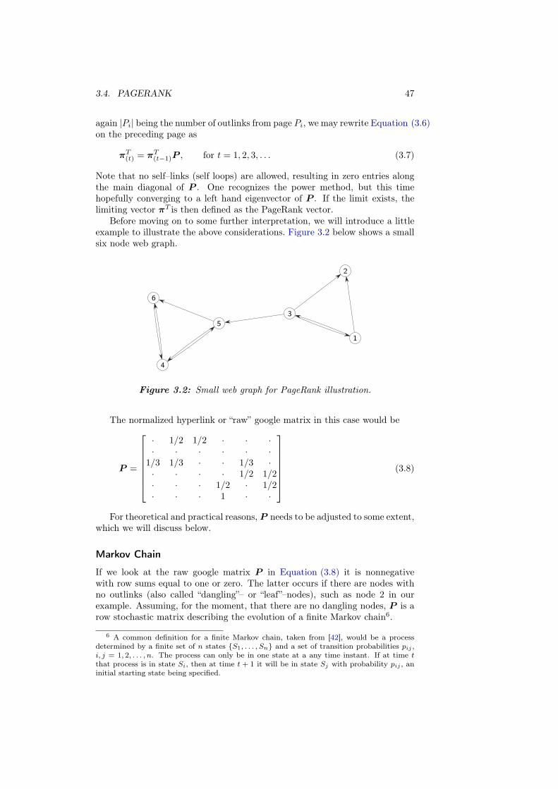
3.4. PAGERANK 47
again |Pi| being the number of outlinks from page Pi, we may rewrite Equation (3.6)on the preceding page as
πT(t) = πT
(t−1)P , for t = 1, 2, 3, . . . (3.7)
Note that no self–links (self loops) are allowed, resulting in zero entries alongthe main diagonal of P . One recognizes the power method, but this timehopefully converging to a left hand eigenvector of P . If the limit exists, thelimiting vector πT is then defined as the PageRank vector.
Before moving on to some further interpretation, we will introduce a littleexample to illustrate the above considerations. Figure 3.2 below shows a smallsix node web graph.
1
2
3
4
5
6
Figure 3.2: Small web graph for PageRank illustration.
The normalized hyperlink or “raw” google matrix in this case would be
P =
· 1/2 1/2 · · ·· · · · · ·
1/3 1/3 · · 1/3 ·· · · · 1/2 1/2· · · 1/2 · 1/2· · · 1 · ·
(3.8)
For theoretical and practical reasons, P needs to be adjusted to some extent,which we will discuss below.
Markov Chain
If we look at the raw google matrix P in Equation (3.8) it is nonnegativewith row sums equal to one or zero. The latter occurs if there are nodes withno outlinks (also called “dangling”– or “leaf”–nodes), such as node 2 in ourexample. Assuming, for the moment, that there are no dangling nodes, P is arow stochastic matrix describing the evolution of a finite Markov chain6.
6 A common definition for a finite Markov chain, taken from [42], would be a processdetermined by a finite set of n states {S1, . . . , Sn} and a set of transition probabilities pij ,i, j = 1, 2, . . . , n. The process can only be in one state at a any time instant. If at time t
that process is in state Si, then at time t + 1 it will be in state Sj with probability pij , aninitial starting state being specified.
48 CHAPTER 3. RANKING SCHEMES
The Markov chain whose evolution P represents (given that there are norows with all zeros) can be interpreted as a random walk on the web: a userinfinitely surfing the world wide web by randomly clicking on one of the linkson each page with equal probability depending on the number of outlinks ofthe current page. The probability of the surfer on page i clicking on the linkleading to page j would correspond to the entry pij .
As for nonnegative matrices, the dominant eigenvalue is bounded by theminimum and maximum row sums [42], the Perron–eigenvalue of a stochasticmatrix is always 1. Consequently, if the PageRank iteration Equation (3.7) onthe previous page converges, it converges to the left–hand eigenvector πT of P
satisfying
πT = πT P with πT1n = 1 (3.9)
This corresponds to the limiting, stationary or steady–state distribution ofthe Markov chain [43]. Intuitively, one could think of it as the long termdistribution of the time spent on the different pages of our eternally surfingworld wide web user.
3.4.2 Computation
As mentioned before, calculating the PageRank comes down to solving the left–hand eigenvector problem Equation (3.9). So if the dangling nodes are takencare of, it seems that all one needs to do is iterate the power method longenough until a satisfying degree of precision is reached. The problem is that, incontrast to HITS, the occurring matrix is not based on a small subset of nodesbut on all the nodes of the world wide web. Google reported in November 2004to have indexed more than 8 billion pages, hence the google matrix would be8–billion–dimensional, [25]. This is the reason why the PageRank calculationhas been called “the worlds largest matrix computation” [48].
This is certainly a challenging topic, but as we won’t deal with matrices ofthis size, we do not need to look at the practical issues in handling such a hugematrix and calculations based on it.
Adjusting P
At this point we should rather direct our attention to how P needs to bemanipulated in order to assure convergence of the power method toward aunique solution.
Taking care of dangling nodes In the above discussion we assumed that P
has no rows with all zeros. An easy remedy for this would be to replace thezeros in these rows by 1/n–entries, where n is, of course, the order of P . Thismodified version P ,is called the transition matrix. An interpretation of thismodification would be that our passionate surfer randomly jumps to anotherpage (for example by manually entering its URL in the location bar), once hearrived at a page where he has no links to click on.7
7 Google however uses a more realistic distribution than the uniform one as it is apparentlynot always equally likely for him to jump to any other page on the web.
3.4. PAGERANK 49
For our small web from Figure 3.2 on page 45 this modification would leadto the following transition matrix
P =
· 1/2 1/2 · · ·1/6 1/6 1/6 1/6 1/6 1/61/3 1/3 · · 1/3 ·· · · · 1/2 1/2· · · 1/2 · 1/2· · · 1 · ·
(3.10)
Fixing reducibility Another problem, that will almost always occur when deal-ing with real web page data, is that P will be reducible. The interpretation ofthat would be that the Markov chain eventually gets trapped at some stage (insome subgraph), which in return usually will depend on the initial conditionschosen. This is the same uniqueness problem we had when dealing with HITS,cf. Subsection 3.3.2 on page 41.
By reordering the states of the chain, the transition matrix P can be madeto have the canonical form Equation (A.1) on page 95. There, once a statein S2 is reached, the chain gets trapped in that set. Usually there are severalconnected components instead of one single big one (the case of connectedness)and the chain can end up in any one of them, depending on the initial conditionchosen.
To fix reducibility and convergence issues, the following convex combinationwas suggested by Brin and Page as passe–partout solution, as it creates astrictly positive matrix:
¯P = αP + (1− α)1n×n
n≻ 0 (3.11)
with 1n×n being the n × n matrix with all ones and α ∈ [0, 1] the so–called“fudge” factor (or more technically the “damping”–factor, as it limits the extentto which a document’s rank can be inherited by the documents it links to).
A possible interpretation for α would be the surfer’s tendency to sometimes“jump” directly to a different page by manually entering its URL into theaddress bar. So (1 − α) can be seen as the probability that our passionateworld wide web user would “teleport” himself to any another page (with equalprobability), ignoring possible links on the current page.
This is a special case of the more general formulation
¯P = αP + (1− α)1nvT (3.12)
where vT is the so–called personalization vector. This vector must be a prob-ability vector and each element can be interpreted as the probability that oursurfer would “teleport” himself to the corresponding page. A non–uniform dis-tribution makes much more sense, as it is not equally as likely to enter anypossible URL.
3.4.3 Iterating
Rate of convergence
Using the matrix given by Equation (3.11) has a very nice side effect. Aspointed out in Subsection 3.3.2 on page 42, the rate of convergence is gov-
50 CHAPTER 3. RANKING SCHEMES
erned by the degree of separation between the dominant and the subdominanteigenvalues. By its nature, the link structure of the world wide web brings|λ2| extremely close to one, [38]. The above convex combination affects theeigendistribution of ¯P in such a way that if S(P ) = {1, λ2, . . . , λn} is the spec-trum of P , then S( ¯P ) = {1, αλ2, . . . , αλn}, cf. [37].8 Thus the asymptotic rateof convergence boils down to how fast αt tends to 0.
Now this leads us to a well discussed “dilemma”. Decreasing α speeds upconvergence, but alters the actual transition matrix which results in movingaway from the true nature of the web. Increasing α on the other hand dra-matically slows down convergence and besides that, sensitivity issues start toappear, as described in Subsection 4.5.2 on page 76. Brin and Page report touse an α around 0.85, [13], which commonly agreed to be a good choice.
Precision
Due to the stochastic nature of πT , all the documents’ PageRanks need to betightly packed into a section of the [0, 1] interval. For n > 8 · 109 an accuracyof at least 10−9 is needed, resulting in a minimum of about 127 iterations withα = 0.85. However, as comparisons at query time will only be made between asmall subset of elements of πT , less accuracy than that is required. Brin andPage report success using only between 50 to 100 iterations.
In our example from Figure 3.2 on page 45, with α = 0.9 one would needat least 23 iterations to reach a precision9 of 10−5, resulting in
πT =(
0.03721 0.05396 0.04151 0.37508 0.20600 0.28624)
and thus a ranking with decreasing PageRank importance of 4, 6, 5, 2, 3, 1.
3.4.4 Implementation
To close this section on PageRank we would like to present a simple imple-mentation of the basic algorithm, which is shown in Listing 3.2 on the facingpage.
It can easily be seen that if we use the ¯P from Equation (3.11) in the powermethod iteration we can rewrite Equation (3.7) on page 45 as
πT(t) = πT
(t−1)¯P
= απT(t−1)P + (1− α)πT
(t−1)
1n×n
n
= απT(t−1)P + (1− α)
1n
n(3.13)
which is the actual iteration equation at the heart of our implementation. Thisway we can split off some work that, effectively, only needs to be carried outonce instead of at every iteration step.
8 In fact, Haveliwala et al. prove in [30] that under given circumstances the second largesteigenvalue of ¯
P actually equals α.9 Precision τ here being the maximum change allowed for any component of πT
(t)between
iteration steps t and t − 1, i. e. τ = maxi |π(t)i− π(t−1)i
|
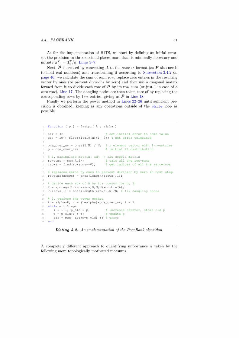
3.4. PAGERANK 51
As for the implementation of HITS, we start by defining an initial error,set the precision to three decimal places more than is minimally necessary andinitiate πT
(0) = 1Tn/n, Lines 3–7.
Next, P is created by converting A to the double format (as P also needsto hold real numbers) and transforming it according to Subsection 3.4.2 onpage 46: we calculate the sum of each row, replace zero entries in the resultingvector by ones (to prevent divisions by zero) and then use a diagonal matrixformed from it to divide each row of P by its row sum (or just 1 in case of azero row), Line 17. The dangling nodes are then taken care of by replacing thecorresponding rows by 1/n–entries, giving us P in Line 18.
Finally we perform the power method in Lines 22–26 until sufficient pre-cision is obtained, keeping as any operations outside of the while–loop aspossible.
1 function [ p ] = fastpr( A , alpha )
2
3 err = 42; % set initial error to some value
4 eps = 10^(−floor(log10(N)+1)−3); % set error tolerance
5
6 one_over_ns = ones(1,N) / N; % n element vector with 1/n−entries7 p = one_over_ns; % initial PR distribution
8
9 % 1. manipulate matrix: adj −> raw google matrix
10 rowsums = sum(A,2); % calc all the row−sums11 zrows = find(rowsums==0); % get indices of all the zero−rows12
13 % replaces zeros by ones to prevent division by zero in next step
14 rowsums(zrows) = ones(length(zrows),1);
15
16 % devide each row of A by its rowsum (or by 1)
17 P = spdiags(1./rowsums,0,N,N)*double(A);
18 P(zrows,:) = ones(length(zrows),N)/N; % fix dangling nodes
19
20 % 2. perform the power method
21 P = alpha*P; z = (1−alpha)*one_over_ns; i = 1;
22 while err > eps
23 i = i+1; p_old = p; % increase counter, store old p
24 p = p_old*P + z; % update p
25 err = max( abs(p−p_old) ); % error
26 end
Listing 3.2: An implementation of the PageRank algorithm.
A completely different approach to quantifying importance is taken by thefollowing more topologically motivated measures.
52 CHAPTER 3. RANKING SCHEMES
3.5 Centrality measures
In the following section, we take a different approach to ranking, an approachthat is not an eigenvector based iterative method like the two we have justfinished discussing.
We will introduce three different notions of centrality used to identify (atleast geometrically) important nodes: excentricity, status and centroid value.These classical measures have been around for many years and extensivelystudied as they are especially useful in resource allocation problems and trans-portation networks.
Using notions of centrality to rank nodes in a network is immediate: themore central a node, the more important it must be. Central nodes are thecrossroads of a network and may give an intuitive idea of the flows of infor-mation. Moreover, in the spirit of graph evolution models, these nodes usuallyreflect some historical importance, as the network must have grown “around”them.
These considerations suggest the use of centrality measures for ranking, andtheir usage in biological networks has been recently proposed in [63]. Each ofthe following three measures will first be motivated by some intuitive exampleof their use, then defined properly and finally implemented.
3.5.1 Excentricity
Motivation and Definition
Suppose you are an urban planner and it is your task to place a fire station. Ofcourse, you want to place it in such a way that the worst case response time isminimal. In a simple traffic network setting, where nodes correspond to placesand edges to the roads connecting them (under the assumption the locations areseparated by unit distances), this typical facility allocation problem searchesthe nodes with minimal maximum distance to all others.
The maximum distance from one node to all other nodes is called excentri-
city:
Definition 3.1 (Excentricity)In a connected graph G = (V, E), the excentricity of a vertex v ∈ V,
denoted e(v), is defined as the maximum over all the distances to the othernodes, i. e. e(v) = maxu∈V lvu.
The radius of the graph, denoted ρ(G ), is defined as the minimal excentri-city of its nodes, i. e. ρ(G ) = minv∈V e(v).
The center of the graph, denoted C(G ), is the set of vertices with excentri-city equal to the graph’s radius, i. e. C(G ) =
{
v ∈ V∣
∣e(v) = ρ(G )}
.
Note that the maximal excentricity over all vertices in a (connected) graphis the graph’s diameter, d(G ) = maxv∈V e(v).
We will now see one use of our somewhat different definition of the dis-tance matrix.10 As we don’t always have the “luxury” of a connected graph,
10 That is that the distance between mutually not reachable nodes is set to n (the totalnumber of nodes), see Subsection 1.3.3 on page 7
3.5. CENTRALITY MEASURES 53
our specialized distance matrix allows for a meaningful extension of the abovedefinition to disconnected graphs. It is clear that the smaller the excentricityof a node, the more central it is. However, a node that is “isolated” in some way(that is at least one other node cannot be reached from it), will be penalizedby the large value n and fall “out of competition” for centrality.
In our example of the “fire station placement problem”, its the center set ofthe traffic network graph that contains all the nodes that solve the problem.It is interesting to note that this set is always contained in a single subgraph,which is a star (that is a connected graph without articulation points11), [29].
Calculation
The calculation of the excentricities of nodes follows directly from its defi-nition and is straightforward once we have got the distance matrix D of thenetwork. The vector e containing the excentricity of each node would then bee = max(D,[],2).
3.5.2 Status
Motivation and Definition
Imagine you are to decide on where to place a new shopping mall. It will bebest for business if most people could reach it as easily as possible, i. e. youdemand minimum average driving time to it.
A classical resource allocation concept to help you out in this case is calledstatus:
Definition 3.2 (Status)In a connected graph G = (V, E), the status of a vertex v ∈ V, denoted
s(v), is defined as the sum over the distances to all the other nodes in the graph,i. e. s(v) =
∑
u∈V luv
The status of the graph, denoted s(G ), is defined as the minimal statusof its nodes, i. e. σ(G ) = minv∈V s(v).
The median of the graph, denoted M(G ), is the set of vertices with statusequal to the graph’s status, i. e. M(G ) =
{
v ∈ V∣
∣s(v) = σ(G )}
.
The definition of status was introduced by Frank Harary in a sociometricalcontext, [28], however the concepts of center and median of a graph were alreadyconsidered by Camille Jordan in 1869, [33]. In the above example, the “shoppingmall placement problem” would be solved by all the nodes in the median set.
Note that instead of the status, one may prefer to consider the averagedistance between one node and all the other nodes. In case of connected graphs,this is equivalent to the status, as the average distance would simply be thestatus divided by e− 1.
As for excentricity, our modified version of the distance matrix allows for asensible extension of the above definition to disconnected graphs.
11 An articulation point (also called cut vertex) of a graph G is a vertex whose removaldisconnects G . Node 1 in Figure 3.3(a) on page 54 is such an articulation point.
54 CHAPTER 3. RANKING SCHEMES
Calculation
Again, calculation is trivial once we have the distance matrix D of the graph.The vector containing all the stati of the nodes would be s = sum(D,2).
3.5.3 Centroid value
Motivation and Definition
Keeping ourselves busy with placing shops, we are, in a different situation,aware of a competitor who also wants to place a shop. Under the assumptionthat customers always buy at the nearest shop, where should we place ourshop, knowing that the competitor will place his shop at some later stage?
The following considerations give us an answer to that question. Let’smodel the problem with a graph where the vertices are the customers and theedges correspond to the road network, each edge representing a unit distance.The customers always buy at the closest store and in case of equal distancesshopping is equally likely at either store.
For vertices u and v let Vuv ={
w ∈ V∣
∣lwu < lwv
}
be the set of all the othervertices that are closer to u than to v. Letting z(u, v) = |Vuv| − |Vvu|, it isclear the we should place our shop in at the location u that maximizes z(u, v)over all possible locations v for our competitor, who will then naturally choosea node v that minimizes z(u, v), so s(v) −→ minv 6=u s(v).
Entringer et al. prove in [18] that s(u) + |Vuv| = s(v) + |Vvu| for all con-nected graphs. With this identity we can write z(u, v) = −s(u) + s(v), an thesolution to the shop placement problem would be to look for vertices u forwhich z(u, v) = −s(u) + minv 6=u s(v) is maximal.
This motivates the definition of the centroid value:
Definition 3.3 (Centroid value)In a connected graph G = (V, E), the centroid value of a vertex v ∈ V,
denoted z(v), is defined as z(v) = s(v)−minu6=vs(u).
The centroid value of the graph, denoted χ(G ), is defined as the minimalcentroid value of its nodes, i. e. ζ(G ) = minv∈V z(v).
The centroid of the graph, denoted C(G ), is the set of vertices with centroidvalue equal to the graph’s centroid value, i. e. C(G ) =
{
v ∈ V∣
∣c(v) = ζ(G )}
.
Note that this definition is different from the one Peter J. Slater gave in[57], namely in that the sign of z(u, v) has been inverted. The reason for thatis purely aesthetic and was suggested in [63]: in analogy to excentricity andstatus we would like this third centrality measure to be minimal at the mostcentral nodes. In fact, contrary to the other measures, the centroid value of anode might very well become zero, or even negative.
If in a connected graph G = (V, E) we find a node v with centroid valuez(v) = 0, it implies that s(v) = minu6=v s(u) = σ(G ). Hence, by definition,v ∈ M(G ) and there exists at least one other node with the same minimalstatus, i. e. |M(G )| ≥ 2.
However we can find z(v) < 0 only for at most one node v. In this case,s(v) is the unique minimum of all the stati, and M(G ) = C(G ) =
{
v}
.

3.6. DAMAGE 55
Calculation
Due to the fact that for each node we need to determine the minimum of thestatus over all other nodes we cannot calculate the vector containing all thecentroid values with a single command; we have to use a for–loop. First wecalculate all the stati and store them in s. Then, in the loop, we remove ateach step the current node from s and finally search for the minimum, seeListing 3.3 below.
1 function z = centroid( D )
2
3 z = zeros(n,1); % initialize
4 s = sum(D,2); % calculate all the stati
5 for i = 1:n
6 tempstat = s; % temporarily store s
7 tempstat(i) = []; % remove current
8 z(i) = s(i) − min(tempstat);
9 end
Listing 3.3: Function returning the centroid values of all the nodes in a graph.
Yet another, radically different approach to measuring importance is taken byour last ranking scheme, namely the one induced by “damage”.
3.6 Damage
We would like to close this chapter by introducing a seventh measure: dam-
age. This measure has been introduced in [39] for bipartite graphs, and morerecently for undirected graphs in [56].
3.6.1 Motivation and Definition
In biological networks for example, another idea of the importance of a node(enzyme) would be the effect its removal would have. One missing enzymecould prevent the production of a number of proteins and thus have a criticaleffect on the entire organism.
The damage value of a node has been introduced to quantify the effect ofthe deletion of that particular node. Similar to [56] we define the damage valueof a node as follows:
Definition 3.4 (Damage)In a graph G = (V, E), let Gv = (Vv, Ev) be the connected component that
contains node v, so v ∈ Vv, and let Gv = (Vv, Ev) be the largest connectedcomponent of Gv after the removal of node v, so v /∈ Vv.
Then the value
ð(v) = |Vv| − |Vv|
is the damage value (or just damage) of node v.
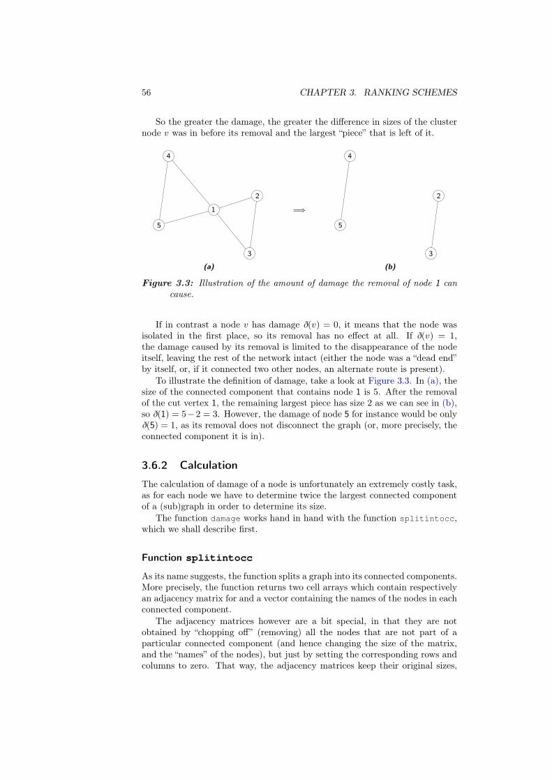
56 CHAPTER 3. RANKING SCHEMES
So the greater the damage, the greater the difference in sizes of the clusternode v was in before its removal and the largest “piece” that is left of it.
1
2
3
4
5
(a)
=⇒
2
3
4
5
(b)
Figure 3.3: Illustration of the amount of damage the removal of node 1 cancause.
If in contrast a node v has damage ð(v) = 0, it means that the node wasisolated in the first place, so its removal has no effect at all. If ð(v) = 1,the damage caused by its removal is limited to the disappearance of the nodeitself, leaving the rest of the network intact (either the node was a “dead end”by itself, or, if it connected two other nodes, an alternate route is present).
To illustrate the definition of damage, take a look at Figure 3.3. In (a), thesize of the connected component that contains node 1 is 5. After the removalof the cut vertex 1, the remaining largest piece has size 2 as we can see in (b),so ð(1) = 5−2 = 3. However, the damage of node 5 for instance would be onlyð(5) = 1, as its removal does not disconnect the graph (or, more precisely, theconnected component it is in).
3.6.2 Calculation
The calculation of damage of a node is unfortunately an extremely costly task,as for each node we have to determine twice the largest connected componentof a (sub)graph in order to determine its size.
The function damage works hand in hand with the function splitintocc,which we shall describe first.
Function splitintocc
As its name suggests, the function splits a graph into its connected components.More precisely, the function returns two cell arrays which contain respectivelyan adjacency matrix for and a vector containing the names of the nodes in eachconnected component.
The adjacency matrices however are a bit special, in that they are notobtained by “chopping off” (removing) all the nodes that are not part of aparticular connected component (and hence changing the size of the matrix,and the “names” of the nodes), but just by setting the corresponding rows andcolumns to zero. That way, the adjacency matrices keep their original sizes,

3.6. DAMAGE 57
1 function [ ccsA , ccsN ] = splitintocc( A )
2
3 % calculate matrix Asum2. nonzero entries correspond to mutually
4 % reachable nodes (see function avl for more details).
5 n = length(A); nn = n^2; m = 0; ∆nnz = 42;
6 Asum2 = logical(speye(n)); Am = Asum2;
7 warning('off','MATLAB:conversionToLogical'); % we know that issue.
8
9 while (nnz(Asum2) 6= nn) && (∆nnz 6= 0) && (m ≤ n)
10 m = m + 1; Am = logical(double(Am)*A); % new power of A
11 Asum1 = Asum2; Asum2 = Asum1 | Am; % add it to Asum2
12 ∆nnz = nnz(Asum2)−nnz(Asum1); % increase of new paths
13 end
14
15 ncc = 0; ccsA = {}; ccsN = {}; oneton = 1:n; rmved = [];
16
17 % now go through the connected components
18 while ¬isempty(Asum2)19 ncc = ncc + 1;
20
21 % grab all the nodes that are reachable from first node ...
22 thiscc = find(Asum2(1,:));
23
24 % take care of node name changes resulting from the removals ...
25 origind = oneton; origind(rmved) = []; % "simluate" removal
26 thiscc_origind = origind(thiscc);
27 removeme_origind=oneton; removeme_origind(thiscc_origind)=[];
28
29 % now create the different adjacency matrices of the different ccs
30 ccsA{ncc} = A; % take A ...
31 ccsA{ncc}(removeme_origind,:) = false; % set non−cc−members to 0
32 ccsA{ncc}(:,removeme_origind) = false; % ...
33 ccsN{ncc} = thiscc_origind; % and store their names
34
35 % finally get them out of the way
36 Asum2(thiscc,:) = []; Asum2(:,thiscc) = [];
37 rmved = [rmved,thiscc_origind];
38 end
Listing 3.4: Function returning the connected components (and the respectivenodes in these) of a graph.
the nodes keep their “names” and only the nodes that are part of the currentconnected component keep edges attached to them.12
Much of the functionality is similar to our avl function, see Subsection 1.4.2on page 12. Basically, we create a matrix Asum2 which contains a nonzeroelement (i, j) if node i can be reached from node j, which is then used todetermine the connected components.
However, special care needs to be taken in the process: as (in order to savework) we remove nodes along the way, we must keep track of the original namesof the nodes.
12 This has a practical reason, because now slcc(ccsA{x}) will automatically report thecorrect size of the connected component of the nodes in cssN{x}
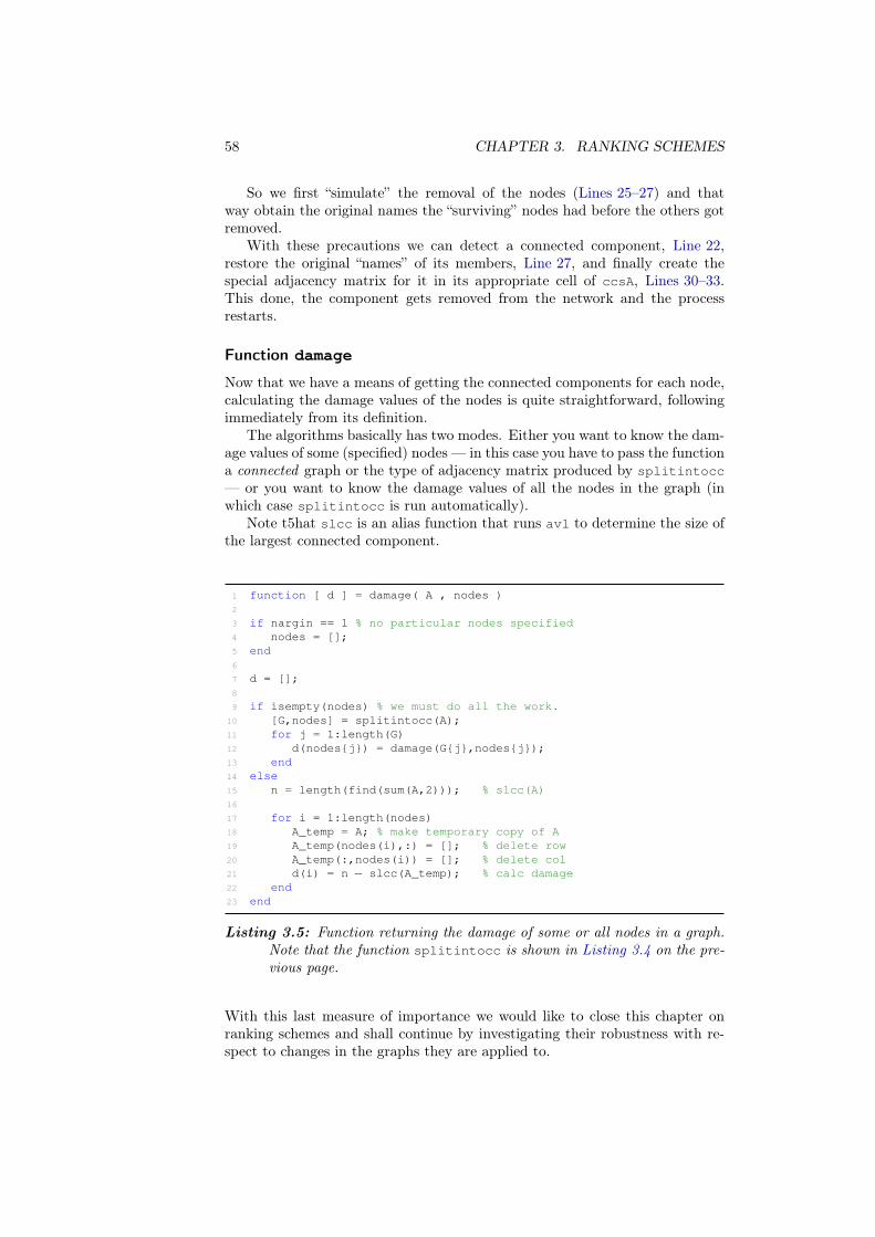
58 CHAPTER 3. RANKING SCHEMES
So we first “simulate” the removal of the nodes (Lines 25–27) and thatway obtain the original names the “surviving” nodes had before the others gotremoved.
With these precautions we can detect a connected component, Line 22,restore the original “names” of its members, Line 27, and finally create thespecial adjacency matrix for it in its appropriate cell of ccsA, Lines 30–33.This done, the component gets removed from the network and the processrestarts.
Function damage
Now that we have a means of getting the connected components for each node,calculating the damage values of the nodes is quite straightforward, followingimmediately from its definition.
The algorithms basically has two modes. Either you want to know the dam-age values of some (specified) nodes — in this case you have to pass the functiona connected graph or the type of adjacency matrix produced by splitintocc
— or you want to know the damage values of all the nodes in the graph (inwhich case splitintocc is run automatically).
Note t5hat slcc is an alias function that runs avl to determine the size ofthe largest connected component.
1 function [ d ] = damage( A , nodes )
2
3 if nargin == 1 % no particular nodes specified
4 nodes = [];
5 end
6
7 d = [];
8
9 if isempty(nodes) % we must do all the work.
10 [G,nodes] = splitintocc(A);
11 for j = 1:length(G)
12 d(nodes{j}) = damage(G{j},nodes{j});
13 end
14 else
15 n = length(find(sum(A,2))); % slcc(A)
16
17 for i = 1:length(nodes)
18 A_temp = A; % make temporary copy of A
19 A_temp(nodes(i),:) = []; % delete row
20 A_temp(:,nodes(i)) = []; % delete col
21 d(i) = n − slcc(A_temp); % calc damage
22 end
23 end
Listing 3.5: Function returning the damage of some or all nodes in a graph.Note that the function splitintocc is shown in Listing 3.4 on the pre-vious page.
With this last measure of importance we would like to close this chapter onranking schemes and shall continue by investigating their robustness with re-spect to changes in the graphs they are applied to.
C H A P T E R 4
Robustness
We devise 4 types of network perturbations and 6
different ways of measuring deviations in rankings,
then present quantitative results as well as some
theoretical results on the ranking’s robustness.
4.1 Introduction
Now that we have discussed different measures suitable for ranking nodes ina network, we should investigate the robustness of the resulting rankings inparticular with respect to variations in the network.
The data gathered in real life is often based on some physical measure-ments. This implies that the data might be inaccurate, incomplete or incorrectto some degree, reasons for that possibly being insufficient precision in thephysical measurements, the influence of noise, or deliberate sampling (giventhat measuring 100% of the system may require unjustifiabilly more time ormoney).
In any case, it is important to know how sensitive the rankings are tovarious types of perturbation. A ranking scheme that inverts the order ofthe nodes when only a few edges are changed will be of little practical use.To analyse the impact of perturbations, we introduce a number of ways tomeasure the deviations between two rankings. We then perturb the networkby incrementally removing, adding or rewiring edges, or removing nodes — asthese are phenomena close to real life problems — and compare the deviationbetween the rankings of the original and the perturbed networks.
For the simulations we used randomly generated Barabási–Albert graphsas their degree distribution resembles those of protein–protein interaction net-works that we are going to look at in the last chapter. Our extensive quan-titative results are also accompanied by a few theoretical results concerningPageRank and HITS.
4.2 Perturbations
As mentioned above, having data which is 100% correct is a rather “utopian”case. Being able to identify important nodes by some ranking is one thing,having a ranking that is also robust to missing or slightly wrong data is another.
Note that perturbing edges has in two ways a rather limited effect, comparedto changing nodes. On the one hand, changing one edge only affects two nodes
59
60 CHAPTER 4. ROBUSTNESS
(but may disconnect the graph) and there are usually much more edges thannodes. On the other hand, removing a node also implies the removal of alledges joining it, so the impact will usually be much greater.
We shall now describe various types of possible perturbations.
4.2.1 Edge perturbations
Edge removal
One of the most intuitive perturbations is surely edge removal. By that, wemean the random deletion of a number of edges.
This would correspond to the case for example, where measurements missedout on some interactions between proteins.
Edge addition
The dual case to edge removal would be edge addition in random positions,similar to the procedure used to generate Erdös–Rényi graphs.
Such a perturbation could be introduced for example by measurement noiseor wrong interpretation of certain results.
Edge rewiring
In the case of edge rewiring, the number of edges stays constant (this timesimilar to the generating algorithm of the Watts–Strogatz model).
This type of perturbation can also be induced by noise or misinterpretationsof lab results.
4.2.2 Node perturbations
Node removal
Another intuitive perturbation would be (random) node removal, i. e. we ran-domly choose a number of nodes and remove them (as well as all the edgesjoining it).
This would correspond to missing out on some (maybe intermediate) reac-tant or additional “ingredient” in some reaction due to either inaccurate mea-surements or deliberate sampling of data.
Node attack
By node attack we mean the systematic and targeted removal of the mostimportant nodes. This is a rather artificial alteration, as it implies some inten-tional act (and the a priori knowledge of the importance of all the nodes). Wetherefore only mention it here, but will not examine it further in this presentwork.

4.3. MEASURES OF DEVIATION 61
Node addition
Node addition would be the random addition of nodes, which must also beaccompanied by the addition of a number of edges connecting those new nodesto the network. As in the biological networks we shall consider later the numberof nodes (proteins) is usually well known (through, for example, sequencing thegenome), it is very unlikely that some perturbation would actually add nodes tothe network. This is the main reason why we shall also leave this perturbationout of the following investigations.
4.3 Measures of deviation
We shall now present six different approaches to measuring the deviations be-tween the ranking of an original and a perturbed network. We will call these“Method 1 – 6”. At the beginning of each we try to give a short and condensedquestion to motivating it.
All methods have in common that they look at the top 5% (plus ties) ofthe nodes in the rankings. We do this mainly for two reasons:
(i) In practice, one is only interested in a few top ranked nodes, not the entireranking (just like a person searching some information on the internetonly checks the first few results a search engine has come up with, so itis most important to know the sensitivity of these results).
(ii) In case of node removal, the total number of nodes and hence “contribu-tions” to the deviation measure decreases. For a meaningful comparison,however, we need a constant number. So, for instance, if we only use asmall (constant) number of top ranked nodes (say a number correspond-ing to 5% of the origininal network size), we can then remove up to 95%of the nodes and still be comparing the same number of deviations.
The first three measures focus on the actual ranks of the nodes. The result-ing deviation measure is calculated by taking the L1–norm of the respectivedeviations in ranking of the nodes, i. e. we sum up the absolute values of thedifferences in places. Conversely, the last three measures are based purely onthe fact whether a node is in the top 5% of the rankings or not.
4.3.1 Using the ranking of the nodes
The following three methods use the ranks1 of nodes to measure the deviation.
Method 1
“How strong an impact has the perturbation on the identificationof highly ranked nodes in the ‘real’ network?”
To answer that question, we compare the ranks of a number of initially topranked nodes (i. e. in the ranking of the unperturbed network) with where they“ended up” after the perturbation.
1 Please note the way we set up our ranking, which is described at the beginningof Subsection 4.3.4 on page 63.

62 CHAPTER 4. ROBUSTNESS
Table 4.1(a) on the current page illustrates this process. Here we have anetwork with 10 nodes and look at the top 50% of the nodes. The measure ofdeviation δ1 would be calculated as follows:
δ1 = |1− 6|︸ ︷︷ ︸
Node 3
+ |1− 2|︸ ︷︷ ︸
Node 8
+ |3− 9|︸ ︷︷ ︸
Node 4
+ |4− 4|︸ ︷︷ ︸
Node 10
+ |4− 1|︸ ︷︷ ︸
Node 1
= 15
Original Perturbed
Rank Node Rank Node
1. 3 1
1. 8 8
3. 4 ·4. 10 10
4. 1 ·6. · 3
7. · ·8. · ·9. · 4
10. · ·(a) Method 1.
1.2.3.4.5.6.7.8.9.10.
Original Perturbed
Rank Node Rank Node
1. 7 9
2. · 7
2. 4 1
4. 1 4
5. 9 2
6. · ·7. · ·7. · ·7. · ·10. 2 ·
(b) Method 2.
1.2.3.4.5.6.7.8.9.10.
Original Perturbed
Rank Node Rank Node
1. 6 5
2. 2 ·3. 10 ·4. · 3
5. · ·5. · 6
7. · ·8. · 2
9. 3 10
10. 5 ·(c) Method 3.
1.2.3.4.5.6.7.8.9.10.
(d) Methods 4, 5 and 6.
L
IO
IP
IO ∩ L
IO ∩ IP
Table 4.1: Illustrations for the five methods used to calculate deviations. Thedots are placeholders for values that are not used / unimportant.
4.3. MEASURES OF DEVIATION 63
Method 2
“How important really are nodes of high rank in the perturbednetwork?”
This question can be answered by looking at the positions of a numberof top ranked nodes from the perturbed graph and compare these with theiroriginal (“real”) ranks.
In Table 4.1(b) on the facing page we illustrate these comparisons for afraction of 50% of the top ranked nodes in the perturbed network. The resultingmethod of deviation δ2 is then calculated with:
δ2 = |1− 5|︸ ︷︷ ︸
Node 9
+ |2− 1|︸ ︷︷ ︸
Node 7
+ |3− 4|︸ ︷︷ ︸
Node 1
+ |4− 2|︸ ︷︷ ︸
Node 4
+ |5− 10|︸ ︷︷ ︸
Node 2
= 13
Method 3
“How big are the maximum deviations between the rankings?”
To quantify this, we first determine all the deviations and then sum up afraction of the biggest deviations.
Looking at a fraction of 50% of the deviations, the dashed gray arrows inTable 4.1(c) on the preceding page correspond to those that are not taken intoaccount as they are smaller then the deviations marked by the solid arrows.We determine δ3 in this case with:
δ3 = |1− 6|︸ ︷︷ ︸
Node 6
+ |2− 8|︸ ︷︷ ︸
Node 2
+ |3− 9|︸ ︷︷ ︸
Node 10
+ |9− 4|︸ ︷︷ ︸
Node 3
+ |10− 1|︸ ︷︷ ︸
Node 5
= 31
4.3.2 Using the number of correctly identified nodes
Method 4
“What’s the chance that a seemingly important node is, in fact,not important?”
To answer this question, we first define two sets: IO is made up of the top5% plus ties of the (original) ranking and IP of the top 5% plus ties of theranking of the perturbed network.2
Then we look at the cardinalities of the sets and their intersection. Thenodes that are identified as important and that really are important would befound in the set IO ∩ IP . If we compare the number of nodes in this set withthe total number of “important” nodes in the perturbed network (IP ), we getan idea of the quality of the ranking.
To set up a deviation measure, now let
δ4 = 1− |IO ∩ IP ||IP |
2 See Table 4.1(d) on the facing page for an illustration of the sets. The numbers 5%and 5% here are chosen arbitrarily to some extent, and they do not necessarly have to beidentical.

64 CHAPTER 4. ROBUSTNESS
This measure can then be interpreted as the probability that a seemingly im-portant node in the perturbed network is, in fact, not really important.
Of course, this measure strongly depends on the chosen “limits” for impor-tance. In the following, we will stick to the suggested top 5% from both theoriginal and the perturbed ranking.
To give a little example, say we take the ranking from Table 4.1(a) onpage 60. Considering 40% and 20% of the top ranked nodes as “important”,we would have IO =
{
3, 8, 4, 10, 1}
(note that even though 40% correspond to4 nodes, we also took node 1 in as place 4. is a tie) and IP =
{
1, 8}
. HenceIO∩IP =
{
1, 8}
and finally δ4 = 1−2/2 = 0 indicating a flawless performanceof the “ranking scheme” behind the two presented rankings.
Method 5
“What’s the probability that an important node does not get iden-tified as such?”
In other words, we now would like to have an idea of how many of the nodesthat really are important do not stay in a certain top fraction of the rankingafter perturbation.
An attempt to answer this question is quite similar to our previous measure.We define the sets IO and IP in the same way as above (i. e. for example top5% plus ties) and then let
δ5 = 1− |IO ∩ IP ||IO|
So the only difference is that we divide by the number of elements in IO insteadof in IP .
4.3.3 Method 6
“What’s the chance that the importance of top ranked nodes getstotally misjudged?”
An example for such a misjudgment would be if originally important nodesend up at the bottom of the ranking of the perturbed graph. So an approachto the question above would be to define an other set, IL, which contains the,say, bottom 25% of the nodes in the ranking of the perturbed graph. We canthen introduce
δ6 =|IO ∩ IL||IO|
That way, δ6 corresponds to the probability that an originally important nodeends up in the bottom quartile of the network.
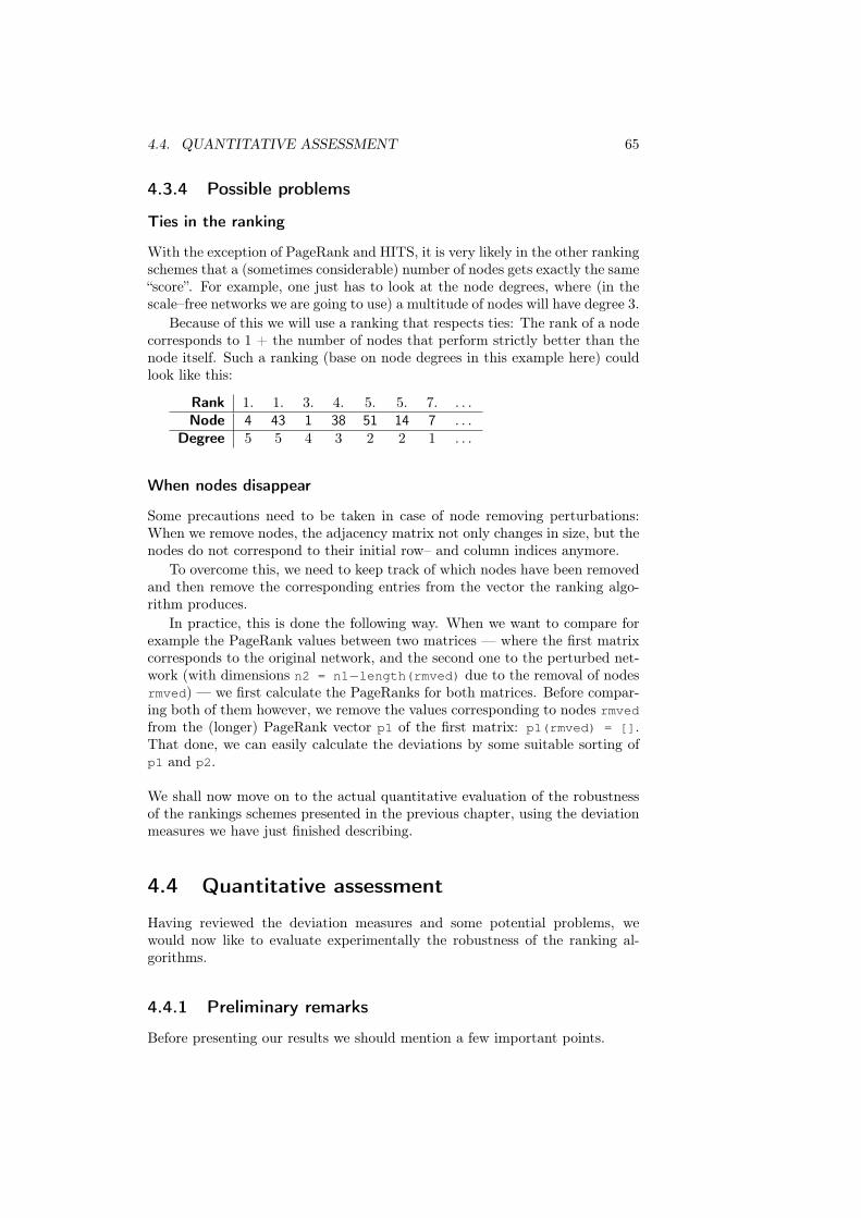
4.4. QUANTITATIVE ASSESSMENT 65
4.3.4 Possible problems
Ties in the ranking
With the exception of PageRank and HITS, it is very likely in the other rankingschemes that a (sometimes considerable) number of nodes gets exactly the same“score”. For example, one just has to look at the node degrees, where (in thescale–free networks we are going to use) a multitude of nodes will have degree 3.
Because of this we will use a ranking that respects ties: The rank of a nodecorresponds to 1 + the number of nodes that perform strictly better than thenode itself. Such a ranking (base on node degrees in this example here) couldlook like this:
Rank 1. 1. 3. 4. 5. 5. 7. . . .Node 4 43 1 38 51 14 7 . . .
Degree 5 5 4 3 2 2 1 . . .
When nodes disappear
Some precautions need to be taken in case of node removing perturbations:When we remove nodes, the adjacency matrix not only changes in size, but thenodes do not correspond to their initial row– and column indices anymore.
To overcome this, we need to keep track of which nodes have been removedand then remove the corresponding entries from the vector the ranking algo-rithm produces.
In practice, this is done the following way. When we want to compare forexample the PageRank values between two matrices — where the first matrixcorresponds to the original network, and the second one to the perturbed net-work (with dimensions n2 = n1−length(rmved) due to the removal of nodesrmved) — we first calculate the PageRanks for both matrices. Before compar-ing both of them however, we remove the values corresponding to nodes rmvedfrom the (longer) PageRank vector p1 of the first matrix: p1(rmved) = [].That done, we can easily calculate the deviations by some suitable sorting ofp1 and p2.
We shall now move on to the actual quantitative evaluation of the robustnessof the rankings schemes presented in the previous chapter, using the deviationmeasures we have just finished describing.
4.4 Quantitative assessment
Having reviewed the deviation measures and some potential problems, wewould now like to evaluate experimentally the robustness of the ranking al-gorithms.
4.4.1 Preliminary remarks
Before presenting our results we should mention a few important points.
66 CHAPTER 4. ROBUSTNESS
Our setup
Due to the number of combinations that result from the different deviation mea-sures (6), different perturbations (4), different ranking schemes (7), differentgraph models (3) and different network parameter combinations (countless),we cannot present all of our results.
The first step in reducing this overwhelming number of possible combina-tions is that we limit ourselves to only looking at a one type of graph and the(fixed) sets of generating parameters: In all of the following, we used scale–freegraphs on n = 3000 nodes and roughly e ≃ 9000 edges — generated with theBarabási–Albert model using n0 = m = 3.
We chose this model not only for reasons of simplicity and the fact that it iswell studied, but mostly because many networks encountered in biology showscale–free characteristics (see Subsection 2.5.2). The actual parameter choiceis of course arbitrary to some extent, but produces graphs similar in size to thereal world graphs we will be looking at in the next chapter.
For each deviation method we will then show the impact of the differ-ent perturbations by comparing the sensitivity of each of the seven rankingschemes. Any of the following values and plots represent the average from 250independent runs of the respective simulation.
The results are plotted using the following markers:
× Node degrees� HITS� PageRank
△ Excentricity♦ Status• Centroid value
For the PageRank rankings we used the standard α = 0.85.
Disconnection
The scale–free graphs we are generating are always connected (this is guaran-teed by the Barabási–Albert model we will use). However, when we start toremove or rewire edges, sooner or later the graph will get disconnected.3
As the disconnection of the graph will significantly influence the centralitybased ranking algorithms it is important to study the point at which the graphsusually become disconnected. We did so by generating 250 scale–free graphsand perturbed them in a similar increasing way (in the exact same way as usedfor the comparisons below). We then took note after how much perturbationthe graph became disconnected.
Figure 4.1 on the next page shows the distributions from these simulations.There, we can see in (a) that the amount of perturbation required for discon-necting the graphs can be as little as 100 or as high as 1600 removed edges.From the 250 graphs generated, the calculated mean was around 785 removededges (with standard deviation of ≈ 266) needed to disconnect the graph.
A similar result holds for edge rewiring, see (b). Disconnection can occurin a broad interval ranging from 100 to 1900 rewired edges which contains thecalculated mean value of ≈ 900 (with standard deviation ≈ 345).
3 This is immediate to see for edge removals; in the rewiring case we could argue that thegraph is turning more and more into an Erdös–Rényi graph. For these graphs, 9000 edges for3000 nodes are far from enough to “guarantee” connectedness, see Theorem 2.1 on page 22.
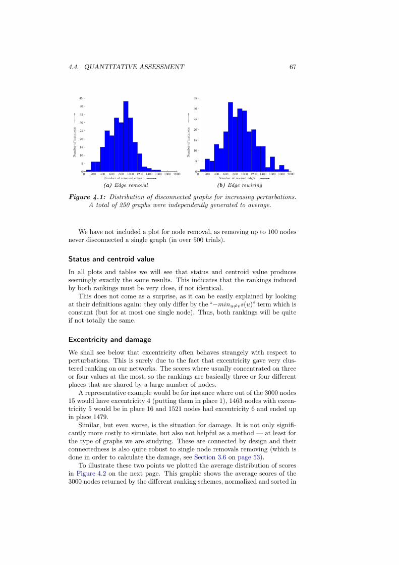
4.4. QUANTITATIVE ASSESSMENT 67N
umber
ofin
stan
ces
GGGGGGA
Number of removed edges GGGGGGA
0 200 400 600 800 1000 1200 1400 1600 1800 20000
5
10
15
20
25
30
35
40
45
(a) Edge removalN
umber
ofin
stan
ces
GGGGGGA
Number of rewired edges GGGGGGA
0 200 400 600 800 1000 1200 1400 1600 1800 20000
5
10
15
20
25
30
35
(b) Edge rewiring
Figure 4.1: Distribution of disconnected graphs for increasing perturbations.A total of 250 graphs were independently generated to average.
We have not included a plot for node removal, as removing up to 100 nodesnever disconnected a single graph (in over 500 trials).
Status and centroid value
In all plots and tables we will see that status and centroid value producesseemingly exactly the same results. This indicates that the rankings inducedby both rankings must be very close, if not identical.
This does not come as a surprise, as it can be easily explained by lookingat their definitions again: they only differ by the “−minu6=vs(u)” term which isconstant (but for at most one single node). Thus, both rankings will be quiteif not totally the same.
Excentricity and damage
We shall see below that excentricity often behaves strangely with respect toperturbations. This is surely due to the fact that excentricity gave very clus-tered ranking on our networks. The scores where usually concentrated on threeor four values at the most, so the rankings are basically three or four differentplaces that are shared by a large number of nodes.
A representative example would be for instance where out of the 3000 nodes15 would have excentricity 4 (putting them in place 1), 1463 nodes with excen-tricity 5 would be in place 16 and 1521 nodes had excentricity 6 and ended upin place 1479.
Similar, but even worse, is the situation for damage. It is not only signifi-cantly more costly to simulate, but also not helpful as a method — at least forthe type of graphs we are studying. These are connected by design and theirconnectedness is also quite robust to single node removals removing (which isdone in order to calculate the damage, see Section 3.6 on page 53).
To illustrate these two points we plotted the average distribution of scoresin Figure 4.2 on the next page. This graphic shows the average scores of the3000 nodes returned by the different ranking schemes, normalized and sorted in

68 CHAPTER 4. ROBUSTNESS
increasing order. We can see that for most of the nodes, the excentricity curveis absolutely flat, meaning that many nodes get the same score. The situationis even more dramatic for the damage scores, see Figure B.2 on page 99, whereeach and every node has the same score.
Node number GGGGGGA
Scor
eGGGGGGA
0 200 400 600 800 1000 1200 1400 1600 1800 2000 2200 2400 2600 2800 30000
0.1
0.2
0.3
0.4
0.5
0.6
0.7
0.8
0.9
1
Figure 4.2: Average distribution of the scores of the different ranking schemeson 200 Barabási–Albert graphs with n = 3000 nodes and n0 = m = 3 .
With these considerations in mind we still kept excentricity and damage inour simulations4, solely for reasons of completeness. We shall present andanalyse the results from these simulations.
4.4.2 Results
Method 1
General remarks Figure 4.3 on the facing page shows the relevant plots forthis first measure. Note that we cannot present results for node removal pertur-bations as some of the originally most highly ranked nodes might get removedwith increasing perturbation. In that case we cannot perform the necessarycomparisons.
4 The results for damage, however, have only been calculated for smaller graphs of 150nodes; these results are shown in the Appendix B on page 97

4.4. QUANTITATIVE ASSESSMENT 69
Number of removed edges GGGGGGA
Dev
iati
onGGGGGGA
0 200 400 600 800 1000 1200 1400 1600 1800 20000
0.2
0.4
0.6
0.8
1
1.2
1.4
1.6
1.8
2
(a) Edge removal
Number of added edges GGGGGGA
Dev
iati
onGGGGGGA
0 200 400 600 800 1000 1200 1400 1600 1800 20000
0.5
1
1.5
2
2.5
3
3.5
4 ×10³
(b) Edge addition
Number of rewired edges GGGGGGA
Dev
iati
onGGGGGGA
0 200 400 600 800 1000 1200 1400 1600 1800 20000
0.2
0.4
0.6
0.8
1
1.2
1.4
1.6
1.8
2 ×10⁴
(c) Edge rewiring
Figure 4.3: Sensitivity for deviation measure 1.
Besides some (explainable) nonlinear behavior for excentricity the othercurves seem quite linear. But in the case of edge addition, PageRank and nodedegrees clearly perform best compared to the other measures.
Edge removal One of the most remarkable things in Figure 4.3(a) is probablythe shape of the curve for the excentricity (△). The error seems to increasefirst but then decreases again after about 600 links have been removed. Thisbehavior however does not reflect the real sensitivity of the rankings, as it canbe explained in the following way.
In the early stages, as edges get removed, the perturbation increases andinitially top ranked nodes might “climb down” the ranking. Obviously, the moreedges get removed, the more likely it is that the graph becomes disconnected.As mentioned in Subsection 4.4.1 on page 64 the majority of the graphs usuallybecame disconnected after about 600 removed nodes.
Now, what happens the moment time the graph becomes disconnect? Onething is, that the distance matrix gets its first set of “penalty entries” with thehigh value n = 3000. As a matter of fact, from that moment on, each row andeach column in the distance matrix must have at least one penalty entry. Asmentioned above, the excentricity of a node corresponds to the maximum entry
70 CHAPTER 4. ROBUSTNESS
in the distance matrix along its corresponding row. Hence suddenly all nodesget the same excentricity, get ranked (shared) first place and the deviation fallsdown to a low, constant value.
The shape of the curve is then produced by the superimposition of the100 series of deviation values that are used to average out the results. Eachgraph in it becomes disconnected at a different point, similar to the shape ofFigure 4.1(a) on page 65.
Edge addition We can see in Figure 4.3(b) that the excentricity performsmuch worse than all the other ranking schemes, which are all roughly equallyas good.
However, the absolute deviations are much smaller (by more than one orderof magnitude) compared to the other perturbations. This might be due to thefact that the graph cannot become disconnected here.
Edge rewiring When it comes to rewiring, we can see in Figure 4.3(c) thatPageRank and node degrees seem to be the best choice as their rankings seemto be much more stable than the other ones. The order of magnitude of thedeviations is surprisingly almost precisely the same as for edge removal.
Also, the same shape for the excentricity curve is manifest. The graphsare becoming disconnected, as they gradually turn into Erdös–Rényi randomgraphs with 3000 nodes and 9000 edges, which will typically not be connected(in average). We thus have the same disconnection issue as for edge removaland a similar explanation for the shape of the curve applies.
Method 2
General remarks The relevant plots for this first measure are shown in Figure 4.4on the next page. There, we can see that most values, again, increase quitelinearly, with the exception of excentricity.
Also, PageRank and node degrees do the best job for each type of pertur-bation, most clearly in case of edge removal and rewiring. If we look closely,the node degree induced ranking seems to be even better than PageRank.
Edge removal For very few disturbances, Figure 4.4(a) shows that all rankingmethods seem to perform more or less equally well. From about 200 removededges on, however, PageRank and node degrees clearly separate from the others.HITS looks equally sensitive as centroid value and status.
Excentricity, again, is showing a bit of an odd behavior. The “bowingoff” to the side is surely not an indication that, at some stage, excentricityinduced rankings are more robust to the perturbations than HITS, status andcentroid value, but rather the result of the disconnection problem which sendsall the nodes to (shared) first place and hence results in a constant deviation,as discussed above.
Edge addition At very early stages, all six measures show roughly the sameperformance, see Figure 4.4(b). Soon, however, differences appear and PageR-ank and node degrees take the lead.
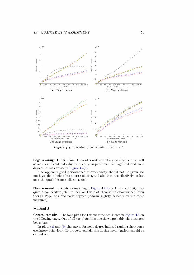
4.4. QUANTITATIVE ASSESSMENT 71
Number of removed edges GGGGGGA
Dev
iati
onGGGGGGA
0 200 400 600 800 1000 1200 1400 1600 1800 20000
1
2
3
4
5
6 ×10³
(a) Edge removal
Number of added edges GGGGGGA
Dev
iati
onGGGGGGA
0 200 400 600 800 1000 1200 1400 1600 1800 20000
0.5
1
1.5
2
2.5
3
3.5
4 ×10³
(b) Edge addition
Number of rewired edges GGGGGGA
Dev
iati
onGGGGGGA
0 200 400 600 800 1000 1200 1400 1600 1800 20000
0.2
0.4
0.6
0.8
1
1.2
1.4
1.6
1.8
2 ×10⁴
(c) Edge rewiring
Number of removed nodes GGGGGGA
Dev
iati
onGGGGGGA
0 10 20 30 40 50 60 70 80 90 1000
0.2
0.4
0.6
0.8
1
1.2 ×10³
(d) Node removal
Figure 4.4: Sensitivity for deviation measure 2.
Edge rewiring HITS, being the most sensitive ranking method here, as wellas status and centroid value are clearly outperformed by PageRank and nodedegrees, as we can see in Figure 4.4(c).
The apparent good performance of excentricity should not be given toomuch weight in light of its poor resolution, and also that it is effectively uselessonce the graph becomes disconnected.
Node removal The interesting thing in Figure 4.4(d) is that excentricity doesquite a competitive job. In fact, on this plot there is no clear winner (eventhough PageRank and node degrees perform slightly better than the othermeasures).
Method 3
General remarks The four plots for this measure are shown in Figure 4.5 onthe following page. Out of all the plots, this one shows probably the strangestbehaviors.
In plots (a) and (b) the curves for node degree induced ranking show someoscillatory behaviour. To properly explain this further investigations should becarried out.
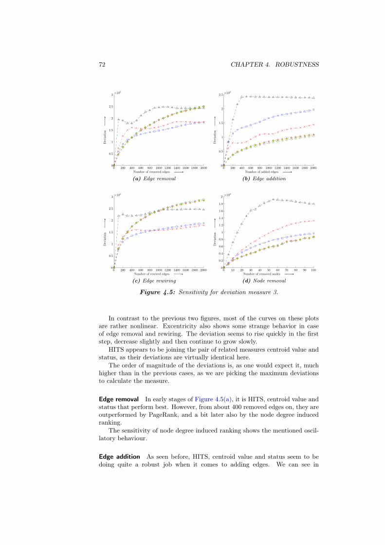
72 CHAPTER 4. ROBUSTNESS
Number of removed edges GGGGGGA
Dev
iati
onGGGGGGA
0 200 400 600 800 1000 1200 1400 1600 1800 20000
0.5
1
1.5
2
2.5
3 ×10⁵
(a) Edge removal
Number of added edges GGGGGGA
Dev
iati
onGGGGGGA
0 200 400 600 800 1000 1200 1400 1600 1800 20000
0.5
1
1.5
2
2.5 ×10⁵
(b) Edge addition
Number of rewired edges GGGGGGA
Dev
iati
onGGGGGGA
0 200 400 600 800 1000 1200 1400 1600 1800 20000
0.5
1
1.5
2
2.5
3 ×10⁵
(c) Edge rewiring
Number of removed nodes GGGGGGA
Dev
iati
onGGGGGGA
0 10 20 30 40 50 60 70 80 90 1000
0.2
0.4
0.6
0.8
1
1.2
1.4
1.6
1.8
2 ×10⁵
(d) Node removal
Figure 4.5: Sensitivity for deviation measure 3.
In contrast to the previous two figures, most of the curves on these plotsare rather nonlinear. Excentricity also shows some strange behavior in caseof edge removal and rewiring. The deviation seems to rise quickly in the firststep, decrease slightly and then continue to grow slowly.
HITS appears to be joining the pair of related measures centroid value andstatus, as their deviations are virtually identical here.
The order of magnitude of the deviations is, as one would expect it, muchhigher than in the previous cases, as we are picking the maximum deviationsto calculate the measure.
Edge removal In early stages of Figure 4.5(a), it is HITS, centroid value andstatus that perform best. However, from about 400 removed edges on, they areoutperformed by PageRank, and a bit later also by the node degree inducedranking.
The sensitivity of node degree induced ranking shows the mentioned oscil-latory behaviour.
Edge addition As seen before, HITS, centroid value and status seem to bedoing quite a robust job when it comes to adding edges. We can see in
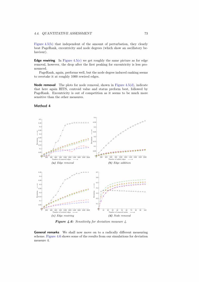
4.4. QUANTITATIVE ASSESSMENT 73
Figure 4.5(b) that independent of the amount of perturbation, they clearlybeat PageRank, excentricity and node degrees (which show an oscillatory be-haviour).
Edge rewiring In Figure 4.5(c) we get roughly the same picture as for edgeremoval, however, the drop after the first peaking for excentricity is less pro-nounced.
PageRank, again, performs well, but the node degree induced ranking seemsto overtake it at roughly 1000 rewired edges.
Node removal The plots for node removal, shown in Figure 4.5(d), indicatethat here again HITS, centroid value and status preform best, followed byPageRank. Excentricity is out of competition as it seems to be much moresensitive than the other measures.
Method 4
Number of removed edges GGGGGGA
Dev
iati
onGGGGGGA
0 200 400 600 800 1000 1200 1400 1600 1800 20000
0.05
0.1
0.15
0.2
0.25
0.3
0.35
0.4
0.45
0.5
(a) Edge removal
Number of added edges GGGGGGA
Dev
iati
onGGGGGGA
0 200 400 600 800 1000 1200 1400 1600 1800 20000
0.05
0.1
0.15
0.2
0.25
0.3
0.35
0.4
(b) Edge addition
Number of rewired edges GGGGGGA
Dev
iati
onGGGGGGA
0 200 400 600 800 1000 1200 1400 1600 1800 20000
0.05
0.1
0.15
0.2
0.25
0.3
0.35
0.4
0.45
(c) Edge rewiring
Number of removed nodes GGGGGGA
Dev
iati
onGGGGGGA
0 10 20 30 40 50 60 70 80 90 1000
0.1
0.2
0.3
0.4
0.5
0.6
0.7
(d) Node removal
Figure 4.6: Sensitivity for deviation measure 4.
General remarks We shall now move on to a radically different measuringscheme. Figure 4.6 shows some of the results from our simulations for deviationmeasure 4.
74 CHAPTER 4. ROBUSTNESS
The most homogeneous picture is obtained for edge addition, where all themeasures except excentricity are more or less equally good.
HITS again sticks quite closely to centroid value and status, PageRank andnode degrees perform well with roughly the same amount of deviation for eachof the different edge perturbations.
It is interesting to note that PageRank (and in a way also node degrees, ifwe neglect the oscillations) show quantitatively the same amount of sensitivityfor all three types of edge perturbations.
Edge removal Until up to 400 removed edges, excentricity and node de-gree seem to be better than the other ranking methods, as we can see inFigure 4.6(a). But beyond that point the node degree deviation shows someoscillations again. PageRank then seems to give the most consistent results.
Edge addition There is not much to note in Figure 4.6(b) other than thatexcentricity preforms poorly again, the other five measures seeming much morerobust. They perform roughly equally well, HITS being the best, on closeinspection.
Edge rewiring Similar to edge removal, three groups are apparent in Figure 4.6(c).That is, PageRank and node degrees perform best, followed by HITS, centroidvalue and status, and the rather sensitive excentricity.
Node removal In the case of node removal, Figure 4.6(d), after a fast increasein deviation the curves level out to a more slow increase. The excentricityinduced ranking seems to slowly decrease in sensitivity again after the initial“boost”, which should not be taken too serious in light of our earlier remarks.
Method 5
General remarks With minor differences, the in shapes of the subplots foredge removal and rewiring in Figure 4.7 on the facing page closely resembleeach other as well as to the corresponding ones from measure 1 (Figure 4.3(a) and (b) on page 67). Here, the shapes of the excentricity curves are verysimilar to the distribution of disconnected graphs, Figure 4.1 on page 65, whichcan be explained easily.
Besides the strong oscillations in the sensitivity of the node degree rankingin case of edge addition, both PageRank and node degree perform best in threeout of the four cases.
Edge removal The picture is quite clear in Figure 4.7(a), PageRank and nodedegrees being the methods of choice.
Edge addition Again, we find some oscillatory behaviour in the curve fornode degrees in Figure 4.7(b). The ranking induced by the nodes’ excentricitiesseems to be completely robust; next in line would be HITS followed closely bycentroid value and status.

4.4. QUANTITATIVE ASSESSMENT 75
Number of removed edges GGGGGGA
Dev
iati
onGGGGGGA
0 200 400 600 800 1000 1200 1400 1600 1800 20000
0.05
0.1
0.15
0.2
0.25
0.3
0.35
(a) Edge removal
Number of added edges GGGGGGA
Dev
iati
onGGGGGGA
0 200 400 600 800 1000 1200 1400 1600 1800 20000
0.02
0.04
0.06
0.08
0.1
0.12
0.14
0.16
0.18
0.2
(b) Edge addition
Number of rewired edges GGGGGGA
Dev
iati
onGGGGGGA
0 200 400 600 800 1000 1200 1400 1600 1800 20000
0.05
0.1
0.15
0.2
0.25
0.3
0.35
(c) Edge rewiring
Number of removed nodes GGGGGGA
Dev
iati
onGGGGGGA
0 10 20 30 40 50 60 70 80 90 1000
0.1
0.2
0.3
0.4
0.5
0.6
0.7
(d) Node removal
Figure 4.7: Sensitivity for deviation measure 5.
Edge rewiring The same comments as for edge removal can be made forFigure 4.7(c).
Node removal Clearly, Figure 4.7(d) is very similar to Figure 4.6(d), so wefind also for measure 5 that node degrees and PageRank allow for the leastsensitive ranking in case of node removal.
Method 6
General remarks It is not hard to see that excentricity does a very bad jobin all four cases of Figure 4.8 on the next page. The other measures performmuch better, if not ideally well: They appear to be completely robust withrespect to edge additions for instance as deviations there are actually zero.
PageRank seems one more time to be the overall winner, followed by nodedegrees.
Edge removal Besides the strong deviation for excentricity in Figure 4.8(a)(which can be explained by the disconnection issue again), HITS, centroid value
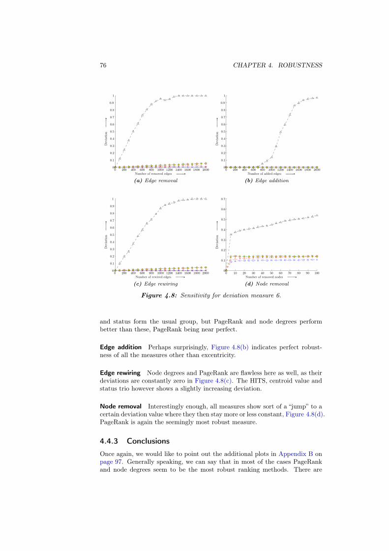
76 CHAPTER 4. ROBUSTNESS
Number of removed edges GGGGGGA
Dev
iati
onGGGGGGA
0 200 400 600 800 1000 1200 1400 1600 1800 20000
0.1
0.2
0.3
0.4
0.5
0.6
0.7
0.8
0.9
1
(a) Edge removal
Number of added edges GGGGGGA
Dev
iati
onGGGGGGA
0 200 400 600 800 1000 1200 1400 1600 1800 20000
0.1
0.2
0.3
0.4
0.5
0.6
0.7
0.8
0.9
1
(b) Edge addition
Number of rewired edges GGGGGGA
Dev
iati
onGGGGGGA
0 200 400 600 800 1000 1200 1400 1600 1800 20000
0.1
0.2
0.3
0.4
0.5
0.6
0.7
0.8
0.9
1
(c) Edge rewiring
Number of removed nodes GGGGGGA
Dev
iati
onGGGGGGA
0 10 20 30 40 50 60 70 80 90 1000
0.1
0.2
0.3
0.4
0.5
0.6
0.7
(d) Node removal
Figure 4.8: Sensitivity for deviation measure 6.
and status form the usual group, but PageRank and node degrees performbetter than these, PageRank being near perfect.
Edge addition Perhaps surprisingly, Figure 4.8(b) indicates perfect robust-ness of all the measures other than excentricity.
Edge rewiring Node degrees and PageRank are flawless here as well, as theirdeviations are constantly zero in Figure 4.8(c). The HITS, centroid value andstatus trio however shows a slightly increasing deviation.
Node removal Interestingly enough, all measures show sort of a “jump” to acertain deviation value where they then stay more or less constant, Figure 4.8(d).PageRank is again the seemingly most robust measure.
4.4.3 Conclusions
Once again, we would like to point out the additional plots in Appendix B onpage 97. Generally speaking, we can say that in most of the cases PageRankand node degrees seem to be the most robust ranking methods. There are
4.5. THEORETICAL RESULTS 77
however cases, where HITS as well as centroid value and status challenge thisposition, this happening most frequently at edge adding and node removingperturbations.
With the sensitivity varying from measure to measure it is hard to give ageneral recommendation, even without taking into account the actual useful-ness of the produced rankings themselves. In other words: the best schemestrongly depends on the question asked.
Before closing this chapter, let us quickly mention two theoretical results onsensitivity.
4.5 Theoretical results
As a complement to the extensive quantitative assessment of sensitivity wewould now like to present two theoretical results, one on HITS and one onPageRank, which have been published in a paper by Ng et al., [51].
4.5.1 Sensitivity of HITS
They claim (and prove) that the stability of the HITS algorithm is governed bythe so–called eigengap of the authority matrix, that is the difference betweenthe largest and the second largest eigenvalue of ATA.
This is done through the following theorem, which is unfortunately onlylimited to very small perturbations, that is addition or removal of a number ofedges to/from exactly one node.
Theorem 4.1 (Sensitivity of the HITS algorithm)Let A be the adjacency matrix of a graph G = (V, E), and M = ATA
be its associated authority matrix with principal eigenvector ν1 and eigengapη = λ1 − λ2. Assume the maximum out–degree of every node of G is boundedby kmax.
For any ε > 0, suppose we perturb G by adding or deleting at most k linksfrom one node, where
k <(
√
kmax + α−√
kmax
)2
, where α =εη
4 +√
2ε
Then
‖ν1 − ν1‖2 ≤ ε
holds for the perturbed principal eigenvector λ1 of the perturbed matrix M .
Proof: [51]. �
As we know from Subsection 3.3.2 on page 40, the principal eigenvectorcontains the hub scores of the network, so as little a change as possible in itis desired. However, knowing a bound on the amount of change in this vector
78 CHAPTER 4. ROBUSTNESS
does not imply a bound on the deviation of the ranking the scores induce. Itis therefore hard to draw further conclusions from this result.
The same limitation is also valid for their result on PageRank, which wedescribe now.
4.5.2 Sensitivity of PageRank
Stated in the same paper, the following theorem by Ng et al. is significantlyless restrictive than the one for HITS:
Theorem 4.2 (Sensitivity of the PageRank algorithm)Let P be the transition matrix of a graph G = (V, E) and πT be the principal
left hand eigenvector of ¯P = αP + (1− α)1n×n/n. Let nodes v1, v2, . . . , vm be
changed in any way and let ˜P be the resulting (new) transition matrix.
Then the new PageRank scores πT satisfy
‖πT − πT ‖1 ≤2∑m
i=1 πvi
1− α
where πvidenotes the PageRank score of node vi.
Proof: [51]. �
So, the impact of the perturbation depends on the nodes that are perturbed,and on the “damping factor” α chosen.
It is quite intuitive that the more important the perturbed nodes were inthe first place, the bigger the deviation will be resulting from the perturbation.Just think of the internet surfer illustration from above — the more importanta page is, the more frequent it will be visited, hence the greater the overallimpact of any change to it.
This is another aspect of the dilemma related to α (see Subsection 3.4.3 onpage 47). Here as well, one is tempted to lower it as it will certainly decreasesensitivity to perturbations. This becomes most obvious in the radical caseof setting α = 0. Here, the PageRank algorithm would run purely on thestatic 1/n matrix, completely ignoring any change in the transition matrixthat represents the graph.5
4.5.3 Limitations
Simulations not displayed here have shown that the bounds are very conser-vative. The actual deviation was usually by at least one order of magnitudesmaller than the bound.
But most importantly, both results have a major limitation: they only givebounds for a norm of the difference of the score vectors, not the resultingranking. As this is what we are interested in in our context we have little usehere for the theorems.
They are however a good start and point in the right direction, and furtherinvestigations should be carried out on this topic.
5 This also implies that the bound is not tight.

4.5. THEORETICAL RESULTS 79
We also noticed that both bounds are very crude. For example the effectivedeviations resulting from all meaningful perturbations we could inflict on var-ious types of graphs were roughly ten times smaller than the bound given inTheorem 4.2 on the preceding page, indicating that the bound could certainlybe improved with further investigation.
Now that we have an idea of the ranking schemes’ robustness with respectto differnet perturbations we shall investigate the actual correlation betweenattributed importance through high ranking and importance in the context ofan application, such as protein–protein interaction networks.

C H A P T E R 5
Application to real data
After analysing three real world networks we
evaluate the ranking schemes’ ability on them to
identify essential nodes, as well as the robustness of
this ability with respect to wrong data.
5.1 Introduction
In the previous chapters we have examined a number of ranking schemes andstudied their properties on computer generated networks. However, we havenot yet looked at how well these schemes actually identify “important” nodesin real world networks.
Of course, the precise interpretation of “important” depends on the appli-cation considered. For that reason, we look in this chapter at the possible ap-plication of ranking algorithms to biological networks, namely protein–proteininteraction networks.
Even in small and simple organism there are easily thousands of proteinsactive in a single cell. Proteins can be enzymes directly involved in chemicalreactions of the metabolism, or can be part of larger modules like ribosomes ormitochondria. Other types of proteins are involved in regulation and controlof gene expression, or serve as messengers that signal between cells.
For many applications it is crucial to understand the interactions betweenthe proteins in living cells. One approach biologists have taken is to establishso called protein–protein interaction networks which allow an effective analysisof the system of interactions. In these networks, proteins form the nodes, andthey are linked together if they interact in some way or other, resulting in anundirected graph.
With more and more datasets becoming available we shall evaluate theperformance of our ranking schemes in identifying essential nodes.1 We usethree recent datasets, namely those from Uetz et al. [59], Yu et al. [64] and Itoet al. [32].2 These datasets provide us with the actual networks and also witha list of proteins known to be essential.
After examining the networks we will evaluate the fraction of essential nodesamong a certain top fraction of nodes in the different rankings, as well as therobustness of the identification process with respect to perturbations in thenetworks.
1 A protein is considered essential if its removal causes the organism to die.2 Although the data itself has been taken from the accompanying website of the article
by Uetz et al. [64]: http://bioinfo.mbb.yale.edu/network/essen/ .
81
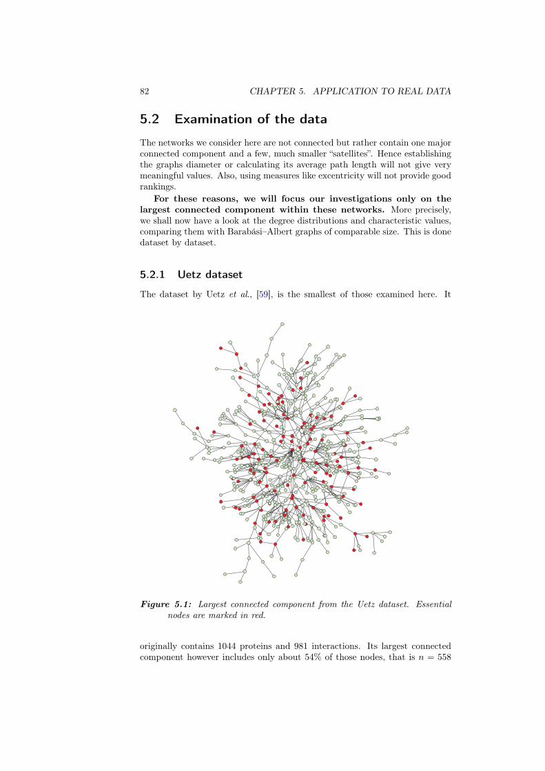
82 CHAPTER 5. APPLICATION TO REAL DATA
5.2 Examination of the data
The networks we consider here are not connected but rather contain one majorconnected component and a few, much smaller “satellites”. Hence establishingthe graphs diameter or calculating its average path length will not give verymeaningful values. Also, using measures like excentricity will not provide goodrankings.
For these reasons, we will focus our investigations only on the
largest connected component within these networks. More precisely,we shall now have a look at the degree distributions and characteristic values,comparing them with Barabási–Albert graphs of comparable size. This is donedataset by dataset.
5.2.1 Uetz dataset
The dataset by Uetz et al., [59], is the smallest of those examined here. It
Figure 5.1: Largest connected component from the Uetz dataset. Essentialnodes are marked in red.
originally contains 1044 proteins and 981 interactions. Its largest connectedcomponent however includes only about 54% of those nodes, that is n = 558
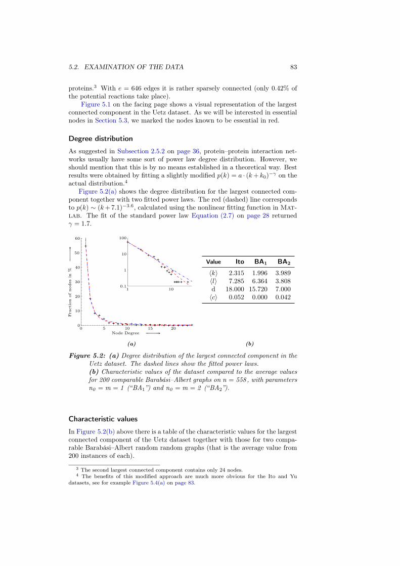
5.2. EXAMINATION OF THE DATA 83
proteins.3 With e = 646 edges it is rather sparsely connected (only 0.42% ofthe potential reactions take place).
Figure 5.1 on the facing page shows a visual representation of the largestconnected component in the Uetz dataset. As we will be interested in essentialnodes in Section 5.3, we marked the nodes known to be essential in red.
Degree distribution
As suggested in Subsection 2.5.2 on page 36, protein–protein interaction net-works usually have some sort of power law degree distribution. However, weshould mention that this is by no means established in a theoretical way. Bestresults were obtained by fitting a slightly modified p(k) = a · (k + k0)
−γ on theactual distribution.4
Figure 5.2(a) shows the degree distribution for the largest connected com-ponent together with two fitted power laws. The red (dashed) line correspondsto p(k) ∼ (k +7.1)−3.6, calculated using the nonlinear fitting function in Mat-
lab. The fit of the standard power law Equation (2.7) on page 28 returnedγ = 1.7.
Node Degree GGGGGGGGGGA
Fractio
nofnodes
in%
GGGGGGGGGGA
1 10
0 5 10 15 20
0.1
1
10
100
0
10
20
30
40
50
60
(a)
Value Ito BA1 BA2
〈k〉 2.315 1.996 3.989〈l〉 7.285 6.364 3.808d 18.000 15.720 7.000〈c〉 0.052 0.000 0.042
(b)
Figure 5.2: (a) Degree distribution of the largest connected component in theUetz dataset. The dashed lines show the fitted power laws.(b) Characteristic values of the dataset compared to the average valuesfor 200 comparable Barabási–Albert graphs on n = 558 , with parametersn0 = m = 1 (“BA1”) and n0 = m = 2 (“BA2”).
Characteristic values
In Figure 5.2(b) above there is a table of the characteristic values for the largestconnected component of the Uetz dataset together with those for two compa-rable Barabási–Albert random random graphs (that is the average value from200 instances of each).
3 The second largest connected component contains only 24 nodes.4 The benefits of this modified approach are much more obvious for the Ito and Yu
datasets, see for example Figure 5.4(a) on page 83.

84 CHAPTER 5. APPLICATION TO REAL DATA
The Barabási–Albert model used had n = 558 and n0 = m = 1 (column“BA1”). This gave the fixed power law exponent γ = 3 and e = 557 edges(compared to 646 edges in the dataset). Using n0 = m = 2 (column “BA2”) weobtain graphs with about twice as many edges, e = 1113.
It is the lack of edges in the “BA1” case that explains the smaller averagenode degree compared to the dataset. The missing clustering is due to thespecific generating algorithm (which cannot produce any “triangles” startingwith only one node and adding 1 edge with each new node). It is interestingto see, however, that average path length and diameter are smaller — even ifthere are less edges in total. This means, that the pure Barabási–Albert modelcreates more efficiently connected graphs.
The much denser “BA2” setup also fails to properly reflect the propertiesof the dataset as it is significantly denser. Even so, clustering is lower than inthe original data, indicating that the biological network is quite clustered.
5.2.2 Ito dataset
We now take a look at the next larger dataset, namely the one by Ito et al.,[32].
Figure 5.3: Largest connected component from the Ito dataset. Essentialnodes are marked in red.

5.2. EXAMINATION OF THE DATA 85
It contains a total of 3278 nodes and 4393 edges. Again, the correspond-ing graph is disconnected and contains one dominating cluster. This largestconnected component contains about 87% of the proteins, that is n = 2840.5
A total of e = 4147 edges within that component make it the sparsest of thethree networks, as only 0.10% of the possible edges are present.
Even so, the visual representation of the network, Figure 5.3 on the preced-ing page, looks rather dense. Essential nodes are, again, coloured red.
Degree distribution
We show in Figure 5.4(a) below the degree distribution for the largest con-nected component of the Ito dataset as well as fitted power laws. The bestfit was obtained using the modified power law (red dashed line), resulting inp(k) ∼ (k + 5.1)−4.7. The pure power law resulted in an exponent of γ = 1.4(blue dash–dotted line).
Node Degree GGGGGGGGGGA
Fractio
nofnodes
in%
GGGGGGGGGGA
1 10 100
0 50 100 150 200 250
0.1
1
10
100
0
5
10
15
20
25
30
35
40
45
50
(a)
Value Ito BA1 BA2
〈k〉 2.920 1.999 3.997〈l〉 4.886 7.972 4.514d 14.000 20.630 8.010〈c〉 0.038 0.000 0.012
(b)
Figure 5.4: (a) Degree distribution of the largest connected component in theIto dataset. The dashed lines show the fitted power laws.(b) Characteristic values of the dataset compared to the average valuesfor 200 comparable Barabási–Albert graphs on n = 2840 , with parame-ters n0 = m = 1 (“BA1”) and n0 = m = 2 (“BA2”).
Characteristic values
The table in Figure 5.4(b) above shows the results from the analysis of the realdata as well as two attempts to imitate its properties with a scale–free graph.
As the number of edges of the real graph (more precisely of the largest con-nected component) falls exactly between the number of edges possible with thestandard Barabási–Albert model, we present, again, two different parametercombinations (that is n0 = m = 1 and n0 = m = 2), resulting respectively ingraphs with e = 2839 (column “BA1”) and e = 5677 (columns “BA2”).
We observe similar behavior as for the Uetz dataset: for the sparser graphs(“BA1”), the average node degree is, of course, lower and clustering is zero. The
5 All other connected component have equal or less than 6 nodes.
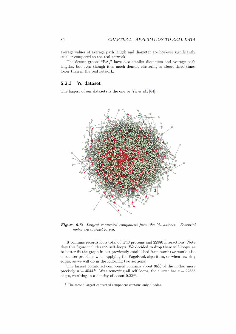
86 CHAPTER 5. APPLICATION TO REAL DATA
average values of average path length and diameter are however significantlysmaller compared to the real network.
The denser graphs “BA2” have also smaller diameters and average pathlengths, but even though it is much denser, clustering is about three timeslower than in the real network.
5.2.3 Yu dataset
The largest of our datasets is the one by Yu et al., [64].
Figure 5.5: Largest connected component from the Yu dataset. Essentialnodes are marked in red.
It contains records for a total of 4743 proteins and 22980 interactions. Notethat this figure includes 629 self–loops. We decided to drop these self–loops, asto better fit the graph in our previously established framework (we would alsoencounter problems when applying the PageRank algorithm, or when rewiringedges, as we will do in the following two sections).
The largest connected component contains about 96% of the nodes, moreprecisely n = 4544.6 After removing all self–loops, the cluster has e = 22588edges, resulting in a density of about 0.22%.
6 The second largest connected component contains only 4 nodes.
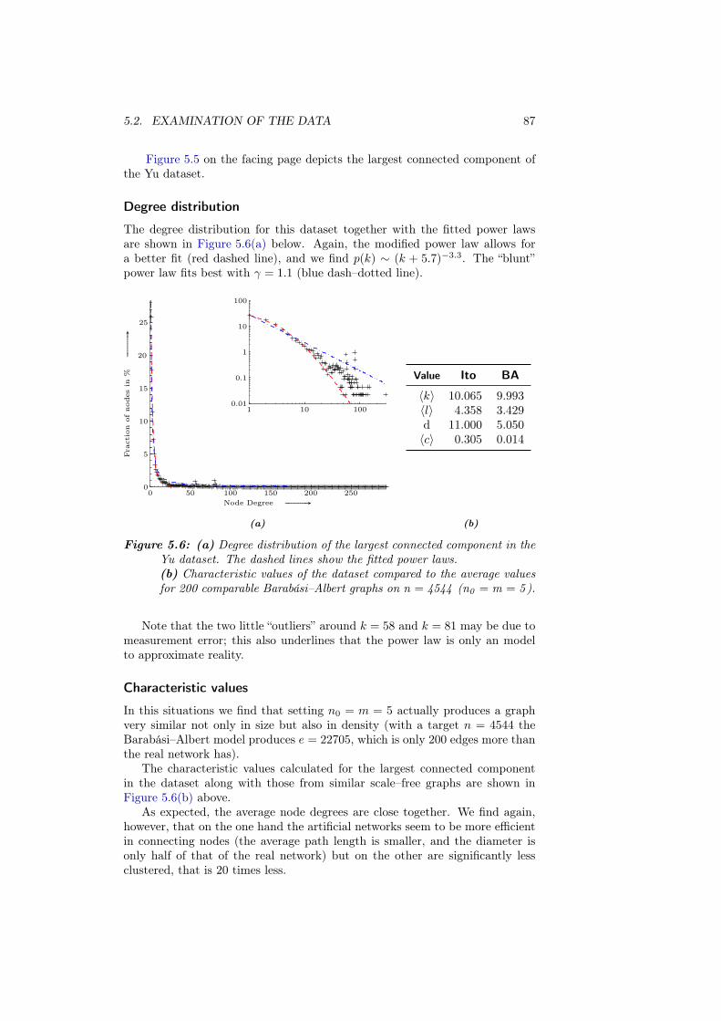
5.2. EXAMINATION OF THE DATA 87
Figure 5.5 on the facing page depicts the largest connected component ofthe Yu dataset.
Degree distribution
The degree distribution for this dataset together with the fitted power lawsare shown in Figure 5.6(a) below. Again, the modified power law allows fora better fit (red dashed line), and we find p(k) ∼ (k + 5.7)−3.3. The “blunt”power law fits best with γ = 1.1 (blue dash–dotted line).
Node Degree GGGGGGGGGGA
Fractio
nofnodes
in%
GGGGGGGGGGA
1 10 100
0 50 100 150 200 250
0.01
0.1
1
10
100
0
5
10
15
20
25
(a)
Value Ito BA
〈k〉 10.065 9.993〈l〉 4.358 3.429d 11.000 5.050〈c〉 0.305 0.014
(b)
Figure 5.6: (a) Degree distribution of the largest connected component in theYu dataset. The dashed lines show the fitted power laws.(b) Characteristic values of the dataset compared to the average valuesfor 200 comparable Barabási–Albert graphs on n = 4544 (n0 = m = 5 ).
Note that the two little “outliers” around k = 58 and k = 81 may be due tomeasurement error; this also underlines that the power law is only an modelto approximate reality.
Characteristic values
In this situations we find that setting n0 = m = 5 actually produces a graphvery similar not only in size but also in density (with a target n = 4544 theBarabási–Albert model produces e = 22705, which is only 200 edges more thanthe real network has).
The characteristic values calculated for the largest connected componentin the dataset along with those from similar scale–free graphs are shown inFigure 5.6(b) above.
As expected, the average node degrees are close together. We find again,however, that on the one hand the artificial networks seem to be more efficientin connecting nodes (the average path length is smaller, and the diameter isonly half of that of the real network) but on the other are significantly lessclustered, that is 20 times less.
88 CHAPTER 5. APPLICATION TO REAL DATA
5.2.4 Conclusions
All three models had in common that their degree distribution deviates quiteclearly from a pure power law distribution, but a slight modification can im-prove the fit.
The networks based on the real data all show a significantly higher clus-tering than the ones created by the Barabási–Albert model. These, however,feature shorter average path lengths and a smaller diameter.
With the three datasets introduced we shall now continue by investigating theperformance of our ranking schemes in identifying biologically essential nodes.
5.3 Identifying essentiality
In the third chapter we presented a number of ranking schemes and motivatedtheir use. Chapter 4 then investigated their robustness with respect to wrongor missing data using artificial networks of the Barabási–Albert type. We nowexamine the biological relevance of the different notions of importance. Inparticular, we consider question of the type “If a node is PageRank–important,is it also essential for the survival of the organism?”
We will try give an answer to this type of question by examining the overlapor intersection of nodes identified as important by our ranking schemes andnodes known to be essential (from a biological point of view). This is done,again, dataset by dataset.
5.3.1 Our setup
In the following we shall not take into account the actual rank of the nodes, aswe have only the “binary” information whether a protein is essential or not. Infact, we proceed similar to deviation measure 4 from the previous chapter.
Calculation of quality
Recall Table 4.1(d) on page 60, with the sets IO and IP , and think of them,now, as being respectively the set of “known–to–be–essential”–nodes and theset of “thought–to–be–important”–nodes given by the ranking scheme.7
The set of essential nodes I0 is given along with the datasets; IP is obtainedby taking a certain percentile of the most highly ranked nodes. The issue ofties is dealt with in the following way.
In looking at the intersection of both sets we get the number of correctlyidentified nodes. We then normalize that number by the total number of nodesin IP as to get the fraction of essential nodes among the “thought–to–be–important” nodes — and also to tackle the effect of including the ties. So thehigher the value |IO ∩ IP |/|IP |, the better the ranking scheme performs.
The general benchmark for the different ranking schemes is the global frac-tion of essential nodes in each network. This threshold lies around 20% ofthe nodes in each graph, so if one randomly picks, say, 5% of the nodes, thenroughly every fifth node should be essential.
7 Dropping the notion of perturbation for the moment.
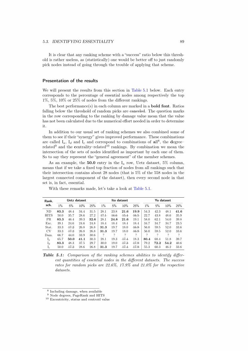
5.3. IDENTIFYING ESSENTIALITY 89
It is clear that any ranking scheme with a “success” ratio below this thresh-old is rather useless, as (statistically) one would be better off to just randomlypick nodes instead of going through the trouble of applying that scheme.
Presentation of the results
We will present the results from this section in Table 5.1 below. Each entrycorresponds to the percentage of essential nodes among respectively the top1%, 5%, 10% or 25% of nodes from the different rankings.
The best performance(s) in each column are marked in a bold font. Ratiosfalling below the threshold of random picks are canceled. The question marksin the row corresponding to the ranking by damage value mean that the valuehas not been calculated due to the numerical effort needed in order to determineit.
In addition to our usual set of ranking schemes we also combined some ofthem to see if their “synergy” gives improved performance. These combinationsare called Ia, Id and Ic and correspond to combinations of all8, the degree–related9 and the centrality–related10 rankings. By combination we mean theintersection of the sets of nodes identified as important by each one of them.So to say they represent the “general agreement” of the member schemes.
As an example, the 50.0 entry in the Ia row, Uetz dataset, 5% column,means that if we take a fixed top fraction of nodes from all rankings such thattheir intersection contains about 28 nodes (that is 5% of the 558 nodes in thelargest connected component of the dataset), then every second node in thatset is, in fact, essential.
With these remarks made, let’s take a look at Table 5.1.
Uetz dataset Ito dataset Yu datasetRank.sch. 1% 5% 10% 25% 1% 5% 10% 25% 1% 5% 10% 25%
ND 83.3 48.4 34.4 31.5 28.1 23.8 21.6 19.9 54.3 42.3 48.1 41.6
HITS 50.0 35.7 28.6 27.2 17.1 16.6 15.4 16.5 22.7 43.8 48.6 35.9PR 83.3 46.4 39.3 32.6 28.1 24.8 21.6 19.1 58.0 62.1 54.0 39.8Exc. 39.1 24.6 24.6 24.8 18.4 18.4 18.4 18.4 34.7 34.7 34.7 23.5Stat. 33.3 17.2 26.8 26.8 31.3 19.7 18.0 16.9 56.0 59.5 52.0 33.6CV 33.3 17.2 26.8 26.8 31.3 19.7 18.0 16.9 56.0 59.5 52.0 33.6
Dam. 66.7 44.0 33.9 30.6 ? ? ? ? ? ? ? ?Ia 65.7 50.0 41.1 30.3 28.1 19.3 17.4 18.3 80.4 68.4 51.8 39.7Id 83.3 48.3 37.5 29.7 30.0 19.0 17.3 17.9 79.2 72.2 54.2 40.6Ic 50.0 17.2 28.6 26.8 31.3 19.7 17.4 17.9 55.3 60.3 46.2 33.6
Table 5.1: Comparison of the ranking schemes abilities to identify differ-ent quantities of essential nodes in the different datasets. The successrates for random picks are 22.6%, 17.9% and 21.0% for the respectivedatasets.
8 Including damage, when available9 Node degrees, PageRank and HITS
10 Excentricity, status and centroid value
90 CHAPTER 5. APPLICATION TO REAL DATA
5.3.2 Uetz dataset
The results for this dataset look quite convincing (with the exception of thedrop in performance of the status and centroid value induced rankings at 5%)and in a way intuitive: Generally, all ranking schemes decrease in performanceas we ask for more and more important nodes. This makes sense, because themore nodes we demand, the more likely it will be that ranking scheme andreality “disagree”; whereas if we only want a handful of the most importantnodes, the vast majority of them should (hopefully) be essential.
In this dataset, the global fraction of essential nodes is 22.6%. When weask only for a few nodes, node degrees and PageRank share the first place,together with Id (their combination with HITS). Demanding for larger numbersof important nodes, it is the combination of all rankings schemes Ia that has thehighest success rate, about one in two are correctly identified. If we consideran even larger fraction, a quarter of the nodes, about one third of the nodesidentified by PageRank are essential.
In any case, status, centroid value and excentricity perform worst, whereasin contrast the combination of all of the schemes gives consistently good results.In a way surprising, damage also performs quite well, at least better than anyof the centrality based ranking schemes.
5.3.3 Ito dataset
The situation is quite different in this dataset, as excentricity, status and cen-troid value perform better relative to PageRank and node degrees than in theprevious case. However, the latter two again allow for the highest success rateswhen we ask for more than 140 proteins (5% of the network size).
The benchmark of 17.9% in case of random picks is however crossed anumber of times — and, surprisingly, HITS lies entirely below it. In case ofdesired 10 and 25% of nodes, status and centroid value are not doing well(contrary to their good performance for the very top ranked 1% of nodes).
Probably due to their low fraction of essential nodes, all the combinationmethods fail as well to deliver better results than just randomly picking nodes.
Excentricity performs also quite bad, and the constant values due to thefact, again, that the ranking induced by the excentricities of the nodes is ex-tremely clustered.
5.3.4 Yu dataset
The first thing we would like to point out is that we can confirm the resultfrom the paper by Yu et al. [64]. They defined 1061 nodes (around 22% ofthe total network size) of the most highly connected nodes as hubs, and foundthat about 43% of them are essential. In taking about 25% of the nodes withthe highest degrees this fraction is has decreased slightly to about 41.6%. Thisis in agreement with their prediction in the supplementary material to theirpaper [65].
Containing 953 essential nodes, about 21% of randomly picked nodes (fromthe largest connected component) should be essential. It is positive to see that,unlike the Ito dataset, this threshold is not crossed here.
5.4. ROBUSTNESS OF THE IDENTIFICATION OF ESSENTIALITY 91
Most notable is, however, that again the combination of all ranking schemesor just the degree based schemes provide best results in this dataset. However,status and centroid value also allow for more than a third of correctly identifiednodes.
Strangely again, HITS gives a very bad result when we look at the very topranked nodes, but then increases to come close to a 50% success rate.
5.3.5 Comparison between the datasets
In general, all ranking schemes work best on the Uetz dataset, correctly iden-tifying at least one fifth of nodes (except for the one case of centroid value andstatus). We also find the highest ratio, that is 83.3% of essential nodes amongthe top scoring nodes with respect to node degrees and PageRank.
Good results are also obtained for the large dataset by Yu et al.. With twosmall exceptions, at least a third of the nodes are correctly identified, and inthe majority of cases even more than 50%.
Maybe due to the quality of the data and lacking robustness in the rankingschemes, they perform not as well on the Ito dataset. Here, at most a third ofthe identified nodes are essential. Some rankings schemes even drop below thethreshold where one would be better off to just randomly pick nodes.
Among the different schemes, it is again the centrality based ones that per-form worst. Damage however seems to work quite well, at least on the Uetzdataset. Further investigations might show whether this will also be the casefor other dataset. It is doubtful though that the quality of the results will beable to justify the disproportionately higher computational effort.
Having examined the ability of the different ranking schemes to identify es-sential nodes in the datasets, we would like to close this last chapter by testingthe robustness of this identification process.
5.4 Robustness of the identification of
essentiality
Some of the strange effects from the previous section, like the sudden but“temporary” collapse of the values from centroid value and status at 5% in theUetz dataset, can surely be explained by the considerable amount of noise inthe datasets.
To further investigate the effect of perturbations on the rankings we madeanother series of simulations.
5.4.1 Our setup
We introduced different amounts (5%, 10%, 15% and 20% of the number ofedges) of edge perturbations (removal, rewiring and addition) to each of thedatasets and averaged over 50 runs.
The results are presented in a similar manner as in the previous section, withthe important difference that the percentages in the table head now correspondto the amount of perturbation introduced. As in the previous chapter for
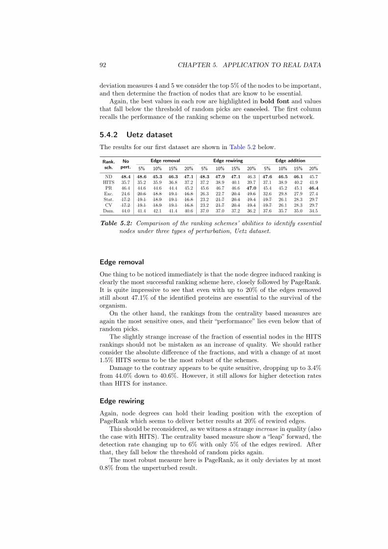
92 CHAPTER 5. APPLICATION TO REAL DATA
deviation measures 4 and 5 we consider the top 5% of the nodes to be important,and then determine the fraction of nodes that are know to be essential.
Again, the best values in each row are highlighted in bold font and valuesthat fall below the threshold of random picks are canceled. The first columnrecalls the performance of the ranking scheme on the unperturbed network.
5.4.2 Uetz dataset
The results for our first dataset are shown in Table 5.2 below.
Edge removal Edge rewiring Edge additionRank.sch.
Nopert. 5% 10% 15% 20% 5% 10% 15% 20% 5% 10% 15% 20%
ND 48.4 48.6 45.3 46.3 47.1 48.3 47.9 47.1 46.3 47.6 46.5 46.1 45.7HITS 35.7 35.2 35.9 36.8 37.2 37.2 38.9 40.1 39.7 37.1 38.9 40.2 41.9PR 46.4 44.6 44.6 44.4 45.2 45.6 46.7 46.6 47.0 45.4 45.2 45.1 46.4
Exc. 24.6 20.6 18.8 19.1 16.8 26.3 22.7 20.4 19.6 32.6 29.8 27.9 27.4Stat. 17.2 19.1 18.9 19.1 16.8 23.2 21.7 20.4 19.4 19.7 26.1 28.3 29.7CV 17.2 19.1 18.9 19.1 16.8 23.2 21.7 20.4 19.4 19.7 26.1 28.3 29.7
Dam. 44.0 41.4 42.1 41.4 40.6 37.0 37.0 37.2 36.2 37.6 35.7 35.0 34.5
Table 5.2: Comparison of the ranking schemes’ abilities to identify essentialnodes under three types of perturbation, Uetz dataset.
Edge removal
One thing to be noticed immediately is that the node degree induced ranking isclearly the most successful ranking scheme here, closely followed by PageRank.It is quite impressive to see that even with up to 20% of the edges removedstill about 47.1% of the identified proteins are essential to the survival of theorganism.
On the other hand, the rankings from the centrality based measures areagain the most sensitive ones, and their “performance” lies even below that ofrandom picks.
The slightly strange increase of the fraction of essential nodes in the HITSrankings should not be mistaken as an increase of quality. We should ratherconsider the absolute difference of the fractions, and with a change of at most1.5% HITS seems to be the most robust of the schemes.
Damage to the contrary appears to be quite sensitive, dropping up to 3.4%from 44.0% down to 40.6%. However, it still allows for higher detection ratesthan HITS for instance.
Edge rewiring
Again, node degrees can hold their leading position with the exception ofPageRank which seems to deliver better results at 20% of rewired edges.
This should be reconsidered, as we witness a strange increase in quality (alsothe case with HITS). The centrality based measure show a “leap” forward, thedetection rate changing up to 6% with only 5% of the edges rewired. Afterthat, they fall below the threshold of random picks again.
The most robust measure here is PageRank, as it only deviates by at most0.8% from the unperturbed result.
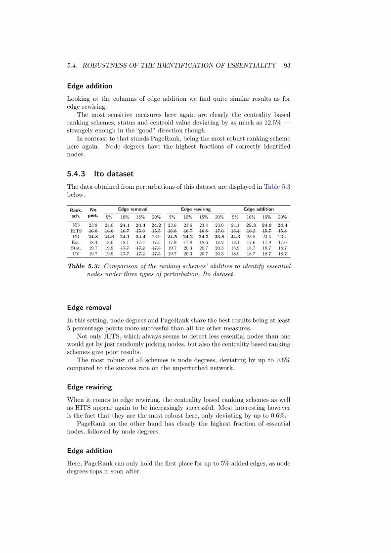
5.4. ROBUSTNESS OF THE IDENTIFICATION OF ESSENTIALITY 93
Edge addition
Looking at the columns of edge addition we find quite similar results as foredge rewiring.
The most sensitive measures here again are clearly the centrality basedranking schemes, status and centroid value deviating by as much as 12.5% —strangely enough in the “good” direction though.
In contrast to that stands PageRank, being the most robust ranking schemehere again. Node degrees have the highest fractions of correctly identifiednodes.
5.4.3 Ito dataset
The data obtained from perturbations of this dataset are displayed in Table 5.3below.
Edge removal Edge rewiring Edge additionRank.sch.
Nopert. 5% 10% 15% 20% 5% 10% 15% 20% 5% 10% 15% 20%
ND 23.8 24.0 24.1 24.4 24.2 23.6 23.6 23.4 23.0 24.1 25.3 24.9 24.4
HITS 16.6 16.6 16.7 15.9 15.5 16.8 16.7 16.8 17.0 16.4 16.2 15.7 15.8PR 24.8 24.6 24.1 24.4 23.9 24.5 24.2 24.2 23.8 24.3 23.8 23.5 23.4Exc. 18.4 18.0 18.1 17.4 17.5 17.9 17.8 18.6 18.2 18.1 17.6 17.9 17.6Stat. 19.7 19.9 17.7 17.2 17.5 19.7 20.3 20.7 20.3 18.9 18.7 18.7 18.7CV 19.7 19.9 17.7 17.2 17.5 19.7 20.3 20.7 20.3 18.9 18.7 18.7 18.7
Table 5.3: Comparison of the ranking schemes’ abilities to identify essentialnodes under three types of perturbation, Ito dataset.
Edge removal
In this setting, node degrees and PageRank share the best results being at least5 percentage points more successful than all the other measures.
Not only HITS, which always seems to detect less essential nodes than onewould get by just randomly picking nodes, but also the centrality based rankingschemes give poor results.
The most robust of all schemes is node degrees, deviating by up to 0.6%compared to the success rate on the unperturbed network.
Edge rewiring
When it comes to edge rewiring, the centrality based ranking schemes as wellas HITS appear again to be increasingly successful. Most interesting howeveris the fact that they are the most robust here, only deviating by up to 0.6%.
PageRank on the other hand has clearly the highest fraction of essentialnodes, followed by node degrees.
Edge addition
Here, PageRank can only hold the first place for up to 5% added edges, as nodedegrees tops it soon after.
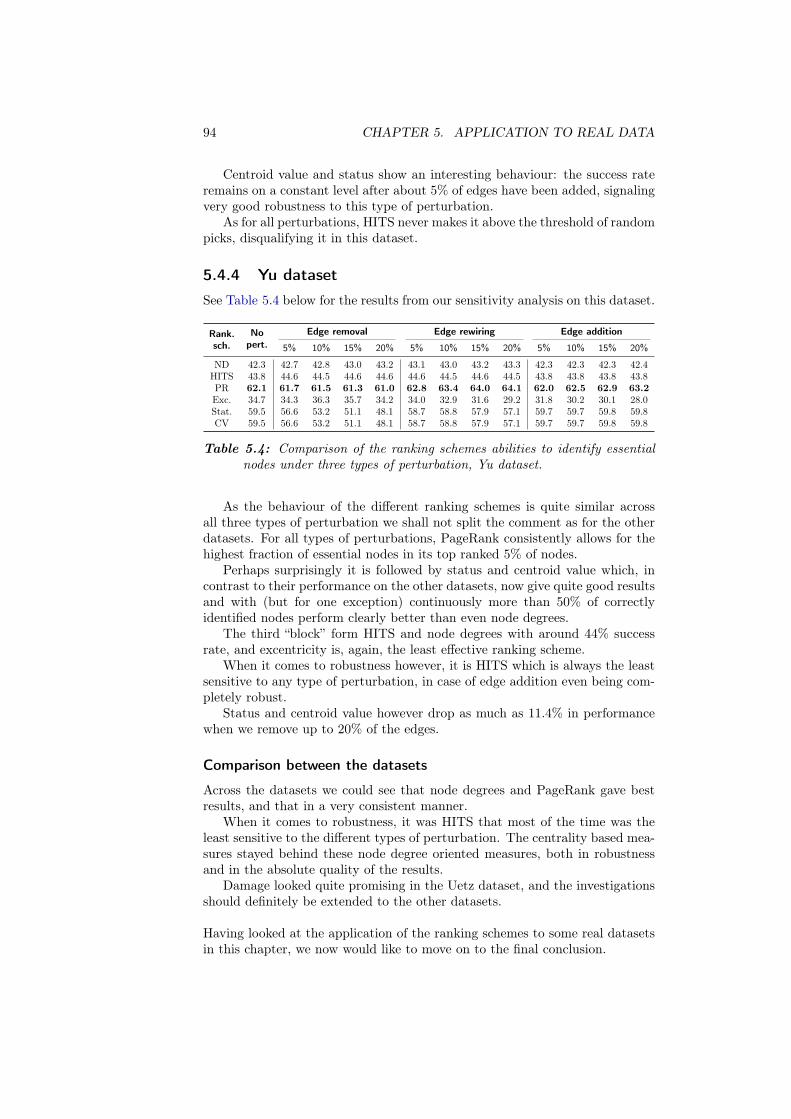
94 CHAPTER 5. APPLICATION TO REAL DATA
Centroid value and status show an interesting behaviour: the success rateremains on a constant level after about 5% of edges have been added, signalingvery good robustness to this type of perturbation.
As for all perturbations, HITS never makes it above the threshold of randompicks, disqualifying it in this dataset.
5.4.4 Yu dataset
See Table 5.4 below for the results from our sensitivity analysis on this dataset.
Edge removal Edge rewiring Edge additionRank.sch.
Nopert. 5% 10% 15% 20% 5% 10% 15% 20% 5% 10% 15% 20%
ND 42.3 42.7 42.8 43.0 43.2 43.1 43.0 43.2 43.3 42.3 42.3 42.3 42.4HITS 43.8 44.6 44.5 44.6 44.6 44.6 44.5 44.6 44.5 43.8 43.8 43.8 43.8PR 62.1 61.7 61.5 61.3 61.0 62.8 63.4 64.0 64.1 62.0 62.5 62.9 63.2
Exc. 34.7 34.3 36.3 35.7 34.2 34.0 32.9 31.6 29.2 31.8 30.2 30.1 28.0Stat. 59.5 56.6 53.2 51.1 48.1 58.7 58.8 57.9 57.1 59.7 59.7 59.8 59.8CV 59.5 56.6 53.2 51.1 48.1 58.7 58.8 57.9 57.1 59.7 59.7 59.8 59.8
Table 5.4: Comparison of the ranking schemes abilities to identify essentialnodes under three types of perturbation, Yu dataset.
As the behaviour of the different ranking schemes is quite similar acrossall three types of perturbation we shall not split the comment as for the otherdatasets. For all types of perturbations, PageRank consistently allows for thehighest fraction of essential nodes in its top ranked 5% of nodes.
Perhaps surprisingly it is followed by status and centroid value which, incontrast to their performance on the other datasets, now give quite good resultsand with (but for one exception) continuously more than 50% of correctlyidentified nodes perform clearly better than even node degrees.
The third “block” form HITS and node degrees with around 44% successrate, and excentricity is, again, the least effective ranking scheme.
When it comes to robustness however, it is HITS which is always the leastsensitive to any type of perturbation, in case of edge addition even being com-pletely robust.
Status and centroid value however drop as much as 11.4% in performancewhen we remove up to 20% of the edges.
Comparison between the datasets
Across the datasets we could see that node degrees and PageRank gave bestresults, and that in a very consistent manner.
When it comes to robustness, it was HITS that most of the time was theleast sensitive to the different types of perturbation. The centrality based mea-sures stayed behind these node degree oriented measures, both in robustnessand in the absolute quality of the results.
Damage looked quite promising in the Uetz dataset, and the investigationsshould definitely be extended to the other datasets.
Having looked at the application of the ranking schemes to some real datasetsin this chapter, we now would like to move on to the final conclusion.
Conclusion
In the first chapter of this Studienarbeit we introduced basic notions from graphtheory and presented methods to quantify various properties of graphs togetherwith Matlab implementations of these algorithms.
This laid the theoretical basis for the analysis of three major random graphmodels in the second chapter. We presented the classical Erdös–Rényi ran-dom graph model, the small–world model by Watts and Strogatz, as well asthe scale–free model by Barabási and Albert. We explained and implementedtheir generating algorithms, investigated and compared their properties, anddiscussed examples of their use to simulate real world networks.
Chapter 3 then dealt with ranking schemes. Besides the intuitive use of thedegree of a node as a measure of importance we presented two eigenvector basedranking algorithms commonly used in information retrieval systems, namely theHITS and the PageRank algorithms. Their setup and the theory behind theirconvergence properties was explained.
We also introduced three centrality measures that have been traditionallyused to solve resource allocation problems, as well as a more recent measureof importance, damage, which has been suggested for the use in biologicalnetworks.
For all of these measures readily deployable Matlab implementations havebeen written.
If one intends to apply ranking schemes to real, measured data — which isalmost always inaccurate and noisy to some extent — it is vital to investigatetheir sensitivity to variations in the network. In the fourth chapter, we setup several measures of deviation to quantitatively assess the robustness of theranking schemes. We also presented a few theoretical results concerning HITSand PageRank, but the bounds given by these theorems proved to be ratherconservative and not tight.
The simulations we presented show that while no single ranking schemeis optimal in all situations, nonetheless some reasonably general conclusionscan be drawn. For instance, although PageRank and the simpler node degreeinduced ranking proved many times to be the most robust of the seven rankingschemes, their leading position has been also challenged a number of times bythe HITS algorithm as well as damage. On the other hand, the centrality basedalgorithm, especially excentricity, seemed to be the most sensitive measures ofimportance.
The choice of the ranking scheme of course depends not only on its ro-bustness. Other factors would be the resolution of the ranking (excentricity
95
96 CONCLUSION
for instance produced highly coarse and clustered rankings), and, more impor-tantly, the actual interpretation of the importance a ranking scheme attributesto its most highly ranked nodes. It is surely the relation between importanceby hight ranking and importance in the context of the particular applicationbeing considered that will favour one scheme or the other.
For that reason, the fifth chapter looked at one possible application ofthe ranking schemes. We used three datasets of protein–protein interactionnetworks that have recently become available to investigate the connection be-tween ranked importance and essentiality (a node being essential if its removalwould cause the organism to die).
We found that, depending on the dataset and the top fraction of nodesone actually considers to be important, the best results are obtained withnode degrees and PageRank, or combinations of both, allowing in one case formore than 80% of correctly identified nodes. These interesting results certainlymotivate further and more extensive studies of those ranking schemes as wellas combinations of them.
To extend our analysis of robustness from the fourth chapter, we also intro-duced increasing amounts of perturbation to the datasets. It was HITS thatseemed to be the most robust, in that it seemed to be identifying the sameamount of essential nodes independent of the amount of perturbation. How-ever, node degrees and PageRank still allowed for the highest success rates.
The most surprising general finding was probably that pure node degreesusually performed very well if not best, whereas their calculation was by farthe least costly. This suggests that node degrees may provide a reasonableindication of protein essentiality at very low computational cost.
A number of open questions remain, and others have appeared. On the onehand, the evaluation of robustness could be extended to other graph modelsand to directed graphs. On the other, one could introduce different measuresof deviation that may be more appropriate or related to a certain application,and one could also investigate the effect of more structured perturbations (suchas intentional attacks on the most highly connected nodes) or of combinationsof those we presented here.
Also, further theoretical research should be able to either refine the resultson the robustness of PageRank and HITS (for example by taking into accountthe actual type of perturbation) or to extend it to other ranking schemes.
Due to the enormous computational effort needed to calculate the damageof nodes, we could not apply the damage ranking to the larger datasets. Itwould be interesting to evaluate its performance on these networks as well.
Finally, the techniques discussed here should also be applied to other bio-logical datasets, or datasets from other areas.
A P P E N D I X A
Additional theorems
A.1 Connectedness and irreducibility
The following theorem states the relation between connectedness of a graphand irreducibility of its adjacency matrix:
Theorem A.1 (Connectedness and irreducibility)A graph G = (V, E) is strongly connected if and only if its adjacency matrix
AG is irreducible.
Proof:
⇐ Assume AG is reducible. Then it can be rearranged into the form
ΠTAΠ =
S1 S2
S1
S2
[
B C
0 D
]
(A.1)
where B ∈ Rr×r, D ∈ R
(n−r)×(n−r), C ∈ Rr×(n−r) and 0 ∈ R
(n−r)×r is thezero matrix.
There, no node in S1 can be reached from nodes in S2, otherwise therewould be an edge (u, v) with u > r and v ≤ r. This would imply that auv 6= 0which is in contradiction to the assumption that AG is reducible.
⇒ If G is not strongly connected then there exists at least one pair ofnodes u and v such that v cannot be reached from u.
Let S2 be the set of edges that can be reached from u. Without loss ofgenerality, let S2 = {r + 1, . . . , n}, with 1 ≤ r < n. Then, there cannot be anedge (i, j) with i ∈ S2 and j /∈ S2, because j cannot be reached from u. Thisimplies aij = 0 for all i > r and all j ≤ r �
As mentioned in Subsection 1.3.1 on page 5, a matrix A is irreducible ifand only if there exists a positive integer m such that (id + A)m ≻ 0.
97
98 APPENDIX A. ADDITIONAL THEOREMS
A.2 Perron–Frobenius Theorem
We now state one formulation of the famous 1907 theorem of the Germanmathematician Oskar Perron:
Theorem A.2 (Perron’s Theorem)If A ∈ R
n×n and A ≻ 0 then there exists λ1 > 0 and ν1 ≻ 0 such thatthe following hold:
(i) Aν1 = λ1ν1 ,
(ii) if λ 6= λ1 is any other eigenvalue of A, then |λ| < λ1 ,
(iii) λ1 is an eigenvalue of geometric and algebraic multiplicity 1.
Proof: Can be found for example in [42]. �
Due to the work of another German mathematician, Ferdinand Georg Frobe-nius, this result was five years later extended to the following theorem:
Theorem A.3 (Frobenius’ Theorem)If A ∈ R
n×n, A � 0 and Am ≻ 0 for some positive integer m thenconclusions (i)–(iii) of Theorem A.2 apply to A.
Proof: Again, can be found for example in [42]. �
As the two theorems go hand in hand, if we refer in the above document tothe “Perron–Frobenius Theorem”, we refer to the combination of both Perron’sand Frobenius’ Theorems.
A P P E N D I X B
Additional plots
B.1 Sensitivity
The following plots have been moved here so as not to further clutter up thefourth Chapter. The major difference is that here the sensitivity of the rankinginduced by the concept of damage is also included.
B.1.1 General remarks
The setup
The generating parameters for the graphs used for the following plots are basi-cally the same as above, with the difference that size is scaled down 20 times.So we have n = 150 nodes, but still n0 = m = 3, resulting in roughly 450 edges(444 to be precise). The perturbations go as far as to remove, add or rewire100 edges, or remove 20 nodes.
In Chapter 4, we removed up to 100 nodes, which would correspond toremoving up to 5 nodes in the smaller graphs. So it is clear that removing upto 20 nodes has a much higher impact, and disconnection here does become anissue (recall that this was not the case for the larger graphs).
Every value from the plots corresponds to the average value from 250 inde-pendent runs. As above, the following markers have been used for the differentranking schemes:
× Node degrees� HITS� PageRank
△ Excentricity♦ Status• Centroid value×× Damage
Disconnection
As for the investigations in the fourth Chapter, we should first take a look atthe point where most of the graphs get disconnected.
The corresponding plots in Figure B.1 on the next page for edge removaland rewiring roughly imitate the shape of their counterparts from Figure 4.1 onpage 65, more precisely the first “half” of those plots, i. e. up to 1000 perturbededges. It is important to mention that a number of graphs did not disconnectin the process (this fraction is not shown in the plots).
For that matter, Table B.1 on the next page shows the percentage of graphsthat stayed connected even after maximum perturbation of 200 removed orrewired edges, or 20 removed nodes (in the “DND” row). The listed mean
99
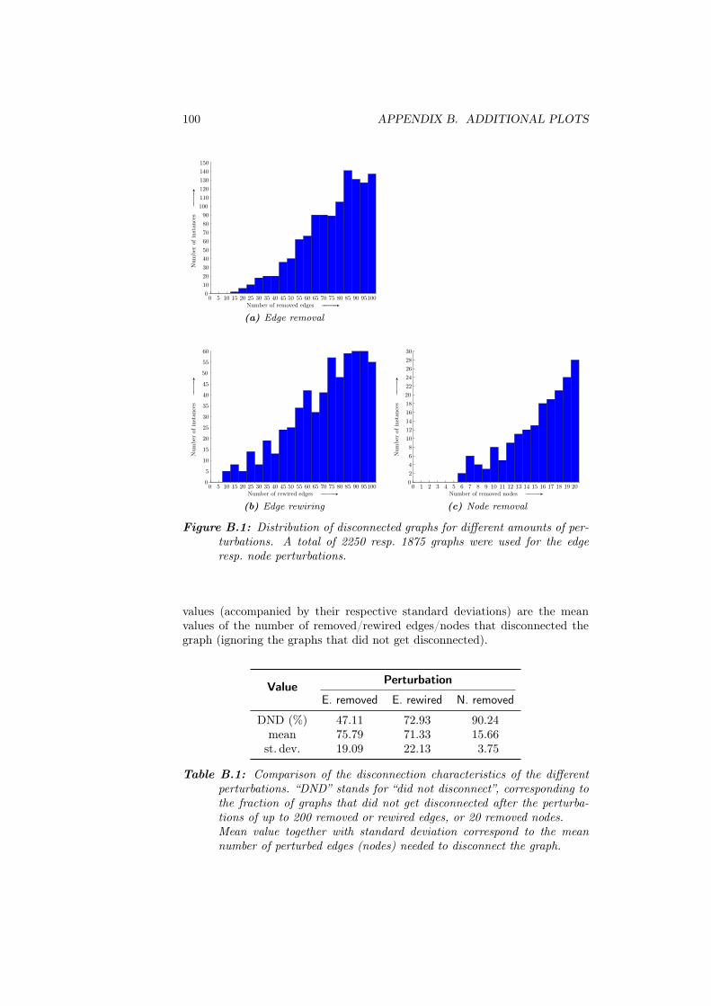
100 APPENDIX B. ADDITIONAL PLOTS
Number of removed edges GGGGGGA
Num
ber
ofin
stan
ces
GGGGGGA
0 5 10 15 20 25 30 35 40 45 50 55 60 65 70 75 80 85 90 951000
10
20
30
40
50
60
70
80
90
100
110
120
130140
150
(a) Edge removal
Number of rewired edges GGGGGGA
Num
ber
ofin
stan
ces
GGGGGGA
0 5 10 15 20 25 30 35 40 45 50 55 60 65 70 75 80 85 90 951000
5
10
15
20
25
30
35
40
45
50
55
60
(b) Edge rewiring
Number of removed nodes GGGGGGA
Num
ber
ofin
stan
ces
GGGGGGA
0 1 2 3 4 5 6 7 8 9 10 11 12 13 14 15 16 17 18 19 200
2
4
6
8
10
12
14
16
18
20
22
24
2628
30
(c) Node removal
Figure B.1: Distribution of disconnected graphs for different amounts of per-turbations. A total of 2250 resp. 1875 graphs were used for the edgeresp. node perturbations.
values (accompanied by their respective standard deviations) are the meanvalues of the number of removed/rewired edges/nodes that disconnected thegraph (ignoring the graphs that did not get disconnected).
ValuePerturbation
E. removed E. rewired N. removed
DND (%) 47.11 72.93 90.24mean 75.79 71.33 15.66
st. dev. 19.09 22.13 3.75
Table B.1: Comparison of the disconnection characteristics of the differentperturbations. “DND” stands for “did not disconnect”, corresponding tothe fraction of graphs that did not get disconnected after the perturba-tions of up to 200 removed or rewired edges, or 20 removed nodes.Mean value together with standard deviation correspond to the meannumber of perturbed edges (nodes) needed to disconnect the graph.
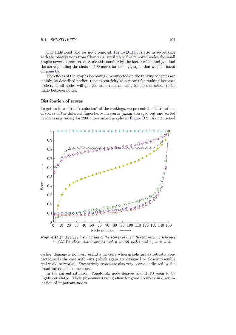
B.1. SENSITIVITY 101
Our additional plot for node removal, Figure B.1(c), is also in accordancewith the observations from Chapter 4: until up to five removed nodes the smallgraphs never disconnected. Scale this number by the factor of 20, and you findthe corresponding threshold of 100 nodes for the big graphs that we mentionedon page 65.
The effects of the graphs becoming disconnected on the ranking schemes aremainly, as described earlier, that excentricity as a means for ranking becomesuseless, as all nodes will get the same rank allowing for no distinction to bemade between nodes.
Distribution of scores
To get an idea of the “resolution” of the rankings, we present the distributionsof scores of the different importance measures (again averaged out and sortedin increasing order) for 200 unperturbed graphs in Figure B.2. As mentioned
Node number GGGGGGA
Scor
eGGGGGGA
0 10 20 30 40 50 60 70 80 90 100 110 120 130 140 1500
0.1
0.2
0.3
0.4
0.5
0.6
0.7
0.8
0.9
1
Figure B.2: Average distribution of the scores of the different ranking schemeson 200 Barabási–Albert graphs with n = 150 nodes and n0 = m = 3 .
earlier, damage is not very useful a measure when graphs are as robustly con-nected as is the case with ours (which again are designed to closely resemblereal world networks). Excentricity scores are also very coarse, indicated by thebroad intervals of same score.
In the current situation, PageRank, node degrees and HITS seem to behighly correlated. Their pronounced rising allow for good accuracy in discrim-ination of important nodes.

102 APPENDIX B. ADDITIONAL PLOTS
B.1.2 Results
Method 1
Most of the curves in Figure B.3 resemble the shape of their counterparts forthe larger graphs (Figure 4.3 on page 67), more precisely the sections of up to1000 perturbed edges.
From about 25 removed edges onward, damage’s sensitivity seems to in-crease linearly with a much steeper slope than that of HITS, PageRank, statusand centroid value. In case of edge addition, it does not deviate at all, as allnodes have and keep the same score.
PageRank and node degrees are only outperformed once, that is by excen-tricity in the case of edge addition. This must not be taken too seriously inlight of the coarseness of excentricity induced rankings.
Number of removed edges GGGGGGA
Dev
iati
onGGGGGGA
0 10 20 30 40 50 60 70 80 90 1000
5
10
15
20
25
30
35
40
45
50
(a) Edge removal
Number of added edges GGGGGGA
Dev
iati
onGGGGGGA
0 10 20 30 40 50 60 70 80 90 1000
0.5
1
1.5
2
2.5
3
3.5
4
(b) Edge addition
Number of rewired edges GGGGGGA
Dev
iati
onGGGGGGA
0 10 20 30 40 50 60 70 80 90 1000
5
10
15
20
25
(c) Edge rewiring
Figure B.3: Sensitivity for deviation measure 1.
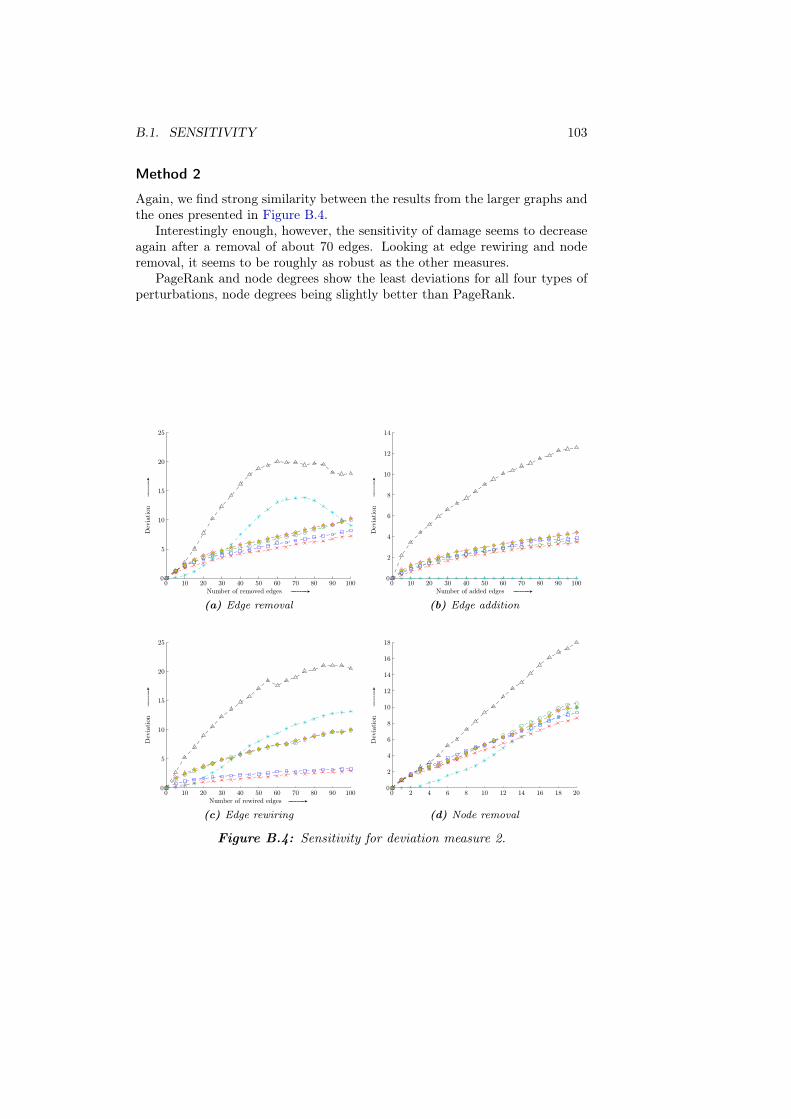
B.1. SENSITIVITY 103
Method 2
Again, we find strong similarity between the results from the larger graphs andthe ones presented in Figure B.4.
Interestingly enough, however, the sensitivity of damage seems to decreaseagain after a removal of about 70 edges. Looking at edge rewiring and noderemoval, it seems to be roughly as robust as the other measures.
PageRank and node degrees show the least deviations for all four types ofperturbations, node degrees being slightly better than PageRank.
Number of removed edges GGGGGGA
Dev
iati
onGGGGGGA
0 10 20 30 40 50 60 70 80 90 1000
5
10
15
20
25
(a) Edge removal
Number of added edges GGGGGGA
Dev
iati
onGGGGGGA
0 10 20 30 40 50 60 70 80 90 1000
2
4
6
8
10
12
14
(b) Edge addition
Number of rewired edges GGGGGGA
Dev
iati
onGGGGGGA
0 10 20 30 40 50 60 70 80 90 1000
5
10
15
20
25
(c) Edge rewiring
Dev
iati
onGGGGGGA
0 2 4 6 8 10 12 14 16 18 200
2
4
6
8
10
12
14
16
18
(d) Node removal
Figure B.4: Sensitivity for deviation measure 2.
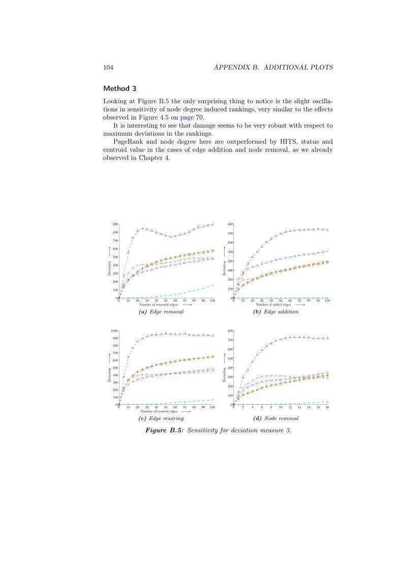
104 APPENDIX B. ADDITIONAL PLOTS
Method 3
Looking at Figure B.5 the only surprising thing to notice is the slight oscilla-tions in sensitivity of node degree induced rankings, very similar to the effectsobserved in Figure 4.5 on page 70.
It is interesting to see that damage seems to be very robust with respect tomaximum deviations in the rankings.
PageRank and node degree here are outperformed by HITS, status andcentroid value in the cases of edge addition and node removal, as we alreadyobserved in Chapter 4.
Number of removed edges GGGGGGA
Dev
iati
onGGGGGGA
0 10 20 30 40 50 60 70 80 90 1000
100
200
300
400
500
600
700
800
900
(a) Edge removal
Number of added edges GGGGGGA
Dev
iati
onGGGGGGA
0 10 20 30 40 50 60 70 80 90 1000
100
200
300
400
500
600
700
800
(b) Edge addition
Number of rewired edges GGGGGGA
Dev
iati
onGGGGGGA
0 10 20 30 40 50 60 70 80 90 1000
100
200
300
400
500
600
700
800
900
1000
(c) Edge rewiring
Dev
iati
onGGGGGGA
0 2 4 6 8 10 12 14 16 18 200
100
200
300
400
500
600
700
800
(d) Node removal
Figure B.5: Sensitivity for deviation measure 3.
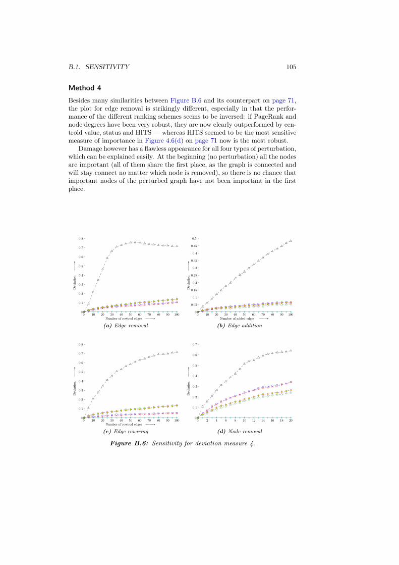
B.1. SENSITIVITY 105
Method 4
Besides many similarities between Figure B.6 and its counterpart on page 71,the plot for edge removal is strikingly different, especially in that the perfor-mance of the different ranking schemes seems to be inversed: if PageRank andnode degrees have been very robust, they are now clearly outperformed by cen-troid value, status and HITS — whereas HITS seemed to be the most sensitivemeasure of importance in Figure 4.6(d) on page 71 now is the most robust.
Damage however has a flawless appearance for all four types of perturbation,which can be explained easily. At the beginning (no perturbation) all the nodesare important (all of them share the first place, as the graph is connected andwill stay connect no matter which node is removed), so there is no chance thatimportant nodes of the perturbed graph have not been important in the firstplace.
Number of rewired edges GGGGGGA
Dev
iati
onGGGGGGA
0 10 20 30 40 50 60 70 80 90 1000
0.1
0.2
0.3
0.4
0.5
0.6
0.7
0.8
(a) Edge removal
Number of added edges GGGGGGA
Dev
iati
onGGGGGGA
0 10 20 30 40 50 60 70 80 90 1000
0.05
0.1
0.15
0.2
0.25
0.3
0.35
0.4
0.45
0.5
(b) Edge addition
Number of rewired edges GGGGGGA
Dev
iati
onGGGGGGA
0 10 20 30 40 50 60 70 80 90 1000
0.1
0.2
0.3
0.4
0.5
0.6
0.7
0.8
(c) Edge rewiring
Dev
iati
onGGGGGGA
0 2 4 6 8 10 12 14 16 18 200
0.1
0.2
0.3
0.4
0.5
0.6
0.7
(d) Node removal
Figure B.6: Sensitivity for deviation measure 4.
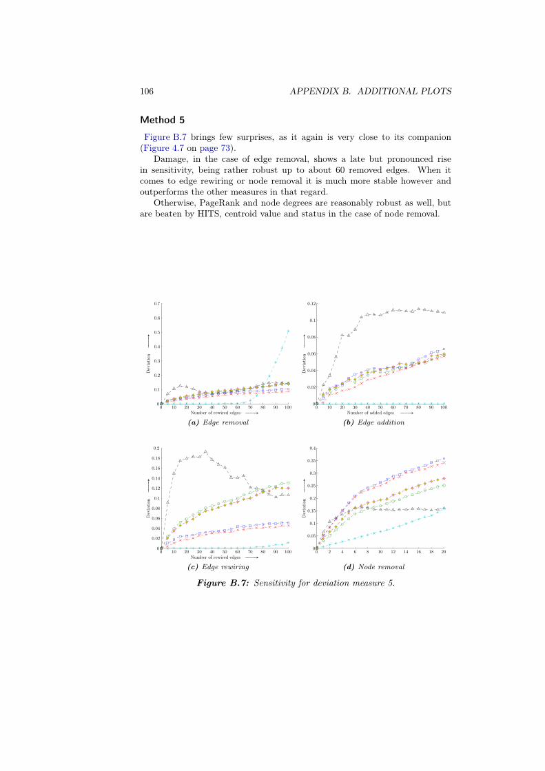
106 APPENDIX B. ADDITIONAL PLOTS
Method 5
Figure B.7 brings few surprises, as it again is very close to its companion(Figure 4.7 on page 73).
Damage, in the case of edge removal, shows a late but pronounced risein sensitivity, being rather robust up to about 60 removed edges. When itcomes to edge rewiring or node removal it is much more stable however andoutperforms the other measures in that regard.
Otherwise, PageRank and node degrees are reasonably robust as well, butare beaten by HITS, centroid value and status in the case of node removal.
Number of rewired edges GGGGGGA
Dev
iati
onGGGGGGA
0 10 20 30 40 50 60 70 80 90 1000
0.1
0.2
0.3
0.4
0.5
0.6
0.7
(a) Edge removal
Number of added edges GGGGGGA
Dev
iati
onGGGGGGA
0 10 20 30 40 50 60 70 80 90 1000
0.02
0.04
0.06
0.08
0.1
0.12
(b) Edge addition
Number of rewired edges GGGGGGA
Dev
iati
onGGGGGGA
0 10 20 30 40 50 60 70 80 90 1000
0.02
0.04
0.06
0.08
0.1
0.12
0.14
0.16
0.18
0.2
(c) Edge rewiring
Dev
iati
onGGGGGGA
0 2 4 6 8 10 12 14 16 18 200
0.05
0.1
0.15
0.2
0.25
0.3
0.35
0.4
(d) Node removal
Figure B.7: Sensitivity for deviation measure 5.
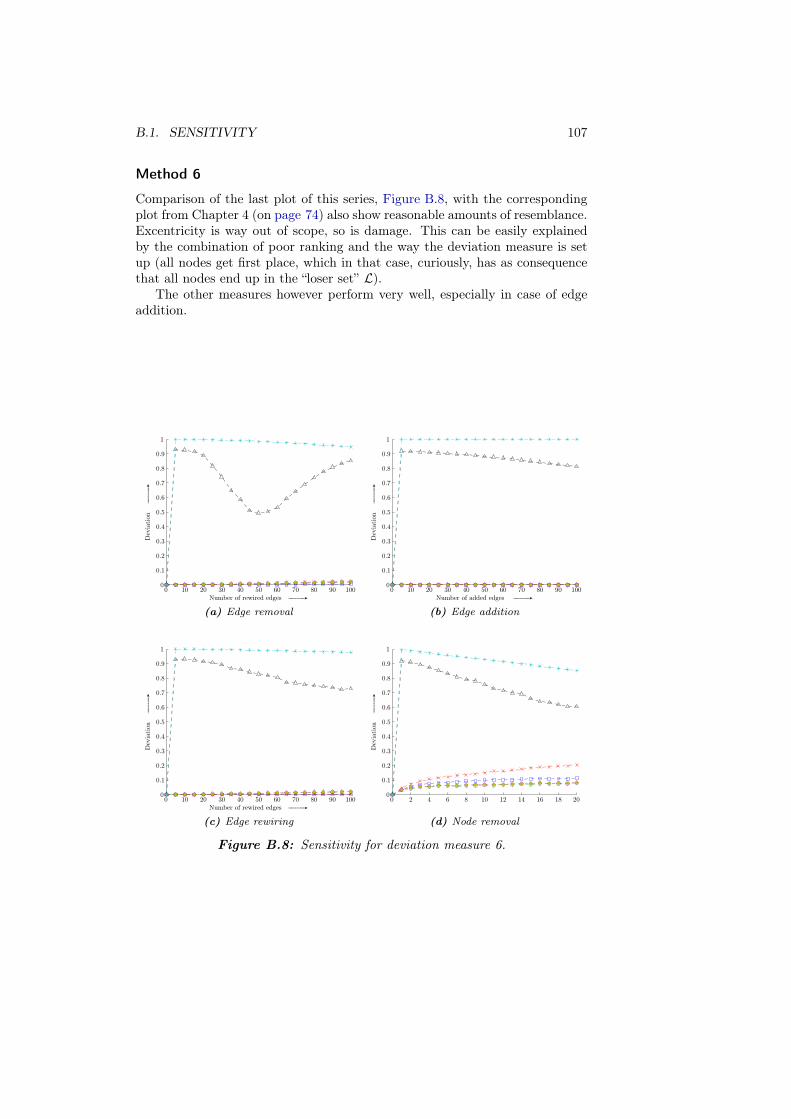
B.1. SENSITIVITY 107
Method 6
Comparison of the last plot of this series, Figure B.8, with the correspondingplot from Chapter 4 (on page 74) also show reasonable amounts of resemblance.Excentricity is way out of scope, so is damage. This can be easily explainedby the combination of poor ranking and the way the deviation measure is setup (all nodes get first place, which in that case, curiously, has as consequencethat all nodes end up in the “loser set” L).
The other measures however perform very well, especially in case of edgeaddition.
Number of rewired edges GGGGGGA
Dev
iati
onGGGGGGA
0 10 20 30 40 50 60 70 80 90 1000
0.1
0.2
0.3
0.4
0.5
0.6
0.7
0.8
0.9
1
(a) Edge removal
Number of added edges GGGGGGA
Dev
iati
onGGGGGGA
0 10 20 30 40 50 60 70 80 90 1000
0.1
0.2
0.3
0.4
0.5
0.6
0.7
0.8
0.9
1
(b) Edge addition
Number of rewired edges GGGGGGA
Dev
iati
onGGGGGGA
0 10 20 30 40 50 60 70 80 90 1000
0.1
0.2
0.3
0.4
0.5
0.6
0.7
0.8
0.9
1
(c) Edge rewiring
Dev
iati
onGGGGGGA
0 2 4 6 8 10 12 14 16 18 200
0.1
0.2
0.3
0.4
0.5
0.6
0.7
0.8
0.9
1
(d) Node removal
Figure B.8: Sensitivity for deviation measure 6.

108 APPENDIX B. ADDITIONAL PLOTS
B.1.3 Conclusions
We have seen that the plots from this series of simulation resemble quite closelyto their bigger counterparts from the 20 times larger networks.
Here as well, PageRank and node degree induced rankings show most of thetime the least sensitivity to perturbations, being challenged however by HITS,centroid value and status in some cases of edge addition or node removal.
The curves for excentricity should not be given too much weight, as, again,on the one hand the induced ranking is extremely coarse and on the other theimpact of disconnection of the graph is significant.

List of Symbols
General notations
n Scalars; lowercase letters1
x Vectors; lowercase bold letters (always supposed to be column vectors,if not transposed), or elementwise in parentheses:
(
x1 x2 . . . xn
)T
M Matrices; uppercase bold letters, or elementwise in brackets:[
m11 m12
m21 m22
]
mij Element (i, j) of Matrix M ; lowercase letters with indices
mrij Element (i, j) of matrix M r (as opposed to (mij)
r)
S Sets; uppercase “calligraphic” letters
Sr r times the Cartesian product of S, i. e. S ×S × . . .×S exactly r times
|S| Cardinality of set S
G Graphs; uppercase “script” letters
P Properties, assumptions; uppercase “Fraktur” letters
≻ M ≻ 0 denotes that M is strictly positive, i. e. mij > 0 for all i, j
� M � 0 denotes that M is strictly non–negative, i. e. mij ≥ 0 for alli, j and for at least one element mij > 0 (so M 6= 0)
〈·〉 Usually denotes an average value
· Within matrices stands for a zero entry (for better legibility)
Specific notations
1n The n–element column vector with all ones, p. 6
1n×n The n× n matrix with all ones, p. 47
AG or just A is usually the adjacency matrix of a graph, p. 4
Cnk Binomial coefficient, Ck
n =(
nk
)
= n!k!(n−k)! for n ≥ k ≥ 0
1 however, v usually denotes some vertex of a graph
109
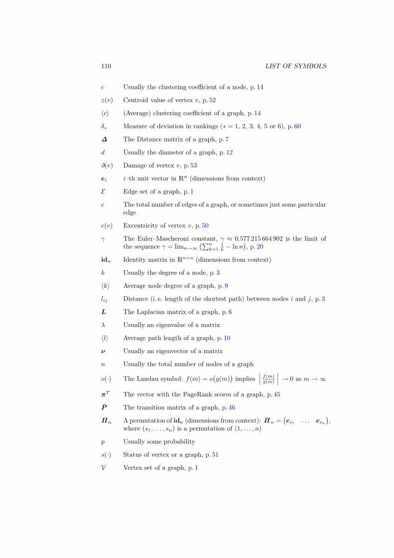
110 LIST OF SYMBOLS
c Usually the clustering coefficient of a node, p. 14
z(v) Centroid value of vertex v, p. 52
〈c〉 (Average) clustering coefficient of a graph, p. 14
δ∗ Measure of deviation in rankings (∗ = 1, 2, 3, 4, 5 or 6), p. 60
∆ The Distance matrix of a graph, p. 7
d Usually the diameter of a graph, p. 12
ð(v) Damage of vertex v, p. 53
ei i–th unit vector in Rn (dimensions from context)
E Edge set of a graph, p. 1
e The total number of edges of a graph, or sometimes just some particularedge
e(v) Excentricity of vertex v, p. 50
γ The Euler–Mascheroni constant, γ ≈ 0.577 215 664 902 is the limit ofthe sequence γ = limn→∞
(∑n
k=11k − lnn
)
, p. 20
idn Identity matrix in Rn×n (dimensions from context)
k Usually the degree of a node, p. 3
〈k〉 Average node degree of a graph, p. 9
lij Distance (i. e. length of the shortest path) between nodes i and j, p. 3
L The Laplacian matrix of a graph, p. 6
λ Usually an eigenvalue of a matrix
〈l〉 Average path length of a graph, p. 10
ν Usually an eigenvector of a matrix
n Usually the total number of nodes of a graph
o(·) The Landau symbol: f(m) = o(
g(m))
implies
f(m)g(m)
→ 0 as m→∞
πT The vector with the PageRank scores of a graph, p. 45
P The transition matrix of a graph, p. 46
Π n A permutation of idn (dimensions from context): Π n =(
es1. . . esn
)
,where (s1, . . . , sn) is a permutation of (1, . . . , n)
p Usually some probability
s(·) Status of vertex or a graph, p. 51
V Vertex set of a graph, p. 1

Bibliography
We tried to provide as many publicly accessible web links as possible.1
[1] William Aiello, Fan R. K. Chung, and Linyuan Lu. A random graph modelfor massive graphs. In STOC ’00: Proceedings of the 32nd Annual ACMSymposium on Theory of Computing, pages 171–180, New York, NY, USA,May 2000. ACM Press. http://www.math.sc.edu/~lu/papers/random.pdf
[2] Réka Z. Albert and Albert-László Barabási. Statistical mechanics of com-plex networks. Reviews of Modern Physics, 74(1):47–96, January 2002.
arXiv:cond-mat/0106096
[3] Luís A. Numes Amaral, Antonio Scala, Marc Barthélémy, and H. EugeneStanley. Classes of small–world networks. Proceedings of the NationalAcademy of Sciences, 97(21):11149–11152, October 2000.
arXiv:cond-mat/0001458
[4] Albert-László Barabási and Réka Z. Albert. Emergence of scaling in ran-dom networks. Science, 286(5439):509–512, October 1999.
arXiv:cond-mat/9910332
[5] Albert-László Barabási, Hawoong Jeong, Zoltan Néda András Schubert,and Tamés Vicsek. Evolution of the social network of scientific collabora-tions. Physica A, 311(3–4):590–614, August 2002. arXiv:cond-mat/0104162
[6] Alain Barrat and Martin Weigt. On the properties of small–world networkmodels. European Physical Journal B, 13(3):547–560, January 2000.
arXiv:cond-mat/9903411
[7] Vladimir Batagelj and Andrej Mrvar. Networks / Pajek, Program forLarge Network Analysis, September 2005.
http://vlado.fmf.uni-lj.si/pub/networks/pajek/
[8] Richard Bellman. On a routing problem. Quarterly of Applied Mathemat-ics, 16(1):87–90, 1958.
1 References of the form arXiv:xxxxxxxx/yyyyyyy can be retrieved directly from the arXiv.orge–Print archive via http://arxiv.org/abs/xxxxxxxx/?yyyyyyy or one of its mirrors.
111
112 BIBLIOGRAPHY
[9] Norman L. Biggs. Algebraic graph theory, volume 67 of Cambridge Tractsin Mathematics. Cambridge University Press, London, New York, 1974.
[10] Béla Bollobás. Degree sequences of random graphs. Discrete Mathematics,33(1):1–19, January 1981. http://dx.doi.org/10.1016/0012-365X(81)90253-3
[11] Béla Bollobás. Random Graphs. Academic Press, London, UK, 1985.
[12] Béla Bollobás and Oliver Riordan. The diameter of a scale–free randomgraph. Combinatorica, 24(1):5–34, January 2004.
http://www.math.cornell.edu/~durrett/math777/diamSF.pdf
[13] Sergey Brin and Lawrence Page. The anatomy of a large–s1cale hyper-textual web search engine. Computer Networks and ISDN Systems, 30(1–7):107–117, April 1998. http://www-db.stanford.edu/pub/papers/google.pdf
[14] Andrei Z. Broder, Ravi Kumar, Farzin Maghoul, Prabhakar Raghavan,Sridhar Rajagopalan, Raymie Stata, Andrew Tomkins, and Janet L.Wiener. Graph structure in the web. Computer Networks, 33(1–6):309–320, 2000. http://www9.org/w9cdrom/160/160.html
[15] Fan Chung and Linyuan Lu. The diameter of sparse random graphs.Advances in Applied Mathematics, 26(4):257–279, May 2001.
http://www.math.ucsd.edu/~fan/dia.pdf
[16] Reuven Cohen and Shlomo Havlin. Scale–free networks are ultrasmall.Physical Review Letters, 90(5):058701/1–4, February 2003.
arXiv:cond-mat/0205476
[17] Edsger W. Dijkstra. A note on two problems in connexion with graphs.Numerische Mathematik, 1:269–271, 1959.
http://dz-srv1.sub.uni-goettingen.de/sub/digbib/loader?did=D196313
[18] Roger C. Entringer, Douglas E. Jackson, and David A. Snyder. Distancein graphs. Czechoslovak Mathematical Journal, 26(2):283–296, June 1976.
[19] Paul Erdös and Alfréd Réyni. On random graphs. Publicationes Mathe-maticae, 6:290–297, 1959.
[20] Ayman Farahat, Thomas Lofaroa, Joel C. Miller, Gregory Rae, and Les-ley A. Ward. Existence and uniqueness of ranking vectors for linear linkanalysis. SIAM Journal on Scientific Computing, 2004. Submitted April2004.
[21] Miroslav Fiedler. Algebraic connectivity of graphs. Czechoslovak Mathe-matical Journal, 23(98):298–305, 1973.
113
[22] Agata Fronczak, Piotr Fronczak, and Janusz A. Hołyst. Mean–field theoryfor clustering coefficients in Barabási–Albert networks. Physical Revue E,68(4):046126/1–4, October 2003. arXiv:cond-mat/0306255
[23] Agata Fronczak, Piotr Fronczak, and Janusz A. Hołyst. Average pathlength in random networks. Physical Revue E, 70(5):056110/1–7, Novem-ber 2004. arXiv:cond-mat/0212230
[24] Gene H. Golub and Charles F. Van Loan. Matrix Computations. JohnsHopkins University Press, Baltimore, MD, USA, 2nd edition, 1989.
[25] Google Inc. The Google timeline, December 2004.http://www.google.com/intl/en/corporate/timeline.html
[26] Ramesh Govindan and Hongsuda Tangmunarunkit. Heuristics for internetmap discovery. In IEEE INFOCOM 2000, volume 3, pages 1371–1380, TelAviv, Israel, March 2000. IEEE.
http://www.isi.edu/div7/publication_files/heuristics.pdf
[27] Geoffrey Grimmett. Percolation. Springer, Berlin, Germany, 2nd edition,1999.
[28] Frank Harary. Status and contrastatus. Sociometry, 22(1):23–43, March1959. http://links.jstor.org/sici?sici=0038-0431(195903)22:1<23:SAC>
[29] Frank Harary and Robert Z. Norman. The dissimilarity characteristic ofhusimi trees. The Annals of Mathematics, 58(1):134–141, July 1953.
http://links.jstor.org/sici?sici=0003-486X(195307)2:58:1<134:TDCOHT>
[30] Taher H. Haveliwala and Sepandar D. Kamvar. The second eigenvalue ofthe google matrix. Technical Report 2003-20, Stanford University, Depart-ment of Computer Science, March 2003. http://dbpubs.stanford.edu/pub/2003-20/
[31] Roger A. Horn and Charles R. Johnson. Matrix Analysis. CambridgeUniversity Press, Cambridge, UK, 1985.
[32] Takashi Ito, Kosuke Tashiro, Shigeru Muta, Ritsuko Ozawa, TomokoChiba, Mayumi Nishizawa, Kiyoshi Yamamoto, Satoru Kuhara, andYoshiyuki Sakaki. Toward a protein-protein interaction map of the bud-ding yeast: A comprehensive system to examine two-hybrid interactionsin all possible combinations between the yeast proteins. Proc. of the Nat.Academy of Sciences of the USA, 97:1143–1147, February 2000.
http://biology.uark.edu/ipinto/biol5334/17.pdf
[33] Camille Jordan. Sur les assemblages de lignes. Journal für die reine undangewandte Mathematik, 70:185–190, 1869.
114 BIBLIOGRAPHY
[34] Lester R. Ford Jr. Network flow theory. Paper P–923, The RAND Cor-peration, Santa Moncia, CA, USA, August 1956.
[35] Jon M. Kleinberg. Authoritative sources in a hyperlinked environment.Journal of the ACM, 46(5):604–632, 1999.
http://www.cs.cornell.edu/home/kleinber/auth.pdf
[36] Florian Knorn. Supplementary material to this Studienarbeit, September2005. http://www.florian-knorn.com/index.php?nav=work&cat=stud
[37] Amy N. Langville and Carl D. Meyer. Deeper inside PageRank. InternetMathematics, 1(3):335–380, 2004.
http://www.internetmathematics.org/volumes/1/3/Langville.pdf
[38] Amy N. Langville and Carl D. Meyer. A survey of eigenvector methodsof web information retrieval. SIAM Review, 47(1):135–161, March 2005.
http://meyer.math.ncsu.edu/Meyer/PS_Files/Survey.pdf
[39] Ney Lemke, Fabiana Herédita, Cláudia K. Barcellos, Adriana N. dos Reis,and José C. M. Mombach. Essentiality and damage in metabolic networks.Bioinformatics, 20(1):115–119, January 2004.
http://www.inf.unisinos.br/~mombach/Ecoli.pdf
[40] Bo Lewin, editor. Sex i Sverige. Om sexuallivet i Sverige 1996 [Sex inSweden. About Sex habits in Sweden in 1996]. Statens Folkhälsoinstitut[Swedish National Institute of Public Health], Stockholm, Sweden, 1998.
[41] Fredrik Liljeros, Christofer R. Edling, Luís A. Nunes Amaral, H. EugeneStanley, and Yvonne Åberg. The web of human sexual contacts. Nature,411(6840):907–908, 2001. arXiv:cond-mat/0106507
[42] David G. Luenberger. Introduction to Dynamic Systems. Theory, Models& Applications. John Wiley & Sons, New York, NY, USA, 1979.
[43] Carl D. Meyer. Matrix analysis and applied linear algebra. SIAM, Philadel-phia, PA, USA, 2000.
[44] Stanley Milgram. The small world problem. Psychology Today, 1(2):60–67, May 1967.
[45] Joel C. Miller, Gregory Rae, Fred Schaefer, Lesley A. Ward, Thomas Lo-Faro, and Ayman Farahat. Modifications of Kleinberg’s HITS algorithmusing matrix exponentiation and web log records. In SIGIR ’01: Proceed-ings of the 24th annual international ACM SIGIR conference on Researchand development in information retrieval, pages 444–445, New York, NY,USA, 2001. ACM Press. http://www.damtp.cam.ac.uk/user/jcm52/pubs/sigir.pdf
115
[46] Bohan Mohar. Isoperimetric numbers of graphs. Journal of CombinatorialTheory Series B, 47(3):274–291, December 1989.
http://dx.doi.org/10.1016/0095-8956(89)90029-4
[47] Bohan Mohar. Combinatorics, and Applications, volume 2, pages 871–898.John Wiley and Sons, New York, NY, USA, 1991. Y. Alavi, G. Chartrand,O. R. Ollerman and A. J. Schwenk (ed.).
[48] Cleve Moler. The world’s largest matrix computation. Matlab News andNotes, October 2002.
http://www.mathworks.com/company/newsletters/news_notes/clevescorner/oct02_cleve.html
[49] Mark E. J. Newman, Cris Moore, and Duncan J. Watts. Mean–fieldsolution of the small–world network model. Physical Review Letters,84(14):3201–3204, April 2000. arXiv:cond-mat/9909165
[50] Mark E. J. Newman, Steven H. Strogatz, and Duncan J. Watts. Randomgraphs with arbitrary degree distributions and their applications. PhysicalRevue E, 64(2):026118/1–17, August 2001. arXiv:cond-mat/0007235
[51] Andrew Y. Ng, Alice X. Zheng, and Micheal I. Jordan. Link analysis,eigenvectors and stability. In IJCAI ’01: Proceedings of the 17th Interna-tional Joint Conference on Artificial Intelligence, pages 903–910, August2001. http://www.cs.berkeley.edu/~ang/papers/ijcai01-linkanalysis.pdf
[52] Lawrence Page, Sergey Brin, Rajeev Motwani, and Terry Winograd. ThePageRank citation ranking: Bringing order to the web. Technical Report1999-66, Stanford University, Department of Computer Science, November1999. http://dbpubs.stanford.edu/pub/1999-66/
[53] Francesco Rao and Amedeo Caflisch. The protein folding network. Journalof Molecular Biology, 342(1):299–306, September 2004.
arXiv:q-bio.BM/0403034
[54] Sidney Redner. How popular is your paper? An empirical study of thecitation distribution. European Physical Journal B, 4(2):131–134, July1998. arXiv:cond-mat/9804163
[55] Antonio Scala, Luís A. Numes Amaral, and Marc Barthélémy. Small–world networks and the conformation space of a short lattice polymerchain. Europhysics Letters, 55(4):594–600, August 2001.
arXiv:cond-mat/0004380
[56] Jean Schmith, Ney Lemke, José C.M. Mombach, Patrícia Benelli, Cláu-dia K. Barcellos, and Guilherme B. Bedin. Damage, connectivity andessentiality in protein–protein interaction networks. Physica A, 349(3–
116 BIBLIOGRAPHY
4):675–684, April 2005. http://www.inf.unisinos.br/~mombach/protnetv2.pdf
[57] Peter J. Slater. Maximum facility location. Journal of Research of theNational Bureau of Standards B, 79:107–115, 1975.
[58] Daniel A. Spielman. Spectral graph theory and its applications. Lecturenotes, September 2004. http://www-math.mit.edu/~spielman/eigs/
[59] Peter Uetz and Loic Giot. A comprehensive analysis of protein–proteininteractions in saccharomyces cerevisiae. Nature, 403:623–627, February2000. http://www.nature.com/nature/journal/v403/n6770/full/403623a0_fs.html
[60] Alexei Vázquez, Romualdo Pastor–Satorras, and Alessandro Vespignani.Internet topology at the router and autonomous system level. arXive–Print, June 2002. arXiv:cond-mat/0206084
[61] Michele Vendruscolo, Nikolay V. Dokholyan, Emanuele Paci, and MartinKarplus. Small–world view of the amino acids that play a key role inprotein folding. Physical Revue E, 65(6):061910/1–4, June 2002.
http://dokhlab.unc.edu/papers/vdpk_pre02.pdf
[62] Duncan J. Watts and Steven H. Strogatz. Collective dynamics of ‘small–world’ networks. Nature, 393(6684):440–442, June 1998.
http://tam.cornell.edu/SS_nature_smallworld.pdf
[63] Stefan Wuchty and Peter F. Stadler. Centers of complex networks. Journalof Theoretical Biology, 223(1):45–53, July 2003.
http://www.nd.edu/~swuchty/Download/center.pdf
[64] Haiyuan Yu, Dov Greenbaum, Hao X. Lu, Xiaowei Zhu, and Mark Ger-stein. Genomic analysis of essentiality within protein networks. Trends inGenetics, 20(6):227–231, June 2004.
http://papers.gersteinlab.org/e-print/essen/reprint.pdf
[65] Haiyuan Yu, Dov Greenbaum, Hao X. Lu, Xiaowei Zhu, and Mark Ger-stein. Supplementary material to [64], February 2004.
http://bioinfo.mbb.yale.edu/network/essen/Sup.pdf