Ravello Lectures on Geometric Calculus – Part I - arXiv · arXiv:math-ph/0501001v2 3 Jan 2005 Ravello Lectures on Geometric Calculus – Part I Jenny Harrison Department of Mathematics

arX

iv:m

ath-

ph/0

5010

01v2

3 J

an 2

005

Ravello Lectures on Geometric

Calculus – Part I

Jenny Harrison

Department of Mathematics

University of California, Berkeley

December 31, 2004

E-mail address : [email protected]

http://arXiv.org/abs/math-ph/0501001v2

Preface

In these notes we present a new approach to calculus in which moreefficient choices of limits are taken at key points of the development.For example, k-dimensional tangent spaces are replaced by represen-tations of simple k-vectors supported in a point as limits of simplicialk-chains in a Banach space (much like Dirac monopoles). This sub-tle difference has powerful advantages that will be explored. Throughthese “infinitesimals”, we obtain a coordinate free theory on manifoldsthat builds upon the Cartan exterior calculus. An infinite array of ap-proximating theories to the calculus of Newton and Lebiniz becomesavailable and we can now revisit old philosophical questions such aswhich models are most natural for the continuum or for physics.

Within this new theory of Geometric Calculus are found the clas-sical theory on smooth manifolds, as well as three distinct, new exten-sions. All three can be seen as part of the space of polyhedral chainscompleted with respect to what the author calls the “natural norm”.The author calls elements of the Banach space obtained upon comple-tion “chainlets”.

We take many viewpoints in mathematics and its applications, beit smooth manifolds, Lipschitz structures, polyhedra, fractals, finiteelements, soap films, measures, numerical methods, etc. The choice setsthe stage and determines our audience and our methods. No particularviewpoint is “right” for all applications. The Banach space of chainletsunifies these viewpoints.

(1) Discrete Calculus∗ with convergence to the smooth contin-nuum, including more general theorems of Stokes, Green andGauss.

(2) Bilayer Calculus with applications to the calculus of varia-tions including Plateau’s problem (soap bubbles).

(3) Calculus on Fractals

∗Some aspects of this are contained in the paper [10] and slides prepared for theCaltech meeting in October, 2003 on Discrete Geometry for Mechanics are availableon line at http://math.berkeley.edu/∼harrison.

3

http://math.berkeley.edu/~harrison

4 PREFACE

The discrete theory is perhaps the most far reaching. Poincaretaught us to use a simplicial complex as the basic discrete model. Ithas become fashionable to use Whitney forms [2] as cochains and theyare based on the simplicial complex. However, there is a great dealinformation within a simplicial complex that is not needed for calculus.There are corners, matching boundaries of simplices, ratios of lengthto area, and so forth. The standard proof to Stokes’ theorem relies onboundaries matching and cancelling with opposite orientation wherethey meet. However, problems of approximation sometimes arise in thecontinuum limit, as a finer and finer mesh size is used. For example,

• Supposed approximations may not converge• Vectors, especially normal vectors, may be hard to define• Cochains fail to satisfy a basic property such as commutativity

or associativity of wedge product, or existence of Hodge star.

One may discard much of the information in a simplicial com-plex and instead use sums of what are essentially “weighted orientedmonopoles and higher order dipoles” as approximators for both do-mains and integrands. (These will be fully described in the lectures.)Standard operators such as boundary, coboundary, exterior derivativeand Laplace are naturally defined on these “element chains”. Integralrelations of calculus are valid and essentially trivial at this discrete leveland converge to the continuum limit. Vectors have discrete counter-parts, including normal vectors, and discrete cochains are well behaved.

One of our goals in these notes is to write the theorems of Stokes,Gauss and Green in such a concise and clear manner that all mannerof domains are permitted without further effort. We obtain this byfirst treating the integral as a bilinear functional on pairs of integrandsand domains, i.e., forms and chainlets. Secondly, we define a geometricHodge star operator ⋆ on domains A and proving for k-forms ω inn-space

∫

∂A

ω =

∫

A

dω

and ∫

⋆A

⋆ω =

∫

A

ω

with appropriate assumptions on the domain and integrand (see Chap-ter 4). One may immediately deduce

∫

⋆∂A

ω = (−1)k(n−k)

∫

A

d ⋆ ω

PREFACE 5

and ∫

∂⋆A

ω = (−1)(k+1)(n−k−1)

∫

A

⋆dω

which are generalized and optimal versions of the divergence and curltheorems, respectively.

Arising from this theory are new, discrete approximations for thereal continuum. Morris Hirsch wrote,† on December 13, 2003.

A basic philosophical problem has been to make sense of“continuum”, as in the space of real numbers, without in-troducing numbers. Weyl [5] wrote, “The introduction ofcoordinates as numbers... is an act of violence”. Poincarewrote about the “physical continuum” of our intuition,as opposed to the mathematical continuum. Whitehead(the philosopher) based our use of real numbers on our in-tuition of time intervals and spatial regions. The Greekstried, but didn’t get very far in doing geometry withoutreal numbers. But no one, least of all the Intuitionists,has come up with even a slightly satisfactory replacementfor basing the continuum on the real number system, orbasing the real numbers on Dedekind cuts, completion ofthe rationals, or some equivalent construction.

Harrison’s theory of chainlets can be viewed as a dif-ferent way to build topology out of numbers. It is amuch more sophisticated way, in that it is (being) de-signed with the knowledge of what we have found tobe geometrically useful (Hodge star, Stokes’ theorem,all of algebraic topology,. . .), whereas the standarddevelopment is just ad hoc– starting from Greek geom-etry, through Newton’s philosophically incoherent calcu-lus, Descarte’s identification of algebra with geometry,with additions of abstract set theory, Cauchy sequences,mathematical logic, categories, topoi, probability theory,and so forth, as needed. We could add quantum mechan-ics, Feynman diagrams and string theory! The point isthis is a very roundabout way of starting from geometry,building all that algebraic machinery, and using it for ge-ometry and physics. I don’t think chainlets, or any otherpurely mathematical theory, will resolve this mess, butit might lead to a huge simplification of important partsof it.

†e-mail message, quoted with permission

6 PREFACE

Readers may choose any number of points of view. Smooth mani-folds, discrete element chains, polyedra, fractals, any dense set of chain-lets will produce the same results in the limit, which links togethernumerous approaches some of which seemed distantly related, at best.Philosophically, we may not know the most natural models for physics,but we provide here various options which all converge to the contin-uum limit and are consistent with each other and standard operators ofmathematics and physics. We anticipate applications to physics, con-tinuum mechanics, biology, electromagnetism, finite element method,PDE’s, dynamics, computation, wavelets, vision modeling as well asto pure mathematics (topology, foundations, geometry, dynamical sys-tems) and give examples in the notes that follow. Indeed, the au-thor proposes that the discrete theory provides a foundation for newmodels for quantum field theory, a topic under development. Alge-braic/geometric features of the models make them especially enticing.It is worse to be oblivious to the importance of a new theory than to beoverly excited, and the author chooses to err on the side of the latter.

I am grateful to the Scientific Council of GNFM for inviting me togive this course, and to the Director of the Ravello Summer School,Professor Salvatore Rionero, for his elegant hospitality. I also wish tothank Antonio Di Carlo, Paolo Podio-Guidugli, Gianfranco Capriz andthe other participants of the Ravello Summer School for their interestin my work and for encouraging me to put my scribbled lecture notesinto their present form. Above all, I thank Morris Hirsch and JamesYorke for listening over these years. Their support and encouragementhave been critical to the success of this research program.

• Harrison, Jenny, Stokes’ theorem on nonsmooth chains, Bul-letin AMS, October 1993.

• –, Continuity of the Integral as a Function of the Domain,Journal of Geometric Analysis, 8 (1998), no. 5, 769–795.

• –.Isomorphisms differential forms and cochains, Journal of Geo-metric Analysis, 8 (1998), no. 5, 797–807.

• –, Geometric realizations of currents and distributions, Pro-ceedings of Fractals and Stochastics III, Friedrichsroda, Ger-man, 2004.

• –,Geometric Hodge star operator with applications to the the-orems of Gauss and Green, to appear, Proc Cam Phil Soc.

• –, Cartan’s Magic Formula and Soap Film structures, Journalof Geometric Analysis

• –, On Plateau’s Problem with a Bound on Energy, Journal ofGeometric Analysis

PREFACE 7

• –, Discrete Exterior Calculus with Convergence to the SmoothContinuum, preprint in preparation

• –, Measure and dimension of chainlet domains, preprint inpreparation

8 PREFACE

Geometric Integration Theory

Geometric Integration Theory (GIT), the great classic of HasslerWhitney [2], was an attempt to articulate the approach to calculusfavored by Leibnitz of approximation of domains by polyhedral chainsrather than by parametrization by locally smooth coordinate charts.

Approximation by polyhedral chains defined using finite sums ofcells, simplexes, cubes, etc., has been a technique commonly used byapplied mathematicians, engineers, physicists and computer scientistsbut has not had the benefit of rigorous mathematical support to guar-antee convergence. We often create grids around a domain dependingon a small scale parameter, perform calculations on each grid, let theparameter tend to zero, and hope the answers converge to somethingmeaningful. Sometimes the limit appears to exist, but actually doesnot. An example, given by Schwarz, is that of a cylinder with unitarea, but approximated by simplicial chains with vertices on the cylin-der whose areas limit to any positive number in the extended reals.

Whitney’s theory was based on the idea of completing the space ofpolyhedral chains with a norm and proving continuity of basic operatorsof calculus with respect to that norm, thereby obtaining a theory ofcalculus on all points in the Banach space. This approach had workedwell for spaces of functions and Whitney was the first to try it out fordomains of integration.

Unfortunately, his definitions from the late 1940’s brought withthem serious technical obstructions that precluded extension of mosttheorems of calculus. His first norm, the sharp norm, does not havea continuous boundary operator so one cannot state the generalizedStokes’ theorem ∫

∂A

ω =

∫

A

dω

for elements A of the Banach space obtained upon completion. (It isnot necessary for the reader to know the definition of the sharp normas given by Whitney to understand these notes.)

His second norm, the flat norm, has a continuous boundary oper-ator built into it, but does not have a continuous Hodge star operator,and thus one may not state either a generalized divergence or curl the-orem in the flat normed space. (See Table 1.) In this introduction, weuse terminology such as “flat norm” and “Hodge star operator” thatwill be defined in later sections.

GEOMETRIC CALCULUS 9

Geometric Measure Theory

Geometric measure theory [4], the study of domains through weakconvergence and measures, took the approach of using dual spaces ofdifferential forms and had greater success in extending calculus. Theextension of the Gauss-Green theorem, credited to de Giorgi and Fed-erer, was a striking application of GMT. Their divergence theoremholds for an n-dimensional current C with Ln Lebesgue measurablesupport and Hn−1 Hausdorff measurable current boundary. The vectorfield F is assumed to be Lipschitz. Their conclusion takes the form

∫

∂C

F (x) · n(C, x)dHn−1x =

∫

C

divF (x)dLnx.

The hypotheses imply the existence a.e. of measure theoretic normalsn(C, x) to the (“current”) boundary. See [4]

A second crowning achievement of GMT was a solution to the prob-lem of Plateau. Plateau [1] studied soap films experimentally and no-ticed that soap film surfaces could meet in curves in only two ways:Three films can come together along a curve at equal 120 degree an-gles, and four such curves can meet at a point at equal angles of about109 degrees.

The question arose: Given a closed loop of wire, is there a surfacewith minimal area spanning the curve? Douglas won the first Field’smedal for his solution in the class of smooth images of disks. Federerand Fleming were able to provide a solution within the class of em-bedded, orientable surfaces. They do not model branched surfaces anddo not permit the Moebius strip solution as a possible answer, thoughsuch solutions do occur in nature.

The most recent area of application of GMT has been with fractalsand that has reinervated interest in the theory as it provides rigorousmethods for studying integral and measure of nonsmooth domains. Itis generally accepted that nonsmooth sets appear commonly in math-ematics as well as in the real world. Paths of fractional Brownianmotion have become fashionable as models of everyday phenomenonsuch as stock market models, resulting in a growing demand for resultsof geometric measure theory.

Geometric Calculus

In these lectures will be developed a third approach that the authorcalls “geometric calculus” (GC). The theory of GC begins in Lecture

10 PREFACE

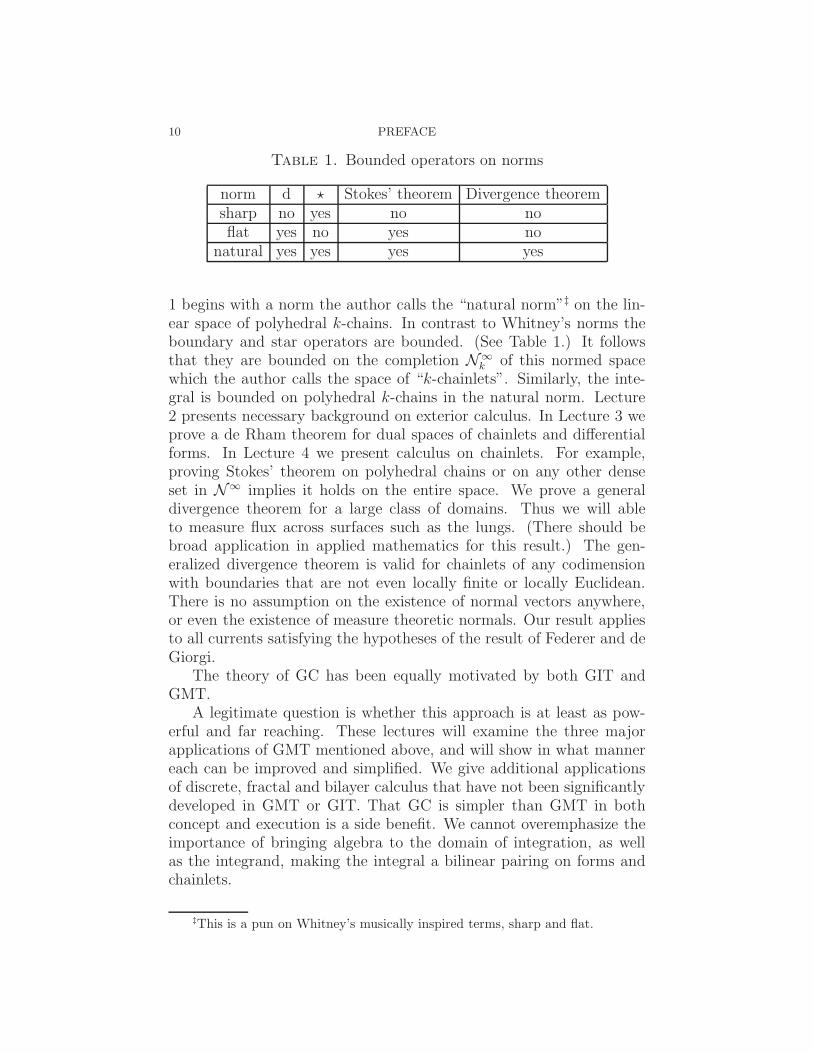
Table 1. Bounded operators on norms

norm d ⋆ Stokes’ theorem Divergence theoremsharp no yes no noflat yes no yes no

natural yes yes yes yes

1 begins with a norm the author calls the “natural norm”‡ on the lin-ear space of polyhedral k-chains. In contrast to Whitney’s norms theboundary and star operators are bounded. (See Table 1.) It followsthat they are bounded on the completion N∞

k of this normed spacewhich the author calls the space of “k-chainlets”. Similarly, the inte-gral is bounded on polyhedral k-chains in the natural norm. Lecture2 presents necessary background on exterior calculus. In Lecture 3 weprove a de Rham theorem for dual spaces of chainlets and differentialforms. In Lecture 4 we present calculus on chainlets. For example,proving Stokes’ theorem on polyhedral chains or on any other denseset in N∞ implies it holds on the entire space. We prove a generaldivergence theorem for a large class of domains. Thus we will ableto measure flux across surfaces such as the lungs. (There should bebroad application in applied mathematics for this result.) The gen-eralized divergence theorem is valid for chainlets of any codimensionwith boundaries that are not even locally finite or locally Euclidean.There is no assumption on the existence of normal vectors anywhere,or even the existence of measure theoretic normals. Our result appliesto all currents satisfying the hypotheses of the result of Federer and deGiorgi.

The theory of GC has been equally motivated by both GIT andGMT.

A legitimate question is whether this approach is at least as pow-erful and far reaching. These lectures will examine the three majorapplications of GMT mentioned above, and will show in what mannereach can be improved and simplified. We give additional applicationsof discrete, fractal and bilayer calculus that have not been significantlydeveloped in GMT or GIT. That GC is simpler than GMT in bothconcept and execution is a side benefit. We cannot overemphasize theimportance of bringing algebra to the domain of integration, as wellas the integrand, making the integral a bilinear pairing on forms andchainlets.

‡This is a pun on Whitney’s musically inspired terms, sharp and flat.


As noted above, any dense subset of chainlets leads to a full theoryof calculus in the limit. However, different choices of subsets maypresent quite different initial results before taking limits in the chainletspace. For example, it is shown in Lecture 5 that smooth differentialforms are dense in the space of chainlets, as are smooth submanifolds.Lecture 6 presents a theory of locally compact abelian groups leadingto a theory of distributions with the notion of differentiaion. Lecture7 introduces a dense subset of newly discovered chainlets consistingof finite sums of what the author calls “k-elements”. Each k-elementis supported in a single point and makes rigorous the notion of an“infinitesimal” of Newton and Leibnitz. We distinguish two meaningsof an “infinitesimal”, although we do not use this term beyond theintroduction. One is an “infinitesimal domain”, the other is its dual,an “infinitesimal form”. A k-element is a kind of infinitesimal domain.

Higher order k-elements of order s are also introduced in Lecture7. A k-element of order zero is the same as a k-element which canbe thought of as a geometric analogue of the Dirac delta point or amonopole. In the natural norm Banach space the distance between twomonopoles at points p and q is proportional to the distance betweenp and q. Contrast this with the theory of distributions where metricsare defined weakly. Each k-element of order s is again supported in apoint. For s = 1 we have a dipole, s = 2, a quadrupole, and so forth.The number s corresponds loosely to an s order derivative of a deltafunction, though of course our elements are delta points, the geometricanalogs of delta functions and are defined in arbitrary dimension andcodimension. There is no upper bound on s, even in dimension one,although k is bounded by the ambient dimension. Each k-element oforder s has a well-defined boundary as a sum of (k−1)-element or order(s + 1) and it has a discrete analog of a normal bundle defined via thegeometric star operator. It is striking that the divergence theorem canbe proved at a single point. The space N∞ extends standard geometricstructures by adding geometric and algebraic attributes to points. Weform our basic “multiorder k-element chains” from the direct sum ofspaces of k-element chains of order s. The direct sum is required forthe boundary and star operators to be closed. Since such “discrete”chains are dense in the space of chainlets, we may develop a discreteapproach to the full calculus. Elements of the dual space to k-elementchains converge to smooth differential forms in the limit. With this weare able to define operators on forms as dual to geometrically definedoperators on k-elements. The forms, which “measure” cells, becomeperfectly matched for their job, in a coordinate free fashion. In the full

12 PREFACE

discrete theory we quantize matter and energy with models that maketheir identification transparent, up to a constant.∗

It is a subtle, but significant difference to begin with k-elementchains (GC) rather than polyhedral chains (GIT) or k-vectors (GMT).With our approach, at the starting point of GC, we reveal a com-mon denominator for forms and chains that is the essence of Poincareduality. We make this precise via an extension of tensor analysis, us-ing what the author calls “multitensors” that are monopoles, dipoles,quadrupoles, etc. It is striking that the subspace of k-element chainsis reflexive, although the space of chainlets is not, neither are othersubspaces such as differential forms or polyhedral chains. In the ap-plication to smooth manifolds, there is no longer reliance on tangentspaces, the hardy tools of mathematics. Instead we use the versatileand rich k-elements which have boundaries defined, where other op-erators apply and the essence of calculus is found. Linear algebra isvalid on k-elements and carries over locally to chainlets, much as it hasdone for manifolds via tangent spaces. The use of k-elements in placeof k-dimensional tangent spaces opens up new vistas well beyond thescope of the integral methods of GIT and that is why we prefer to callit GC. New fields of enquiry emerge which will be highlighted as thelectures develop.

Outline

1. Chainlets2. Exterior algebra3. Differential forms and cochains (de Rham theorem)4. Calculus on fractals – star operator (no assumptions of self

similarity, connectivity, local Euclidean, or locally finite mass.Chainlets are useful for modeling structures in the physicalsciences with nontrivial local structures.)

5. Poincare duality for chains and cochainlets (chainlet repre-sentations of differential forms, cap product, wedge product,convolution product)

6. Locally compact abelian groups7. Discrete calculus (part I) (a coordinate free approach that con-

tains calculus on smooth manifolds, numerical methods, andmore) The first half of this chapter appears in the first part ofthese lecture notes presented below. The second half, as wellas the following chapters, will appear in the second part tofollow.

∗e = mc2


8. Bilayer calculus (soap film structures, calculus of variations onsoap films, Lipid bilayers, immiscible fluids, fractures, multi-layer calculus, bilayer foliations, Frobenius theorem, differen-tial equations)

9. Measure theory (lower semi continuity of s-mass, k-vector val-ued additive set functions, s-normable chainlets)

10. Applications

Because these notes are only meant as an introduction to the theory,a number of important results, of necessity, have been left out.

CHAPTER 1

Chainlets

Polyhedral chains

A cell σ in Rn is the nonempty intersection of finitely many closedaffine half spaces. The dimension of σ is k if k is the dimension ofthe smallest affine subspace E containing σ. The support sptσ of σ isthe set of all points in the intersection of half spaces that determine σ.

Assume k > 0. An orientation of E is an equivalence class ofordered bases for the linear subspace parallel to E where two basesare equivalent if and only if their transformation matrix has positivedeterminant. An orientation of σ is defined to be an orientation ofits subspace E. Henceforth, all k-cells are assumed to be oriented.(No orientation need be assigned to 0-cells which turn out to be singlepoints x in R

n. ) When σ is a simplex, each orientation determinesan equivalence class of orderings of the set of vertices of σ.

An algebraic k-chain is a (formal) linear combination of orientedk-cells with coefficients in G = Z or R. The vector space of algebraick-chains is the quotient of the vector space generated by oriented k-cells by the subspace generated by chains of the form σ + σ′ where σ′

is obtained from σ by reversing its orientation.Let P =

∑aiσi be an algebraic k-chain. Following Whitney [2]

define the function P (x) :=∑

ai where the sum is taken over all isuch that x ∈ sptσi. Set P (x) := 0 if x is not in the support of anyσi. We say that algebraic k-chains P and Q are equivalent and writeP ∼ Q iff the functions P (x) and Q(x) are equal except in a finiteset of cells of dimension < k. For example, (−1, 1) ∼ (−1, 0) + (0, 1).A polyhedral k-chain is defined as an equivalence class of algebraic k-chains. This clever definition implies that if P ′ is a subdivision of thealgebraic chain P , then P and P ′ determine the same polyhedral chainwhich behaves nicely for integrating forms. In particular, algebraic k-chains P and Q are equivalent iff integrals of smooth differential k-formsagree over them. This property is sometimes taken as the definitionof a polyhedral chain, but we wish to define it without reference todifferential forms. If P is an algebraic chain [P ] denotes the polyhedralchain of P . As an abuse of notation we usually omit the square brackets

15

16 1. CHAINLETS

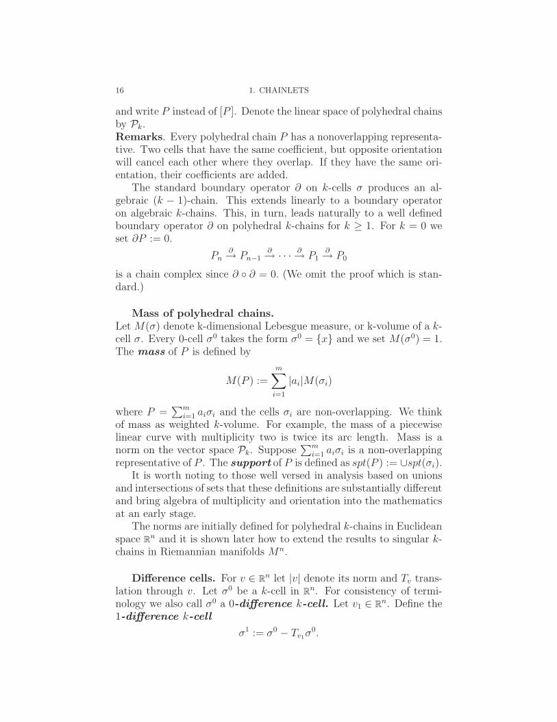
and write P instead of [P ]. Denote the linear space of polyhedral chainsby Pk.Remarks. Every polyhedral chain P has a nonoverlapping representa-tive. Two cells that have the same coefficient, but opposite orientationwill cancel each other where they overlap. If they have the same ori-entation, their coefficients are added.

The standard boundary operator ∂ on k-cells σ produces an al-gebraic (k − 1)-chain. This extends linearly to a boundary operatoron algebraic k-chains. This, in turn, leads naturally to a well definedboundary operator ∂ on polyhedral k-chains for k ≥ 1. For k = 0 weset ∂P := 0.

Pn∂→ Pn−1

∂→ · · · ∂→ P1∂→ P0

is a chain complex since ∂ ∂ = 0. (We omit the proof which is stan-dard.)

Mass of polyhedral chains.

Let M(σ) denote k-dimensional Lebesgue measure, or k-volume of a k-cell σ. Every 0-cell σ0 takes the form σ0 = x and we set M(σ0) = 1.The mass of P is defined by

M(P ) :=

m∑

i=1

|ai|M(σi)

where P =∑m

i=1 aiσi and the cells σi are non-overlapping. We thinkof mass as weighted k-volume. For example, the mass of a piecewiselinear curve with multiplicity two is twice its arc length. Mass is anorm on the vector space Pk. Suppose

∑mi=1 aiσi is a non-overlapping

representative of P . The support of P is defined as spt(P ) := ∪spt(σi).It is worth noting to those well versed in analysis based on unions

and intersections of sets that these definitions are substantially differentand bring algebra of multiplicity and orientation into the mathematicsat an early stage.

The norms are initially defined for polyhedral k-chains in Euclideanspace R

n and it is shown later how to extend the results to singular k-chains in Riemannian manifolds Mn.

Difference cells. For v ∈ Rn let |v| denote its norm and Tv trans-

lation through v. Let σ0 be a k-cell in Rn. For consistency of termi-

nology we also call σ0 a 0-difference k-cell. Let v1 ∈ Rn. Define the

1-difference k-cell

σ1 := σ0 − Tv1σ0.

POLYHEDRAL CHAINS 17

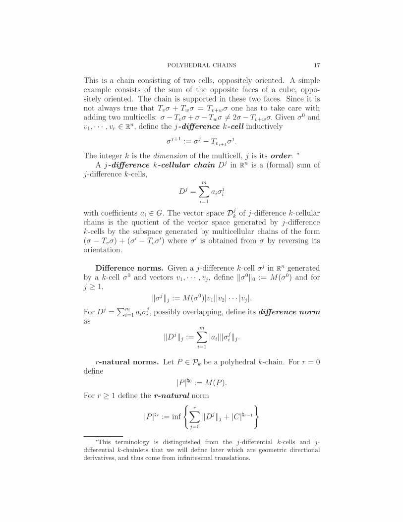
This is a chain consisting of two cells, oppositely oriented. A simpleexample consists of the sum of the opposite faces of a cube, oppo-sitely oriented. The chain is supported in these two faces. Since it isnot always true that Tvσ + Twσ = Tv+wσ one has to take care withadding two multicells: σ − Tvσ + σ −Twσ 6= 2σ− Tv+wσ. Given σ0 andv1, · · · , vr ∈ R

n, define the j-difference k-cell inductively

σj+1 := σj − Tvj+1σj .

The integer k is the dimension of the multicell, j is its order. ∗

A j-difference k-cellular chain Dj in Rn is a (formal) sum of

j-difference k-cells,

Dj =

m∑

i=1

aiσji

with coefficients ai ∈ G. The vector space Djk of j-difference k-cellular

chains is the quotient of the vector space generated by j-differencek-cells by the subspace generated by multicellular chains of the form(σ − Tvσ) + (σ′ − Tvσ

′) where σ′ is obtained from σ by reversing itsorientation.

Difference norms. Given a j-difference k-cell σj in Rn generated

by a k-cell σ0 and vectors v1, · · · , vj, define ‖σ0‖0 := M(σ0) and forj ≥ 1,

‖σj‖j := M(σ0)|v1||v2| · · · |vj |.For Dj =

∑mi=1 aiσ

ji , possibly overlapping, define its difference norm

as

‖Dj‖j :=

m∑

i=1

|ai|‖σji ‖j.

r-natural norms. Let P ∈ Pk be a polyhedral k-chain. For r = 0define

|P |0 := M(P ).

For r ≥ 1 define the r-natural norm

|P |r := inf

r∑

j=0

‖Dj‖j + |C|r−1

∗This terminology is distinguished from the j-differential k-cells and j-differential k-chainlets that we will define later which are geometric directionalderivatives, and thus come from infinitesimal translations.

18 1. CHAINLETS

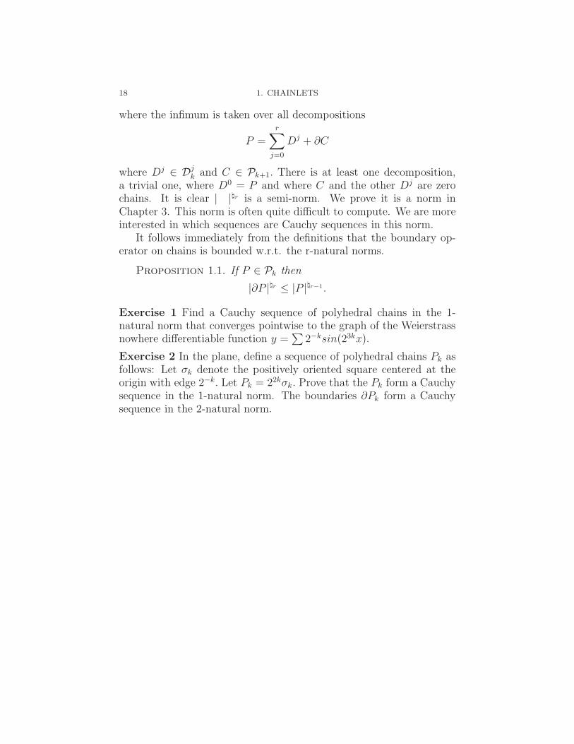
where the infimum is taken over all decompositions

P =

r∑

j=0

Dj + ∂C

where Dj ∈ Djk and C ∈ Pk+1. There is at least one decomposition,

a trivial one, where D0 = P and where C and the other Dj are zerochains. It is clear | |r is a semi-norm. We prove it is a norm inChapter 3. This norm is often quite difficult to compute. We are moreinterested in which sequences are Cauchy sequences in this norm.

It follows immediately from the definitions that the boundary op-erator on chains is bounded w.r.t. the r-natural norms.

Proposition 1.1. If P ∈ Pk then

|∂P |r ≤ |P |r−1.

Exercise 1 Find a Cauchy sequence of polyhedral chains in the 1-natural norm that converges pointwise to the graph of the Weierstrassnowhere differentiable function y =

∑2−ksin(23kx).

Exercise 2 In the plane, define a sequence of polyhedral chains Pk asfollows: Let σk denote the positively oriented square centered at theorigin with edge 2−k. Let Pk = 22kσk. Prove that the Pk form a Cauchysequence in the 1-natural norm. The boundaries ∂Pk form a Cauchysequence in the 2-natural norm.

CHAPTER 2

Exterior algebra

k-vectors

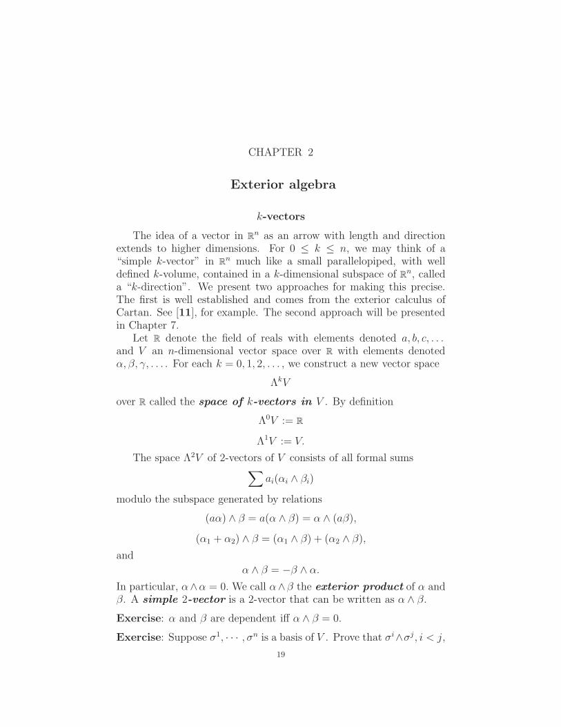
The idea of a vector in Rn as an arrow with length and direction

extends to higher dimensions. For 0 ≤ k ≤ n, we may think of a“simple k-vector” in R

n much like a small parallelopiped, with welldefined k-volume, contained in a k-dimensional subspace of R

n, calleda “k-direction”. We present two approaches for making this precise.The first is well established and comes from the exterior calculus ofCartan. See [11], for example. The second approach will be presentedin Chapter 7.

Let R denote the field of reals with elements denoted a, b, c, . . .and V an n-dimensional vector space over R with elements denotedα, β, γ, . . . . For each k = 0, 1, 2, . . . , we construct a new vector space

ΛkV

over R called the space of k-vectors in V . By definition

Λ0V := R

Λ1V := V.

The space Λ2V of 2-vectors of V consists of all formal sums∑

ai(αi ∧ βi)

modulo the subspace generated by relations

(aα) ∧ β = a(α ∧ β) = α ∧ (aβ),

(α1 + α2) ∧ β = (α1 ∧ β) + (α2 ∧ β),

and

α ∧ β = −β ∧ α.

In particular, α∧α = 0. We call α∧β the exterior product of α andβ. A simple 2-vector is a 2-vector that can be written as α ∧ β.

Exercise: α and β are dependent iff α ∧ β = 0.

Exercise: Suppose σ1, · · · , σn is a basis of V . Prove that σi∧σj , i < j,

19

20 2. EXTERIOR ALGEBRA

forms a basis of Λ2V. Hence dimΛ2V =

(n2

)

(See [11], for example, for details) The space Λk(V ) of k-vectors ofV , 2 < k ≤ n, is defined recursively. A k-vector is a formal sum

∑aiαi ∧ βi

where αi ∈ Λk−1(V ) is a simple (k − 1)-vector and βi ∈ V , subject tothe constraints

(aα) ∧ β = a(α ∧ β) = α ∧ (aβ),

(α1 + α2) ∧ β = (α1 ∧ β) + (α2 ∧ β),

andα ∧ β = (−1)k−1β ∧ α.

We set ΛkV = 0 for all k > n.If k ≤ n a basis for ΛkV consists of k-vectors of the form

σ11 ∧ σi2 ∧ · · · ∧ σik

where i1 < i2 < · · · ik. Then dimΛkV =

(nk

)

The k-vector of a polyhedral chain. ([2], III) A k-cell σ de-termines a unique k-direction. This, together with its k-volume M(σ)determine a unique simple k-vector denoted V ec(σ) with the same massand direction. Define the k-vector of an algebraic k-chain A =

∑aiσi

by V ec(A) :=∑

aiV ec(σi). For k = 0 define V ec(∑

aipi) :=∑

ai.This definition extends to a polyhedral k-chain P since the k-vector ofany chain equivalent to a k-cell is the same as the k-vector of the k-cell.The main purpose of introducing V ec(A) in this paper is to show thatthe important k-elements defined below in Chapter 7 are, in fact, welldefined.

Proposition 2.1. If P is a polyhedral k-chain then V ec(∂P ) = 0.

Proof. This follows since V ec(∂σ) = 0 for every k-cell σ.

Theorem 2.2. V ec is a linear operator

V ec : Pk → Λk(Rn)

withM(V ec(P )) ≤ M(P )

for all P ∈ Pk.

Proof. This follows since M(V ec(σ)) = M(σ) for every k-cell σ.

INNER PRODUCT SPACES 21

Exterior product of j- and k-vectors. Define

∧ : (ΛjV ) × (ΛkV ) → Λj+kV

by

∧(α1 ∧ · · · ∧ αj , β1 ∧ · · · ∧ βk) = α1 ∧ · · · ∧ αj ∧ β1 ∧ · · · ∧ βk.

This product is distributive, associative and anticommutative:

µ ∧ λ = (−1)jkλ ∧ µ.

Exercise: Prove that all k-vectors in Λk(Rn) are simple k-vectors forn ≤ 3. Show this fails for n = 4 by showing that (e1 ∧ e2) + (e3 ∧ e4) isnot simple.

Oriented k-direction of a simple k-vector. Define thek-direction of a simple k-vector α to be the k-dimensional subspaceof the vectors α1, · · · , αk that determine α = α1 ∧ α2 ∧ · · · ∧ αk. Thissubspace inherits an orientation from α as follows: Two bases of avector space V are equivalent if and only if the matrix relating themhas positive determinant. An equivalence class of bases is called anorientation. There are only two orientations of V and we chooseone of them and fix it, once and for all. We say a basis is positively

or negatively oriented, according as to whether it has the chosenorientation. A subspace of V has no preferred orientation but it makessense to give the k-direction of a simple k-vector the same or oppositeorientation as α. If we give it the same orientation as α, we obtain theoriented k-direction of α.

Standard operators on V such as linear transformations, inner prod-ucts and determinants naturally extend to corresponding structuresand operators on ΛkV. For example, if T : V → W is linear then thetransformation Λk(T ) : Λk(V ) → Λk(W ) defined on simple k-vectorsα = α1 ∧ α2 ∧ · · · ∧ αk by

ΛkT (α) = T (α1) ∧ T (α2) ∧ · · · ∧ T (αk)

is linear. Extend ΛkT to k-vectors by linearity.

Inner product spaces

An inner product on a vector space V is a real-valued function onV × V which is symmetric positive definite bilinear form. An exampleis the Euclidean inner product on R

n given by < α, β >=∑

aibi

where α = (a1, · · ·an) and β = (b1, · · · bn). An orthonormal basis ofV consists of a basis σ1, · · · , σn such that

< σi, σj >= δij .


Suppose V is an inner product space. We define an inner product forsimple vectors α, β ∈ ΛkV as follows:

< α, β >:= det(< αi, βj >)

where α = α1 ∧α2 ∧ · · ·αk and β = β1 ∧ β2 ∧ · · ·βk. Since determinantis an alternating, k-multilinear function of the α′s and β ′s we obtain ascalar valued function, linear in each variable

< , >: ΛkV × ΛkV → R.

Note that < α, β >=< β, α > since the determinant of the transposeof a matrix is the same as the determinant of the matrix.

It is left to show that the inner product is well defined.

Orthonormal basis of ΛkV . Choose an orthonormal basis e1, · · · enof V . For H = h1, h2, · · · , hk, let

eH := eh1 ∧ eh2 ∧ · · · ∧ ehk .

Then the collection of simple k-vectors

eH : H = h1 < h2 < · · · < hk

forms a basis of ΛkV.

Mass of α. For a simple k-vector α, define M(α) =√

< α, α >.

Volume elements. If V is an inner product space, the volumeelement vol is well defined (with respect to the chosen orientation). Itis the unique n-vector in ΛnV with

vol = e1 ∧ e2 ∧ · · · ∧ en

where (ei) is a positively oriented orthonormal basis. Observe thatM(vol) = 1.

Exercise eH is an orthonormal basis of ΛkV. (Hint: H 6= L =⇒ thematrix has a row of zeroes. H = L =⇒ all but the diagonal elementsvanish. Thus < eH , eJ >= ±1 if H and J contain the same indices withno repeats, and is zero, otherwise. In particular, vol = e1 ∧ · · · ∧ en isan orthonormal basis of ΛnV and < vol, vol >= 1.

The k-vector Pk of each Pk in exercise of Chapter 1 is the volumeelement in R

2.

TWO BASIC EXAMPLES 23

Two basic examples

Example 1. The oriented k-direction of an oriented k-dimensional par-ellelopiped P is the oriented k-subspace generated by the vectors thatdetermine P . We create equivalence classes of oriented k-parallelopipedsP in R

n. We say that P ∼ Q if P and Q have the same k-volume andoriented k-direction. We take formal sums of these classes to form avector space Pk. Clearly, there is a 1-1 correspondence between simplek-vectors and equivalence classes of parallelopipeds with a given ori-ented k-direction and k-volume, or mass. The notion of taking productsof k-vectors and making k-parallelograms justifies the use of the termbfserires itshape exterior product since the k-parallelogram takes upspace exterior to its defining vectors. Later, we will see an interiorproduct where the parallelogram created is interior to its defining vec-tors. The term exterior, associated to the first definition given in thesenotes, the exterior product, is used throughout the subject. We willsee exterior derivatives, exterior algebra, exterior chainlets. Each timeyou see the term you should expect to see the exterior product playinga major role. For example the exterior algebra is called an algebrabecause it comes with a product, namely the exterior product.

Theorem 2.3. There is a canonical isomorphism

Θ : Λk(Rn) → Pk

such that the k-dimensional volumes and oriented k-directions of P andΘ(P ) are the same.

We assume all k-vectors and k-directions are oriented and usuallyomit the term “oriented”.

This result gives us a simple geometric way to view Λk(Rn) andwill help us visualize operators and products as we go along. However,an important feature missing from this representation is that there isno canonical representative of a k-vector within a class of parallelop-ipeds. In particular, one cannot define the boundary of a k-vector. Animportant goal of these notes is to resolve this problem.

Example 2. The differential dxi of Rn is defined to be the linear

functional on Rn given by dxi(x1e1 + · · · + xnen) := xi. Let Dn denote

the linear space generated by differentials dx1, dx2, · · · , dxn of Rn.

The space Λk(Dn) is of special interest. We follow the common practiceof omitting the wedge sign for k-vectors e.g., dxi∧dxj = dxidxj. Thesek-vectors of differentials exist since they do so for any vector space.The theorem tells us what they are – linear functionals of k-vectors ofR

n.


Theorem 2.4. The mapping aHdxH 7→ aHeH induces an isomor-phism

Λk(Dn) ∼= (ΛkR

n)′.

Differential forms

A differential k-form ω on U ⊂ Rn is an element of the dual

space of Λk(Rn) for each p ∈ U,

ω : U × Λk(Rn) → R.

∗ In these notes, we define three basic operators on forms as dual tocorresponding operators on k-vectors: Hodge star ∗ω, pullback f ∗ωand exterior derivative dω :

• ⋆ω(p, α) := ω(p, ⋆α)• f ∗ω(p, α) := ω(p, f∗α)• dω(p, α) := ω(p, ∂α)

We are reduced to defining three geometric operators on simple k-vectors α ∈ Λk(Rn) – the star operator ⋆α, pushforward f∗α and bound-ary ∂α. Star of a simple k-vector will be presented in this section. Wepostpone defining the boundary ∂α of a simple k-vector α until thelecture on discrete calculus. The idea of the boundary of a k-vector isa new and important concept introduced in these notes.

Theorem 2.5. If T : Rn → R

n is a linear transformation andα ∈ Λk(Rn) then

Λk−1T (∂α) = ∂(ΛkT (α)).

The definitions and proof will be postponed until Lecture III as thenatural norm is needed to define the boundary of a k-vector in Lk(Rn).

Pullback of a differential form. Suppose f : U ⊂ Rn → V ⊂ R

m

is smooth. Denote the Jacobian matrix of partial derivatives evaluatedat p ∈ U by Dfp. This, of course is a linear transformation Dfp : R

n →R

m. We will denote

Dkfp := Λk(Dfp) : Λk(Rn) → Λk(Rn).

∗In GC we define operators on differential forms as dual to geometric operatorson k-vectors α defined at each point, without integrating, whereas GMT definesoperators on domains (currents) as dual to operators defined analytically on differ-ential forms.

DIFFERENTIAL FORMS 25

Observe that if α is a k-vector then Dkfp(α) is a well defined k-vectorcalled the pushforward of α under f . The pullback of a k-form ω inV is a k-form f ∗ω in U defined by

f ∗ω(p, α) := ω(f(p), Dkfp(α)).

Lemma 2.6. If f : U ⊂ Rn → V ⊂ R

m is smooth and ω is adifferential k-form then

(1) f ∗(ω + η) = f ∗ω + f ∗η;(2) f ∗(α ∧ β) = f ∗α ∧ f ∗β;(3) df ∗ = f ∗d(4) (g f)∗ = f ∗ g∗

Proof.

(1) follows since Dkfp is linear.(2) follows since Dkfp acts on a k-vector α = α1 ∧ · · · ∧αk by way

of the linear transformation Dfp applied to each αi.(3)

df ∗ω(p, α) = f ∗ω(p, ∂(α)) = ω(f(p), Dk−1fp(∂α)).

On the other hand, by Theorem 2.5

f ∗dω(p, α) = dω(f(p), Dkfp(α)) = ω(f(p), ∂Dkfp(α))

= ω(f(p), Dkfp(∂α)).

(4)

(g f)∗ω(p, α) = ω(g f(p), Dk(g f)p(α))

= ω(g f(p), Dkgf(p)Dkfp(α))

= f ∗ g∗ω(p, α).

Examples. 1. Let f : R2 → R be defined by f(x, y) = x − y and

ω = dt a 1-form on R. Then

f ∗ω((x, y), (a1, a2)) = ω(f(x, y), Dfx,y(a1, a2))

= dt(x − y, a1 − a2)

= a1 − a2 = (dx − dy)(a1, a2).

Therefore f ∗dt = dx − dy.Remark. The standard approach (commonly unjustified) is

t = x − y =⇒ dt = dx − dy.


2. Let f(t) : R1 → R

2 be defined by f(t) = (t2, t3). Let ω be the1-form in R

2 given by ω = xdy. Then

f ∗ω(t, 1) = ω(f(t), Dft(1))

= ω((t2, t3), (2t, 3t2))

= xdy((t2, t3), (2t, 3t2))

= t23t2

= 3t4dt(t, 1).

Therefore f ∗(xdy) = 3t4dt.

Hodge star dual. Given a simple k-vector α, we wish to find acanonical simple (n − k)-vector ⋆α such that α ∧ ⋆α = M(α)2vol.

We further require that the (n−k)-direction of ⋆α be perpendicularto the k-direction of α. We are reduced to showing existence anduniqueness.

For this, we recall the Riesz representation theorem:

Theorem 2.7. Suppose V is an inner product space and f ∈ V ∗ isa linear functional. There exists a unique w ∈ V such that

f(v) =< v, w > .

Proof. Let e1, · · · , en be orthonormal. Set bi := f(ei). Set w =∑bje

j . Then < ei, w >= bi = f(ei).

Now fix α ∈ ΛkV . For β ∈ Λn−k the mapping β 7→ α∧ β is a lineartransformation

Λn−k → Λn.

The latter space has dimension one. Therefore one may define fα(β)by

α ∧ β = fα(β)vol

where fα is a linear functional on Λn−kV. According to Theorem 2.7there exists a unique (n − k)-vector ⋆α such that

α ∧ µ =< ⋆α, µ > vol

for all µ ∈ Λn−k.

Lemma 2.8. For simple α the (n − k)-direction of ⋆α is the or-thogonal complement of the k-direction of α, oriented so that α∧ ⋆α ispositively oriented.

DIFFERENTIAL FORMS 27

In particular

α ∧ ⋆α = (−1)k(n−k) ⋆ α ∧ α = (−1)k(n−k) < ⋆ ⋆ α, α > vol

= (−1)k(n−k)(−1)k(n−k) < α, α > vol = M(α)2vol.

Lemma 2.9. If α, β are k-vectors then

(1) ⋆ ⋆ α = (−1)k(n−k)α.(2) α ∧ ⋆β = β ∧ ⋆α =< α, β > vol

If ω is a differential k-form, define the Hodge star dual ⋆ω as

⋆ω(p, α) := ω(p, ⋆α)

for all (n−k)-vectors α. If ω is a k-form we know that ω = ω1∧· · ·∧ωk

where the ωi are 1-forms. Each ωi corresponds to a vector wi from theabove exercise.

Proposition 2.10. Assume ω = ω1 ∧ · · · ∧ ωk is a simple k-form.Then (⋆ω)(v1∧· · ·∧vn−k) is the volume of the n-parallelogram spannedby v1, · · · , vn−k, w1, · · ·wk.

CHAPTER 3

Differential forms and chainlets

Isomorphisms of differential forms and cochains

We recall two classical results from integral calculus:

Theorem 3.1 (Classical Stokes’ theorem). If P is a polyhedral k-chain and ω is a smooth k-form defined in a neighborhood of P then

∫

∂P

ω =

∫

P

dω.

Theorem 3.2 (Classical change of variables). If P is a polyhedralk-chain, ω is a smooth k-form and f is an orientation preserving dif-feomorphism defined in a neighborhood of P then

∫

fP

ω =

∫

P

f ∗ω.

The flat norm. Whitney’s flat norm [2] on polyhedral chains A ∈Pk is defined as follows:

|A| = infM(B) + M(C) : A = B + ∂C, B ∈ Pk, C ∈ Pk+1.Flat k-forms ([2], 12.4) are characterized as all bounded mea-

surable k-forms ω such that there exists a constant C > 0 such thatsup |

∫σω| < CM(σ) for all k-cells σ and sup |

∫∂τ

ω| < CM(τ) for all(k + 1)-cells τ . The exterior derivative dω of a flat form ω is defineda.e. and satisfies ∫

∂τ

ω =

∫

τ

dω.

Exercises

1. Prove that the form

ω =

dx − dy, x > y

0, x ≤ y

is flat but the form

η =

dx + dy, x > y

0 x ≤ y

29

30 3. DIFFERENTIAL FORMS AND CHAINLETS

is not flat. (Hint. Consider small squares with centers on the diagonal.)Thus ω is smoothly homotopic to a form that is not flat. Show thatthere are forms arbtirarily close to ω that are not flat. Show that thecomponents of ω are not flat.

We conclude that the flat topology is limited at the level of chainsand cochains. (Comment for experts: Some problems disappear at thelevel of homology and cohomology.)

2. Let P be the boundary of a rectangle with bottom edge length10 and side length 0.1. Let Q be the same curve without one of theshort edges. Show that |P | < |Q|.

The support of a differential form is the closure of the set of allpoints p ∈ R

n such that ω(p) is nonzero. Let U be an open subset ofR

n and ω be a bounded measurable k-form whose support is containedin U . In what follows, let σ denote a k-cell and τ a (k + 1)-cell.

Define

‖ω‖0 := sup

∫σω

M(σ): σ ⊂ sptω

.

Inductively define

‖ω‖r := sup

‖ω − Tvω‖r−1

|v| : spt(ω − Tvω) ⊂ U

.

Define

‖ω‖′0 := sup

∫∂τ

ω

M(τ): τ ⊂ sptω

and

‖ω‖′r := sup

‖ω − Tvω‖′r−1

|v| : spt(ω − Tvω) ⊂ U

.

Define

|ω|0 := ‖ω‖0

and for r ≥ 1,

|ω|r := max‖ω‖o, · · · , ‖ω‖r, ‖ω‖′0, · · · , ‖ω‖′r−1.We say that ω is of class Br if |ω|r < ∞. Let Br

k denote the space ofdifferential k-forms of class Br.

Lemma 3.3. If |ω|1 < ∞ then dω is defined a.e. Furthermore,∫

∂σ

ω =

∫

σ

dω

Proof. If |ω|1 < ∞ then ω is a flat form. It follows from ([2],12.4) that dω is defined a.e. and satisfies Stokes’ theorem on cells.

ISOMORPHISMS OF DIFFERENTIAL FORMS AND COCHAINS 31

Lemma 3.4. If ω ∈ Brk, r ≥ 1, then

|ω|r = max‖ω‖o, · · · , ‖ω‖r, ‖dω‖0, · · · , ‖dω‖r−1.Therefore

(1) |dω|r−1 ≤ |ω|r.Remark. On a smooth manifold these norms are equivalent to the

Cr−1+Lip norms of analysis. That is, the (r − 1)-derivatives exist andsatisfy Lipschitz conditions. However, the norms can also be definedon Lipschitz manifolds where one cannot speak of higher derivatives.We only know that derivatives of Lipschitz functions exist almost ev-erywhere. However, a constant function is of class Br for all r, even ona Lipschitz manifold. This opens the possibility of extending chainletgeometry to Lipschitz Riemannian manifolds which we will develop in alater chapter. (We must be able to define divergence free vector fields,exterior derivative and star operator a.e.)

The next result generalizes the standard integral inequality of cal-culus: ∣∣∣∣

∫

P

ω

∣∣∣∣ ≤ M(P )|ω|owhere P is polyhedral and ω is a bounded, measurable form.

Theorem 3.5 (Fundamental integral inequality of chainlet geome-try). Let P ∈ Pk, r ∈ Z

+, and ω ∈ Brk be defined in a neighborhood of

spt(P ). Then ∣∣∣∣∫

P

ω

∣∣∣∣ ≤ |P |r |ω|r.

Proof. We first prove∣∣∫

σj ω∣∣ ≤ ‖σj‖j‖ω‖j. Since ‖ω‖0 = |ω|0 we

know ∣∣∣∣∫

σ0

ω

∣∣∣∣ ≤ M(σ0)|ω|0 = ‖σ0‖0‖ω‖0.

Use the change of variables formula 3.2 for the translation Tvjand

induction to deduce∣∣∫

σj ω∣∣ =

∣∣∣∫

σj−1−Tvjσj−1 ω

∣∣∣ =∣∣∣∫

σj−1 ω − T ∗vj

ω∣∣∣

≤ ‖σj−1‖j−1‖ω − T ∗vj

ω‖j−1

≤ ‖σj−1‖j−1‖ω‖j|vj |= ‖σj‖j‖ω‖j

By linearity ∣∣∣∣∫

Dj

ω

∣∣∣∣ ≤ ‖Dj‖j‖ω‖j


for all Dj ∈ Djk.

We again use induction to prove∣∣∫

Pω∣∣ ≤ |P |r |ω|r. We know

∣∣∫P

ω∣∣ ≤

|P |0|ω|0. Assume the estimate holds for r − 1.Let ε > 0. There exists P =

∑rj=0 Dj + ∂C such that |P |r >∑r

j=0 ‖Dj‖j + |C|r−1 − ε. By Stokes’ theorem for polyhedral chains,

inequality (1) and induction∣∣∫

Pω∣∣ ≤ ∑r

j=0

∣∣∫Dj ω

∣∣ + |∫

Cdω|

≤ ∑rj=0 ‖Dj‖j‖ω‖j + |C|r−1|dω|r−1

≤ (∑r

j=0 ‖Dj‖j + |C|r−1)|ω|r≤ (|P |r + ε)|ω|r.

Since the inequality holds for all ε > 0 the result follows.

Corollary 3.6. |P |r is a norm on the space of polyhedral chainsPk.

Proof. Suppose P 6= 0 is a polyhedral chain. There exists asmooth differential form ω such that

∫P

ω 6= 0. Then 0 <∣∣∫

Pω∣∣ ≤

|P |r |ω|r implies |P |r > 0.

The Banach space of polyhedral k-chains Pk completed with thenorm | |r is denoted N r

k . The elements of N rk are called k-chainlets

of class N r.It follows from Proposition 1.1 that the boundary ∂A of a k-chainlet

A of class N r is well defined as a (k − 1)-chainlet of class N r+1. IfPi → A in the r-natural norm define

∂A := limi→∞

∂Pi.

By Theorem 3.5 the integral∫

Aω is well defined for k-chainlets A of

class N r and differential k-forms of class Br. If Pi → A in the r-naturalnorm define ∫

A

ω := limi→∞

∫

Pi

ω.

Theorem 3.7. [Generalized Stokes’ theorem] If A is a k-chainlet ofclass N r and ω is a (k−1)-form of class Br+1 defined in a neighborhoodof sptA then ∫

∂A

ω =

∫

A

dω.

Proof. Choose polyhedral Pi → A in the r-natural norm. ByStokes’ theorem for polyhedral chains∫

A

dω = lim

∫

Pi

dω = lim

∫

∂Pi

ω = lim

∫

∂A

ω.

THE BANACH SPACE N Ik OF CHAINLETS 33

Later, in the discrete chapter, we give a proof without relying onthe classical Stokes’ theorem for polyhedral chains.

Examples of chainlets

(1) The boundary of any bounded, open subset U of Rn.

One may easily verify that the boundary of any bounded, openset U ⊂ R

n, such as the Van Koch snowflake, supports a welldefined chainlet B = ∂U of class N1. Suppose the frontier of Uhas positive Lebesgue area. Then the chainlet B′ = ∂(Rn −U)has the same support as B, namely the frontier of U , but sinceB + B′ bounds a chainlet with positive mass it follows that Band −B′ are distinct.

(2) Graphs of functions The graph of a nonnegative L1 func-tion f : K ⊂ R

n → R supports a chainlet Γf if K is compact.This can be seen by approximating Γf by the polyhedral chainsPk determined by a sequence of step functions gk approximat-ing f . The difference Pk − Pk+j is a 1-difference k-cellularchain. The subgraph of a nonnegative function f is the areabetween the graph of f and its domain. Since the subgraph off has finite area, it follows that ‖Pk−Pk+j‖1 → 0 as j, k → ∞.Hence, the sequence Pk is Cauchy in the 1-natural norm. Theboundary ∂Γf is a chainlet that identifies the discontinuitypoints of f .

Later, we will define the natural norms and develop a full theoryof integration from first principles, without reference to the classicalStokes’ theorem or even the Riemann integral.

The Banach space N∞k of chainlets

It can be easily shown that the r-natural norms satisfy the inequal-ities

|P |0 ≥ |P |1 ≥ |P |2 ≥ · · ·for any polyhedron P . It follows that there are natural inclusion map-pings ηr : N r

k → N r+1k defined as follows: If A ∈ N r

k then A = lim Pj

in the r-natural norm. Define ηr(A) := lim Pj in the (r + 1)-naturalnorm.

For P a polyhedral chain define

|P | := limr→∞

|P |r .

This limit exists since the r-natural norms are decreasing.

Theorem 3.8. | | is a norm on polyhedral chains.


Proof. If P, Q ∈ N∞k then

|P + Q| = limr→∞ |P + Q|r

≤ lim supr→∞(|P |r + |Q|r)= limr→∞ |P |r + limr→∞ |Q|r

= |P | + |Q|

and

|λP | = limr→∞

|λP |r = |λ| limr→∞

|P |r = |λ||P |.

Clearly, P = 0 =⇒ |P | = 0. It remains to show |P | 6= 0 =⇒ P 6= 0for a polyhedron P . But if P is a nonzero polyhedral chain, thereexists a smooth form ω and a constant C > 0 such that

∫P

ω 6= 0 and

|ω|r < C for all r. Then 0 <∣∣∫

Pω∣∣ ≤ |P |r |ω|r < C|P |r for each r. It

follows that |P | ≥∣∣∫

Pω∣∣ /C > 0.

We call elements of the Banach space N∞k obtained upon comple-

tion k-chainlets of class N∞ or, more simply, k-chainlets.

Theorem 3.9. If A is a chainlet in Rn and v ∈ R

n then

|A − TvA| ≤ |v||A|.Hence translation of a chainlet converges uniformly to 0 as a func-

tion of A and v.

Proof. Let Pi → A. Then Pi − TvPi → A − TvA. It follows that

|A − TvA| = lim |Pi − TvPi| ≤ |v||Pi| → |v||A|.

Theorem 3.10.

|∂A| ≤ |A| .Proof.

|∂A| = limr→∞

|∂A|r ≤ limr→∞

|A|r−1 = |A| .

In these lectures we introduce a number of operators on chainletsall of which are bounded in the chainlet spaces. The Banach spacesof chainlets are not reflexive since they are separable and differentialforms are not separable [7]. Thus N is strictly contained in (N )∗∗.Now operators dual to operators on differential forms automaticallysend chainlets into the double dual space. It is surprising that theoperators map N into itself.


Characterization of the Banach space of chainlets.

Theorem 3.11. Suppose | |′ is a seminorm of polyhedral chainssatisfying

(1) |∂D0|′ ≤ |D0|r−1 and(2) |Di|′ ≤ ‖Di‖i for all multicellular chains Di and 0 ≤ i ≤ r.

Then |P |′ ≤ |P |r for all polyhedral chains P .

Proof. For r ≥ 1, if ε > 0 there exists a decomposition P =∑ri=0 Di + ∂C such that

|P |r >r∑

i=0

‖Di‖i + |C|r−1 − ε.

By assumption

|P |′ ≤r∑

i=0

|Di|′ + |∂C|′ ≤r∑

i=0

‖Di‖i + |C|r−1 < |P |r + ε.

The result follows

Corollary 3.12.

|A|r = inf

r∑

i=0

‖Di‖i + |C|r−1 : A =r∑

i=0

Di + ∂C, Di ∈ N r , C ∈ N r−1

.

Proof. Denote the rhs by |A|<r>. This is clearly a seminorm. Bythe characterization of the r-natural norm, we know that |A|<r> ≤|A|r .

Let ε > 0. There exists A =∑

Di + ∂C, Di ∈ N r , C ∈ N r−1 suchthat

|A|<r> >r∑

i=0

‖Di‖i + |C|r−1 − ε.

Then|A|r ≤

∑|Di|r + |C|r−1

=∑

|Di|r + |C|r−1

≤∑

|Di|i + |C|r−1

≤∑

‖Di‖i + |C|r−1

< |A|<r> + ε.

Corollary 3.13. The natural norm is the largest seminorm in theclass of seminorms satisfying


(1) |A|′ ≤ M(A),(2) |∂A|′ ≤ |A|′ and(3) |A − TvA|′ ≤ |v||A|′.

Proof. First observe that conditions (1) and (3) imply |Di|′ ≤‖Di‖i for all multicellular chains Di and 0 ≤ i ≤ r. We know |D0|′ ≤‖D0‖0 by (1). Assume the claim holds for i−1. By (3) and the inductionhypothesis

|σi|′ = |σi−1 − Tvσi−1|′ ≤ |v||σi−1|′ ≤ |v|‖σi−1‖i−1 = ‖σi‖i.

The claim is established by taking linear combinations.Let P be a polyhedral chain. Given ε > 0 there exists r such that

|P | > |P |r − ε/2

and a decomposition P =∑

Di + ∂C such that

|P |r >∑

‖Di‖i + |C|r−1 − ε/2.

Hence|P | >

∑‖Di‖i + |C|r−1 − ε.

If k = n then the same inequality holds, except we set C = 0 since Chas dimension n + 1. In this case we have

|P |′ ≤∑

|Di|′ ≤∑

‖Di‖i < |P | + ε.

Since the result holds for all ε > 0 we conclude |P |′ ≤ |P |. Nowassume the result holds for polyhedral k-chains C, we prove it holdsfor polyhedral (k − 1)-chains P .

Thus by induction

|P |′ ≤∑

|Di|′ + |∂C|′

≤∑

‖Di‖i + |C|′

≤∑

‖Di‖i + |C|

≤∑

‖Di‖i + |C|r−1

< |P | + ε.

Let X be a Banach space with norm | |′. We say an operatorS : X → X is is Lipschitz bounded if there exists K > 0 suchthat |S(A)|′ ≤ K|A|′ for all A ∈ X. An operator S : X × R

n → Xis Lipschitz bounded if there exists K > 0 such that |S(A, v)|′ ≤K|v||A|′ for all A ∈ X and v ∈ Rn. Two examples that interest us are


the translation operator S(A, v) = A−TvA and the boundary operatorS(A) = ∂A. We assume K = 1 in what follows as different constantslead to the same Banach space.

Let X0 be the completion of the space of polyhedral chains withthe mass norm.

Corollary 3.14. The Banach space of chainlets is the smallestBanach space containing X0 and which has Lipschitz bounded boundaryand translation operators.

Characterization of cochains as differential forms. The r-natural norm of a cochain X ∈ (N r)′ is defined by

|X|r := supP∈P

|X · P ||P |r

.

The differential operator d on cochains is defined as the dual to theboundary operator dX ·A := X · ∂A. It remains to show how cochainsrelate to integration of differential forms and how the operator d givenabove relates to the standard exterior derivative of differential forms.If X ∈ (N r

k )′ then dX ∈ (N r−1k+1 )′ by Lemma 1.1.

Cochains and differential forms. In this section we show theoperator Ψ mapping differential forms of class Br into the dual spaceof chainlets of class N r via integration

Ψ(ω) · A :=

∫

A

ω

is a norm preserving isomorphism of graded algebras.It follows from Theorem 3.5 thatΨ(ω) ∈ (N r

k )′ with

|Ψ(ω)|r ≤ |ω|r.Theorem 3.15 (Extension of the theorem of de Rham). Let r ≥ 0.

To each cochain X ∈ (N rk )′ there corresponds a unique differential

form φ(X) ∈ Brk such that

∫σφ(X) = X · σ for all cells σ. This

correspondence is an isomorphism with

|X|r = |φ(X)|r.If r ≥ 1 then

φ(dX) = dφ(X).

This is proved in [8].

Corollary 3.16. If A, B ∈ N rk satisfy

∫

A

ω =

∫

B

ω


for all ω ∈ Brk then A = B.

Proof. Let X ∈ (N rk )′. By Theorem 3.15 the form φ(X) is of class

Br. Hence

X · (A − B) =

∫

A−B

φ(X) = 0.

It follows that A = B.

Corollary 3.17. If A ∈ N rk then

|A|r = sup

∫

A

ω : ω ∈ Brk, |ω|r ≤ 1

.

Proof. By Theorem 3.15

|A|r = sup

|X·A||X|r

: X ∈ (N rk )′

= sup

|∫

Aφ(X)|

|φ(X)|r: φ(X) ∈ Br

k

= sup

|∫

Aω|

|ω|r: ω ∈ Br

k

.

Cup product. Given a k-cochain X and a j-cochain Y , we definetheir cup product as the (j + k)-cochain

X ∪ Y := Ψ(φ(X) ∧ φ(Y )).

The next result follows directly from Theorem 3.15.

Lemma 3.18. Given X ∈ (N rk )′ and Y ∈ (N r

j )′ the cochain X∪Y ∈(N r

k+j(Rn))′ with

|X ∪ Y |r = |φ(X) ∧ φ(Y )|r.Furthermore

φ(X ∪ Y ) = φ(X) ∧ φ(Y ).

Theorem 3.19. If X ∈ (N rk )′, Y ∈ (N r

j )′, Z ∈ (N rℓ )′, and f ∈ Br+1

0

then

(i) |X ∪ Y |r ≤ |X|r |Y |r ;(ii) d(X ∪ Y ) = dX ∪ Y + (−1)j+kX ∪ dY ;(iii) (X ∪ Y ) + (Z ∪ Y ) = (X + Z) ∪ Y ; and(iv) a(X ∪ Y ) = (aX ∪ Y ) = (X ∪ aY ).

Proof. These follow by using the isomorphism of differential formsand cochains Theorem 3.15 and then applying corresponding results fordifferential forms and their wedge products.


Therefore the isomorphism Ψ of Theorem 3.15 is one on gradedalgebras.

Continuity of Vec(P).

Lemma 3.20. Suppose P is a polyhedral chain and ω is a bounded,measurable differential form. If ω(p) = ω0 for a fixed covector ω0 andfor all p, then ∫

P

ω = ω0 · V ec(P ).

Proof. This follows from the definition of the Riemann integral.

Theorem 3.21. If P is a polyhedral k-chain and r ≥ 1 then

M(V ec(P )) ≤ |P |r .

If spt(P ) ⊂ Bε(p) for some p ∈ Rn and ε > 0 then

|P |1 ≤ M(V ec(P )) + εM(P ).

Proof. Set α = V ec(P ) and let η0 be a covector such that |η0|0 =1, and η0 · α = M(α). Define the k-form η by η(p, β) := η0(β). Since ηis constant it follows that ‖η‖r = 0 for all r > 0 and ‖dη‖r = 0 for allr ≥ 0. Hence |η|r = |η|0 = |η0|0 = 1. By Lemma 3.20 and Theorem 3.5it follows that

M(V ec(P )) = η0 · V ec(P ) =

∫

P

η ≤ |η|r|P |r = |P |r .

For the second inequality we use Corollary 3.17. It suffices to show

that|∫

Pω|

|ω|1is less than or equal the right hand side for any 1-form ω of

class B1. Given such ω define the k-form ω0(q, β) := ω(p, β) for all q.By Lemma 3.20∣∣∣∣

∫

P

ω

∣∣∣∣ ≤∣∣∣∣∫

P

ω0

∣∣∣∣ +

∣∣∣∣∫

P

ω − ω0

∣∣∣∣≤ |ω(p) · V ec(P )| + sup

q∈sptP|ω(p) − ω(q)|M(P )

≤ ‖ω‖0M(V ec(P )) + ε‖ω‖1M(P )

≤ |ω|1(M(V ec(P )) + εM(P ))

If A = limi→∞ Pi in the r natural norm then Pi forms a Cauchysequence in the r-natural norm. By Theorem 3.21 V ec(Pi) forms aCauchy sequence in the mass norm on Λk(Rn). Define

V ec(A) := limV ec(Pi).


This is independent of the choice of approximating Pi, again by Theo-rem 3.21.

Corollary 3.22.

V ec : N rk → Λk(Rn)

is linear and continuous.

Corollary 3.23. Suppose A is a chainlet of class N r and ω is adifferential form of class Br. If ω(p) = ω0 for a fixed covector ω0 andfor all p then ∫

A

ω = ω0 · V ec(A).

Proof. This is merely Lemma 3.20 if A is a polyhedral chain.Theorem 3.21 lets us take limits in the r-natural norm. If Pi → A inN r

k then by Corollary 3.22 V ec(Pi) → V ec(A). Therefore∫

A

ω = limi→∞

∫

Pi

ω = limi→∞

ω0 · V ec(Pi) = ω0 · V ec(A).

The supports of a cochain and of a chainlet. The supportspt(X) of a cochain X is the set of points p such that for each ε > 0there is a cell σ ⊂ Uε(p) such that X · σ 6= 0.

The support spt(A) of a chainlet A of class N r is the set of pointsp such that for each ε > 0 there is a cochain X of class N r such thatX · A 6= 0 and X · σ = 0 for each σ supported outside Uε(p). Weprove that this coincides with the definition of the support of A if Ais a polyhedral chain. Assume A =

∑mi=1 aiσi is nonoverlapping and

the ai are nonzero. We must show that spt(A) is the union F of thespt(σi) using this new definition. Since X · A =

∫A

φ(X) it followsthat spt(A) ⊂ F. Now suppose x ∈ F ; say x ∈ σi. Let ε > 0. Wefind easily a smooth differential form ω supported in Uε(p),

∫σi

ω 6= 0,∫σj

ω = 0, j 6= i. Let X be the cochain determined by ω via integration.

Then X · A 6= 0 and X · σ = 0 for each σ supported outside Uε(p).!

Proposition 3.24. If A is a chainlet of class N r with spt(A) = ∅then A = 0. If X is a cochain of class N r with spt(X) = ∅ then X = 0.

Proof. By Corollary 3.17 suffices to show X ·A = 0 for any cochainX of class N r. Each p ∈ spt(X) is in some neighborhood U(p) such thatY ·A = 0 for any Y of class N r with φ(Y ) = 0 outside U(p). Choose a


locally finite covering Ui, i ≥ 1 of spt(X). Using a partition of unityηi subordinate to this covering we have

X =∑

ηiX

and φ(ηiX) = ηiφ(X) = 0 outside Ui. Hence

X · A =∑

(ηiX · A) = 0.

For the second part it suffices to show that X ·σ = 0 for all simplexesσ. Each p ∈ σ is in some neighborhood U(p) such that X · τ = 0 forall τ ⊂ U(p). We may find a subdivision

∑σi of σ such that each σi is

in some U(p). Therefore X · σ =∑

X · σi = 0.

Cochainlets. The elements of the dual space (N∞k )′ to N∞

k arecalled cochainlets. All the results on cochains of class N r

k carry overto cochainlets by taking limits. Cochainlets are characterized as dif-ferential forms, each with a uniform bound on all the derivatives ofits coefficient functions. These form a Banach space and a differentialgraded module, but not an algebra. For example ex is a function in(N∞

0 )′, but ex · ex = e2x is not since its derivatives are not uniformlybounded. We contrast this with C∞ forms which are a differentialgraded algebra but not a Banach space. On the other hand, each(N r

k )′, 0 ≤ r < ∞, is both a Banach space and a differential gradedalgebra.

CHAPTER 4

Calculus on fractals – star operator

k-elements. In this section we make precise the notion of an in-

finitesimal of calculus. Imagine taking an infinitely thin square cardand cutting it into four pieces. Stack the pieces and repeat, takinga limit. What mathematical object do we obtain? The reader willrecall Dirac monopoles which are closely related. We show the limit,which the author calls a k-element, exists as a well defined chainletand thus may be acted upon by any chainlet operator. We emphasizethat these operators have geometric definitions, as opposed to the weakdefinitions arising from duals of differential forms. Let p ∈ R

n and αbe a k-direction in R

n. A unit k-element αp is defined as follows:For each ℓ ≥ 0, let Qℓ = Qℓ(p, α) be the weighted k-cube centered atp with k-direction α, edge 2−ℓ and coefficient 2kℓ. Then M(Qℓ) = 1and V ec(Qℓ) = α. We show that Qℓ forms a Cauchy sequence in the1-natural norm. Let j ≥ 1 and estimate |Qℓ − Qℓ+j|1 . Subdivide

Qℓ into 2kj binary cubes Qℓ,i and consider Qℓ+j as 2kj copies of1

2kj Qℓ+j . We form 1-difference k-cells of these subcubes of Qℓ − Qℓ+j

with translation distance ≤ 2−ℓ. Since the mass of each Qℓ is one, itfollows that

|Qℓ−Qℓ+j|1 =

∣∣∣∣∣∣

2kj∑

i=1

(Qℓ,i −

1

2kjQℓ+j

)∣∣∣∣∣∣

1

≤2kj∑

i=1

‖Qℓ,i−1

2kjQℓ+j‖1 ≤ 2−ℓ.

Thus Qℓ converges to a 1-natural chain denoted αp with |αp −Qℓ|1 ≤ 21−ℓ. If we let α be any simple k-vector with nonzero mass,the same process will produce a chainlet αp depending only on α andp, whose mass is the same as that of α and supported in p. We obtain

(2) αp = lim Qℓ and |αp − Qℓ|1 ≤ 21−ℓM(α).

Since V ec(Qℓ) = α for all ℓ, it follows from Corollary 3.22 thatV ec(αp) = α. If ω is a form of class B1 defined in a neighborhood of pthen

∫αp

ω = ω(p; α) by Corollary 3.23.

43

44 4. CALCULUS ON FRACTALS – STAR OPERATOR

Proposition 4.1. For each nonzero simple k-vector α and p ∈R

n there exists a unique chainlet αp ∈ N 1k such that V ec(αp) = α,

spt(αp) = p and∫

αpω = ω(p; α) for all forms ω of class B1

k.

Proof. Let αp = lim Qℓ be as in (2). It is unique by Corollary 3.16since

∫αp

ω = ω(p; α) for all forms ω of class B1k. Since V ec(αp) = α we

know αp 6= 0. Since sptQℓ ⊂ Bp(2−ℓ) then sptαp is either the empty

set or the set p. By Proposition 3.24 sptA = ∅ =⇒ A = 0. HencesptA = p.

The next proposition tells us that the particular shapes of the ap-proximating polyhedral chains to αp does not matter. There is nothingspecial about cubes.

Proposition 4.2. Let Pi be a sequence of polyhedral k-chainssuch that

M(Pi) ≤ C, spt(Pi) ⊂ Bεi(p), V ec(Pi) → α

for some C > 0 and εi → 0. Then Pi → αp in the 1-natural norm.

Proof. By (2) αp = lim Qi with V ec(Qi) = α. By Theorem 3.21and Corollary 3.22

|Pi − Qi|1 ≤ M(V ec(Pi) − V ec(Qi)) + εiM(Pi − Qi) → 0.

Theorem 4.3. Fix p ∈ Rn. The operator

V ec : N rk → Λk(Rn)

is one-one on chainlets supported in p.

Proof. By Proposition 4.1 and Theorem 2.2 we only need to showthat if A ∈ N r

k which is supported in p and satisfies V ec(A) = 0 thenA = 0. Let X be an r-natural cochain. Define X0 by

φ(X0)(q) := φ(X)(p) for all q.

By Corollary 3.23

X · A = X0 · A = φ(X)(p) · V ec(A) = 0

implying A = 0.

A k-element chain P =∑m

i=1 bi(αp)i is a chain of k-elements(αp)i with coefficients bi in G. (Note that both the k-vector α andpoint p may vary with i.) Denote the vector space of k-element chainsin R

n by Ek. The next theorem is a quantization of chainlets including,for example, fractals, soap films, light cones and manifolds.

4. CALCULUS ON FRACTALS – STAR OPERATOR 45

Theorem 4.4 (Density of element chains). The space of k-elementchains Ek is dense in N r

k .

Proof. Let R be a unit k-cube in Rn centered at p with k-direction

α. For each j ≥ 1 subdivide R into 2kj binary cubes Rj,i with midpointpj,i and edge 2−j. Since Rj,i = 2−jkQj(pj,i, α) it follows that

|Rj,i − 2−jkαpj,i|1 ≤ 2−jk|Qj(pj,i, α) − αpj,i

|1≤ 2−jk2−j+1 = 2−j+1M(Rj,i).

Let Pj =∑m

i=1 2−jkαpj,i. Then

|R − Pj|1 ≤ 2−j+1∑

M(Rj,i) = 2−j+1M(R) = 2−j+1.

This demonstrates that Pj1→ R. This readily extends to any cube

with edge ε.Use the Whitney decomposition to subdivide a k-cell τ into binary

k-cubes. For each j ≥ 1 consider the finite sum of these cubes withedge ≥ 2−j. Subdivide each of these cubes into subcubes Qji with edge2−j obtaining

∑i Qji → τ in the mass norm as j → ∞. Let α = V ec(τ)

and pji the midpoint of Qji. Then

|τ −∑

i

αpji|1 ≤ |τ −

∑

i

Qji|1 +∑

i

|Qji − αpji|1.

We have seen that the first term of the right hand side tends to zeroas j → ∞. By (2) the second is bounded by

∑i M(Qji)2

−j+1 ≤M(τ)2−j+1 → 0. It follows that τ is approximated by elementary k-chains in the 1-natural norm. Thus elementary k-chains are densein Pk. The result follows since polyhedral chains are dense in chain-lets.

Multiplication of a smooth chainlet by a function. Let αp

be a k-element and f a smooth function defined in a neighborhood ofp. Define

fαp := f(p)αp.

Extend to element chains P =∑

ai(αp)i by

fP :=∑

aif(αp)i.

It follows immediately from the definitions that∫

fαpω =

∫αp

fω. There-

fore ∫

fP

ω =

∫

P

fω.


Theorem 4.5. Let P be a k-element chain and f a smooth functiondefined in a neighborhood of P . Then

|fP |r ≤ 2r|f |r|P |r .

Proof. By the chain rule and the Fundamental Integral Inequalityof chainlet geometry,

∣∣∣∣∫

fP

ω

∣∣∣∣ =

∣∣∣∣∫

P

fω

∣∣∣∣ ≤ |P |r |fω|r ≤ |P |r2r|f |r|ω|r.

By 3.17

|fP |r = sup|∫

fPω|

|ω|r≤ 2r|f |r|P |r .

If A = lim Pi is a chainlet and f a function define

fA := lim fPi.

Geometric star operator. Recall the Hodge star operator ⋆ ofdifferential forms ω. We next define a geometric star operator on chain-lets. If α is a simple k-vector in R

n then ⋆α is defined to be the simple(n − k)-vector with (n − k)-direction orthogonal to the k-direction ofα, with complementary orientation and with M(α) = M(⋆α). The

operator ⋆ extends to k-element chains P by linearity. It follows im-mediately that ⋆ω(P ; ⋆α) = ω(p; α). (Indeed, we prefer to define ⋆ωin this way, as dual to the geometric ⋆.) Hence

∫P

ω =∫

⋆P⋆ω. Ac-

cording to Theorem 3.17 | ⋆ P |r = |P |r . We may therefore define ⋆Afor any chainlet A of class N r as follows: By Theorem 4.4 there ex-ists k-element chains Pj such that A = limj→∞ Pj in the r-natural

norm. Since Pj forms a Cauchy sequence we know ⋆Pj also formsa Cauchy sequence. Its limit in the r-natural norm is denoted ⋆A. Thisdefinition is independent of the choice of the sequence Pj.

Theorem 4.6 (Star theorem). ⋆ : N rk → N r

n−k is a norm-preservinglinear operator that is adjoint to the Hodge star operator on forms. Itsatisfies ⋆⋆ = (−1)k(n−k)I and

∫

⋆A

ω = (−1)k(n−k)

∫

A

⋆ω

for all A ∈ N rk and all (n− k)-forms ω of class Br, r ≥ 1, defined in a

neighborhood of spt(A).

This result was first announced in [H4] and will appear in [10]

4. CALCULUS ON FRACTALS – STAR OPERATOR 47

Proof. We first prove this for k-elements αp. Since αp is a 1-natural chainlet we may integrate ω over it. Hence

∫

αp

ω = ω(p; α) = ⋆ω(p; ⋆α) =

∫

⋆αp

⋆ω.

It follows by linearity that∫

Pω =

∫⋆P

⋆ω for any elementary k-chain

P . Let A be a chainlet of class N r. It follows from Theorem 4.4 thatA is approximated by elementary k-chains A = limj→∞ Pj in the r-natural norm. We may apply continuity of the integral (Theorem 3.5)to deduce ∫

A

ω =

∫

⋆A

⋆ω.

The Hodge star operator on forms satisfies ⋆ ⋆ ω = (−1)k(n−k)ω. Itfollows that ∫

A

⋆ω =

∫

⋆A

⋆ ⋆ ω = (−1)k(n−k)

∫

⋆A

ω.

Geometric coboundary of a chainlet. Define the geometric

coboundary operator

♦ : N rk → N r+1

k+1

by

♦ := ⋆∂ ⋆ .

Since ∂2 = 0 and ⋆⋆ = ±I it follows that ♦2 = 0.The following theorem follows immediately from properties of bound-

ary ∂ and star ⋆. Let δ := (−1)nk+n+1 ⋆ d⋆ denote the coboundaryoperator on differential forms.

Theorem 4.7 (Coboundary operator theorem). ♦ : N rk → N r+1

k+1

is a nilpotent linear operator satisfying

(i)∫♦A

ω = (−1)n+1∫

Aδω for all ω defined in a neighborhood of

spt(A);

(ii) ⋆∂ = (−1)n+k2+1♦⋆; and(iii) |♦A|r ≤ |A|r−1 for all chainlets A.

Geometric interpretation of the coboundary of a chainlet. This hasa geometric interpretation seen by taking approximations by polyhedralchains. For example, the coboundary of 0-chain Q0 in R

2 with unit 0-mass and supported in a single point p is the limit of 1-chains Pk.

The coboundary of a 1-dimensional unit cell Q1 in R3 is approxi-

mated by a “paddle wheel”, supported in a neighborhood of |σ|.


If Q2 is a unit 2-dimensional square in R3 then its coboundary ♦Q2

is approximated by the sum of two weighted sums of oppositely orientedpairs of small 3-dimensional balls, one collection slightly above Q2, likea mist, the other collection slightly below Q2. A snake approaching theboundary of a lake knows when it has arrived. A bird approaching thecoboundary of a lake knows when it has arrived.

Geometric Laplace operator. The geometric Laplace operator

∆ : N rk → N r+2

k

is defined on chainlets by

∆ := (∂ + ♦)2 = (∂♦ + ♦∂).

Let Λ denote the Laplace operator on differential forms.

Theorem 4.8 (Laplace operator theorem). Suppose A ∈ N rk and

ω ∈ Br+2k is defined in a neighborhood of spt(A). Then ∆A ∈ N r+2

k ,

|∆A|r+2 ≤ |A|r ,

and ∫

∆A

ω = (−1)n−1

∫

A

Λω.

The geometric Laplace operator on chainlets requires at least the2-natural norm. Multiple iterations of ∆ require the r-natural norm forlarger and larger r. For spectral analysis and applications to dynamicalsystems the normed linear space N∞

k with the operator

∆ : N∞k → N∞

k

should prove useful.A chainlet is harmonic if

∆A = 0.

It should be of considerable interest to study the spectrum of the geo-metric Laplace operator ∆ on chainlets.∗

Geometric representation of differentiation of distributions.

An r-distribution on R1 is a bounded linear functional on functions

f ∈ Br0(R

1) with compact support. Given a one-dimensional chainletA of class N r define the r-distribution θA by θA(f) :=

∫A

f(x)dx, forf ∈ Br

0(R1).

∗The geometric Laplace operator was originally defined by the author with theobject of developing a geometric Hodge theory.

EXTENSIONS OF THEOREMS OF GREEN AND GAUSS 49

Theorem 4.9. θA is linear and injective. Differentiation in thesense of distributions corresponds geometrically to the operator ⋆∂.That is,

θ⋆∂A = (θA)′.†

Proof. Suppose θA = θB . Then∫

Af(x)dx =

∫B

f(x)dx for allfunctions f ∈ Br

0. But all 1-forms ω ∈ Br1 can be written ω = fdx.

By Corollary 3.16 chainlets are determined by their integrals and thusA = B.

We next show that θ⋆∂A = (θA)′. Note that ⋆(f(x)dx) = f(x). Thus

θ⋆∂A(f) =∫

⋆∂Af(x)dx =

∫∂A

f =∫

Adf

=∫

Af ′(x)dx = θA(f ′) = (θA)′(f).

Extensions of theorems of Green and Gauss

Curl of a vector field over a chainlet. Let S denote a smooth,oriented surface with boundary in R

3 and F a smooth vector field de-fined in a neighborhood of S. The usual way to integrate the curl of avector field F over S is to integrate the Euclidean dot product of curlFwith the unit normal vector field of S obtaining

∫S

curlF ·ndA. By thecurl theorem this integral equals

∫∂S

F · dσ.We translate this into the language of chainlets and differential

forms.Let ω be the unique differential 1-form associated to F by way

of the Euclidean dot product. The differential form version of curlFis ⋆dω. The unit normal vector field of S can be represented as thechainlet ⋆S. Thus the net curl of F over S takes the form

∫⋆S

⋆dω.By the Star theorem 4.6 and Stokes’ theorem for chainlets 3.7 thisintegral equals

∫S

dω =∫

∂Sω. The vector version of the right hand

integral is∫

∂SF ·ds. The following extension of Green’s curl theorem to

chainlets of arbitrary dimension and codimension follows immediatelyfrom Stokes’ theorem and the Star theorem and is probably optimal.

Theorem 4.10 (Generalized Green’s curl theorem). Let A be a k-chainlet of class N r and ω a differential (k−1)-form of class Br definedin a neighborhood of spt(A). Then

∫

⋆A

⋆dω =

∫

∂A

ω.

†Since this paper was first submitted in 1999, the author has extended thisresult to currents. [9]


Proof. This is a direct consequence of Theorems 3.7 and 4.6.

It is not necessary for tangent spaces to exist for A or ∂A for thistheorem to hold.

Divergence of a vector field over a chainlet. The usual way tocalculate divergence of a vector field F across a boundary of a smoothsurface D in R

2 is to integrate the dot product of F with the unit normalvector field of ∂D. According to Green’s Theorem, this quantity equalsthe integral of the divergence of F over D. That is,∫

∂D

F · ndσ =

∫

D

divFdA.

Translating this into the language of differential forms and chainletswith an appropriate sign adjustment, we replace the unit normal vectorfield over ∂D with the chainlet ⋆∂D and divF with the differentialform d ⋆ ω. We next give an extension of the Divergence theorem to k-chainlets in n-space. As before, this follows immediately from Stokes’theorem and the Star theorem and is probably optimal.

Theorem 4.11 (Generalized Gauss divergence theorem). Let A bea k-chainlet of class N r and ω a differential (n − k + 1)-form of classBr+1 defined in a neighborhood of spt(A) then

∫

⋆∂A

ω = (−1)(k−1)(n−k−1)

∫

A

d ⋆ ω.

Proof. This is a direct consequence of Theorems 3.7 and 4.6.

As before, tangent vectors need not be defined for the theorem tobe valid and it holds in all dimensions and codimensions.

Manifolds. The diffeomorphic image φ∗C in Euclidean space Rn

of a k-cell C in Rn supports a unique k-chainlet for which integrals of

k-forms coincide. A simple proof to this uses the implicit function the-orem. The image is locally the graph of a smooth function and all suchgraphs naturally support chainlets. Therefore every diffeomorphismφ : U → V of open sets in R

n induces a linear map from chainlets inU to chainlets in V , commuting with the boundary and pushforwardoperators. If W is a coordinate domain in a smooth manifold M , itthen makes sense to speak of chainlets in W , meaning the image of achainlet in R

n under a diffeomorphism from an open set in Rn to W , for

this is independent of the diffeomorphism. Now define a chainlet in Mto mean a finite sum of chainlets in coordinate domains. More accu-rately, these are smoothly embedded chainlets. Immersed chainlets canalso be defined. Thus to each smooth manifold corresponds a family


of Banach spaces of chainlets, and to smooth maps there correspondlinear maps of these spaces.

All this is done without fixing Riemannian metrics. Stokes theoremfollows by using partitions of unity and the theorem for R

n. Withmetrics, star, curl, divergence, etc. can be introduced.

Chainlets may also be defined on Lipschitz Riemannian manifolds.In the definitions give above of the natural chainlet norms, replace

cells σ0 with singular cells τ 0 = fσ0. Define M(τ 0) to be k-dimensionalHausdorff measure of τ 0. Replace vectors v with smooth, divergencefree vector fields v defined in a neighborhood of sptτ and let Tv denotethe time one map of the flow of v. Define

|v| := sup|v(p)| : p ∈ sptv.Norms of differential forms are defined as before, replacing vectors withvector fields. The previous definitions and results carry through locally.Global results require the pushforward operator be defined for chainletsand a change of variables result. These are naturally established usingk-elements and deduced for chainlets by taking limits.

If f : U ⊂ Rn → V ⊂ R

n is Lipschitz then Dfp is defined on asubset of full measure by Rademacher’s theorem. Therefore, for a.e.p ∈ U,

f∗(αp) := Dfkp (αp)

is well defined so that f ∗ω(p, αp) = ω(f(p), f∗αp). Passing to integrals,we have ∫

f∗αp

ω =

∫

αp

f ∗ω,

yielding

Proposition 4.12. ∫

f∗P

ω =

∫

P

f ∗ω

for all element chains P .

Theorem 4.13. If f : U ⊂ Rn → V ⊂ R

n is a biLipschitz metricpreserving mapping and ω is a form of class Br

k then

|f ∗ω|r ≤ |f |k+rLip |ω|r.

Proof. Observe M(fσ) ≤ |f |kLipM(σ) for any k-cell σ. Then∫

σf ∗ω

M(σ)=

∫fσ

ω

M(σ)≤ M(fσ)‖ω‖0

M(σ)≤ |f |kLip‖ω‖0.


Thus

‖f ∗ω‖0 ≤ |f |kLip‖ω‖0.

Since f is biLipschitz the pushforward f∗v is well defined. Since f ismetric preserving if v is divergence free, so is f∗v. Then

∫σf ∗ω − Tvf

∗ω

|v|M(σ)=

∫fσ

ω − Tf∗vω

|v|M(σ)

≤ M(fσ)‖ω − Tf∗vω‖0

|v|M(σ)

≤ |f |kLip

‖ω − Tf∗vω‖0

|v|

≤ |f |kLip‖ω‖1|f∗v||v| .

Hence

‖f ∗ω‖1 ≤ |f |k+1Lip ‖ω‖1.

By induction

‖f ∗ω − Tvf∗ω‖r−1

|v| =‖f ∗(ω − Tf∗vω)‖r−1

|v| ≤ |f |k+r−1Lip

‖ω − Tf∗vω‖r−1

|v| .

It follows that

‖f ∗ω‖r ≤ |f |k+rLip ‖ω‖r.

Finally, note that

‖df ∗ω‖r−1 = ‖f ∗dω‖r−1 ≤ |f |k+rLip ‖dω‖r−1.

The result follows from Lemma 3.4.

Proposition 4.14. Let f : U ⊂ Rn → R

n be a biLipschitz, metricpreserving mapping and P be a k-element chain. Then

|f∗P |r ≤ |f |k+rLip |P |r .

Proof. By Theorems 3.5 and 4.13∣∣∣∣∫

f∗P

ω

∣∣∣∣ =

∣∣∣∣∫

P

f ∗ω

∣∣∣∣ ≤ |f ∗ω|r|P |r ≤ |f |k+rLip |ω|r|P |r .

Hence

|f∗P |r = sup

∣∣∣∫

f∗Pω∣∣∣

|ω|r≤ |f |k+r

Lip |P |r


Since element chains are dense in chainlets we may define

f∗A := limi→∞

f∗Pi

where A = limi→∞ Pi in the r-natural norm. We deduce

Theorem 4.15 (Pushforward operator). Let f : U ⊂ M → M be abiLipschitz metric preserving mapping and A be a chainlet of class N r.Then

|f∗A|r ≤ |f |k+rLip |A|r .

We close this section with a concise and general change of variablesformula.

Theorem 4.16 (Change of variables). Let f : U ⊂ Rn → R

n be abiLipschitz metric preserving mapping, ω be a differential form of classBr and A be a chainlet of class N r. Then

∫

f∗A

ω =

∫

A

f ∗ω.

This follows by Proposition 4.12 and taking limits in the chainletnorm.

This permits much of chainlet geometry to be extended to LipschitzRiemmanian manifolds.

Heat equation for chainlet domains. Uniqueness of solutions:Let A be a chainlet in R

n. Let R = A × [0, b]. Then

∂R = ∂A × [0, b] + (−1)nA × b + (−1)n−1A × 0.

Consider the heat equation

∆u =∑ ∂2u

∂x2i

=∂u

∂t.

Suppose u vanishes on ∂A × [0, b] and on A × 0. Now dt = 0 on A × bsince t = b. Hence ∫

∂R

u ∗ dudt = 0.

Setβ = 2u(∗du)dt + (−1)n−1u2dv

where dv = dx1dx2 · · · dxn. Since

du ∧ (∗du) = (grad u)2dv =∑(

∂u

∂xi

)2

dv

we havedβ = 2(grad u)2dvdt.


Therefore, by Stokes’ theorem for chainlet domains∫

∂R

β = 2

∫

R

(grad u)2dvdt.

Hence

(−1)n−1

∫

∂R

u2dv = 2

∫

R

(grad u)2dvdt.

I.e., ∫

A×b

u2dv + 2

∫

R

(grad u)2dvdt = 0

and thus

(grad u)2 =∑(

∂u

∂xi

)2

= 0,

implying∂u

∂xi= 0

on R. Hence u is identically 0 on R. We conclude that if two temper-ature distributions coincide initially at t = 0 and always on ∂R thenthey must be the same at each point of R and for each t.

Magnetic field for a chainlet domain. (draft) (e.g., the Sier-pinski gasket) A magnetic field B in absence of an electric field satisfiesa Maxwell equation

curl(B) = (4/c)j,

where j is the current and c is the speed of light. How do we getthe magnetic field B, when the current is known? Stokes theorem cangive the answer: take a closed path C which bounds a chainlet surfaceS. The line integral of B along C is the flux of curl(B) through thesurface. By the Maxwell equation, this is proportional to the flux of jthrough that surface.

Simple case of the Biot-Savard law. Assume j is contained in a wireof thickness r which we align on the z-axis. To measure the magneticfield at distance R > r from the wire, we take a curve C : r(t) =(Rcos(t), Rsin(t), 0) which bounds a disc S and measure

2πRB = CB · ds = Scurl(B)dS = 4Sπ/cjdS = 4πJ/c,

where J is the total current passing through the wire. The magneticfield satisfies B = 2J/(cR). ∗

∗In the second part of these notes the author will present a formulation ofMaxwell’s equations using k-elements and the star and boundary operators.


Green’s formula for chainlets. In the following theorem, theforms ω and η satisfy Sobolev conditions, M is a smooth manifold withboundary. tω is the tangential component to ∂M ; nη is the normalcomponent.

Theorem 4.17 (Green’s formula). Let ω ∈ W 1,pΩk−1(M) and η ∈W 1,qΩk(M) be differential forms on M where 1

p+ 1

q= 1. Then

< dω, η >=< ω, δη > +

∫

∂M

tω ∧ ⋆nη.

In this section, we give a version of Green’s formula that assumessmooth forms and chainlet domains.

Theorem 4.18 (Chainlet Green’s Formula). Let ω ∈ Br+1k−1 and

η ∈ Br+1k . If A ∈ N r(M) then

∫

A

dω ∧ ⋆η −∫

A

ω ∧ d ⋆ η =

∫

∂A

ω ∧ ⋆η.

Proof. This follows from Stokes’ theorem for chainlets:∫

A

d(ω ∧ ⋆η) =

∫

∂A

ω ∧ ⋆η.

But ∫

A

d(ω ∧ ⋆η) =

∫

A

dω ∧ ⋆η −∫

A

ω ∧ d ⋆ η.

Green’s formula is often stated assuming Sobolev conditions on theform. In the second part of these lecture notes, we will give SobolevW 1,p versions of the natural norms by weighting the difference normswith the constant p.

CHAPTER 5

Poincare duality

In this chapter we establish Poincare duality at the level of chain-lets and cochains. We begin by finding a chainlet representation Ch(ω)of a differential form ω which converts a contravariant form into a co-variant chainlet. This means that we will be able to do such things aspushforward differential forms under smooth mapping and define theirboundaries. We call these representatives of forms exterior chain-

lets. We have to exercise caution here. Operators closed in the chainletspaces may not preserve subspaces of exterior chainlets. For example,the boundary of an exterior chainlet is not generally an exterior chain-let itself but is a chainlet of lower dimension. The pushforward of anexterior chainlet is not generally an exterior chainlet unless the push-forward mapping is a diffeomorphism. (See Theorem 4.16.)

This leads us to a definition of cap product and a formulation ofPoincare duality at the level of chainlets and cochainlets which passesto the classical duality for homology and cohomology classes.

Exterior chainlets

Inner products of k-elements. Suppose α is a k-element sup-ported in a point p. Since α is a chainlet, the star operator applies.Moreover, ⋆α is also a discrete (n − k)-cell determined by the mass ofα and star of the k-direction of α. This leads to a natural definition ofinner product of k-elements α and β, supported in the same point.

< α, β > vol := α ∧ ⋆β.

Lemma 5.1. < α, β > is an inner product.

Proof. Bilinearity follows from linearity of star and bilinearityof wedge product. Symmetry follows by symmetry of starred wedgeproduct α ∧ ⋆β = β ∧ ⋆α. By definition of star we know α∗α = vol.Therefore for a unit k-vector α, < α, α > vol = vol implies < α, α >=1. If α = 0 then < α, α > vol = 0 implies < α.α >= 0. < α, β > vol =α ∧ ⋆β = β ∧ ⋆α =< β, α > vol.

57

58 5. POINCARE DUALITY

A differential k-form ω of class Br determines a unique k-chainletCh(ω) of class N r, called an exterior chainlet. We show below that

∫

M

< η, ω > vol =

∫

Ch(ω)

η

for all k-forms η of class Br. We construct Ch(ω) as a limit of polyhe-dral chains.

Chainlet representations of differential forms. Let ω be adifferential k-form of class B1 defined in an open set U ⊂ R

n. AssumeU is bounded. At each p the form ω determines a unique k-elementV ec(ω, p) via the inner product on k-element chains at a point. Thatis, by the Riesz representation theorem there exists a unique V ec(ω, p)such that

ω(p, α) =< V ec(ω(p)), α >

for all k-vectors α. Take a cube Q ⊂ U from the binary lattice andsubdivide it into smaller binary cubes Qk,i with midpoint pk,i and edge2−k. Define

Pk =∑

i

M(Qk,i)V ec(ω(pk,i)).

It is a straightforward exercise to show that Pk forms a Cauchy sequencein the 1-natural norm. Denote the chainlet limit by Ch(ω, Q). Nowuse a Whitney decomposition to subdivide U into cubes U = ∪∞

j=1Qj.

Define

Ch(ω) :=∞∑

j=1

Ch(ω, Qj).

This converges in the 1-natural norm since the total mass of the nonover-lapping binary cubes is bounded.

Remark. It is worth noting that a parallel attempt to show thediscrete form ωk =

∑i M(Qk,i)ω(pk,i) converges in the Br norm will

fail. The sequence is not Cauchy as long as the supports are finite.However, these important and useful forms arise naturally in chainletgeometry as the dual spaces to subspaces of element chains. Here is aplace where chains and cochains are quite different.

Theorem 5.2. Suppose η, ω are k-forms. Then∫

M

< η, ω > dV =

∫

Ch(ω)

η.

EXTERIOR CHAINLETS 59

Proof. It suffices to work with the discrete approximators to Ch(ω)in a cube Q for both integrals.

∫

M(Qjk,i)V ec(ω(pk,i))

η =∑

i

M(Qjk,i)η(pk,i) · V ec(ω(pk,i))

=∑

i

M(Qjk,i) < V ec(η(pk,i)), V ect(ω(pk,i)) >

=∑

i

∫

V ec(Qjk,i

)

< η, ω > dV.

Hence ∫

Qj

< η, ω > dV = limk→∞

∫∑

i V ec(Qjk,i

)

< η, ω > dV

=

∫

Ch(ω,Qj)

η.

Now take write U as a sum of cubes in the Whitney decomposition toobtain ∫

U

< η, ω > dV =

∫

Ch(ω)

η.

Since the result holds in each coordinate chart, it is valid over a mani-fold M .

Corollary 5.3. Suppose M is compact and r ≥ 1. Then thereexists a constant C > 0 such that

|Ch(ω)|r ≤ C|ω|r.for all k-forms ω of class Br.

Proof. This reduces to the following estimate:∣∣∣∣∫

M

< η, ω > dV

∣∣∣∣ ≤ |M |r | < η, ω > dV |r ≤ C|η|r|ω|r

where C = vol(M).

Theorem 5.4. Ch : Brk(M) → N r

k (M) is a one-one linear mappingof k-forms of class Br into r-natural k-chains with dense image.

Proof. The mapping ω 7→ Ch(ω) is clearly one-one and linear.To show the image is dense, it suffices to show that for any cell σ andε > 0 there is an ω such that∣∣∣∣

∫φ(X) · ω − X · σ

∣∣∣∣ ≤ |X|rε


for any X of class N r. This yields

|Ch(ω) − σ|r < ε.

Choose an (n−k)-cell Q′ through q0 ∈ σ orthogonal to σ. The simplexesσ(q) = Tq−q0

σ with q ∈ Q′ form a cell Q. Choose Q′ so small that|σ(q)− σ|r < ε/2, q ∈ Q′. Define β = V ec(σ)/M(Q)in Q and β = 0 inR

n − Q it follows that∣∣∣∣∫

φ(X) · β − X · σ∣∣∣∣ =

∣∣∣∣∫

Q′

X · (σ(q) − σ)

∣∣∣∣ ≤ |X|rε/2.

Choose a smooth form α in Rn so that

∫β − α < ε/2.

Proposition 5.5. If ω and η are k-forms of class Br then∫

Ch(ω)

η = (−1)k

∫

Ch(η)

ω.

Proof.∫

Ch(ω)

η =

∫

M

< η, ω > dV = (−1)k

∫

M

< ω, η > dV = (−1)k

∫

Ch(η)

ω.

The pushforward of an exterior chainlet is not generally an exteriorchainlet, unless f is a diffeomorphism.

Theorem 5.6. Suppose M is compact. Ch : Brk(M) → N r

k (M)satisfies

(i) ⋆Ch(ω) = Ch(⋆ω);(ii) f∗Ch(ω) = Ch(f−1∗ω) if f : M → N is a diffeomorphism;(iii) ∂Ch(ω) = Ch(♦(ω);(iv) δCh(ω) = Ch(∂ω);(v) ∆Ch(o) = Ch(ω).

Proof. (i) follows directly from the definitions of ⋆ and Ch.(ii) Since M = f−1

∗ N we have∫

Ch(f−1∗ω)

η =

∫

f−1∗ N

< η, f−1∗ω > dV =

∫

M

< f ∗η, ω > dV

=

∫

Ch(ω)

f ∗η

=

∫

f∗Ch(ω)

η.

CAP PRODUCT 61

We give a proof to (v). The remaining (i) and (iii) are similar.∫

Ch(ω)

η =

∫< η, ω > dV =

∫< η, ω > dV

=

∫

Ch(ω)

η

=

∫

∆Ch(ω)

η.

The result follows.

Conjecture 5.6.1. A chainlet A of class N r is harmonic iff A =Ch(ω) for some harmonic ω of class Br.

Cap product

We have seen that k-vectors are in one-one correspondence withk-elements. A k-vector α is also a k-covector via the inner product.If we wish to consider α as a covector, we will denote it by α. If α isa k-element and β is a j-element, we can define several products. Ifj = k we have the scalar product

α · β :=< α, β > .

Lemma 5.7. ⋆α · β = α · ⋆β.

If j < k then α⌊β denotes the (k − j)-covector

(α⌊β) · γ :=< α, β ∧ γ >,

for all (k−j)-elements γ, and is called the interior product of α withβ. This can be seen geometrically as the orthogonal complement of βin α, i.e., β ∧ ν = α and ν = α⌊β.

If j < k then α∩β is the unique (k− j)-element given by the Rieszrepresentation theorem

η · (α ∩ β) :=< η ∧ α, β > .

This is called the cap product of α with β. A geometrical definitioncan be given as the (k−j)-element ν orthogonal to α so that ν∧α = β.

A differential (j + s)-form ω of class Br and a j-cochain X of classN r determine a product, also called cap product,

X ∩ Ch(ω) := Ch(η)

where η(p) := φ(X)(p) ∩ ω(p).


Lemma 5.8.∫

X∩Ch(ω)

φ(Y ) =

∫

M

< φ(Y ) ∧ φ(X), ω > dV.

Proof. Defining η as above it follows that∫

X∩Ch(ω)

φ(Y ) =

∫

Ch(η)

φ(Y )

=

∫

M

< φ(Y ), η > dV

=

∫

M

< φ(Y ) ∧ φ(X), ω > dV.

Lemma 5.9. Suppose X is a j-cochain and Y is a k-cochain of classN r with j < k. Then

(Y ∪ X) · Ch(ω) = Y · (X ∩ Ch(ω)).

Proof. It follows from the definition of cap product that

< φ(Y )(p), φ(X)(p) ∩ ω(p) >=< φ(Y )(p) ∧ φ(X)(p), ω(p) > .

Taking integrals we have∫

M

< φ(Y )(p), φ(X))(p)∩ω(p) > dV =

∫

M

< φY (p)∧φX(p), ω(p) > dV.

By Theorem 5.2 and Lemma 5.8 it follows that

(Y ∪ X) · Ch(ω) =

∫

Ch(ω)

φ(Y ) ∧ φ(X)

=

∫

M

< φ(Y ) ∧ φ(X), ω > dV

=

∫

X∩Ch(ω)

φ(Y )

= Y · (X ∩ Ch(ω)).

Lemma 5.10. Suppose X is a j-cochain and ω is a k-form, j < k.Then

|X ∩ Ch(ω)|r ≤ C|X|r |Ch(ω)|r .

CAP PRODUCT 63

Proof. Suppose Y is a (k− j)-cochain. Then by the FundamentalIntegral Inequality of chainlet geometry

|Y · (X ∩ Ch(ω))| = |(Y ∪ X) · Ch(ω)|≤ |Y ∪ X|r |Ch(ω)|r

≤ C|Y |r |X|r |Ch(ω)|r .

It follows that

|X ∩ Ch(ω)|r ≤ C|X|r |Ch(ω)|r .

Let A be a chainlet of class N r. By 5.4 A = lim Ch(ωi). Define

X ∩ A := lim X ∩ Ch(ωi).

This limit exists as a consequence of Lemma 5.10 and yields

Theorem 5.11. For each r ≥ 1 there exists a constant C > 0 suchthat if X is a p-cochain and A is a (p + q)-chainlet of class N r then

|X ∩ A|r ≤ C|X|r |A|r .

Theorem 5.12. If X is a p-cochain Y is a q cochain and A is a(p + q)-chainlet of class N r then

(i) (X ∪ Y ) · A = X · (Y ∩ A).(ii) X ∩ (Y ∩ A) = (X ∪ Y ) ∩ A;(iii) ∂(X ∩ A) = (−1)p+1dX ∩ A + X ∩ ∂A;(iv) I0 ∩ A = A; I0 · (X ∩ A) = X · A where I0 denotes the unit

0-form I0(p) ≡ 1.(v) f∗(f

∗X ∩ A) = X ∩ f∗A.

Proof. (i) First approximate A with exterior chainlets A =lim Ch(ωi). Then apply Lemma 5.9 and Theorem 5.11.

(ii) By (i) if Z is a cochain of class N r then

Z · (X ∩ (Y ∩ A)) = (Z ∪ X) · (Y ∩ A)

= ((Z ∪ X) ∪ Y ) · A= (Z ∪ (X ∪ Y )) · A= Z · ((X ∪ Y ) ∩ A).

It follows that X ∩ (Y ∩ A) = (X ∪ Y ) ∩ A.


(iii) By (i) and Leibnitz’ rule for cochains

Y · (∂(X ∩ A)) = dY · (X ∩ A)

= (dY ∪ X) · A= (d(Y ∪ X) + (−1)p+1(Y ∪ dX)) · A= (Y ∪ X) · ∂A + (−1)p+1(Y ∪ dX) · A= Y · (X ∩ ∂A + (−1)p+1dX ∩ A).

(iv) Y · (I0 ∩ A) = (Y ∪ I0) · A = Y · A; and I0 · (X ∩ A) =(I0 ∪ X) · A = X · A.

(v)Y · f∗(f ∗X ∩ A) = f ∗Y · f ∗X ∩ A

= (f ∗Y ∪ f ∗X) · A= f ∗(Y ∪ X) · A= Y ∪ X · f∗A= Y · (X ∩ f∗A)

Poincare duality of chains and cochains

An oriented compact n-manifold M corresponds to a unique n-chainlet AM in the sense that integrals of forms coincide

∫M

ω =∫

AMω.

The cap product determines a Poincare duality homomorphism

PD : (N rp )′ → N r

n−p

byPD(X) := X ∩ AM .

Theorem 5.13. If ω is a k-form of class Br then

φ(ω) ∩ M = Ch(⋆ω).

Proof. Suppose η is a (n − k)-form of class Br. By 5.8∫

φ(ω)∩M

η =

∫

M

< η, ω > dV =

∫

M

η ∧ ⋆ω =

∫

Ch(⋆ω)

η.

It follows from 5.5 that

X · Ch(ω) = (−1)k

∫

X∩M

ω.

As another consequence, we have

PD(X) = Ch(φ(⋆X)).

POINCARE DUALITY OF CHAINS AND COCHAINS 65

The Poincare duality homomorphism is not an isomorphism, al-though its image is dense in the space of chainlets. Consider a 1-cellQ that is a straight line segment. From the isomorphism theorem weknow that if ω ∈ Br,α

p then

PD(Ψ(ω))(ν) =

∫

M

ω ∧ ν

for all ν ∈ Brn−p. Therefore the inverse would have to an r-smooth dif-

ferential form ω satisfying∫

Qν =

∫M

ω∧ν for all r-smooth ν. However,

the only possibility would be a form defined only on A.A cochain X is harmonic if X = 0. If X is a cocyle then it is

harmonic if dδX = d⋆d⋆X = 0. A chainlet A is harmonic if ∆A = 0.If A is a cycle it is harmonic if ∂♦A = ∂ ⋆ ∂ ⋆ A = 0. This extends theprevious definition of PD defined on cochains.

Theorem 5.14.

PD : (N rp )′ → N r

n−p

is a homomorphism satisfying

PD(dX) = (−1)p+1∂PD(X)

PD(⋆X) = ⋆PD(X)

PD(δX) = ±♦PD(X);

PD(H) is harmonic if H is harmonic and M is closed.

If X and Y are cocycles with X−Y = dZ then PD(X) and PD(Y )are cycles and PD(X) − PD(Y ) = PD(dZ) = ∂PD((−1)p+1Z). Itfollows that PD passes to singular cohomology and homology classes.Since classic Poincare duality is an isomorphism of singular cohomologyand homology classes, then PD is also an isomorphism at this levelsince the definitions coincide.

This theorem also implies that PD preserves Hodge decompositionssince coboundaries are sent to coboundaries, boundaries are sent toboundaries and harmonic chainlets are sent to harmonic chainlets. LetE denote the dense subspace of chainlets of the form Ch(ω). We knowthat E is closed under the operators of ∂ and ⋆.

Corollary 5.15. If A ∈ E then there exist B, C, H ∈ E such that

A = ∂B + ♦C + H

where H is a harmonic chainlet.


Observe that this result is not possible via either the sharp or flattopologies of Whitney where harmonic chains are not defined. Eitherthe star operator or boundary operator is missing. (See Table 1 of thepreface.) It should be of considerable interest to study the spectrum ofthe geometric Laplace operator ∆ on chainlets. This is also importantfor the development of chainlet Hodge theory. The geometric Hodgeand Laplace operators were originally defined by the author for thepurpose of developing a geometric Hodge theory for chainlets. Withthe extension of chainlet geometry to Riemannian manifolds developedin these notes, and the isomorphism theorem of [9] between summablecurrents and chainlets extended to compact Riemannian manifolds M ,a Hodge decomposition for chainlets is immediate. ∗

Theorem 5.16. If C is a chainlet in a compact Riemannian man-ifold M there exist unique chainlets ∂A, δB and H in M , where H isharmonic, such that

C = ∂A + δB + H.

Proof. (sketch) The chainlet C determines a unique summablecurrent c via c(ω) =

∫C

ω. The current has a unique Hodge decomposi-tion c = ∂a+δb+h where a, b, h are currents of the appropriate dimen-sion. Each is associated to a unique chainlet A, B, H . The operatorsare respected under the operations of ⋆ and d. The result follows.

This is all well and good, but we would like to see a Hodge de-composition of chainlets for all Riemannian manifolds and constructedgeometrically. We would also like to see methods for calculations andspecific examples. There is much remaining to do. Some of this will betreated in more detail in the second part of these lecture notes.

Inner products

Since every Hilbert space is reflexive, we know that chainlet spacesare not Hilbert spaces. However, we can identify a dense subspace ofchainlets for which there is an inner product defined.

Effective Hilbert spaces. The author calls a Banach space Xwith norm | | an effective Hilbert space if there exists a densevector subspace Y ⊂ X and an operator < , >: X × Y → R suchthat

∗The unpublished 1998 Berkeley thesis of J. Mitchell, initially drafted under thesupervision of the author and completed with Morris Hirsch, attempted to do this,but not all tools were available at the time. In particular, chainlets were not definedon Riemannian manifolds and the isomorphism between currents and chainlets wasnot well understood [9].

INNER PRODUCTS 67

(i) < , > is an inner product on Y × Y ;(ii)

√< B, B > = |B| for all B ∈ Y ;

(iii) < u + v, w >=< u, w > + < v, w > for all u, v ∈ X, w ∈ Y ,< w, u + v >=< w, u > + < w, v > for all w ∈ X, u, v ∈ Y ;

(iv) < au, v >= a < u, v >=< u, av > for all u ∈ X, v ∈ Y, a ∈ R.

We show that the Banach space N∞ of chainlets is an effectiveHilbert space and find subspaces Y and inner products that satisfythe conditions of the definition. First set Y = E , the subspace ofexterior chailnets of N∞ consisting of chainlets of the form X ∩ Mwhere X ∈ N∞′ is a cochain.

Lemma 5.17. If M is compact,

|X ∩ M |r ≤ vol(M)|X|r .

Proof.

|X ∩ M |r = |Ch(φ(X)|r ≤ vol(M)|X|r .

Definition 5.17.1. Inner product on N × E< A, X ∩ M >:= | ⋆ X · A|.

Proposition 5.18. < ∂A, Ch(ω) >= (−1)k < A,♦Ch(ω) > .

Define ‖E‖ =√

< E, E >

Theorem 5.19. ‖E‖ ∼ |E|.Remark:

< Ch(α), Ch(β) >=< α, β > .

CHAPTER 6

Locally compact abelian groups

DRAFT

We recall that a topological group is locally compact if and only if theidentity e of the group has a compact neighborhood. Let G by a locallycompact abelian group. Translation Tv through a vector v is replacedby translation through a group element g. That is, Tg(U) = U + gwhere U ⊂ G. (We write our group action as addition rather than themore standard multiplication simply to fit with our previous exposition.This is strictly notational.) For our norms to carry through, we assumek = 0 so that cells are all 0-dimensional.

The cells γ of G will be sufficiently regular elements of the σ-algebraA(G) generated by the compact subsets. It is remarkable that thereexists an essentially unique natural measure, the Haar measure, thatallows us to measure the elements of A(G). Haar measures are uniqueup to positive scale factors. More precisely, a right Haar measure µ on alocally compact group G is a countably additive measure defined on theBorel sets of G which is right invariant in the sense that µ(A+x) = µ(A)for x an element of G and A a Borel subset of G and also satisfies someregularity conditions. For x ∈ G, denote |x| = µ(x). (We distinguishsingle elements x ∈ G and elements of A(G) to fit with our previousexposition. Certainly x ∈ A(G).)

Examples of locally compact abelian groups.

• Rn with vector addition as group operation.

• The circle group T . This is the group of complex complexnumbers of modulus 1. T is isomorphic as a topological groupto the quotient group R/Z.

Haar measure allows to define the notion of integral for (complex-valued) Borel functions defined on the group. In particular, one mayconsider various Lp spaces associated to Haar measure. Specifically,

Lpµ(G) =

f : G → C :

∫

G

|f(x)|pdµ(x)

.

69

70 6. LOCALLY COMPACT ABELIAN GROUPS

The Banach space L1(G) of all µ-integrable functions on G becomesa Banach algebra under the convolution xy(g) =

∫x(h)y(h−1g)dµ(h)

for x, y ∈ L1(G).If G is a locally compact abelian group, a character of G is a

continuous group homomorphism from G with values in the circle groupT . It is well known that the set of all characters on G is itself alocally compact abelian group, called the dual group of G, denotedG∧. The group operation on G∧ is given by pointwise multiplication ofcharacters, the inverse of a character is its complex conjugate and thetopology on the space of characters is that of uniform convergence oncompact sets. This topology is not necessarily metrizable. However, ifthe group G is a locally compact abelian group, then the dual group ismetrizable.

Theorem 6.1. (G∧)∧ is canonically isomorphic to G.

The isomorphism is given by x 7→ χ 7→ χ(x). We define a dis-

tribution to be an element of the dual space of G.Our next goal is to extend the definitions of the natural norm to

G and obtain a theory of distributions on G that does not require thenotion of differentiation. (See [12] for a related result.)

For g ∈ G let Tg denote translation through g

Tg(A) = A + g.

Let γ0 ∈ A(G) and g1, · · · , gr ∈ G. Define

γ1 = γ0 − Tg1γ0

andγj+1 = γj − Tgj+1

γj.

Let

Dj =m∑

i=1

aiγji

with coefficients ai ∈ Z. This is called a G-chain of order j. The vectorspace of all such G-chains Dj is denoted Dj. A G-chain D0 of order 0is sometimes simply called a G-chain.

G-chain mass. Given γj generated by γ0 ∈ G and g1, · · · , gj ∈ G,define M(γ0) = ‖γ0‖0 = µ(γ0) and for j ≥ 1,

‖γj‖j = µ(γ0)|g1||g2| · · · |gj|.For Dj =

∑mi=1 aiγ

ji , possibly overlapping, define

‖Dj‖j =m∑

i=1

|ai|‖γji ‖j.

6. LOCALLY COMPACT ABELIAN GROUPS 71

Natural G-norms. For r ≥ 0 define the r-natural G-norm

|P |r = inf

r∑

j=0

‖Dj‖j

where the infimum is taken over all decompositions

P =

r∑

j=0

Dj

where Dj ∈ Dj. It is clear | |r is a semi-norm. We shortly prove it isa norm.

Define ∫

γ

f :=

∫

G

χγfdµ.

Suppose f : G → T. Define

‖f‖0 := sup

|∫

γf |

µ(γ): γ ∈ A(G)

.

Inductively define

‖f‖r := sup

‖f − Tvf‖r−1

|v|

.

Define

|f |0 := ‖f‖0

and for r ≥ 1,

|f |r := max‖f‖o, · · · , ‖f‖r.We say that f is of class Br if |f |r < ∞. Let Br

G denote the space offunctions on G of class Br.

Given a compact subset K ⊂ M , there exists a smooth function fK

which vanishes outside an ε-neighborhood of K and which is nonzeroon K. If M is infinitely smooth, we can also find a function φK : M →R which is nonzero on K and such that all the derivative of φK areuniformly bounded by a constant C.

Theorem 6.2. Let P ∈ D0, r ∈ Z+, and f ∈ Br

G defined in aneighborhood of spt(P ). Then

∣∣∣∣∫

P

f

∣∣∣∣ ≤ |P |r |f |r.

72 6. LOCALLY COMPACT ABELIAN GROUPS

Proof. We first prove∣∣∣∫

γj f∣∣∣ ≤ ‖γj‖j‖f‖j. By the definition of

‖f‖0 we know ∣∣∣∣∫

γ0

f

∣∣∣∣ ≤ ‖γ0‖0‖f‖0.

Apply induction to deduce∣∣∣∫

γj f∣∣∣ =

∣∣∣∫

γj−1−Tvjγj−1 f

∣∣∣ =∣∣∣∫

γj−1 f − T ∗vj

f∣∣∣

≤ ‖γj−1‖j−1‖f − T ∗vj

f‖j−1

≤ ‖γj−1‖j−1‖f‖j|vj|= ‖γj‖j‖f‖j

By linearity ∣∣∣∣∫

Dj

f

∣∣∣∣ ≤ ‖Dj‖j‖f‖j

for all Dj ∈ PjG.

We again use induction to prove∣∣∫

Pf∣∣ ≤ |P |r |f |r. As before,∣∣∫

Pf∣∣ ≤ |P |0|f |0. Assume the estimate holds for r − 1.

Let ε > 0. There exists P =∑r

j=0 Dj such that |P |r >∑r

j=0 ‖Dj‖j−ε. By induction ∣∣∫

Pf∣∣ ≤ ∑r

j=0

∣∣∫Dj f

∣∣≤ ∑r

j=0 ‖Dj‖j‖f‖j

≤ (∑r

j=0 ‖Dj‖j)|f |r≤ (|P |r + ε)|f |r.

Since the inequality holds for all ε > 0 the result follows.

Corollary 6.3. |P |r is a norm on the space of G-chains Pk.

Proof. Suppose P 6= 0 is a G-chain. There exists a function fsuch that

∫P

f 6= 0 and |f |r < ∞. Then 0 <∣∣∫

Pf∣∣ ≤ |P |r |f |r implies

|P |r > 0.

The Banach space of G-chains Pk completed with the norm | |r isdenoted Gr. The elements of Gr are called G-chainlets of class N r.We let G∞ be the direct limit of the Gr. Define |A| = limr→∞ |A|r .This is a norm since

∣∣∫A

f∣∣ ≤ |A||f |∞ and there exists f such that∫

Af > 0 and |f |∞ < ∞. The characterization of the Banach space

is essentially the same as for chainlets, except there is no boundaryoperator.

Theorem 6.4. The Banach space G∞ is the smallest Banach spacecontaining X0 and which has Lipschitz bounded translation operators.

6. LOCALLY COMPACT ABELIAN GROUPS 73

Since the space is reflexive, these G-chainlets correspond to distri-butions over G. We obtain a theory of distributions on G that doesnot require the notion of differentiation.

CHAPTER 7

Discrete calculus

DRAFT

In the Ravello lectures the author presented two discrete theorieswith different flavors and applications. The first is drafted below in thisfirst part of the lecture notes. The second discrete theory will appearin the second part of the lecture notes, under preparation. In both,we relax the use of triangulations, tesselations, cubical subdivisions,or the like, and no longer require that k-elements be connected to oneanother. Domains are supported in countably many points. We replaceconnectivity with multiplicity.

The first theory uses discrete chains and assumes that we have atour disposal classically defined smooth differential forms. The sec-ond approach is a full discrete theory where both chains and cochainsare supported in the same countable set of points and will be fullypresented in the second part of these lecture notes. In the full dis-crete theory, cochains are “measuring sticks” that match chains per-fectly. We characterize the cochains by what the author calls “discreteforms”. Indeed, we propose replacing the venerable “Whitney forms”with discrete forms because our class of discrete forms is closed underthe operations of ⋆ and d. Furthermore, cochains are associative andgraded commutative. The operators ⋆, d and ∧ work seamlessly witheach other at the discrete level and converge to the smooth continuum.

Differential k-elements. We saw in Chapter 4 that k-elementsembed in the chainlet space N 1

k . The subspace of k-element chains isdenoted V 0

k . Those supported in a set J are denoted V 0k (J). We shall

see that there is a vast array of chainlets supported in a single pointand much of calculus can be found locally by understanding these andtheir operators and products.

A k-element is a mass normalized version of a cell, shrunk to a point.Elements are reminiscent of Dirac monopoles, but they have direction,dimension, multiplicity and orientation. We next extend the notionof Dirac dipoles, working towards a Grassman algebra of differentialelements.

75

76 7. DISCRETE CALCULUS

Let σ(p) be a k-element with k-direction α and supported at p.We define its geometric directional derivative. Choose a tangentvector v based at p. Consider the sequence of difference elements

Qi = 2i(σ(p) − Tv/2i σ(p)), i ≥ 0.

This forms a Cauchy sequence in the 2-natural norm since

|Qi − Qi+j |2 ≤ ‖Qi − Qi+j‖2 ≤ 2−iM(σ(p)).

(See Corollary 3.12.)Remark. In order to make the notion of mass of a k-chainlet precise,

we need to establish lower semi-continuity of mass in the natural norms.This will be addressed in the second part of these lecture notes.

The author calls the limit of the Qi a differential k-element of

order 1 and denotes it by ∇vσ(p). It follows immediately from thedefinition of the operator ∇v that

∫

∇vσ(p)

ω =

∫

σ(p)

∇vω.

The definition of directional derivative extends linearly to k-elementchains P =

∑aiσi, yielding ∇vP =

∑ai∇vσi. Hence

Theorem 7.1. If ω is a differential form of class B2 and P is ak-element chain then ∫

∇vP

ω =

∫

P

∇vω

and|∇vP |2 ≤ |P |1 .

Proof.

|∇vP |2 = sup|∫∇vP

ω||ω|2

≤ sup|∫

P∇vω|

|∇vω|1= |P |1 .

We may therefore define the directional derivatives of chainlets bytaking limits of element chains P in the 1-natural norm:

∇v : N 1k → N 2

k

and deduce

Theorem 7.2. If ω is a differential form of class B2 and A is achainlet of class N1 then

∫

A

∇vω =

∫

∇vA

ω.

AN EQUIVALENT DISCRETE NORM 77

Lie derivatives of element chains

If X is a vector field and α is a field of k-vectors we obtain a Liederivative of α in the direction X. Let ft be the flow of X. Fix x0 anddefine

LX(α)x0:= limt→0

f−t∗αxt − αx0

t.

If X is smooth then the limit exists.We similarly define LX on fields of differential k-elements or order

s. The limit exists in the s-natural norm as a field of differential k-elements or order s.

Lemma 7.3.LX∂ = ∂LX .

Proof.

LX∂α = limf−t∂αxt − ∂αx0

t= ∂ lim

f−tαxt − αx0

t= ∂LXα.

DefineLXω(p; α) := ω(p;LXα).

Proposition 7.4. The above definition coincides with the standarddefinition of Lie derivative of a differential form. Furthermore,

dLX = LXd.

Proof.

dLXω(p; α) = LXω(p; ∂α) = ω(p;LX∂α) = ω(p; ∂LXα) = LXdω(p; α).

An equivalent discrete norm

The notion of a difference k-cell of order i naturally extends toall k-chainlets. Let σi denote a difference k-element of order i. Thatis, there exists a k-element σ0 and vectors v0, · · · , vi such that σi =(Id − Tvi

) · · · (Id − Tv0)σ0. Let Di =

∑aj σ

ij denote a difference k-

element chain of order i and ‖Di‖i =∑

j |aj|‖σij‖i. Denote the vector

space of all such difference k-element chains of order i by Dik.

Theorem 7.5. Let P ∈ V 0k . Then

|P |r = inf

r∑

i=1

‖Di‖i : P =r∑

i=1

Di, Di ∈ Dik

.


Proof. To establish ≤ this reduces to showing that ‖Di‖r ≤‖Di‖i. This follows from Corollary 3.12. For the other direction, weagain use Corollary 3.12.

|P |r = inf∑

‖Di‖i + |C|r : P =∑

Di + ∂C

where Di is a difference k-chainlet chain of order i and C is a (k + 1)-

chainlet of class N r−1. Thus for ε > 0, there exists P =∑

Di + ∂Csuch that

|P |r >∑

‖Di‖i + |C|r−1 − ε/2.

We may assume that the rhs consists of difference element chains sincethe lhs is an element chain. Furthermore, C must be a difference ele-ment chain, C =

∑Ei. By induction

|C|r−1 ≥∑

‖Ei‖i − ε/2.

(This is immediate for r = 1. ) Thus P =∑

Di +∑

Ei and

|P |r >∑

‖Di‖i +∑

‖Ei‖i − ε.

We remark that one cannot omit the boundary term in the poly-hedral definition of the natural norms and obtain an equivalent norm.Without it, we would not be able to prove that staircases convergeto the diagonal. However, with elements, shape is no longer impor-tant. Discrete staircases do converge to discrete diagonals without aboundary term being used.

Higher order differential elements. Define differential k-elements of order s as the directional derivatives of differential k-elements of order s − 1.

Boundaries of k-elements. The boundary operator

∂ : V sk → V s+1

k−1

sends a differential k-element chain of order s to a differential (k − 1)-element chain of order (s + 1). Since k-element chains are dense inchainlets of class N r, r ≥ 1, linear functionals on them correspond todifferential forms of class Br, as was the case for polyhedral chains.One may therefore build a discrete theory using k-element chains asapproximators to domains. However, it turns out to be more efficientand concise to place differential k-element cells of order s on an equal,but graded, footing with k-element cells and not be limited to finding


them by taking limits of chains of the latter. Let the vector space ofk-element chains of order s be denoted by V s

k and define

Vk := V 0k ⊕ V 1

k ⊕ · · · .

Pushforward of k-elements. The pushforward operator

f∗ : Vk → Vk

sends k-cells of order s to k-cells of order s via the total derivative atthe supporting point. It allows dynamical systems to be modeled as wemay replace f by the time-t map of a flow ft. Each diffeomorphism ft

becomes linear at a point and takes the form ft∗(p, α) = (f(p), f∗(α))

Theorem 7.6.

f∗∂ = ∂f∗.

Example. (Dedicated to my Ravello friends) A vortex, such as ahurricane, is approximated by time parametrized k-element chains

∑ft∗(pi, αpi

)

where each ft∗ is a linear rotation. This is related to the vortex modelsof Chorin, but the full calculus is established for our models, includingthe boundary operator, star operator and the divergence theorem.

Similar examples exist for arbitrary dynamical systems, includingsaddles, sinks, sources, chaotic horseshoes, and the like.

Operators on differential forms. At this point we summarizenew definitions of operators on differential forms. The goal is to defineas much as possible at a geometrical level and obtain operators onforms through duality.

• f ∗ω(p; α) = ω(f(p); Dkfp(α))• ⋆ω(p; α) := ω(p; ⋆α)• dω(p; α) := ω(p; ∂α)• ∇vω(p; α) := ω(p;∇vα)• LXω(p; α) := ω(p;LX(α)).

Integrals of forms over element chains. If P =∑

ajσ(pj) is ak-element chain and ω is a smooth differential k-form then the integral∫

Pω is merely

∑ajω(pj)(σ(pj)). That is, we simply evaluate the form

at each point in the support of P .Stokes’ theorem for element chains and smooth forms may now be

stated


Theorem 7.7. ∫

∂P

ω =

∫

P

dω.

The star operator extends directly to k-elements

⋆ : Vk → Vn−k.

Thus we have the star theorem.

∫

⋆P

ω =

∫

P

⋆ω.

Discrete divergence and curl theorems follow.∫

∂⋆P

ω =

∫

⋆P

dω.

∫

⋆∂P

ω =

∫

P

d ⋆ ω.

Cup product of higher order elements. Cup product α ∪ βis defined for pairs (α, β) of k-elements α of order s and j-elements βof order t , supported in the same point p. The product is a (k + j)-element of order s + t, also supported in p. We take the k-elements σand τ which generate α and β, resp., along with the vectors v1, · · · vs

and w1, · · ·wt. The product σ ∪ τ is a well defined (k + j)-element.The collection of vectors v1, · · · , vs, w1, · · · , wt produces a differential(k + j)-element of order (s + t).

Theorem 7.8.

∂(α ∪ β) = ((∂α) ∪ β) + (α ∪ (∂β)).

∗

This definition may be linearly extended to define A ∪ B where Aand B are higher order element chainlets, supported in the same finiteset of points J .

Cup product of chainlets. It is not possible to define cup prod-uct as a continuous operator

N j ×N

k → N j+k

that extends cup product of k-elements and coincides with cup productof differential forms. Cup product and Hodge star leads to an innerproduct but the space of L1 functions, a subspace of chainlets, is not

∗Sign correction needed.


a Hilbert space. However, cup product is defined on pairs of chain-lets where one element of the pair is contained in a dense subspace ofchainlets, namely the exterior chainlets defined earlier.

N k × E

j → N j+k.

Cup product converges in the natural norm, to define A ∪ Ch(ω)where A is an arbitrary chainlet and Ch(ω) is an exterior chainlet. Thisextends the standard wedge product on forms Ch(η ∧ ω) = Ch(η) ∪Ch(ω). This leads to an inner product

< A, Ch(ω) >=

∫

A∪∗Ch(ω)

dv.

We first define cup product for pairs of element chains and exteriorchainlets and then prove continuity in the first variable.

Let Ch(ω) be the exterior j-chainlet associated to a differential j-form ω. In local coordinates, ω(p) =

∑aH(p)dxH . The differential

j-form dxH at p determines a unique unit j-element Ch(eH) supportedin p satisfying dxH(Ch(eH)) = 1.

DefineCh(ω)(p) :=

∑aH(p)Ch(eH).

Lemma 7.9. Let p, q ∈ Rn. If ω is smooth then

|Ch(ω)(p) − Ch(ω)(q)| ≤ |p − q||ω|.Let σ be a k-element supported in p. Cup product of k-vectors and

j-vectors is defined for k-elements and j-cells supported in a point p,of course, since it is defined for all vector spaces. This can be used todefine

σ ∪ Ch(ω)(p).

If P =∑

aiσi is a k-element define

P ∪ Ch(ω) =∑

aiσi ∪ Ch(ω).

Theorem 7.10.

|P ∪ Ch(ω)| ≤ |P | |ω|.Proof. Suppose P is a k-element and ε > 0. There exists a de-

composition P =∑

Di with

|P | >∑

‖Di‖i − ε.

Then|P ∪ Ch(ω)| ≤

∑|ai||Di ∪ Ch(ω)|.

This reduces to showing ‖Di ∪ Ch(ω)‖i ≤ ‖Di‖i|ω|i


Now σi ∪ Ch(ω) can be written as the sum of two chainlets, thefirst is an ith order dipole based on σ ∪ Ch(ω) and vectors v1, . . . , vi.Its dipole norm is bounded by

‖σ ∪ Ch(ω)‖0|v1| · · · |vi| ≤ ‖σ‖0|v1| · · · |vi||ω|0 = ‖σi‖i|ω|0.The second term is bounded by

M(σ)(|ω(p) − ω(p + v1) + ω(p + v1 + v2) − ω(p + v2)| + · · · )≤ M(σ)|v1||v2| · · · |vi||ω|i= ‖σi‖i|ω|i.

Hence‖σi ∪ Ch(ω)‖i ≤ ‖σi‖i|ω|i.

In the top dimensional case, k = n, the result follows since P ∪Ch(ω) = 0. By induction,

∑|ai||Di ∪ Ch(ω)| ≤

∑|ai|‖Di ∪ Ch(ω)‖i

≤ 2|ω|∑

|ai|‖Di‖i

≤ 2|ω|(∑

|ai|‖Di‖i

)

Properties of cup product.

(1) Associative(2) Bilinear

(A + B) ∪ Ch(ω) = (A ∪ Ch(ω)) + (B ∪ Ch(ω)).

A ∪ (Ch(ω) + Ch(η)) = (A ∪ Ch(ω)) + (A ∪ Ch(η)).

(3) Operators:

∂(A ∪ Ch(ω)) = (∂A) ∪ Ch(ω) + (A ∪ ∂Ch(ω)).

(4)⋆(A ∪ Ch(ω)) = ⋆A ∪ Ch(⋆ω)

(5)f∗(A ∪ Ch(ω)) = f∗A ∪ f∗(Ch(ω))

(6)

(X ∩ M) ∪ (Y ∩ M) =

∫

M

φ(X) ∪ ⋆φ(Y ) = (X ∪ Y ) ∩ M

(7) anti commutative

A ∪ ⋆B = (−1)kB ∪ ⋆A

(8) A ∪ A = 0 if A is simple.


Theorem 7.11. If A is a k-chainlet of class N r and ω is a k-formof class Br then ∫

A

ω =

∫

A∪⋆Ch(ω)

dV.

Corollary 7.12. Assume M has no boundary. Then δω = 0 ⇐⇒∂Ch(ω) = 0. Also, dω = 0 ⇐⇒ ♦Ch(ω) = 0. ω is harmonic ⇐⇒ ifCh(ω) is harmonic.

Proof. By the Leibnitz rule for wedge product if α is a p-form andβ a q-form then, d(α ∧ β) = (−1)pα ∧ dβ + dα ∧ β.

Assume δω = 0, Then d ⋆ ω = 0. Then

X ·∂Ch(ω) = dX ·Ch(ω) =

∫dφ(X)∧⋆ω = (−1)k+1

∫φ(X)∧d⋆ω = 0.

Since this holds for all X we deduce ∂Ch(ω) = 0. Similarly,

δ(α∧β) = ⋆d⋆(α∧β) = ⋆d(⋆α∧⋆β) = ⋆(d⋆α∧⋆β+⋆α∧d⋆β) = δα∧β+α∧δβ.

Note that ♦M = 0. Hence∫

Mδ(φ(X) ∧ ⋆ω) = 0.

Assume dω = 0. Then δ ⋆ ω = 0. Let ω be a (k − 1)-form and X ak-cochain. Then δ(φ(X) ∧ ⋆ω) = 0. Then

X · ♦Ch(ω) = δX · Ch(ω) =

∫δφ(X) ∧ ⋆ω =

∫φ(X) ∧ δ ⋆ ω = 0.

It follows that ♦Ch(ω) = 0.Conversely, suppose ∂Ch(ω) = 0. Then

δω · P = ω · ♦P =

∫

♦P∪⋆Ch(ω)

dV =

∫

P∪♦⋆Ch(ω)

dV = 0.

Here, we use δdV = 0. Now suppose ♦Ch(ω) = 0. Then

dω · P = ω · ∂P =

∫

∂P∪Ch(ω)

dV =

∫

P∪∂Ch(ω)

dV = 0.

Here we use∫

∂(P∪Ch(ω))dV = 0.

Theorem 7.13 (Cartan’s magic formula for differential elements).

LX(α) = (Ch(φ(X)) ∪ ∂α) + ∂(Ch(φ(X)) ∪ α).

Define iXα := Ch(φ(X)) ∪ α. Then iXω(p; α) = ω(p; iXα).

Corollary 7.14 (Cartan’s magic formula for forms).

LXω = d(iXω) + iXdω.


Proof. By Theorem 7.13

LXω(p; α) = ω(p;LX(α))

= ω(p; Ch(φ(X)) ∪ ∂α) + ω(p; ∂(Ch(φ(X)) ∪ α))

= d(iXω)(p; α) + iXdω(p; α).

There is an orthonormal basis to k-element chains supported in afinite set of points J . An inner product can be defined on these chainsleading to new numerical methods.

Bibliography

[1] J.A.F. Plateau, Statique Experimentale et Theorique des Diquides Soumis auxSeules Forces Moleculaires, Paris, Gauthier-Villars, 1873

[2] Whitney, Hassler, Geometric Integration Theory, 1959[3] Whitney, Hassler, Moscow 1935: Topology Moving Toward America, Collected

Papers, Vol 1, Birkhauser, 1992.[4] Federer, Herbert, Geometric Measure Theory, Springer-Verlag, New

York, 1969[5] Weyl, Herman, Philosophy of Mathematics and Natural Science, Princeton

University Press, 1949[6] Harrison, Jenny, Stokes’ theorem on nonsmooth chains, Bulletin AMS, October

1993.[7] –, Continuity of the Integral as a Function of the Domain, Journal of Geometric

Analysis, 8 (1998), no. 5, 769–795[8] –.Isomorphisms differential forms and cochains, Journal of Geometric Analysis,

8 (1998), no. 5, 797–807.[9] –, Geometric realizations of currents and distributions, Proceedings of Fractals

and Stochastics III, Friedrichsroda, German, 2004.[10] –,Geometric Hodge star operator with applications to the theorems of Gauss

and Green, to appear, Proc Cam Phil Soc.[H4] –, Flux across nonsmooth boundaries and fractal Gauss/Green/Stokes the-

orems, J. Phys. A 32 (1999), no. 28, 5317–5327. 8, 5317–5327. Flux acrossnonsmooth boundaries and fractal Gauss/Green/Stokes theorems, J. Phys. A32 (1999), no. 28, 5317–5327.

[11] Flanders, Harley, Differential forms with applications to the physical science,Dover.

[12] Feichtinger, Hans, Compactness in translation invariant Banach spaces of dis-

tributions and compact multipliers, J. Math. Anal. Appl. 102, 1984, 289327.

85

Documents

Ravello Lectures on Geometric Calculus – Part I - arXiv · arXiv:math-ph/0501001v2 3 Jan 2005 Ravello Lectures on Geometric Calculus – Part I Jenny Harrison Department of Mathematics