Real-Time Motion Artifact Compensation for PMD-ToF … · Real-Time Motion Artifact Compensation for PMD-ToF Images Thomas Hoegg1, Damien Le och 2, and Andreas Kolb ... standard methods

Real-Time Motion Artifact Compensation forPMD-ToF Images

Thomas Hoegg1, Damien Lefloch2, and Andreas Kolb2

1 Christ-Elektronik GmbH, Alpenstr. 34, 87700 Memmingen, [email protected]

2 University of Siegen, Hoelderlinstr. 3, 57076 Siegen, [email protected],[email protected]

Abstract. Time-of-Flight (ToF) cameras gained a lot of scientific at-tention and became a vivid field of research in the last years. A still re-maining problem of ToF cameras are motion artifacts in dynamic scenes.This paper presents a new preprocessing method for a fast motion ar-tifact compensation. We introduce a flow like algorithm that supportsmotion estimation, search field reduction and motion field optimization.The main focus lies on real-time processing capabilities. The approachis extensively tested and compared against other motion compensationtechniques. For the evaluation, we use quantitative (ground-truth data,statistic error comparison) and qualitative (real environments, visualcomparison) test methods. We show, that our proposed algorithm runsin real-time within a GPU based processing hardware (using NVIDIACuda) and corrects motion artifacts in a reliable way.

Keywords: PMD, ToF, Motion Artifacts

1 Introduction

Time-of-Flight (ToF) sensors as the PMD camera [1] offer an elegant way tomeasure depth data. They become more and more important for the computervision and graphics domain and also for industrial applications [2]. Having ad-vantages such as high performance and no mechanical overhead compared toe.g. laser scanners, they also posses many problems, especially in accuracy andnoise behavior. Most of these errors can be corrected well by applying good cal-ibration models [3] and pre-filtering (e.g. low-pass filtering). However, artifactsarising from dynamic scenes are still not resolved satisfactorily. Moving objectsin scenes result in a blur effect (motion artifacts) in acquired depth images. Afast movement leads to strong artifacts, related to the sensor’s working principlewhich is based on the sequential acquisition of four so-called phase images inorder to generate a depth map (see also Sec. 3). Artifacts occur in areas wherecorresponding phase image values do not align to each other, resulting in a in-correct distance calculation.

In this paper we propose a new algorithm to perform a fast real-time motion

2 Thomas Hoegg, Damien Lefloch, and Andreas Kolb

compensation with high frame rates (above 50 FPS). We focus on high flexibilityto allow the algorithm to be either computed parallelized on a GPU using CUDA[4] or to simply port it to small devices like an FPGA preprocessing platform.To fulfill these requirements, a linear movement with constant motion betweenthe four consecutive phase images is assumed. Hence, the algorithm still allowsan arbitrary degree of freedom assuming this linear behavior for each individ-ual pixel (see Sec. 5). Invalid pixels are replaced by corresponding values of thespatial neighborhood. This leads to simpler and faster processing compared tostandard methods shown in Sec. 2. For the evaluation, a PMD CamCube 3.0with a resolution of 200× 200 pixel is used. The big advantages of the proposedmethod are the possibility of an automatic motion detection, a search direc-tion restriction, the repeatability of results in different applications and also thesystem performance.

The remainder of this paper is organized as follows. Sec. 2 discusses therelated work. In Sec. 3 we describe the working principle of PMD cameras. Sec.4 introduces our proposed algorithm for the motion compensation. In Sec. 5 weshow our results. Sec. 6 concludes this paper.

2 Related Work

In the last years, several methods have been proposed to detect and compensatemotion artifacts.

Hussmann et al. [5] introduce a motion compensation for linear object motionon a conveyor belt. Areas of motion artifacts are identified using phase imagedifferences. These areas are binarized for each individual difference image usinga threshold. The length of motion is determined by processing each line of thebinary images and counting the lines with white pixels. Once knowing the length,every phase image is moved accordingly before the distances are calculated. Thealgorithm is implemented exemplary on an FPGA platform, but it is restrictedto a linear motion in a range between 90 − 100cm due to the small object sizeand the camera field of view.

Schmidt [6] proposes a method handling motion artifacts as disturbances in theraw data. Motion artifacts are calculated for each phase image using a temporalderivative. High temporal derivatives of the raw data are then replaced by pre-viously valid values. An advantage compared to Hussmann et al. is the arbitrarydegree of freedom. Lee et al. [7] propose a similar approach where they detectmotion artifacts by temporal-spatial coherence of neighboring pixels directly onthe hardware level.

Another method was proposed by Lindner et al. [8]. This method computesa dense optical flow to compensate spatial shifts between subsequent phase im-ages (three flow calculations). Lefloch et al. [9] proposed a method improvingthis approach. Necessary computation steps can be reduced to two flow calcu-

Real-Time Motion Artifact Compensation for PMD-ToF Images 3

lations. The missing step is replaced by a polynomial approximation. One bigdisadvantage is the system performance. The optical flow computation is a verytime consuming task and thus is a heavy burden for real-time processing, if fur-ther pocessing tasks need to be performed.

Our proposed method uses particular parts from Lindner and Lefloch [8, 9] (flowfield) and Hussmann [5] (binarization of the motion area). The algorithm re-stricts the motion to blurred areas only and optimizes the flow field detection.

3 The Time-of-Flight Principle

The following section gives a brief introduction to the functionality of ToF cam-eras serving as a basis for the method proposed in this paper.

An intensity modulated, incoherent infrared (IR) light is emitted with amodulation frequency f using the cameras’ illumination units to determine thephase shift between outgoing and incoming optical signals. Each camera pixelcorrelates the incoming signal s(t) with the reference signal r(t) to estimate thecorrelation function. This process is repeated four times for every pixel withdifferent internal phase shift τi = i ·π in order to sample the correlation functionbetween s and r.

The PMD camera for instance is a two-tap sensor. It allows the acquistionof two corresponding values for the same pixel at the same time, represented inthe camera as two phases PAi

, PBi. In theory, if there is no motion and other

influences, the phases are complementary, i.e. measuring phase values at twopositions with 180° difference: PBi

= PA(i+2) mod 4. Internally, the phase image is

represented by the difference Pi = PAi−PBi in order to compensate for hardwareinaccuracies. Using the four phase images Pi, the phase shift φ, the amplitudeA and the intensity I can be calculated:

φ = arctan 2(P0 − P2, P3 − P1) (1)

I =P0 + P1 + P2 + P3

4(2)

A =1

2·√

(P3 − P1)2

+ (P0 − P2)2. (3)

The resulting distance D is then received using the angular modulation fre-quency ω = 2πf and the speed of light c ≈ 3 · 108ms−1:

D =c

2ωφ. (4)

4 A Method for Fast Linear Motion Compensation

In this section we start with an analysis of the origin of motion artifacts andcontinue with a detailed description of our proposed method.


4.1 Problem Analysis

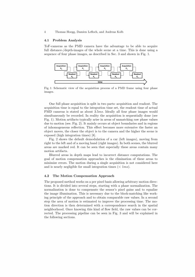
ToF-cameras as the PMD camera have the advantage to be able to acquirefull distance-/depth-images of the whole scene at a time. This is done using asequence of four phase images, as described in Sec. 3 and shown in Fig. 1.

time

Acquisition P0

Readout P0

Acquisition P1

Readout P1

Acquisition P2

Readout P2

Acquisition P3

Readout P3

Fig. 1: Schematic view of the acquisition process of a PMD frame using four phaseimages.

One full phase acquisition is split in two parts: acquisition and readout. Theacquisition time is equal to the integration time set, the readout time of actualPMD cameras is stated as about 3.5ms. Ideally all four phase images wouldsimultaneously be recorded. In reality the acquisition is sequentially done (seeFig. 1). Motion artifacts typically arise in areas of unmatching raw phase valuesdue to motion (see. Fig. 2). It mainly occurs at object boundaries and in regionsof inhomogeneous reflection. This effect becomes more extensive the faster anobject moves, the closer the object is to the camera and the higher the scene isexposed (high integration times) [8].

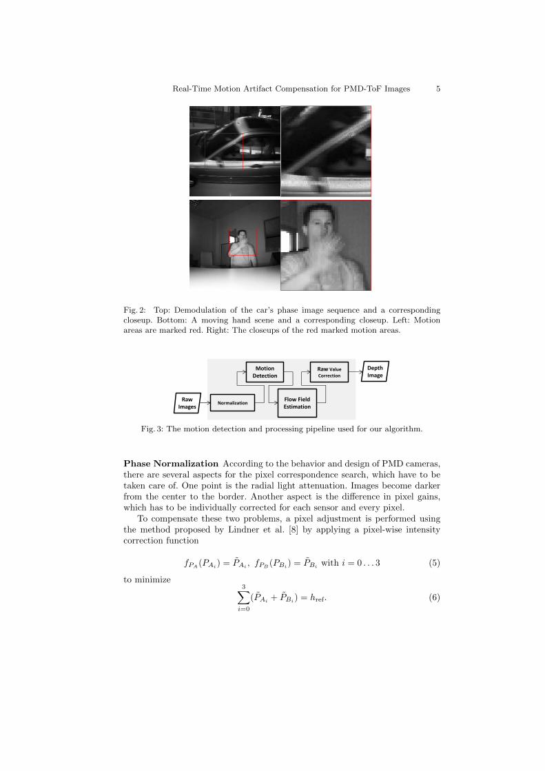
Fig. 2 shows the default demodulation of a car (left images), moving fromright to the left and of a moving hand (right images). In both scenes, the blurredareas are marked red. It can be seen that especially these areas contain manymotion artifacts.

Blurred areas in depth maps lead to incorrect distance computations. Thegoal of motion compensation approaches is the elimination of these areas tominimize errors. The motion during a single acquisition is not considered hereand is nearly negligible for small integration times (< 1ms).

4.2 The Motion Compensation Approach

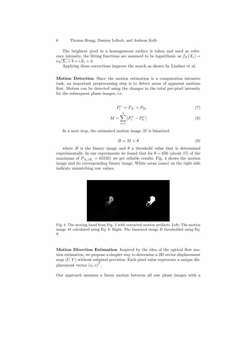
The proposed method works on a per pixel basis allowing arbitrary motion direc-tions. It is divided into several steps, starting with a phase normalization. Thenormalization is done to compensate the sensor’s pixel gains and to equalizethe image illumination. This is necessary due to the block-matching like work-ing principle of the approach and to obtain comparable raw values. In a secondstep the area of motion is estimated to improve the processing time. The mo-tion direction is then determined with a correspondence search in the spatialneighborhood. Once knowing this kind of flow field, the raw values can be cor-rected. The processing pipeline can be seen in Fig. 3 and will be explained inthe following sections.


Fig. 2: Top: Demodulation of the car’s phase image sequence and a correspondingcloseup. Bottom: A moving hand scene and a corresponding closeup. Left: Motionareas are marked red. Right: The closeups of the red marked motion areas.

Raw Images

Normalization

Motion Detection

Flow Field Estimation

Raw Value

Correction

Depth Image

Fig. 3: The motion detection and processing pipeline used for our algorithm.

Phase Normalization According to the behavior and design of PMD cameras,there are several aspects for the pixel correspondence search, which have to betaken care of. One point is the radial light attenuation. Images become darkerfrom the center to the border. Another aspect is the difference in pixel gains,which has to be individually corrected for each sensor and every pixel.

To compensate these two problems, a pixel adjustment is performed usingthe method proposed by Lindner et al. [8] by applying a pixel-wise intensitycorrection function

fPA(PAi) = PAi , fPB

(PBi) = PBi with i = 0 . . . 3 (5)

to minimize3∑

i=0

(PAi+ PBi

) = href. (6)


The brightest pixel in a homogeneous surface is taken and used as refer-ence intensity, the fitting functions are assumed to be logarithmic as fX(Xi) =a√Xi + b+ cXi + d.Applying these corrections improve the search as shown by Lindner et al.

Motion Detection Since the motion estimation is a computation intensivetask, an important preprocessing step is to detect areas of apparent motionsfirst. Motion can be detected using the changes in the total per-pixel intensityfor the subsequent phase images, i.e.

P+i = PAi + PBi (7)

M =

3∑i=1

∣∣P+i − P

+0

∣∣ (8)

In a next step, the estimated motion image M is binarized

B = M > θ (9)

where B is the binary image and θ a threshold value that is determinedexperimentally. In our experiments we found that for θ = 650 (about 1% of themaximum of PAi/Bi

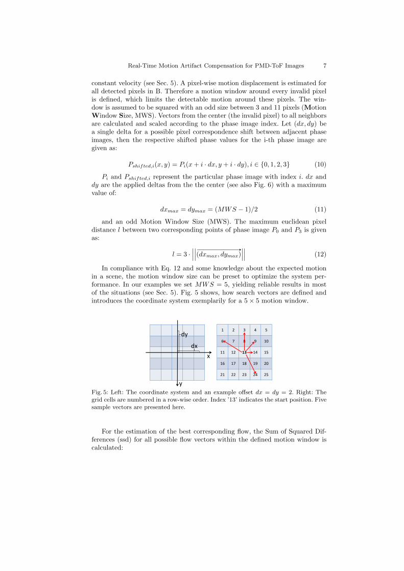
= 65535) we get reliable results. Fig. 4 shows the motionimage and its corresponding binary image. White areas (ones) on the right sideindicate unmatching raw values.

Fig. 4: The moving hand from Fig. 2 with extracted motion artifacts. Left: The motionimage M calculated using Eq. 8. Right: The binarized image B thresholded using Eq.9.

Motion Direction Estimation Inspired by the idea of the optical flow mo-tion estimation, we propose a simpler way to determine a 2D vector displacementmap (U, V ) without subpixel precision. Each pixel value represents a unique dis-

placement vector (u, v)T

.

Our approach assumes a linear motion between all raw phase images with a


constant velocity (see Sec. 5). A pixel-wise motion displacement is estimated forall detected pixels in B. Therefore a motion window around every invalid pixelis defined, which limits the detectable motion around these pixels. The win-dow is assumed to be squared with an odd size between 3 and 11 pixels (MotionWindow Size, MWS). Vectors from the center (the invalid pixel) to all neighborsare calculated and scaled according to the phase image index. Let (dx, dy) bea single delta for a possible pixel correspondence shift between adjacent phaseimages, then the respective shifted phase values for the i-th phase image aregiven as:

Pshifted,i(x, y) = Pi(x+ i · dx, y + i · dy), i ∈ {0, 1, 2, 3} (10)

Pi and Pshifted,i represent the particular phase image with index i. dx anddy are the applied deltas from the the center (see also Fig. 6) with a maximumvalue of:

dxmax = dymax = (MWS − 1)/2 (11)

and an odd Motion Window Size (MWS). The maximum euclidean pixeldistance l between two corresponding points of phase image P0 and P3 is givenas:

l = 3 ·∣∣∣∣∣∣ # »

(dxmax, dymax)∣∣∣∣∣∣ (12)

In compliance with Eq. 12 and some knowledge about the expected motionin a scene, the motion window size can be preset to optimize the system per-formance. In our examples we set MWS = 5, yielding reliable results in mostof the situations (see Sec. 5). Fig. 5 shows, how search vectors are defined andintroduces the coordinate system exemplarily for a 5× 5 motion window.

1 2 3 4 5

6 7 8 9 10

11 12 13 14 15

16 17 18 19 20

21 22 23 24 25

x

dx

dy

y

Fig. 5: Left: The coordinate system and an example offset dx = dy = 2. Right: Thegrid cells are numbered in a row-wise order. Index ’13’ indicates the start position. Fivesample vectors are presented here.

For the estimation of the best corresponding flow, the Sum of Squared Dif-ferences (ssd) for all possible flow vectors within the defined motion window iscalculated:


1 2 3 4 5

6 7 8 9 10

11 12 13 14 15 … …

16 17 18 19 20

21 22 23 24 25

P1 P2 P3 P4

dx 2dx 3dx dy 2dy 3dy

dx=1 dy=0

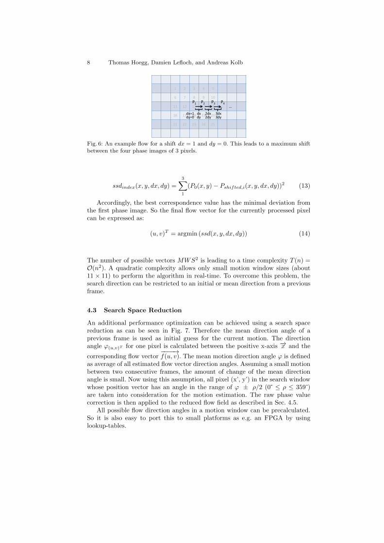
Fig. 6: An example flow for a shift dx = 1 and dy = 0. This leads to a maximum shiftbetween the four phase images of 3 pixels.

ssdindex(x, y, dx, dy) =

3∑1

(P0(x, y)− Pshifted,i(x, y, dx, dy))2 (13)

Accordingly, the best correspondence value has the minimal deviation fromthe first phase image. So the final flow vector for the currently processed pixelcan be expressed as:

(u, v)T = argmin (ssd(x, y, dx, dy)) (14)

The number of possible vectors MWS2 is leading to a time complexity T (n) =O(n2). A quadratic complexity allows only small motion window sizes (about11 × 11) to perform the algorithm in real-time. To overcome this problem, thesearch direction can be restricted to an initial or mean direction from a previousframe.

4.3 Search Space Reduction

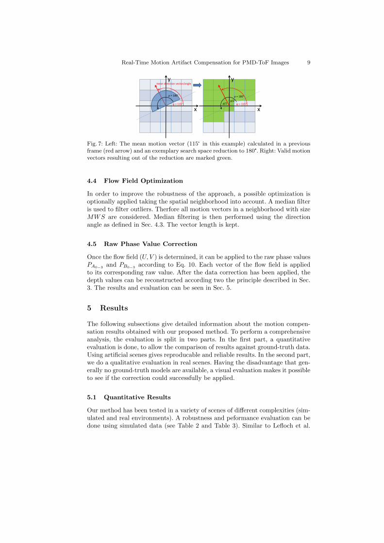
An additional performance optimization can be achieved using a search spacereduction as can be seen in Fig. 7. Therefore the mean direction angle of aprevious frame is used as initial guess for the current motion. The directionangle ϕ(u,v)T for one pixel is calculated between the positive x-axis −→x and the

corresponding flow vector−−−−→f(u, v). The mean motion direction angle ϕ is defined

as average of all estimated flow vector direction angles. Assuming a small motionbetween two consecutive frames, the amount of change of the mean directionangle is small. Now using this assumption, all pixel (x’, y’) in the search windowwhose position vector has an angle in the range of ϕ ± ρ/2 (0° ≤ ρ ≤ 359°)are taken into consideration for the motion estimation. The raw phase valuecorrection is then applied to the reduced flow field as described in Sec. 4.5.

All possible flow direction angles in a motion window can be precalculated.So it is also easy to port this to small platforms as e.g. an FPGA by usinglookup-tables.


x

y

ρ = 180°

x

y

ρ = 180°

mean direction vector/angle

ϕ = 115° ρ/2 ρ/2

ϕ = 115°

Fig. 7: Left: The mean motion vector (115° in this example) calculated in a previousframe (red arrow) and an exemplary search space reduction to 180°. Right: Valid motionvectors resulting out of the reduction are marked green.

4.4 Flow Field Optimization

In order to improve the robustness of the approach, a possible optimization isoptionally applied taking the spatial neighborhood into account. A median filteris used to filter outliers. Therfore all motion vectors in a neighborhood with sizeMWS are considered. Median filtering is then performed using the directionangle as defined in Sec. 4.3. The vector length is kept.

4.5 Raw Phase Value Correction

Once the flow field (U, V ) is determined, it can be applied to the raw phase valuesPA0−3 and PB0−3 according to Eq. 10. Each vector of the flow field is appliedto its corresponding raw value. After the data correction has been applied, thedepth values can be reconstructed according two the principle described in Sec.3. The results and evaluation can be seen in Sec. 5.

5 Results

The following subsections give detailed information about the motion compen-sation results obtained with our proposed method. To perform a comprehensiveanalysis, the evaluation is split in two parts. In the first part, a quantitativeevaluation is done, to allow the comparison of results against ground-truth data.Using artificial scenes gives reproducable and reliable results. In the second part,we do a qualitative evaluation in real scenes. Having the disadvantage that gen-erally no ground-truth models are available, a visual evaluation makes it possibleto see if the correction could successfully be applied.

5.1 Quantitative Results

Our method has been tested in a variety of scenes of different complexities (sim-ulated and real environments). A robustness and peformance evaluation can bedone using simulated data (see Table 2 and Table 3). Similar to Lefloch et al.


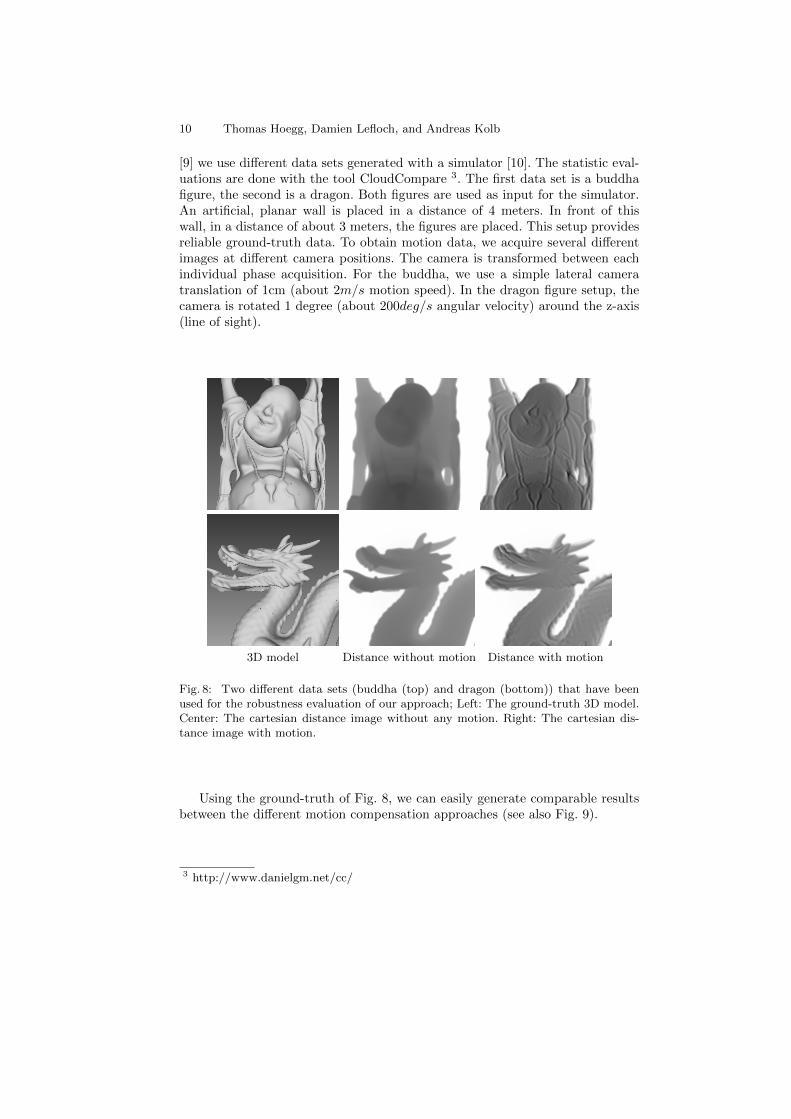
[9] we use different data sets generated with a simulator [10]. The statistic eval-uations are done with the tool CloudCompare 3. The first data set is a buddhafigure, the second is a dragon. Both figures are used as input for the simulator.An artificial, planar wall is placed in a distance of 4 meters. In front of thiswall, in a distance of about 3 meters, the figures are placed. This setup providesreliable ground-truth data. To obtain motion data, we acquire several differentimages at different camera positions. The camera is transformed between eachindividual phase acquisition. For the buddha, we use a simple lateral cameratranslation of 1cm (about 2m/s motion speed). In the dragon figure setup, thecamera is rotated 1 degree (about 200deg/s angular velocity) around the z-axis(line of sight).

3D model Distance without motion Distance with motion

Fig. 8: Two different data sets (buddha (top) and dragon (bottom)) that have beenused for the robustness evaluation of our approach; Left: The ground-truth 3D model.Center: The cartesian distance image without any motion. Right: The cartesian dis-tance image with motion.

Using the ground-truth of Fig. 8, we can easily generate comparable resultsbetween the different motion compensation approaches (see also Fig. 9).

3 http://www.danielgm.net/cc/


Proposed method Lindner et al. Lefloch et al.

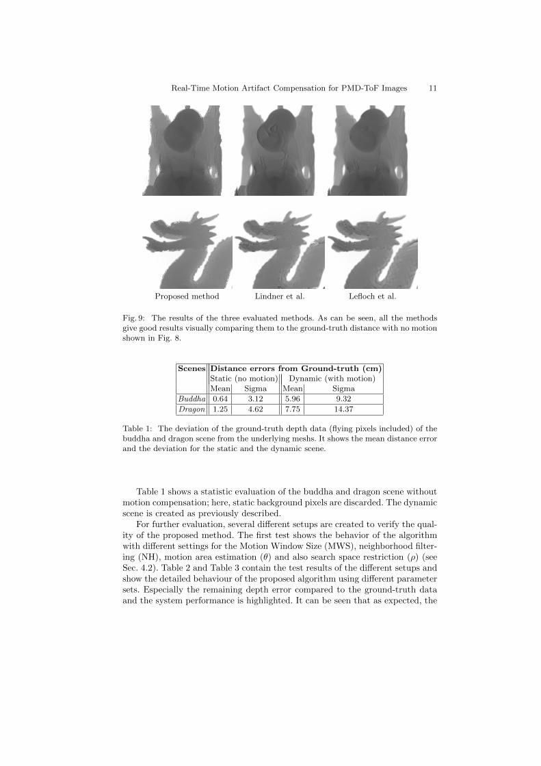
Fig. 9: The results of the three evaluated methods. As can be seen, all the methodsgive good results visually comparing them to the ground-truth distance with no motionshown in Fig. 8.

Scenes Distance errors from Ground-truth (cm)Static (no motion) Dynamic (with motion)Mean Sigma Mean Sigma

Buddha 0.64 3.12 5.96 9.32

Dragon 1.25 4.62 7.75 14.37

Table 1: The deviation of the ground-truth depth data (flying pixels included) of thebuddha and dragon scene from the underlying meshs. It shows the mean distance errorand the deviation for the static and the dynamic scene.

Table 1 shows a statistic evaluation of the buddha and dragon scene withoutmotion compensation; here, static background pixels are discarded. The dynamicscene is created as previously described.

For further evaluation, several different setups are created to verify the qual-ity of the proposed method. The first test shows the behavior of the algorithmwith different settings for the Motion Window Size (MWS), neighborhood filter-ing (NH), motion area estimation (θ) and also search space restriction (ρ) (seeSec. 4.2). Table 2 and Table 3 contain the test results of the different setups andshow the detailed behaviour of the proposed algorithm using different parametersets. Especially the remaining depth error compared to the ground-truth dataand the system performance is highlighted. It can be seen that as expected, the


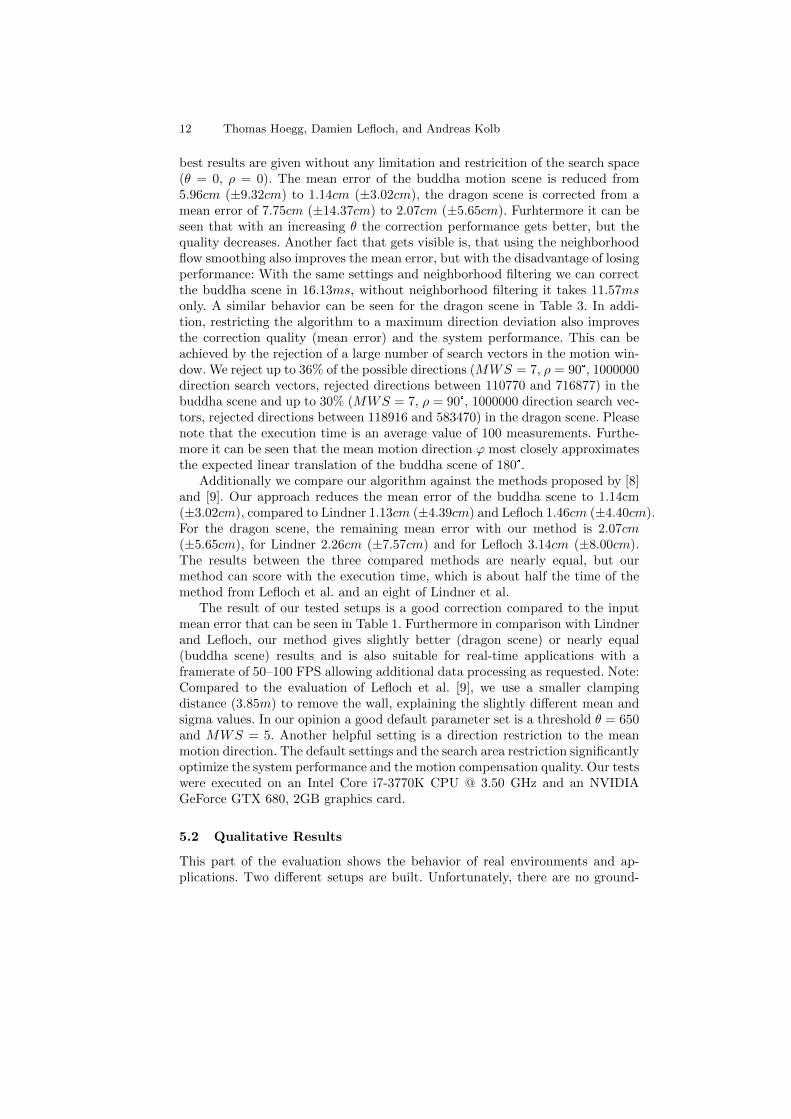
best results are given without any limitation and restricition of the search space(θ = 0, ρ = 0). The mean error of the buddha motion scene is reduced from5.96cm (±9.32cm) to 1.14cm (±3.02cm), the dragon scene is corrected from amean error of 7.75cm (±14.37cm) to 2.07cm (±5.65cm). Furhtermore it can beseen that with an increasing θ the correction performance gets better, but thequality decreases. Another fact that gets visible is, that using the neighborhoodflow smoothing also improves the mean error, but with the disadvantage of losingperformance: With the same settings and neighborhood filtering we can correctthe buddha scene in 16.13ms, without neighborhood filtering it takes 11.57msonly. A similar behavior can be seen for the dragon scene in Table 3. In addi-tion, restricting the algorithm to a maximum direction deviation also improvesthe correction quality (mean error) and the system performance. This can beachieved by the rejection of a large number of search vectors in the motion win-dow. We reject up to 36% of the possible directions (MWS = 7, ρ = 90°, 1000000direction search vectors, rejected directions between 110770 and 716877) in thebuddha scene and up to 30% (MWS = 7, ρ = 90°, 1000000 direction search vec-tors, rejected directions between 118916 and 583470) in the dragon scene. Pleasenote that the execution time is an average value of 100 measurements. Furthe-more it can be seen that the mean motion direction ϕ most closely approximatesthe expected linear translation of the buddha scene of 180°.

Additionally we compare our algorithm against the methods proposed by [8]and [9]. Our approach reduces the mean error of the buddha scene to 1.14cm(±3.02cm), compared to Lindner 1.13cm (±4.39cm) and Lefloch 1.46cm (±4.40cm).For the dragon scene, the remaining mean error with our method is 2.07cm(±5.65cm), for Lindner 2.26cm (±7.57cm) and for Lefloch 3.14cm (±8.00cm).The results between the three compared methods are nearly equal, but ourmethod can score with the execution time, which is about half the time of themethod from Lefloch et al. and an eight of Lindner et al.

The result of our tested setups is a good correction compared to the inputmean error that can be seen in Table 1. Furthermore in comparison with Lindnerand Lefloch, our method gives slightly better (dragon scene) or nearly equal(buddha scene) results and is also suitable for real-time applications with aframerate of 50–100 FPS allowing additional data processing as requested. Note:Compared to the evaluation of Lefloch et al. [9], we use a smaller clampingdistance (3.85m) to remove the wall, explaining the slightly different mean andsigma values. In our opinion a good default parameter set is a threshold θ = 650and MWS = 5. Another helpful setting is a direction restriction to the meanmotion direction. The default settings and the search area restriction significantlyoptimize the system performance and the motion compensation quality. Our testswere executed on an Intel Core i7-3770K CPU @ 3.50 GHz and an NVIDIAGeForce GTX 680, 2GB graphics card.

5.2 Qualitative Results

This part of the evaluation shows the behavior of real environments and ap-plications. Two different setups are built. Unfortunately, there are no ground-


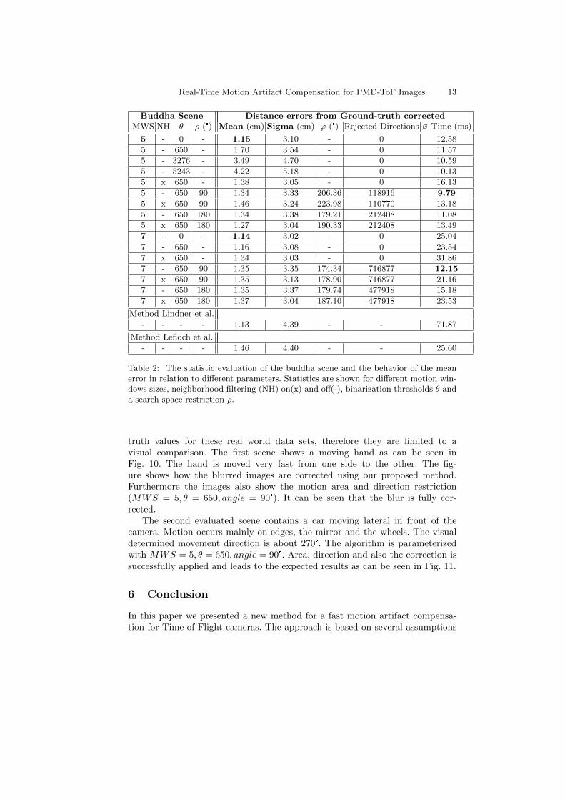
Buddha Scene Distance errors from Ground-truth correctedMWS NH θ ρ (°) Mean (cm) Sigma (cm) ϕ (°) Rejected Directions � Time (ms)

5 - 0 - 1.15 3.10 - 0 12.58

5 - 650 - 1.70 3.54 - 0 11.57

5 - 3276 - 3.49 4.70 - 0 10.59

5 - 5243 - 4.22 5.18 - 0 10.13

5 x 650 - 1.38 3.05 - 0 16.13

5 - 650 90 1.34 3.33 206.36 118916 9.79

5 x 650 90 1.46 3.24 223.98 110770 13.18

5 - 650 180 1.34 3.38 179.21 212408 11.08

5 x 650 180 1.27 3.04 190.33 212408 13.49

7 - 0 - 1.14 3.02 - 0 25.04

7 - 650 - 1.16 3.08 - 0 23.54

7 x 650 - 1.34 3.03 - 0 31.86

7 - 650 90 1.35 3.35 174.34 716877 12.15

7 x 650 90 1.35 3.13 178.90 716877 21.16

7 - 650 180 1.35 3.37 179.74 477918 15.18

7 x 650 180 1.37 3.04 187.10 477918 23.53

Method Lindner et al.

- - - - 1.13 4.39 - - 71.87

Method Lefloch et al.

- - - - 1.46 4.40 - - 25.60

Table 2: The statistic evaluation of the buddha scene and the behavior of the meanerror in relation to different parameters. Statistics are shown for different motion win-dows sizes, neighborhood filtering (NH) on(x) and off(-), binarization thresholds θ anda search space restriction ρ.

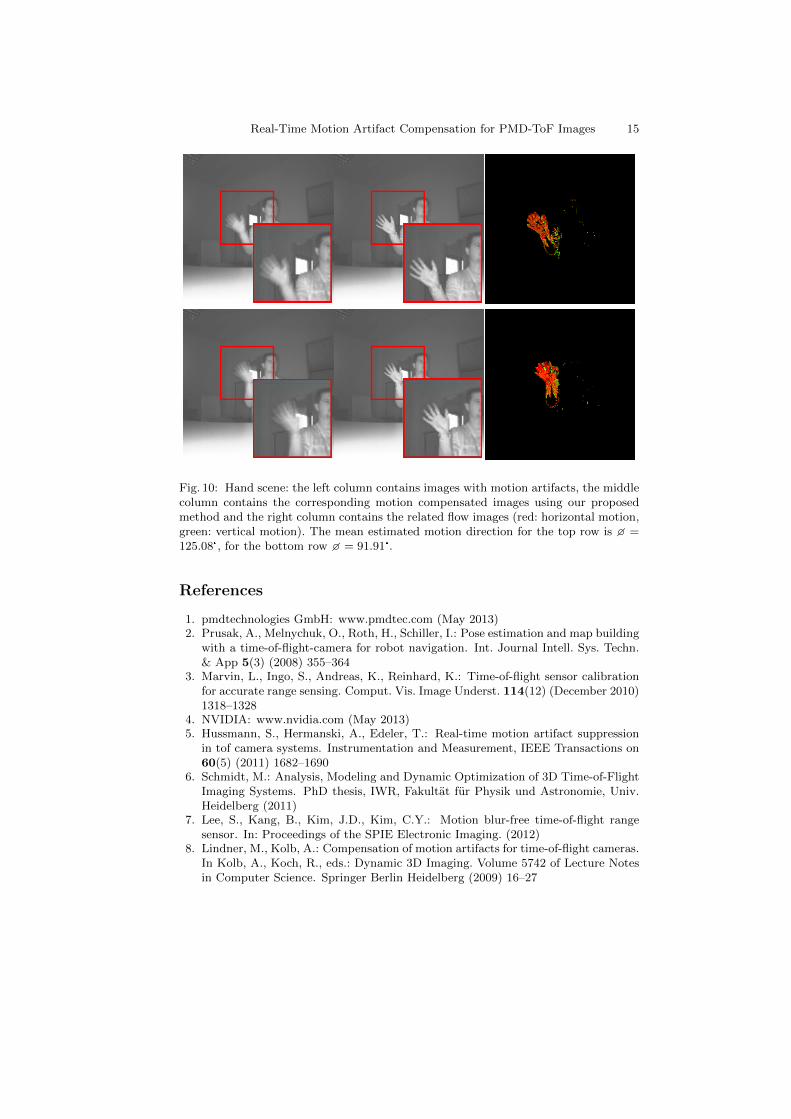
truth values for these real world data sets, therefore they are limited to avisual comparison. The first scene shows a moving hand as can be seen inFig. 10. The hand is moved very fast from one side to the other. The fig-ure shows how the blurred images are corrected using our proposed method.Furthermore the images also show the motion area and direction restriction(MWS = 5, θ = 650, angle = 90°). It can be seen that the blur is fully cor-rected.

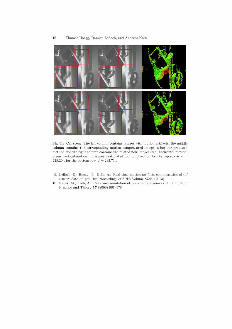
The second evaluated scene contains a car moving lateral in front of thecamera. Motion occurs mainly on edges, the mirror and the wheels. The visualdetermined movement direction is about 270°. The algorithm is parameterizedwith MWS = 5, θ = 650, angle = 90°. Area, direction and also the correction issuccessfully applied and leads to the expected results as can be seen in Fig. 11.

6 Conclusion

In this paper we presented a new method for a fast motion artifact compensa-tion for Time-of-Flight cameras. The approach is based on several assumptions


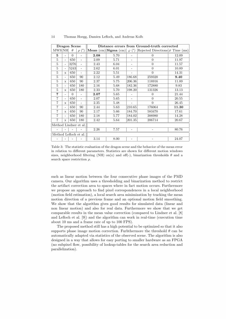
Dragon Scene Distance errors from Ground-truth correctedMWS NH θ ρ (°) Mean (cm) Sigma (cm) ϕ (°) Rejected Directions � Time (ms)

5 - 0 - 2.08 5.70 - 0 12.09

5 - 650 - 2.09 5.71 - 0 11.97

5 - 3276 - 2.43 6.04 - 0 11.57

5 - 5243 - 2.62 6.01 - 0 10.89

5 x 650 - 2.22 5.51 - 0 14.31

5 - 650 90 2.12 5.49 186.68 259320 9.40

5 x 650 90 2.37 5.75 206.36 118916 11.89

5 - 650 180 2.16 5.68 182.36 172880 9.83

5 x 650 180 2.33 5.70 198.20 131326 13.13

7 - 0 - 2.07 5.65 - 0 21.44

7 - 650 - 2.07 5.65 - 0 20.55

7 x 650 - 2.35 5.48 - 0 26.45

7 - 650 90 2.44 5.63 210.65 176064 11.30

7 x 650 90 2.17 5.66 184.70 583470 17.61

7 - 650 180 2.18 5.77 184.02 388980 14.28

7 x 650 180 2.42 5.64 201.35 206714 20.67

Method Lindner et al.

- - - - 2.26 7.57 - - 80.76

Method Lefloch et al.

- - - - 3.14 8.00 - - 24.07

Table 3: The statistic evaluation of the dragon scene and the behavior of the mean errorin relation to different parameters. Statistics are shown for different motion windowssizes, neighborhood filtering (NH) on(x) and off(-), binarization thresholds θ and asearch space restriction ρ.

such as linear motion between the four consecutive phase images of the PMDcamera. Our algorithm uses a thresholding and binarization method to restrictthe artifact correction area to spaces where in fact motion occurs. Furthermorewe propose an approach to find pixel correspondences in a local neighborhood(motion field estimation), a local search area minimization by tracking the meanmotion direction of a previous frame and an optional motion field smoothing.We show that the algorithm gives good results for simulated data (linear andnon linear motion) and also for real data. Furthermore we show that we getcomparable results in the mean value correction (compared to Lindner et al. [8]and Lefloch et al. [9]) and the algorithm can work in real-time (execution timeabout 10 ms and a frame rate of up to 100 FPS).

The proposed method still has a high potential to be optimized so that it alsosupports phase image motion correction. Furhthermore the threshold θ can beautomatically adapted via statistics of the observed scene. The algorithm is alsodesigned in a way that allows for easy porting to smaller hardware as an FPGA(no subpixel flow, possibility of lookup-tables for the search area reduction andparallelization).


Fig. 10: Hand scene: the left column contains images with motion artifacts, the middlecolumn contains the corresponding motion compensated images using our proposedmethod and the right column contains the related flow images (red: horizontal motion,green: vertical motion). The mean estimated motion direction for the top row is � =125.08°, for the bottom row � = 91.91°.

References

1. pmdtechnologies GmbH: www.pmdtec.com (May 2013)2. Prusak, A., Melnychuk, O., Roth, H., Schiller, I.: Pose estimation and map building

with a time-of-flight-camera for robot navigation. Int. Journal Intell. Sys. Techn.& App 5(3) (2008) 355–364

3. Marvin, L., Ingo, S., Andreas, K., Reinhard, K.: Time-of-flight sensor calibrationfor accurate range sensing. Comput. Vis. Image Underst. 114(12) (December 2010)1318–1328

4. NVIDIA: www.nvidia.com (May 2013)5. Hussmann, S., Hermanski, A., Edeler, T.: Real-time motion artifact suppression

in tof camera systems. Instrumentation and Measurement, IEEE Transactions on60(5) (2011) 1682–1690

6. Schmidt, M.: Analysis, Modeling and Dynamic Optimization of 3D Time-of-FlightImaging Systems. PhD thesis, IWR, Fakultat fur Physik und Astronomie, Univ.Heidelberg (2011)

7. Lee, S., Kang, B., Kim, J.D., Kim, C.Y.: Motion blur-free time-of-flight rangesensor. In: Proceedings of the SPIE Electronic Imaging. (2012)

8. Lindner, M., Kolb, A.: Compensation of motion artifacts for time-of-flight cameras.In Kolb, A., Koch, R., eds.: Dynamic 3D Imaging. Volume 5742 of Lecture Notesin Computer Science. Springer Berlin Heidelberg (2009) 16–27


Fig. 11: Car scene: The left column contains images with motion artifacts, the middlecolumn contains the corresponding motion compensated images using our proposedmethod and the right column contains the related flow images (red: horizontal motion,green: vertical motion). The mean estimated motion direction for the top row is � =228.20°, for the bottom row � = 232.71°.

9. Lefloch, D., Hoegg, T., Kolb, A.: Real-time motion artifacts compensation of tofsensors data on gpu. In: Proceedings of SPIE Volume 8738. (2013)

10. Keller, M., Kolb, A.: Real-time simulation of time-of-flight sensors. J. SimulationPractice and Theory 17 (2009) 967–978

Documents

Real-Time Motion Artifact Compensation for PMD-ToF … · Real-Time Motion Artifact Compensation for PMD-ToF Images Thomas Hoegg1, Damien Le och 2, and Andreas Kolb ... standard methods