Receiver Noise Temperature, the Quantum Noise Limit, and ... · the noise power per unit bandwidth. The noise temperature of a black body radiator at physical temperature T is obtained

Eighth International Symposium on Space Terahertz Technology, Harvard University, March 1997

Receiver Noise Temperature, the Quantum Noise Limit, andthe Role of the Zero-Point Fluctuations*

A. R. Kerr', M. J. Feldman 2 and S.-K. Panl

1National Radio Astronomy Observatory**Charlottesville, VA 22903

2Department of Electrical EngineeringUniversity of RochesterRochester, NY 14627

Abstract

There are in use at present three different ways of deducing the receivernoise temperature TR from the measured Y-factor, each resulting in a differentvalue of TR . The methods differ in the way the physical temperatures of the hotand cold loads, Th and Tc (usually room temperature and liquid nitrogen), areconverted into radiated power "temperatures" to deduce T R from Y. Only one ofthese methods is consistent with Tucker's quantum mixer theory and theconstraints of Heisenberg's uncertainty principle. The paper also examines theminimum system noise temperatures achievable with single- and double-sidebandreceivers.

Introduction

After talking to people at the 1996 Symposium on Space TerahertzTechnology, it was clear that there was some confusion, or at least differenceof opinion, on how to deduce the noise temperature of a receiver from themeasured Y-factor. There was also disagreement on the fundamental quantum noiselimit of single- and double-sideband mixer receivers. With the (DSB) noisetemperatures of the best SIS receivers now approaching 2hf/k (-30 K at 300 GHz),these questions need to be resolved. This paper compares the threeinterpretations of the Y-factor measurement currently in use, and discusses thefundamental quantum limit on the sensitivity of coherent receivers.

The Y-factor Method

In a Y-factor measurement, two noise sources are connected individually tothe receiver input, and the ratio, Y, of the receiver output powers is measured.From the Y-factor the intrinsic noise of the receiver can be deduced, either asan equivalent input noise power or as an equivalent input noise temperature.While noise temperatures are most commonly used, the discussion will be clearerif we consider noise powers initially.

* Originally printed as Electronics Division Internal Report No. 304, National Radio Astronomy Observatory,Charlottesville VA 22903, September 1996.

** The National Radio Astronomy Observatory is a facility of the National Science Foundation operated undercooperative agreement by Associated Universities, Inc.

101


Let Pn be the equivalent input noise power of the receiver in a bandwidthB, the measurement bandwidth. B is defined by a bandpass filter at the receiveroutput (for a coherent receiver (e.g., amplifier or mixer) an input filter isunnecessary) . With a power Pin incident on the receiver in bandwidth B, the

measured output power of the receiver P mit = G[P n + P 1 ], where G is the gain ofthe receiver. With hot and cold loads in front of the receiver the measured Y-factor is:

p n phot

Y

Pn Pcold

The equivalent input noise power is found by inverting this equation:

p n _ Phot Y P cold

Y - 1

Frequently the hot and cold loads are simply black-body radiators (well matchedwaveguide or free-space loads) heated or cooled to accurately known physicaltemperatures Thot and Tcoid.

Power Radiated by a Black Body

The Planck radiation law is often used to calculate the thermal noise powerin a bandwidth B about frequency f (B << f), radiated into a single mode (e.g.,a waveguide mode), by a black body at physical temperature T:

(1)

(2)

hf

kT

hfiexp-. -1kT

p Planck = kTB (3)

where, h and k are the Planck and Boltzmann constants. In the present context,a more complete description is given by the dissipation-fluctuation theorem, orgeneralized Nyquist theorem, of Callen & Welton NJ:

hf

kT

expl.hfi -1kT

P C&W = kTBhfB

2(4)

hfB coth(i?-_)

This is simply the Planck formula with an additional half photon per Hz, hfB/2,

2 t 2kT

1 02

(5)-1exp

hfkThfkT

(6)2k 2k 2kT

hfkThfkT

exp=•■■••• CO L.11 •

hf , u( hf)hfT c'w = T


and it is this additional half photon, the zero-point fluctuation noise, that isthe source of some confusion. Some authors believe that the zero-pointfluctuations should be excluded from consideration of noise powers because theydo not represent exchangeable power. However, the view of Devyatov et al. [2]is that, although the zero-point fluctuations deliver no real power, the receivernevertheless "...develops these quantum fluctuations to quite measurablefluctuations..." at its output. The zero-point fluctuations, they argue, shouldbe associated with the incoming radiation and not with the receiver itself: atthe receiver input "...one can imagine two zero-point fluctuation wavespropagating in opposite directions..." with no net power flow.

It is interesting to note [3] that in the limit of small hf/kT, it is theCallen and Welton formula (4) which gives the Rayleigh-Jeans result P = kTB,while the Planck formula (3) gives P = kTB hfB/2, half a photon below theRayleigh-Jeans result.

Noise Temperatures

The noise power Pn in a bandwidth B is conveniently represented by a noisetemperature Tn = Pn/kB. The noise temperature is simply a shorthand notation forthe noise power per unit bandwidth. The noise temperature of a black bodyradiator at physical temperature T is obtained from the noise power (3, 4) as:

T " T

These expressions differ by the zero-point fluctuation noise temperature, hf/2k,whose magnitude is 0.024 K per GHz. In the Rayleigh-Jeans limit of small hf/kT,the noise temperature based on the Callen & Welton formula approaches thephysical temperature of the black body ( Tc6'/1 -.0 T), while the noise temperaturebased on the Planck formula is half a photon below the physical temperature( TPlanck -4 T hf/2k). Fig. 1 shows Tn evaluated according to (5) and (6), asfunctions of the physical temperature T of the black body, for a frequency of 230

Planck,GHz. Also shown are the differences between T TC&W, and TRJ.

1 03

f = 230

1

GHz

T(planck)

T(C&W) -

/

T(Planck)

T(C&W)

_____

T(R-J)

\\\\

,..--.

__------

--------

- -

T(C&W)

1-

T(phys) - T(Planck)

- T(phys)

..........---

I,

20

15

=

010

0

5

0-


0 5 10 15 20Physical Temperature K

Fig.l. Noise temperature vs physical temperature for black body radiators at 230 GHz, according to the Rayleigh-Jeans, Planck, and Callen & Welton laws. Also shown (broken lines) are the differences between the threeradiation curves. The Rayleigh-Jeans curve converges to the Callen & Welton curve at high temperature, whilethe Planck curve is always hf/2k below the Callen & Welton curve.

Receiver noise temperature from the Y-factor

Equation (2) for the equivalent input noise power of a receiver can bewritten in terms of noise temperatures using Tn = Pn/kB. Thus the equivalentinput noise temperature l of the receiver,

n _ Tnhot Tncold

Y- 1

Three different interpretations of this equation are in use at present. Theydiffer in the values of T;,', and TL id assumed for the hot and cold loads atphysical temperatures Thot and T coid . Most often, the Rayleigh-Jeans formula is

1 This definition of receiver noise temperature is now generally accepted in the millimeter and submillimeter receivercommunity. There are two older definitions of receiver noise temperature which are based on hypotheticalmeasurements rather than on the simple Y-factor measurement (i) The physical temperature of the input termination ofa hypothetical noise-free device, which would resutt in the same output noise power as the actual device connected to anoise-free input termination. (ii) The physical temperature of the input termination required to double the output noise ofthe same receiver with its input termination at absolute zero temperature. Using either of these older definitions causesfurther complications, beyond the scope of this paper. This question was dealt with at length in [5].

(7)

104


used, in which T IL and TLid are equal to the physical temperatures. Someworkers use the Planck formula (5), while others use the Callen & Welton formula(6). The three approaches result in three different values of TR

n , which we11RJ , TRPlanck,denote T and TRC&W:

RJ Thot Tcold TR — (8)

Y - 1

Planck PlanckPlanck _

T hot

Y T cold

TR

andC&W col

T CCM _ Thot

Y T cold

Y - 1

It will become clear in the following sections that only eq.(10) gives a receivernoise temperature consistent with quantum mixer theory [4] and the constraintsof the uncertainty principle.

For a given value of Y, the difference between the Planck and Callen &Welton formulas (9, 10) is just half a photon:

Planck_ hfTR T

R 2k

This constant half photon difference is independent of the hot and cold loadtemperatures. The difference between the Rayleigh-Jeans and Callen & Weltonformulas (8, 10) depends on the physical temperatures of the hot and cold loads,and on frequency. Fig. 2 shows the receiver noise temperature, calculatedaccording to eqs. (8-10), as a function of Y-factor for a 230 GHz receiver,measured with hot and cold loads at physical temperatures 300 K and 77 K. Thesmall difference between the Rayleigh-Jeans and Callen & Welton results is shownby the dashed curve and referred to the right-hand scale. The negative receivernoise temperatures correspond to physically impossible values of the Y-factor.The physical limits on TR

n will be discussed below.

The difference between receiver noise temperatures obtained using theRayleigh-Jeans and Callen & Welton laws is not always as small as in the examplein Fig. 2. Only if hf/kT << 1 for the hot and cold loads will T;L7 Z

T RC&W . For

example, if a 230 GHz receiver were measured using 4 K and room temperatureloads, hf/ kTcoid = 2.8, and T;

47 is -2.3 K larger than T RC&W . Another example is

an 800 GHz receiver measured using 77 K and roam temperature loads; then hf/kT„id= 0.5, and T;"-7 would be -2.0 K larger than TR"w.

So far there has been no mention of single- or double-sideband operation.That is because the above discussion applies to both SSB and DSB receivers; a Y-factor measurement on a SSB or DSB receiver gives, via equation (7), the SSB orDSB receiver noise temperature.

Y-(9)

(10)

105

3.20 3.40 3.60 3.80Y-factor

4.00 4.20 4.40


Fig. 2. Receiver noise temperature as a function of Y-factor for a 230 GHz receiver measured with T hot = 300 Kand T = • 7 K The Rayleigh-Jeans curve is obtained when the hot and cold load noise temperatures are equalto their physical temperatures. The Planck and Callen & Welton curves are obtained using equations (5) and(6)for the hot and cold load noise temperatures. The small difference between the Planck and Callen & Weltoncurves is indicated by the dashed line (right-hand scale).

Single- and Double- Sideband Mixer Receivers

Mixer receivers can operate in several modes, depending on theconfiguration of the receiver and the nature of the measurement. In single-sideband operation, the receiver is configured so that, at the image sideband,the mixer is connected to a termination within the receiver. There is noexternal connection to the image frequency, and the complete receiver isfunctionally equivalent to an amplifier followed by a frequency converter. Indouble-sideband operation, on the other hand, the mixer is connected to the sameinput port at both upper and lower sidebands. A DSB receiver can be used in twomodes: (i) to measure narrow-band signals contained entirely within one sideband- this is SSB operation of a DSB receiver. For detection of such narrow-bandSignals, power collected in the image band of a DSB receiver degrades themeasurement sensitivity. And (ii), to measure broadband (or continuum) sourceswhose spectrum covers both sidebands - this is DSB operation of a DSB receiver.For continuum radiometry, the additional signal power collected in the image bandof a DSB receiver imlaroves the measurement sensitivity.

A 7-'actor measurement on a DSB receiver, interpreted according to eq. (7),gives the so-called DSB receiver noise temperature. This is the most commonlyo7ucted noise temperature for mixer receivers because it is easy to measure. Itis also common to derive a SSB noise temperature (for a DSB receiver) bymeasuring the sideband gains, and referring all the receiver noise to a single

106

G.

Gs( (13)

Pout

kBGsT T + TR

n, SSBTsnys,,SSB


sideband, the signal sideband. Then, for the DSB receiver,

TRn, SS13 nTR,DSB

where Gs and Gi are the receiver gains at the signal and image frequencies2,measured from the hot/cold load input port. If the upper and lower sideband

gains are equal, TRn, SSB = 2

TRn,DSB If Gi << Gs , the Y-factor measurement directly

gives TRn, SSB ' When a DSB mixer receiver is used to receive a narrow-band signal

contained entirely within one sideband, noise from the image band contributes tothe output of the receiver. The overall SSE system noise temperature

G.1 +

Gs.

(12)

G. 1= T s

n + T TRn, DSB 1

+1 Gs

where T: and Ti:r1 are the noise temperatures of the signal and image terminations.

Fundamental Limits on TR

The fundamental limits imposed by the Heisenberg uncertainty principle onthe noise of amplifiers, parametric amplifiers, and mixer receivers have beenstudied by a number of authors over the last thirty five years, and their workis reviewed, with particular attention to mixer receivers, in [5] and [6]. Thefollowing general statement can be made: The minimum output noise power of ameasurement system using a mixer receiver, SSB or DSB, is hf (i.e. one photon)per unit bandwidth, referred to one sideband at the receiver input. Hence, theminimum system noise temperature is hf/k referred to one sideband at the receiverinput — exactly the same result as for a system incorporating an amplifier. Theorigin of this quantum noise has been much discussed [7, 3, 5, 6], and will beexplained with the aid of Figs. 3 and 4, which depict four minimum-noisemeasurement systems using mixer receivers.

Fig. 3 shows two SSB receivers, 3(a) with a short-circuited image, and 3(b)with an image-frequency termination equal to the signal source resistance. Forboth 3(a) and 3(b), Tucker's quantum mixer theory predicts [4, 5, 8] a minimumreceiver noise temperature of hf/2k. In 3(a) the zero-point fluctuationsassociated with the input termination (at 0 K) contribute half a photon (hf/2k)to the overall system noise temperature, and the mixer contributes the remaining

2 For simplicity, we assume there is no significant conversion of higher harmonic sideband signals present at theinput port. If the receiver gain is not negligible at frequencies nf Lo ± n > 1, then additional terms of the form Gn/G,must be added in the parentheses on the right side of eq. (12).

G.

Gs

107


half photon , which can be shown to originate in the electron shot noise in themixer. In (b), the zero-point fluctuations associated with the signal source and(internal) image termination each contribute half a photon, which accounts forall the system noise; the mixer itself contributes no noise, which is exactly theresult obtained from mixer theory. Here, the down-converted components of themixer shot noise exactly cancel the IF component, with which they are correlated,a result well known in classical mixer theory.

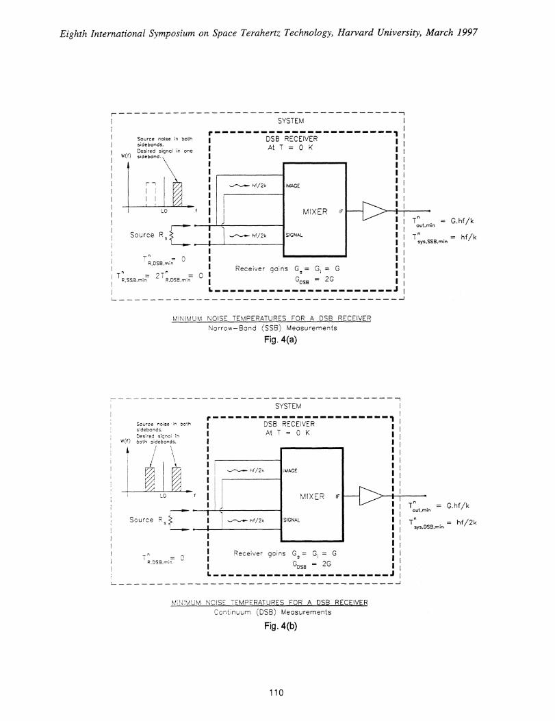
Fig. 4 shows a DSB mixer receiver used in two different measurement modes:4(a) to measure a signal present only in one sideband (the SSB mode for a DSBreceiver), and 4(b) to measure a broadband signal present in both sidebands (theDSB or continuum mode). In 4(a), zero-point fluctuations associated with theinput termination (at 0 K) contribute half a photon (hf/2k) in each sideband,and the mixer need contribute no noise, consistent with mixer theory. The sameis true in 4(b), in which the presence of the signal in both sidebands doublesthe signal power at the output of the system, and the signal-to-noise ratio atthe output is twice that of the SSB receivers in Fig. 3. It is this apparentdoubling of the receiver gain that leads to the concept of the DSB gain, GDsB =2G (provided the signal and image gains are equal, i.e., Gs = Gi = G).

It is clear from Figs. 3 and 4 that the minimum receiver noise temperaturesfor SSE and DSB receivers are, respectively, hf/2k and zero. The minimum systemnoise temperature, on the other hand, depends on the nature of the particularmeasurement; for SSB measurements using either SSB or DSB receivers, the minimumsystem noise temperature is hf/k, while for broadband continuum measurementsusing a DSB receiver, the minimum (DSB) system noise temperature is hf/2k.

From the discussion above, it is clear that in all computations of receiveror system noise temperatures, the zero-point fluctuations associated withresistive terminations at the signal and image frequencies must be included.Equations (4) and (6) must therefore be used in calculating noise powers ortemperatures, and the receiver noise temperature must be obtained from the Y-factor according to eq.(10), in which the Callen & Welton law is used for thenoise temperature of hot and cold loads.

It is appropriate here to address the question of how to compare SSB andDSB receivers: should a DSB receiver be judged against a SSB receiver bycomparing their SSE and/or DSB receiver noise temperatures (for the DSB receiver

with equal sideband gains, Tar; SS3 = 2 T Rr: DSB ) ? The answer depends on the

application. The mode of the measurement (i.e., narrow-band or broadband) mustbe specified, and in the case of broadband measurements, alsothe source noise temperature at the signal and image frequencies. This enablesthe appropriate system noise temperatures to be calculated and compared. Whenthe context is broadband (continuum) radiometry, simply comparing the (SSB)receiver noise temperature of an SSB receiver with the DSB receiver noisetemperature of a DSB receiver is appropriate, but when narrow-band (SSB) signalsare to be measured no such simple comparison is meaningful.

108

S/C

SYSTEMMEI 111111 MB MIR MIR MIR MI MIN RIM

SSB RECEIVERAt T = 0 K

Receiver gains G=

MR MI RIM OM MIR

hf/2kSource R

TnR,min

hfj2k

MIS MIS MI IM MI EMI EMI MRS IM

IMAGE

MIXER IF

SIGNAL TT

nOut,min =

C.hf/k

nsys,m

•

r, = hf/k

hf/2k=

4.

SYSTEMr OMR UMW OMR ORM KM MOM OMR MUM MOM MB OMR MR MIUM OOR ROM WM 1MM OMR MR ROM IMM RM. MO

SSB RECEIVERAt T = 0 K

IMAGE

MIXER IF

Source R hf/2k I

T n

out,min= G.hf/k

SIGNAL

sys,min= hf/k

R,min Receiver

_gains G= C, G, = 0

Tn hf/2k

MI MOM MID MB MIS MP 1111.111 IIIII•1 MINI 111011 111111111 WWI

_J


MINIMUM NOISE TEMPERATURES FOR AN sse RECEIVER WITH SjC IMAGE TERMINATION

Fig. 3(a)

MINIMUM NOISE TEMPERATURES FOR AN SSB RECEIVER WITH RESISTIVE IMAGE TERMINATION

Fig. 3(b)

109

•T" = G.hf/k

out.min

T" = hf/ksys,SSB,min

SYSTEM

Source noise in bothsidebar-Ids.Desired signal in onesidebond.

LO

Source Rs

n = 0R,DSB,rnin 1

?T r' 0 1R,ssB,mirT ' R,OSE,min

hf/2k

hf/2k

I MAGE

SIGNAL

MIXER IF

DSB RECEIVERAt T = 0 K

Receiver gains G s = G= G

DSB = 20

.1•1 11=1 MN 11111M MI MI MINI NM MI MI UNINI NM

SYSTEMMI I= NM MI 11111. II= IMO l■ =11. =MI IM

DSB RECEIVERA-t T = 0 K

hf/2k IMAGE

MIXER IFLO

hf/2k

Receiver gains G s = G, = G

00,8 = 20

Source R

=flR,DSF,,r-rin

SIGNAL

111111111

01.■

= G.hf/kout.min

T n = hf/2ksys.DSB,min

I.

Source noise in bothsidebonds.Desired signal inboth sidebonds.


KAINIMUtvl NOISE TEMPERATURES FOR A DSB RECEIVERNarrow — Bond (SSB) Measurements

Fig. 4(a)

m;t ., : mum NOISE TEMPERATURES FOR A DSB RECEIVERContinuum (DSB) Measurements

Fig. 4(b)

110


Conclusion

Tucker's quantum mixer theory predicts a minimum receiver noise temperatureof hf/2k for a SSB receiver, and zero for a DSB receiver, results which areconsistent with the limitations imposed by the Heisenberg uncertainty principle.With signal (and image) sources at absolute zero temperature, the minimumreceiver output noise, referred to the input (and, in the case of a DSB receiver,referred to one sideband) is hf/k, twice the zero-point fluctuation noise. Tobe consistent with this, the Callen & Welton law (eq.(6)) and not the Planck law(eq.(5)) must be used in deriving the required source noise temperatures. Thisensures that the zero-point fluctuation noise associated with the source isincluded at the input, and in both sidebands in the case of a DSB mixer.

For many practical cases, the Rayleigh-Jeans law is a close approximationto the Callen & Welton law, and eq. (7) with T

r = T can often be used with

insignificant error. When using liquid nitrogen and room temperature black-bodies in measuring the Y-factor, little error is incurred at frequencies up to- 1 THz. Use of the Planck law (eq.(5)) for the hot- and cold-load noisetemperatures in deriving receiver noise temperatures from measured Y-factors, isinappropriate, and results in receiver noise temperatures higher by half a photon(hf/2k) than they should be (7.2 K at 300 GHz).

In comparing SSB and DSB receivers, the particular application must beconsidered. When the context is broadband (continuum) radiometry, the (SSE)receiver noise temperature of an SSB receiver can be meaningfully compared withthe DSB receiver noise temperature of a DSB receiver, but when narrow-band (SSB)signals are to be measured no such simple comparison is meaningful and theoverall system noise temperatures for the intended application must beconsidered.

References

[1] H.B. Callen and T.A. Welton, "Irreversibility and generalized noise," Phys. Rev., vol. 83, no. 1, pp. 34-40, July 1951.

[2] I. A. Dewatov, L.S. Kuzmin, K. K. Likharev, V. V. Migulin, and A. B. Zorin, "Quantum-statistical theory of microwavedetection using superconducting tunnel junctions," J. Appl. Phys., vol. 60, no. 5, pp. 1808-1828, 10 Sept. 1986.

[3] M. J. VVengler and D. P. Woody, "Quantum noise in heterodyne detection," IEEE J. of Quantum Electron. vol. QE-23,No. 5, pp. 613-622, May 1987.

[4] J.R. Tucker, "Quantum limited detection in tunnel junction mixers," IEEE J. of Quantum Electron. vol. QE-15, no. 11,pp. 1234-1258, Nov. 1979.

[5] J.R. Tucker and M.J. Feldman, "Quantum detection at millimeter wavelengths," Rev. Mod. Phys., vol. 57, no. 4, pp. 1055-1113, Oct 1985.

[6] M.J. Feldman, " Quantum noise in the quantum theory of mixing," IEEE Trans. Magnetics, vol. MAG-23, no. 2, pp. 1054-1057, March 1987.

[7] C. M. Caves, "Quantum limits on noise in linear amplifiers," Phys. Rev. D, Third series, vol. 26, no. 8, pp. 1817-1839, 15October 1982.

[8] A. B. Zorin, "Quantum noise in SIS mixers," IEEE Trans. Magnetics, vol. MAG-21, no. 2, pp. 939-942, March 1985.

111

Documents

Receiver Noise Temperature, the Quantum Noise Limit, and ... · the noise power per unit bandwidth. The noise temperature of a black body radiator at physical temperature T is obtained