Embed Size (px)
Citation preview

NBER WORKING PAPER SERIES
REGRESSION DISCONTINUITY AND THE PRICE EFFECTS OF STOCK MARKETINDEXING
Yen-cheng ChangHarrison Hong
Inessa Liskovich
Working Paper 19290http://www.nber.org/papers/w19290
NATIONAL BUREAU OF ECONOMIC RESEARCH1050 Massachusetts Avenue
Cambridge, MA 02138August 2013
The views expressed herein are those of the authors and do not necessarily reflect the views of theNational Bureau of Economic Research. This draft is a substantially revised version of our SSRNmanuscript entitled "Rules and Regression Discontinuities in Asset Markets" dated March 25, 2011.Hong acknowledges support from an NSF grant. We thank Jeffrey Kubik, Larry Harris, Pete Kyle,David Lee, Jeremy Stein and seminar participants and discussants at Seoul National University, TulaneUniversity, University of Washington, 2012 WFA, CICF, FMA Asia, Fall 2011 NBER BehavioralFinance Meeting, Winter 2011 Princeton-Lausanne EPFL Conference, Fudan University, NationalTaiwan University and the Swedish Institute for Finance Research for very helpful comments. Wealso thank Russell Investments for providing data and He Ai for her research assistance. The internetappendix is available online at http://www.princeton.edu/~hhong/rd2000appendix
NBER working papers are circulated for discussion and comment purposes. They have not been peer-reviewed or been subject to the review by the NBER Board of Directors that accompanies officialNBER publications.
© 2013 by Yen-cheng Chang, Harrison Hong, and Inessa Liskovich. All rights reserved. Short sectionsof text, not to exceed two paragraphs, may be quoted without explicit permission provided that fullcredit, including © notice, is given to the source.

Regression Discontinuity and the Price Effects of Stock Market IndexingYen-cheng Chang, Harrison Hong, and Inessa LiskovichNBER Working Paper No. 19290August 2013JEL No. G02,G12
ABSTRACT
Studies find price increases for additions to the S&P 500 index but no decreases for deletions. Additionscome with good earnings news, suggesting these studies are not just measuring an indexing effect.We develop a regression discontinuity design using Russell Indices for cleaner identification. Stocksare assigned to indices based on their end-of-May market capitalizations. Stocks ranked just below1000 are in the Russell 2000. The indices are value-weighted so these stocks receive index buyingwhereas those just above 1000 have close to none. Using this random assignment, we find price effectsfor both additions and deletions.
Yen-cheng ChangHuahai Xi [email protected]
Harrison HongDepartment of EconomicsPrinceton University26 Prospect AvenuePrinceton, NJ 08540and [email protected]
Inessa LiskovichDepartment of EconomicsPrinceton UniversityFisher HallPrinceton, NJ [email protected]

1. Introduction
We tackle a long-standing problem in the important literature on stock market indexing.
Many studies find that stocks that get added to the Standard and Poor’s (S&P) 500 index,
or other widely followed indices, experience a positive risk-adjusted return (see, e.g., Shleifer
(1986), Harris and Gurel (1986)). For instance, the most famous of these, the S&P 500
index addition effect, is around five to seven percent in the month following the addition
announcement date and a large fraction of the price effect is permanent (see, e.g., Beneish
and Whaley (1996), Lynch and Mendenhall (1997), Wurgler and Zhuravskaya (2002)).
The preferred interpretation of this finding is that the excess risk-adjusted return is due
to forced buying by passive stock index funds and by many active institutional investors who
are benchmarked to these indices. These studies suggest that the demand curves for stocks,
even large ones such as those in the S&P 500, are downward sloping. This is contrary to
the central tenet of the efficient markets hypothesis, which asserts that stocks have many
substitutes and hence their demand curves should be flat.
The traditional methodology assumes that added stocks differ from a control group of
non-added stocks, typically just the market portfolio, only due to forced buying. However,
a number of studies call into question the plausibility of this interpretation. First, Denis,
McConnell, Ovtchinnikov, and Yu (2003) find that additions to the S&P 500 are associated
with an increase in earnings forecasts and improvements in realized earnings. Second, Chen,
Noronha, and Singal (2004) find that stocks that get deleted, and every addition comes with
a deletion, have no permanent negative price effect. If the observed positive price effect
of addition is due to indexing or benchmarking by institutional investors, one should see a
negative price effect for deletion when such demand is no longer necessary.
Instead, this asymmetric price reaction seems more consistent with a news event as argued
by Denis, McConnell, Ovtchinnikov, and Yu (2003) or investor recognition (see, e.g., Merton
(1987)), where the stocks that get added to the S&P 500 index are subsequently recognized
and have higher prices for a variety of reasons other than forced tracking. Another related
1

mechanism is attention (see, e.g., Barber and Odean (2008) or Hirshleifer, Lim, and Teoh
(2009)). Recognition or attention might plausibly not go away after deletion, as Chen,
Noronha, and Singal (2004) rightly point out, which would then explain the asymmetric
price pattern.
While the S&P 500 studies are among the most insightful in financial economics, distin-
guishing between an indexing effect, news about fundamentals, or any alternative hypotheses
such as the recognition hypothesis remains important. If existing findings are not cleanly
identified as due to forced buying or tracking, but are instead correlated with other effects
or news shocks that coincide with addition, then the challenge to the efficient markets view
would be much weaker.
To solve this long-standing problem, we develop a new methodology, a set of regression
discontinuity (RD) experiments associated with the Russell 2000 index, that can cleanly
identify a forced tracking price effect. Stocks are ranked on the last trading day of May
(i.e. end-of-May) based on their market capitalizations. The first 1000 are in the Russell
1000. The next 2000 are in the Russell 2000. The end-of-May market capitalization cut-
offs lock in membership for an entire year. A stock that is in the Russell 2000 based on
the end-of-May market capitalization stays in the 2000 index for an entire year even if its
market capitalization subsequently grows and exceeds those of stocks in the Russell 1000.
Similarly a stock in the Russell 1000 stays in the 1000 index for an entire year even if its
market capitalization is subsequently lower than other stocks in the Russell 2000.
Since the indices are value-weighted, stocks with end-of-May market capitalizations just
below the 1000 cut-off receive significant forced buying, while those just above the cut-off
have almost none. Indeed, the index weights for the stocks in the Russell 2000 just below
the 1000 cut-off (e.g. stocks 1001 to 1110) are around ten to fifteen times larger than the
index weights for stocks just above the 1000 cut-off (e.g. stocks 990 to 1000). The amounts
of money benchmarked to the Russell 1000 and 2000 differ depending on whether one counts
passive indexing or total assets benchmarked. But these differences are small relative to the
2

index weight shifts across the 1000 cut-off. In fact, even passive Russell 1000 funds optimally
do not own the smallest stocks in the Russell 1000 to minimize trading costs. In 2005, the
mid-point of our sample, there are a couple of hundred billion dollars of assets benchmarked
to the Russell 2000. Therefore we expect a large difference in demand for stocks just below
the cut-off and those just above the cut-off.
We show below in a series of validity tests that firm characteristics are continuous around
the 1000 cut-off. We then use this random assignment around this cut-off to measure both
addition and deletion effects associated with Russell 2000 membership. We examine how
our variables of interest behave around this cut-off in the months before and after the end
of May. In particular, we anticipate that most of the price effects will play out during June,
immediately after the assignment of firms to indices. Importantly, our regression discontinu-
ity design is free of the news critique pointed out by Denis, McConnell, Ovtchinnikov, and
Yu (2003) which affects the S&P 500 studies.
Although Russell Inc. does not report the end of May capitalizations that they use to
place the stocks into indices, it is easy to predict membership using market capitalizations
calculated from publicly available data. As such, we can effectively employ a fuzzy RD
design (Lee and Lemieux (2010)). Russell follows a strict cut-off at the 1000th firm by
market capitalization for all years prior to 2007. After 2007, Russell Inc. followed a more
complicated rule to limit switching around the upper cut-off of the Russell 2000. A stock
could only change indices if it moved far enough beyond the 1000 cut-off. We can use data
on market capitalization to replicate the banding rule and compute the appropriate cut-off
in every year. Before banding, around 10% of the firms in the Russell 1000 switched to the
Russell 2000 and around 6% of the firms in the Russell 2000 switched to the Russell 1000
each year. After banding started, both of these figures dropped to around 3%.
We first measure an addition effect into the Russell 2000 in year t (i.e. at the end of May
of year t) for stocks that were in the Russell 1000 in year t − 1. Indeed, for the 1996-2012
sample period, we find that stocks from the Russell 1000 that just landed in the Russell 2000,
3

based on their market capitalizations at the end of May in year t, have discontinuously higher
returns in June compared to stocks that just missed making it into the index. Discontinuity
plots with data smoothing and break tests all paint the same picture of an economically
and statistically significant jump. The optimal bandwidth for these regressions uses stocks
ranked within 100 spots of the cut-off. The economic magnitude using local linear regression
with the 100 bandwidth is on the order of 5.6% with a t-statistic of 2.65. We find that all
the price adjustments occur in the month immediately following addition, similar to S&P
500 studies, and that there are no effects in subsequent months (e.g. July, August,...).
We then measure a deletion effect for stocks in the Russell 2000 in year t−1. We compare
the returns in June of year t for those stocks that are on either side of the cut-off at the end
of May. In contrast to the S&P 500 studies, we find a deletion effect in which stocks whose
market capitalization placed them inside 1000 cut-off (and hence moved into the Russell
1000) have lower returns than stocks just outside the 1000 cut-off (and hence stayed in the
Russell 2000). When using the optimal bandwidth of 100 with a local linear regression
specification, the economic effect of deletion is 5.4% with a t-statistic of 3, which is similar
in absolute value and statistical significance to the addition effect. The estimates do move
around the 5% figure when we change bandwidths and regression specifications but there
are almost always economically and statistically significant addition and deletion effects. We
are able to detect a deletion effect because our randomization yields a better control group
than the S&P 500 methodology of using the market as a control group .1
Our methodology also finds that Russell 2000 membership results in more trading in
June, consistent with investors rebalancing and tracking. Just added stocks have more
trading volume than stocks that just miss addition. And just deleted stocks have more
trading volume than stocks that just stayed in the index. This volume finding is consistent
with the presence of both addition and deletion effects. Moreover, the level of institutional
1This difference is also not an artifact of using the Russell 2000 as opposed to the S&P 500. Indeed, earlierwork on the Russell 2000 using the traditional method with the market as a control group, as opposed toour discontinuity approach, finds no deletion effect across the 1000 cut-off (see, e.g., Petajisto (2011)).
4

ownership does not change significantly with addition or deletion. This suggests that the
price increase on addition and decrease on deletion compensate for market-making activities
as in Grossman and Miller (1988) and Campbell, Grossman, and Wang (1993), in which
institutions with differential preferences for membership stocks trade with each other.
Return correlations with the Russell 2000 are also higher for members of that index, which
is consistent with recent theories of the price effects of institutional investor benchmarking
(see, e.g., Barberis, Shleifer, and Wurgler (2005), Vayanos and Woolley (2011), and Basak
and Pavlova (2012)). Interestingly, the return correlation effects are much larger for deletions
than additions. This fact again differs from the literature, which has predominantly only
found correlation effects for additions. This suggests that the return correlations of mem-
bership stocks with the Russell 2000 take time to build up. However, the price volatility and
liquidity of the stocks are not affected by membership. We also briefly examine whether there
is a supply response after membership, either through shorting by arbitrageurs or through
share issuance by firms.
Finally, we test for addition and deletion effects around the 3000 cut-off. The gain in
index weights upon addition at the bottom cut-off is much smaller than at the 1000 cut-off,
due to value-weighting. We are only able to estimate the 3000 cut-off effects after 2005 since
we do not know the constituents of the expanded Russell 3000E (stocks 1 to 4000) until
then. As a result, the estimates of the price effects are much smaller and noisier than at the
1000 cut-off. We are, however, still able to measure similar correlation and trading effects.
In sum, our new methodology delivers fundamentally different results regarding the price
effects of stock market indexing. In contrast to the literature, which used the market as a
control group, we argue that our regression discontinuity design is free of the earnings news
critique of Denis, McConnell, Ovtchinnikov, and Yu (2003) which affects S&P 500 studies
and as a result we are able to identify a robust deletion effect. This is not to say that there
are no indexing effects for the S&P 500 index but that cleanly identifying indexing effects
from other potential confounds is difficult in the S&P 500 setting.
5

Our paper proceeds as follows. We discuss the background on how the Russell 2000 index
membership is determined and the premise behind the regression discontinuity approach in
Section 2. Data and variables are described in Section 3. The results are presented in Section
4. We conclude in Section 5.
2. Constructing Russell Rankings and Regression Dis-
continuity Design
The key to our empirical design is to verify the smoothness in total market capitalization
across the two cut-offs on the last trading day of May. Exact rankings are not available
because Russell only publishes the reconstituted index lists and end-of-June weights, not the
total market capitalization rank at the end of May. Fortunately, it is possible to calculate
each stock’s market capitalization. The transparency of this process, in contrast to the black
box approach of the S&P 500 index, is also what makes the Russell indices attractive to
many money managers for the purposes of indexing and benchmarking.
In this section, we explain in detail how Russell constructs their indices and the validity
of our regression discontinuity approach. Every year on the last trading day in May, eligible
stocks are ranked by their market capitalizations. Stocks ranked 1-1000, 1001-3000, and
1-4000 constitute the member stocks for the Russell 1000, Russell 2000, and Russell 3000E,
respectively. We focus on the 1000 and 3000 cut-offs that represent the upper and lower
end of Russell 2000. Subsequently, index reconstitution takes place on the last Friday of
June, when the weights of member stocks are determined by their float-adjusted market
value rank within each index. The float adjustment to outstanding shares accounts for
cross-ownership by other index firms, private holdings, government holdings, etc. We obtain
annual constituent lists for the Russell 1000 and Russell 2000 from Russell Inc. starting in
1996. The broadest Russell index, the Russell 3000E, is available from 2005 onwards.
Note that starting with its 2007 reconstitution, Russell initiated a banding policy around
6

the 1000 cut-off to mitigate index turnover. If an index member’s market capitalization does
not deviate far enough to warrant an index membership change, it will remain in its original
index. The exact methodology computes the cumulative market capitalization of every stock,
from the smallest to the largest, as a percentage of the total market capitalization of the
Russell 3000E. Stocks only switch from their current index if they move beyond a 5% range
around the market capitalization percentile of the 1000th stock. By this logic, a stock that
is ranked 900 in year t− 1 and whose market capitalization on the last trading day of May
in year t is ranked 1050 stays in the Russell 1000 if its cumulative market capitalization
percentile is not more than 2.5% below that of the 1000th stock. We use data on market
capitalization to compute these percentiles and the implied cut-offs for every year in which
banding is used. There is no banding for the 3000 cut-off.
2.1. Constructing Our End-of-May Market Capitalizations and
Rankings
To recreate the rankings that determine index membership, we take all 3,000 firms in the
Russell 3000 universe and use the publicly available prices and shares at the end of the
last trading day in May. End-of-May share prices are obtained from CRSP. To measure
the number of shares at the company level, we use Compustat quarterly shares outstanding
(CSHOQ). Since CSHOQ are updated only quarterly, we use Compustat quarterly earnings
report date (RDQ) to determine which quarter’s CSHOQ is publicly available on the last
trading day of May. For those firms with missing RDQ, the following rules are used: (1)
Before 2003, the SEC required firms to file 10-Ks within 90 days of their fiscal year-end.
The policy was changed to 75 days from 2003 to 2006 for firms with market capitalization
larger than 75 million dollars. Starting in 2007, this was further shortened to 60 days for
firms with market capitalization of at least 700 million dollars. (2) For 10-Q filings, the SEC
filing deadline is 40 days after the quarter ends before 2003. It is 40 days for firms larger
than 75 million dollars starting in 2003. Following these rules, we obtain the most recent
7

fiscal quarter-end before May 31st and assume the number of shares is publicly available
after these deadlines. Next, we use monthly CRSP factor to adjust shares (FACSHR) for
any corporate distribution after the fiscal quarter-end and before May 31st. For any missing
prices and shares, we hand-collect the data from Bloomberg. Finally, we choose the larger
of the shares obtained from this procedure and the CRSP shares.
For the Russell 2000 lower cut-off tests, we repeat the same exercise using all Russell3000E
firms. Note that the Russell 3000E data is available starting from 2005 onwards so our
analysis for the lower cut-off is limited to the 2005-2012 sample.
2.2. Smoothness of Our End-of-May Market Capitalizations with
Rankings
The validity of our experiment relies on the random assignment of stocks around the up-
per and lower cut-offs on the last trading day of May. This is true if firms have imprecise
control over which side of the cut-offs they end up on. To the extent that we have local ran-
domization, we can then perform a quasi-natural experiment using a regression discontinuity
approach around these two cut-offs. This allows us to make causative inferences on the effect
of indexing. We do the formal validity tests below, but it is instructive to see that market
capitalizations on the last day of May are continuous across the upper and lower cut-offs.
Figure 1 plots the market capitalizations of firms on either side of the upper Russell 2000
cut-off against the ranks determined by these market capitalizations, both before and after
banding was implemented. Figure 2 plots the market capitalizations around the bottom
3000 cut-off. Notice that market capitalizations are smoothly declining across the cut-offs
when banding is not in effect, supporting the assumption of random assignment. Firms on
the LHS (RHS) of the vertical line are larger (smaller) and will be in Russell 1000 (Russell
2000) following the end-of-June reconstitution. After banding, market capitalization is not
as clearly declining because smaller firms can remain in the Russell 1000 while larger firms
remain in the Russell 2000. However, there is still no discontinuity at the cut-off.
8

2.3. Discontinuities in Index Weights, Upper Cut-off
To demonstrate the essence of our regression discontinuity design, in Figures 3 and 4 we
plot the index weights for stocks around the upper cut-off of the Russell 2000 in the period
before banding. During that time period, an average of 10% of the firms in the Russell 1000
switched to the Russell 2000 every year. Of the stocks starting in the Russell 2000, 6%
switched to the Russell 1000 and 13% fell out of the Russell 3000 altogether.
For the stocks in the Russell 1000 in year t−1, we plot in Figure 3(a) these stocks’ index
weights on the last day of May against the stocks’ ranks. Notice that the index weights
are smoothly declining with their end-of-May ranks as one would expect in a value-weighted
index. The weights are updated daily to account for changes in a firm’s number of shares.
The weights range from around 0.04% for the stocks around the 600 rank to a low of 0.005%
for stocks at the 1400 rank. The stocks around the 1000 rank have weights around 0.01%.
Notice that the number of observations declines with rank. The reason is that since we are
looking at only the Russell 1000 constituents, most will tend to lie above the 1000 cut-off.
In Figure 3(b), we plot for these same stocks their end of June index weights. Now there
is a jump in the weights at the 1000 cut-off since stocks below the 1000 cut-off will belong
to the Russell 2000 in June and have a higher weight in the Russell 2000 index while the
stocks above the cut-off remain in the Russell 1000. For the stocks just to the right of the
1000 cut-off, the weight is now at least 0.05% and the average of the changes in weight is on
the order of 0.1% to 0.15%. This is a ten-fold to fifteen-fold increase in index weights from
a base of 0.01%. For the stocks above the cut-off, there is no change in weights and they
remain at around 0.01%.
In Figure 3(c), we plot the corresponding change in weights for these stocks by their rank
on the last day of May to make this point more clearly. One take-away from this analysis
is that even assuming that the amount of money tracking Russell 1000 is twice as much
as the Russell 2000 (which is one set of estimates we show below), we would still expect a
significant jump in demand for stocks below the 1000 cut-off relative to stocks above the
9

cut-off. Figure 3 makes it clear that we should expect an addition effect when we consider
stocks starting in the Russell 1000 and compare the returns of those that just made it into
the Russell 1000 to those that just missed it.
Something to note throughout this analysis is that the index weight changes are likely
to under-estimate the true demand shift because most index funds or funds benchmarked to
an index are not likely to hold the smallest stocks in the index in order to track it. This is
an outcome of optimal trading with frictions since the smallest stocks matter so little that
most of the tracking error reduction can be achieved simply by owning the members with
the highest weights. For instance, BlackRock, the world’s largest indexer, has a Russell 1000
ETF and their holdings skip at least the last 30 stocks.
Figure 4 repeats the same exercise as Figure 3 but for stocks that were in the Russell
2000 in the previous year. In Figure 4(a), we plot the end-of-May weights for the Russell
2000 members against their ranks. Since we are looking at members of the Russell 2000,
most of the observations lie below the 1000 cut-off but there are some whose ranks have risen
above 1000. Notice that the weights for the stocks at the 1000 cut-off are around 0.1% to
0.15%. In Figure 4(b), we see that those to the left of the cut-off experience a drop in their
June weights since they become part of the Russell 1000 and have very little weight in that
index.
Figure 4(c) shows that the change in the index weights is indeed negative for those stocks
above the 1000 cut-off. In fact, the drop in the weights for those to the left of the 1000 cut-off
(i.e. the deletions from the Russell 2000) is around -0.1% to -0.15%, similar to the jump
upwards for additions into the Russell 2000 from the Russell 1000. Therefore, we expect to
find addition and deletion effects of equal sizes. The logic of these calculations also highlights
why it is puzzling that the indexing literature up until now has not found any evidence of a
deletion effect.
In Figures 5 and 6, we show the index weights for firms crossing the upper cut-off for
the Russell 2000 after the banding policy was implemented in 2007. Notice that the discon-
10

tinuities are no longer at 1000 but that the cut-off for Russell 1000 firms moving into the
Russell 2000, shown in Figure 5, is lower. Similarly, the cut-off for Russell 2000 firms moving
into the Russell 1000 is higher, as shown in Figure 6. There are fewer firms switching every
year, as one would expect with an effective banding policy. On average, 3% of the stocks
in the Russell 1000 switch to the Russell 2000. Of the stocks starting in the Russell 2000,
2% switch to the Russell 1000 and 8% drop out by crossing the lower cutoff. However, the
magnitudes of the changes in weights are similar to those before banding. As such, we still
expect to find significant price effects from indexing after incorporating the post-banding
sample.
2.4. Discontinuities in Index Weights, Lower Cut-off
In Figures 7 and 8, we show the weight changes that occur for additions and deletions across
the bottom 3000 cut-off. We find a modest change in index weights across the 3000 cut-off,
in contrast to the sizable changes across the 1000 cut-off. But again, this weight change is
probably an over-estimate because the smallest stocks in the Russell 2000 have so little weight
in the index that they may be skipped over by indexers. On the other hand, these stocks
are smaller so modest indexing changes may still translate into meaningful price effects.
2.5. Money benchmarked to Russell 1000 and 2000 and a Priori
Significant Price Effects
We can take these weight changes and multiply by the amount of money following the Russell
1000 and 2000 to get an estimate of how big of a price effect we might expect. The typical
difference in weight change around the upper cut-off is, from our analysis above, around
0.1% to 0.15%
In Panel A of Table 1, we report the amount of passive capital benchmarked to Russell
1000 and Russell 2000. This data is from a Russell internal report that surveys its passive
11

clients every year at the end of June. However, these numbers are provided “as-is” and
Russell does not independently audit the numbers. We obtain this data from a contact at
the research division at Russell.2 Panel B of Table 1 shows the total assets benchmarked
for S&P 500, Russell 1000, and Russell 2000. We show both the number of products and
dollar amount benchmarked to these indexes. The data is obtained from Russell Investment’s
2008 US Equity Indexes: Institutional Benchmark Survey.3 The numbers here include both
passive and active benchmarking and are assessed by Russell every year from 2002 to 2008
at the end of May.
From the unaudited surveys in Panel A of Table 1, the amount of passive assets is around
2 to 3.5 times bigger for the Russell 1000 index. For instance, in 2005, the amount is around
2.5 times as big, with 93.3 billion tracking Russell 1000 and 39.2 tracking Russell 2000.
Notice that since the index weight change is on the order of 10 to 15 times from rank 1000 to
rank 1001, this two-fold difference in amounts indexed is small compared to the weight shift.
In Panel B, we report the total amount of money benchmarked to these two indices using
Russell’s cleaned estimates. When benchmarking is considered, the Russell 2000, at around
200 billion dollars in 2005, is more popular than the Russell 1000, which is tracked by only
90 billion dollars. Our contact at Russell pointed out that the estimates from the unaudited
surveys for passive benchmarking are typically larger than the official numbers that Russell
Inc. publishes. Notice also that there are many more products following Russell 2000 than
Russell 1000. Of course, the interest in these two indices is dwarfed by that in the S&P 500.
Since there is probably more forced buying from passive indexing than active benchmark-
ing, we conclude that both indices have substantial amounts of money tied to them and that
these amounts are roughly in the same ball park. To gauge the expected effect of tracking,
we use an estimate of 100 billion dollars, which is roughly mid-way between the high estimate
of total assets benchmarked to the Russell 2000 (at around 200 billion dollars) and the low
estimate of passive assets tracking the Russell 2000 (at around 39 billion dollars). With one
2We thank Mark Paris of Russell for his help.3This report is online at http://www.russell.com/JP/PDF/Index/2008 US BenchmarkSurvey E.pdf.
12

hundred billion dollars tracking the 2000 index, we expect 100 million dollars of index buying
for stocks at the cut-off. The stocks around this cut-off have an average market capitalization
of 1.4 billion. This translates into a 7% increase if there was a one for one effect on price. Of
course, demand is not completely inelastic, so this calculation serves as an upper bound on
the price effect we might reasonably expect to observe with 100 billion dollars tracking the
index. This is a sizeable figure so we would expect to detect some economically interesting
price effects.
2.6. Non-Valid RD using Russell Index End of June Weights
Since end of May market capitalization does not perfectly predict addition, although it
comes close, one may be tempted to use index membership after reconstitution to back out
May rankings. In the Internet Appendix to our paper, we show that it is not desirable to
perform the RD design using end-of-June Russell index weights4. After index membership
has been determined in May, reconstitution is complete when the weights of index members
are determined using firms’ float-adjusted market capitalization on the last Friday of June.
Therefore one could try to use the end-of-June Russell index weights to rank stocks 1-1000 in
the Russell 1000 and stocks 1001-3000 in the Russell 2000. However the comparison between
the just added and just deleted stocks is biased using this ranking method.
This methodology has two biases that make it much less clean than our current approach.
First, for firms with market capitalization above the 1000 cut-off, those with less tradable
shares are more likely to end up with a lower Russell Index weight on the last Friday of June.
Russell Inc. is not entirely transparent about how these float adjustments are made, which
makes it difficult to map the final weights to the rankings used to determine addition. We
show in the Internet Appendix that this bias is significant because all the most illiquid stocks
are placed at the bottom of the Russell 1000. Indeed, the end-of-May market capitalizations
of these stocks are much higher than those ranked just below 1000. In other words, ranking
4The internet appendix is available online at http://www.princeton.edu/˜hhong/rd2000appendix.
13

using the end of June weights violates the assumption of random assignment across the
cut-off.
The second bias is due to the fact that the new index weights after each year’s reconstitu-
tion already encompass stock performance in June. This means that sorting on index weights
is an approximate sorting on June performance itself, which again violates the assumption of
random assignment and renders the RD invalid. For these two reasons, an RD analysis using
this ranking will yield biased estimates. Indeed, the RD estimate for June returns using this
method is a misleading 20%. Other variables of interest such as institutional ownership also
yield sizeable and misleading discontinuities.
3. Data
All other variables are from CRSP and Compustat. The independent variable of interest is
the end-of-May rankings of stocks’ market capitalizations (MKTCAP). Our main dependent
variables of interest include the following: RET is the raw monthly stock return. CORR2000
is the correlation coefficient between daily stock returns and Russell 2000 index returns in a
given month. VOL is the standard deviation in daily stock returns in a given month. ILLIQ
is the Amihud (2002) illiquidity measure, in percentage per million-dollar volume. Volume
ratio for stock i in month t is defined as V Ri,t = (Vi,t/Vi)/(Vm,t/Vm), where Vi,t and Vm,t
are the trading volumes of stock i and of the market. Vi and Vm are the average trading
volume of stock i and the market over the past 6 months, not including month t. Trading
volume on the NASDAQ is adjusted using the Gao and Ritter (2010) procedure. SR is
the monthly short interest ratio, the ratio of shares shorted to shares outstanding for each
stock. ISSUANCE is the ratio of shares issued to initial shares, computed as in Campello
and Graham (2013). Other fundamental variables that serve as additional validity checks
include the following: ROE and ROA are the return-to-equity and return-to-asset. EPS is the
earnings-per-share excluding extraordinary items. FLOAT is the number of floating shares
14

(in thousands) provided by Russell. ASSET is the asset value (in millions). CASH/ASSET
is the cash-to-asset ratio and ICR is the interest coverage ratio.
Table 2 reports summary statistics for the Russell 1000 and 2000 firms. The mean and
standard deviation of RET is somewhat higher for Russell 2000 stocks than for Russell 1000.
The median market capitalization (MKTCAP) is 4.22 billion dollars for Russell 1000 stocks
and around 0.5 billion for Russell 2000 stocks. The correlation of the Russell 1000 stocks
with the Russell 2000 index (CORR2000) is similar to the correlation of the Russell 2000
stocks with the Russell 2000 index. VOL and ILLIQ are higher for Russell 2000 stocks than
their Russell 1000 counterparts, while IO is lower. These patterns are to be expected given
that we already know that small stocks have higher volatility, less liquidity and have lower
institutional ownership than large stocks. ISSUANCE is on average higher for the top 1000
stocks. There is also less shorting of the top 1000 stocks. The Russell 2000 firms are less
likely to repurchase shares. They have lower ROA, ROE, EPS and ASSET. The cash to
assets ratio (C/A) is comparable across the two groups and so is interest coverage ICR.
Russell 2000 stocks, not surprisingly, have lower FLOAT than the top 1000 stocks.
4. Results
4.1. Fuzzy RD Regression Specifications
To formally test the significance of addition to the Russell 2000 index, we use a fuzzy
regression discontinuity design. Because our measure of market capitalization is not exactly
the same as that used by Russell Inc., our rankings cannot perfectly predict membership in
the index. The only factor that affects index membership, other than our rankings, is the
difference between our measure of market capitalization and that used by the Russell Index.
Therefore treatment is determined partly by whether the ranking crosses the cut-off and
partly by measurement error. As a case of local random assignment, this is an appropriate
setting for fuzzy RD design. We use two-stage least-squares, as suggested by Hahn, Todd,
15

and der Klaauw (2001), to estimate the effect of index membership.
The instrument in this framework is an indicator variable τ for whether a firm of rank r is
on the side of the cut-off c required for index membership. In the case of the upper cut-off, c
is 1000 before banding and is calculated separately every year after banding is implemented.
For the lower cut-off, c is 3000. The indicator variable D identifies subsequent membership
in the Russell 2000 from data on actual index constituents in every year. The first stage
regression estimates
Dit = α0l + α1l(rit − c) + τit [α0r + α1r(rit − c)] + εit
for each firm i and year t. The resulting estimates of α0r are reported below. If our instrument
τ is a perfect predictor of membership, the coefficient α0r would be one. We estimate this
first stage separately for addition and deletion.
For the second stage, we estimate a similar relationship between ranking and the outcome
variable. For outcome of interest Y , we estimate the equation
Yit = β0l + β1l(rit − c) +Dit [β0r + β1r(rit − c)] + εit.
The resulting estimates of β0r are reported as the effect of addition or the negative of the
effect of deletion.
We use a local linear regression to non-parametrically estimate the effects of addition and
deletion close to the cut-off. The choice of bandwidth defines how many firms on either side
of the cut-off are considered close. This choice balances the benefits of more precise estimates
as the sample size grows and the costs of increased bias. Using the rule-of-thumb (ROT)
bandwidth presented in Lee and Lemieux (2010), we calculate the optimal bandwidth. It
varies with the range of firms deemed relevant, but in general it is close to 100. Our preferred
specification uses a bandwidth of 100 and linear functions of ranking on either side of the
cut-off. However, results are robust to changes in the bandwidth and to quadratic functions
16

of ranking. When using the quadratic specification, we estimate the first stage regression
Dit = α0l + α1l(rit − c) + α2l(rit − c)2 + τit[α0r + α1r(rit − c) + α2r(rit − c)2
]+ εit
and the second stage regression
Yit = β0l + β1l(rit − c) + β2l(rit − c)2 +Dit
[β0r + β1r(rit − c) + β2r(rit − c)2
]+ εit.
It is important to note that it is not necessary to control for other variables or fixed
effects if the RD is valid. Lee and Lemieux (2010) argue that the use of other baseline
covariates in an RD design is primarily to reduce sampling variability. Firms falling above
or below the 1000 cut-off are randomized and there should not be significant differences in
firm characteristics prior to the rankings.
4.2. First Stage Regressions
In Table 3, we show the first stage regressions of the fuzzy RD design. In Panel A, we present
the first stage regressions for the addition effect at the 1000 cut-off, the upper cut-off after
the implementation of the banding policy, and the 3000 cut-off. The sample of stocks for
these regressions is those that are not in the Russell 2000 in year t− 1 and that are within
100 spots of the cut-off based on their end-of-May market capitalization in year t. For the
upper cut-off, the coefficient of interest is 0.785 with a t-statistic of 31.5. The adjusted R2
of this regression is 0.86. After banding, the coefficient is 0.82 with a t-statistic of 13 and an
R2 of 0.845. The coefficient on the lower cut-off at 3000 is 0.862 with a t-statistic of 48.86
and an R2 of 0.93.
In Panel B, we present the first stage regressions for the deletion effect at the 1000 cut-off,
the upper cut-off after banding, and the 3000 cut-off. The sample of stocks is the Russell
2000 stocks in year t− 1 and that are within 100 spots of the cut-off based on their end-of-
May market capitalizations in year t. For the upper cut-off, the coefficient is 0.705 with a
17

t-statistic of 29. The adjusted R2 of this regression is 0.81. After banding, the coefficient is
0.759 with a t-statistic of 20.90 and an R2 of 0.878. The coefficient on the lower cut-off at
3000 is 0.86 with a t-statistic of 39.79 and an R2 of 0.91.
The first stage regression is extremely strong in all cases. We cannot perfectly predict
membership but on average, a firm is 70 to 80% more likely to be added to the Russell 2000
when the cut-off is crossed. The first stage regressions are similar before and after banding,
which indicates our estimates of the post-banding cut-offs are accurate.
4.3. Russell 1000 Cut-off
We begin our empirical analysis with the Russell 1000 cut-off during the period 1996-2012.
This set of results considers the upper cut-off for Russell 2000 index membership. We divide
our analysis into first measuring an addition effect using stocks starting in the Russell 1000
and then a deletion effect using stocks starting in the Russell 2000.
4.3.1. Returns
In Table 4, we report the fuzzy RD results for the effect of addition on raw returns. The
outcome variable is monthly stock returns and the independent variable is an indicator for
addition to the Russell 2000 index. Monthly returns are shown for the month immediately
before (May) and four months following index membership determination (June, July, Au-
gust and September). T-statistics are reported in parentheses. The bandwidth specifies the
range of firms on either side of the cut-off that was included in the estimation. For each
bandwidth, the RD estimate is shown using both a linear (p = 1) and quadratic (p = 2)
polynomial in firm ranking that is allowed to vary on either side of the cut-off. Only firms
that were members of the Russell 1000 index at the end of May are used.
We report the results for different bandwidths and different regression specifications. Our
preferred specification uses the optimal bandwidth of 100. With an optimal bandwidth of
100, a local linear regression (p = 1) is the preferred specification. Notice that for p = 1, the
18

coefficient of interest for June returns is .05 and is significant at the 1% level. This means
there is a 5% addition effect when comparing firms that just crossed the 1000 cut-off and
firms that just missed it. This 5% figure is our baseline estimate. For p = 2, the coefficient
is 0.11 and significant at the 1% level.
Notice that there are no statistically significant coefficients in any other months. In
particular, we should not see any noticeable return effects in May if our design is valid,
given that membership is determined at the end of that month. In contrast, we might
expect positive return effects for not only June but also for subsequent months if institutional
investors gradually begin to track the Russell 2000 after May. Alternatively, we might expect
there to be a positive effect for June followed by negative returns in subsequent months if
there are reversals. The fact that we only see a return effect for June and none in following
months means that there are no significant reversals.
There is a trade-off between having more observations, which a wider bandwidth affords,
and cleanly identifying a discontinuity, which is easier with a narrow bandwidth. While we
have focused our discussions on the 100 bandwidth and the local linear regression, it is still
useful to consider other bandwidths and specifications to get a feel for how our estimate of
the addition effect moves around as we vary these parameters.
For the regression specification with bandwidth of 50 and p = 1, the coefficient for
June is 0.11 and it is significant at the 1% level. However, when one looks at p = 2, the
coefficient is only 0.061 and is statistically insignificant. The 50 bandwidth does not yield
many observations around the cut-off and so the estimates would be expected to bounce
around. None of the other months are significant, which highlights the evidence for an
addition effect in June.
With a bandwidth of 200, the coefficient of interest for p = 1 is 0.022 with a t-statistic of
1.84. For p = 2, it is .060 and significant at the 1% level. Finally, with a bandwidth of 300,
there is still evidence of an addition effect. For instance, for p = 2, the coefficient is 0.036
with a t-statistic of 2.23. Interestingly, we also detect a statistical significant addition effect
19

in August of 3.9%. Notice that the estimates move around the 5% figure as we change spec-
ifications but in all cases we are detecting economically and statistically significant effects.
In Figure 9, June returns are plotted against market capitalization rankings. All firms
shown were in the Russell 1000 index in May. The firms that stay in the Russell 1000 are
on the left hand side of the cut-off. The firms that move into the Russell 2000 are on the
right hand side. These are the firms that identify the addition effect. The lines drawn are
linear functions of rank on either side of the cut-off. Results are shown using bin widths of
2, 5 and 10. We expect the just added stocks to have a positive demand shift, and thus a
higher June return. Indeed, there is a visible jump in RET in June.5
In Table 5 we report the fuzzy RD results for the deletion effect on raw returns. The
outcome variable is monthly stock returns and the dependent variable is an indicator for
staying in the Russell 2000 index. Only firms that were members of the Russell 2000 index
at the end of May are used. Again we report results for different bandwidths and different
polynomial specifications on either side of the cut-off. Note that there are more firms starting
in the Russell 2000 than in the Russell 1000. Therefore the sample sizes are larger and the
estimates are more precisely estimated for the deletion effect.
When the optimal bandwidth of 100 is used, notice that for p = 1, the coefficient of
interest for June returns is 0.054 and significant at the 1% level. This means that there
is a nearly 5% deletion effect when comparing firms that crossed the 1000 cut-off to firms
that did not. This point estimate is very similar to the estimate for addition when the
bandwidth is 100 and p = 1. For p = 2, the coefficient is now 0.052 with a t-statistic of
1.48. The coefficient should be positive and not negative for deletion since we are comparing
the returns of those who just stayed to those who just got deleted, which we expect to be
positive since deletion leads to lower returns.
With a bandwidth of 50 and a linear specification, the coefficient for June is .052 with a
5Note that we are presenting raw returns. Stocks on either side of the 1000 cut-off in this addition exercisewere Russell 1000 stocks in the prior year whose values fell. These stocks had negative June returns overour sample period. But just-added stocks received a positive price shock due to indexing, thereby bringingtheir raw returns closer to zero.
20

t-statistic of 1.64. Using a quadratic specification, the coefficient is statistically insignificant.
For a bandwidth of 200, the coefficient of interest for p = 1 is 0.044 with a significance level
far exceeding 1%. For p = 2, it is 0.053 with a significance level of 1%. Finally, using a
bandwidth of 300, the deletion effect is still economically and statistically significant. For
p = 1, the deletion effect is 0.029 and significant at the 1% level. For p = 2, the deletion
effect is 0.053 and significant at the 1% level. There are no return effects in May, which
confirms the validity of the RD, and there are no subsequent return effects beyond June.
In Figure 10, we plot these results for June returns. All firms shown were in the Russell
2000 index in May. The firms that moved into the Russell 1000 are on the left hand side of
the cut-off. These are the firms that identify the deletion effect. The firms that stayed in
the Russell 2000 are on the right hand side. There is a visible discontinuity in returns for
stocks that stayed in versus stocks that dropped out of the Russell 2000 index.6
Overall, the key take-away from these results is that there is both a strong addition and
deletion effect. This stands in contrast to the results found using the old methodology, which
confounds the addition effect with earnings changes and consistently fails to find a deletion
effect. Notice that while the June estimates do bounce around our favored baseline figure
of 5%, they are generally positive and in the ballpark of the effects implied by the earlier
back of the envelope calculations. We have not reported more months surrounding June
for brevity, but they all show statistically insignificant effects. One interpretation of the
addition and deletion effects is that our method picks up a forced tracking effect whereas
the old methodology is mixing both a tracking effect and a recognition effect.
4.3.2. Comovement and Price Volatility
We continue our empirical analysis by looking at the fuzzy RD results for co-movement
(CORR2000) and price volatility (VOL) in Table 6. We first report fuzzy RD tests for the
6Note that we are presenting raw returns. Stocks on either side of the 1000 cut-off in this deletion exercisewere in the Russell 2000 the prior year and had run-ups in value. This group of stocks had positive Juneraw returns over our sample period. But just-deleted stocks receive a negative price shock due to a drop offin indexing, thereby bringing their raw returns closer to zero.
21

addition effect. There are no pre-addition effects for CORR, as we would expect. There is
also an insignificant effect for the months of June and July. However, correlation with the
Russell 2000 is significantly higher in August and September for just added stocks relative to
stocks that just missed addition. The coefficients for August and September are 0.122 and
0.092 with t-statistics of 2.79 and 2.04, respectively. These patterns suggest that addition
leads to a gradual increase in the correlation of the added stocks with the Russell 2000 index.
We also report the deletion effects for CORR in Table 6. We see that the stocks that
just stayed in the index subsequently have much higher correlations than stocks that just get
dropped. Again, there are no pre-deletion effects, as we would expect in the case of random
assignment. In the month of June, stocks that just stayed have a 0.132 higher correlation
than stocks that just got dropped from the Russell 2000 index. The t-statistic is a highly
significant 3.47. This higher correlation is persistent, with significant positive coefficients in
July and September. The correlation effects of deletion are larger than those of addition.
This result, and the gradual rise of correlation after addition, imply that it takes time for
correlation between member stocks and the Russell 2000 index to develop. The stocks that
get dropped from the index have had more time in the index to develop this correlation
so we see a dramatic decline once they are deleted. Our covariance finding differs from
those in the literature. For instance, Greenwood (2008), who looks at the one-time event of
the Nikkei 225 re-weighting in the Japanese stock market, and Boyer (2011), who considers
the mis-labeling by S&P/BARRA classifications of stocks into different categories, identify
excess co-movement effects associated with indexing but do not speak to how long it takes
for this higher correlation to develop.
We next consider VOL, also reported in Table 6. Indexing, either through addition or
non-deletion, does not lead to higher price volatility. There is some evidence that stocks in
the Russell 2000 index experience higher volatility, as implied by the 0.005 coefficient for the
month of September under the deletion effect panel. However, the coefficient is economically
small. Otherwise, the RD estimates for all months are statistically insignificant and close
22

to zero. We conclude that addition leads to higher correlation but has no price volatility
effects.
4.3.3. Trading, Ownership and Liquidity
We next discuss the findings for trading volume ratio (VR), institutional ownership (IO),
and illiquidity (ILLIQ) shown in Table 6. Notice that addition leads to a dramatic increase
in VR in the month of June. The estimate in June is 0.478 with a t-statistic of 3.14. This
effect is around 50% of a one standard deviation change in VR among Russell 2000 firms.
As expected, there are no effects in the months preceding the reconstitution. The elevated
trading after addition reflects a shift of indexing or benchmarking money into the added
stocks. We also find that stocks that get deleted experience elevated trading volume in the
month of June relative to stocks that stay in the index. This higher turnover makes sense
as it reflects that index money is leaving the dropped stocks due to decreased demand. The
coefficient is -0.263, with a t-statistic of 2.74. This is a substantial change in trading relative
to the standard deviation of VR.
The observed rise or fall in demand due to indexing or benchmarking can be met by
other institutional investors, ones that do not have inelastic demand for indexed stocks and
can therefore sell on additions and buy on deletions, or it can be met by retail investors.
To see who meets the changes in demand, we compare how institutional ownership levels
change with addition and deletion. There appears to be a small and statistically insignificant
rise (fall) in institutional ownership with addition (deletion). For instance, the coefficient
for addition in June is .031 with an insignificant t-statistic of 0.77. Recall that IO is only
available quarterly. For deletion, we see a coefficient of -0.063 for June but again it is
statistically insignificant. The coefficient for September is -0.037, already half the size of
the June effect, and is also statistically insignificant. The average level of institutional
ownership in the sample around 0.65 to 0.7, so the point estimates are not small but they
are not statistically significant. Overall it seems that the trading of indexed stocks does not
23

result in changes in the level of institutional ownership. Those with less inelastic demand for
index member stocks provide market making activities to those with more inelastic demands
for these stocks. We also do not detect any indexing effects for ILLIQ.
4.3.4. Supply Response by Firms or Short-Sellers
One interesting analysis that has been absent from the literature is the extent to which
either the firm or short-sellers might provide shares of index member stocks to meet the
excess demand evidenced by the price effect. First, note that the price effect, on the order of
5%, is not large. So any type of firm issuance is not a priori likely given that stock issuance
has large signaling implications and typically leads to a steep discount in the price of the
shares issued. Consistent with this perspective, we find little response in the ISSUANCE
variable shown in Table 6. If anything, it appears that the addition effect leads to less
issuance in the year after addition. The result is only available for June because this is an
annual variable whose exact timing depends on the firm’s fiscal year but always includes the
month of June. Overall, firms that get added into the index do not issue more than firms
that are not. We can also investigate the supply response of investors by looking at the short
interest ratio (SR). We do not see any increase in SR for stocks that get added or remain in
the index so the supply responses from both firms and short-sellers appear to be very muted.
4.3.5. Validity Tests and Incentives to Manipulation of Reconstitution Ranks
by Hedge Funds
We now formally show that attributes determined before the end-of-May ranking are smooth
across the cut-off. For example, if companies with resources can manipulate their stock prices
and thus qualify for a more popular Russell index, this will distort the random assignment
around the index cut-offs and potentially render the RD framework invalid. In this section,
we perform validity checks on a host of fundamental variables. Following Lee and Lemieux
(2010), we test our RD design by ensuring that all variables determined prior to the realiza-
24

tion of the treatment are smooth. This is crucial to the assumption of local randomization.
Table 7 reports the results of a fuzzy RD design for market capitalization (MKTCAP)
for the addition effect. The outcome variable is market capitalization, measured in billions
of dollars, at the end of May. The independent variable is an indicator for addition to the
Russell 2000 index. All regressions use firms with end-of-May ranking within 100 spots of
the predicted cut-off. The regression specification includes a linear function of ranking that
is allowed to vary on either side of the cut-off. Only firms that were members of the Russell
1000 index at the end of May are used. It is easy to see that there are no breaks in market
capitalization.
We illustrate a number of other firm fundamentals around the index cut-off prior to the
May ranking. These include profitability (ROE, ROA, and EPS), number of floating shares
(FLOAT), and size (ASSET). One can see that before the end-of-May ranking, there are no
significant discontinuities in any of the variables we consider.
One argument that could invalidate the RD design is manipulation by the less financially
constrained firms. It is conceivable that firms close to the cut-off with more financial slack can
decrease their market capitalization by repurchasing shares. Firms that are more financially
constrained are not able to do this and are thus stuck in the bottom of Russell 1000. To
alleviate this concern, we look at the repurchasing activities (REP) of the firms around the
index cut-off. We do not find discontinuities for any of these variables. There are also not
any discontinuities in ICR or C/A, which are also related to a firm’s financial status.
In the bottom half of Table 7, we report analogous estimates for the deletion effect.
Again there are no significant breaks across the 1000 cut-off. In this table all the outcome
variables are measured in the fiscal year prior to the end of May ranking. We have also
examined the same set of variables in the fiscal year of the reconstitution and did not find
any discontinuities.
The smoothness of firm fundamentals around the cutoff are displayed graphically in
Figure 11 for some variables. Subfigures (a) and (b) show that there are no differences
25

in returns between added and deleted firms in the month of May, leading up to the June
reconstitution. Likewise, there are no discontinuities around the addition or deletion cut-offs
for assets or earnings per share. For addition, there appears to be slight break in assets but
it is not pronounced and does not appear to be significant in the regressions reported above.
Therefore the RD is not capturing differences in firm fundamentals that could be correlated
with future returns.
There is also little incentive for hedge funds to manipulate the indexing effects at the
1000 cut-off. The reasoning is as follows. To push a stock from the Russell 1000 into the
Russell 2000 would require hedge funds to short the stock. But addition to the Russell 2000
means higher prices which would lead to negative profits to shorting. Similarly, pushing a
stock in the Russell 2000 out of the index and across the 1000 cut-off requires hedge funds
to buy the stock and drive its price up. But deletion results in lower prices which would
negate the point of buying ahead of the index reconstitution. There is of course potential
manipulation concerns at the 3000 cut-off, which we address below. But such concerns are
unlikely at the 1000 cut-off.
Moreover, it is typical in studies with RD designs to conduct the McCrary (2008) test
to assure there is no “bunching” in the assignment variable. If there is manipulation, one
will see a higher number of observations just passing the cutoff and fewer observations just
missing it. But in our design there is exactly one firm for each ranking position and therefore
the density of observations is always identical on either side of the cut-off.
4.4. Russell 3000 Cut-off
Finally, we repeat our analyses for the stocks around the lower cut-off of the Russell 2000;
i.e., stocks ranked above and below 3000. Here our sample period is restricted to 2005
onwards because the Russell 3000E, which includes roughly 4,000 stocks in the U.S. market
and allows us to identify the firm rankings around the lower cut-off, is not available until
2005. Table 8 reports the results of a fuzzy RD design for the addition and deletion effects
26

using a bandwidth of 100 and a local linear specification on either side of the cut-off. We
do not see any significant addition effects. The coefficient for June is 0.036 with a t-statistic
of 1.45. This is not economically small. Our interpretation is that we do not have enough
observations in the bottom cut-off given our data limitations.
We see a similar coefficient of 0.033 with a t-statistic of 1.25 for the deletion effect in June.
What is interesting here is that we start getting significant effects for July and September,
with excess returns of around 0.055 and t-statistics of around 2. We also see a large reversal
in August of -0.054, though this coefficient is not significant. We attribute this bouncing
around of estimates to a lack of data. It might also be due to illiquidity in the bottom end
of the index and the rebalancing delay of indexers. The data limitations make any causative
attribution difficult.
In Table 9, we find a similar increase in correlation for index membership to that observed
for the 1000 cut-off. The economic effects are quite significant with coefficients for July,
August and September of around 0.25 and all highly significant. We see a similar strong
covariance effect of membership in the Russell 2000 when we consider the deletion effects
and the coefficients are similar in magnitude.
As before, there are no price volatility effects. However, we see some improvement in
liquidity for added stocks, which differs from the results for the upper cut-off. This is perhaps
due to the fact that these lower cut-off stocks are much smaller and hence more illiquid to
begin with. We again find a large response in trading volume for firms that switched indices.
Interestingly, there is a pronounced increase in the short ratio following both addition and
deletion. Perhaps this strong response in short interest ratio around the bottom cut-off
dampens some of the price effects of addition. Manipulation by hedge funds is more of a
concern for this experiment. We test for differences in pre-reconstitution attributes in Table
10 but find no evidence of discontinuities in any measures.
27

5. Conclusion
In this paper, we show that portfolio indexing can by analyzed using a regression disconti-
nuity design for the Russell 2000. In contrast to the earlier approach associated with the
S&P 500, our use of the quantitative and transparent nature of the Russell 2000 index yields
a much clearer identification strategy and fundamentally different findings from the existing
literature. Namely, our randomization around the 1000 and 3000 cut-offs of the Russell In-
dices is not subject to the news critique of Denis, McConnell, Ovtchinnikov, and Yu (2003)
that affects the S&P 500 index. We find price effects for both addition and deletion. In
contrast, the old S&P 500 methodology finds only an addition effect, which is more consis-
tent with a recognition or an earnings news effect than an indexing effect. We find that the
price effects are accompanied by higher trading volume. Membership also gradually leads
to elevated correlation of member stocks with the index and more short interest in stocks.
In short, our regression discontinuity design provides a novel approach to measuring the
impact of indexing on various features of stocks and firms, which might be of interest in
other contexts in finance.
28

References
Amihud, Y., 2002, “Illiquidity and stock returns: cross-section and time-series effects,”
Journal of Financial Markets, 5(1), 31–56.
Barber, B. M., and T. Odean, 2008, “All That Glitters: The Effect of Attention and News
on the Buying Behavior of Individual and Institutional Investors,” Review of Financial
Studies, 21(2), 785–818.
Barberis, N., A. Shleifer, and J. Wurgler, 2005, “Comovement,” Journal of Financial Eco-
nomics, 75(2), 283–317.
Basak, S., and A. Pavlova, 2012, “Asset Prices and Institutional Investors,” CEPR Discussion
Papers 9120, C.E.P.R. Discussion Papers.
Beneish, M. D., and R. E. Whaley, 1996, “An Anatomy of the ‘S&P Game’: The Effects of
Changing the Rules,” Journal of Finance, 51(5), 1909–30.
Boyer, B. H., 2011, “StyleRelated Comovement: Fundamentals or Labels?,” Journal of
Finance, 66(1), 307–332.
Campbell, J. Y., S. J. Grossman, and J. Wang, 1993, “Trading Volume and Serial Correlation
in Stock Returns,” The Quarterly Journal of Economics, 108(4), 905–39.
Campello, M., and J. R. Graham, 2013, “Do stock prices influence corporate decisions?
Evidence from the technology bubble,” Journal of Financial Economics, 107(1), 89–110.
Chen, H., G. Noronha, and V. Singal, 2004, “The Price Response to S&P 500 Index Additions
and Deletions: Evidence of Asymmetry and a New Explanation,” Journal of Finance,
59(4), 1901–1930.
Denis, D. K., J. J. McConnell, A. V. Ovtchinnikov, and Y. Yu, 2003, “S&P 500 Index
Additions and Earnings Expectations,” Journal of Finance, 58(5), 1821–1840.
29

Gao, X., and J. R. Ritter, 2010, “The marketing of seasoned equity offerings,” Journal of
Financial Economics, 97(1), 33–52.
Greenwood, R., 2008, “Excess Comovement of Stock Returns: Evidence from Cross-Sectional
Variation in Nikkei 225 Weights,” Review of Financial Studies, 21(3), 1153–1186.
Grossman, S. J., and M. H. Miller, 1988, “Liquidity and Market Structure,” Journal of
Finance, 43(3), 617–37.
Hahn, J., P. Todd, and W. V. der Klaauw, 2001, “Identification and Estimation of Treatment
Effects with a Regression-Discontinuity Designs,” Econometrica, 69(1), 201–209.
Harris, L. E., and E. Gurel, 1986, “Price and Volume Effects Associated with Changes in the
S&P 500 List: New Evidence for the Existence of Price Pressures,” Journal of Finance,
41(4), 815–29.
Hirshleifer, D., S. S. Lim, and S. H. Teoh, 2009, “Driven to Distraction: Extraneous Events
and Underreaction to Earnings News,” Journal of Finance, 64(5), 2289–2325.
Lee, D. S., and T. Lemieux, 2010, “Regression Discontinuity Designs in Economics,” Journal
of Economic Literature, 48(2), 281–355.
Lynch, A. W., and R. R. Mendenhall, 1997, “New Evidence on Stock Price Effects Associated
with Changes in the S&P 500 Index,” The Journal of Business, 70(3), 351–83.
McCrary, J., 2008, “Manipulation of the Running Variable in the Regression Discontinuity
Design: A Density Test,” Journal of Econometrics, 142(2), 698–714.
Merton, R. C., 1987, “A Simple Model of Capital Market Equilibrium with Incomplete
Information,” Journal of Finance, 42(3), 483–510.
Petajisto, A., 2011, “The index premium and its hidden cost for index funds,” Journal of
Empirical Finance, 18(2), 271–288.
30

Shleifer, A., 1986, “Do Demand Curves for Stocks Slope Down?,” Journal of Finance, 41(3),
579–90.
Vayanos, D., and P. Woolley, 2011, “Fund Flows and Asset Prices: A Baseline Model,” FMG
Discussion Papers dp667, Financial Markets Group.
Wurgler, J., and E. Zhuravskaya, 2002, “Does Arbitrage Flatten Demand Curves for
Stocks?,” The Journal of Business, 75(4), 583–608.
31

Figure 1: May Market Capitalization Around Upper Cutoff
(a) Pre-Banding
(b) Post-Banding
Note: May market capitalizations measured in billions of dollars are plotted against May rankings. The
firms that will end up in the Russell 1000 are on the left hand side of the cutoff and the firms that will end
up in the Russell 2000 are on the right hand side. The sample period is 1996-2006 for the pre-banding period
and 2007-2012 for the post-banding period .
32

Figure 2: May Market Capitalization Around Lower Cutoff
Note: May market capitalizations measured in billions of dollars are plotted against May rankings. The
firms that will end up in the Russell 2000 are on the left hand side of the cutoff and the firms that will be
deleted from the Russell 2000 are on the right hand side. The sample period is from 2005 through 2012.
33

Figure 3: Index Weights for Firms Starting in the Russell 1000
(a) May Weights (b) June Weights
(c) Change from May to June
Note: Index weights are plotted against May market capitalization rankings. All firms shown were in the
Russell 1000 index in May. June index weights refer to the firm’s weight in whichever index it belongs to in
June. The firms that stay in the Russell 1000 are on the left hand side of the cutoff. The firms that move
into the Russell 2000 are on the right hand side. These are the firms that identify the addition effect. The
sample period is from 1996 through 2006.
34

Figure 4: Index Weights for Firms Starting in the Russell 2000
(a) May Weights (b) June Weights
(c) Change from May to June
Note: Index weights are plotted against May market capitalization rankings. All firms shown were in the
Russell 2000 index in May. June index weights refer to the firm’s weight in whichever index it belongs to
in June. The firms that moved into the Russell 1000 are on the left hand side of the cutoff. These are the
firms that identify the deletion effect. The firms that stayed in the Russell 2000 are on the right hand side.
The sample period is from 1996 through 2006.
35

Figure 5: Index Weights for Firms Starting in the Russell 1000 - After Banding
(a) May Weights (b) June Weights
(c) Change from May to June
Note: Index weights are plotted against May market capitalization rankings. All firms shown were in the
Russell 1000 index in May. June index weights refer to the firm’s weight in whichever index it belongs to in
June. The sample period is from 2007 through 2010.
36
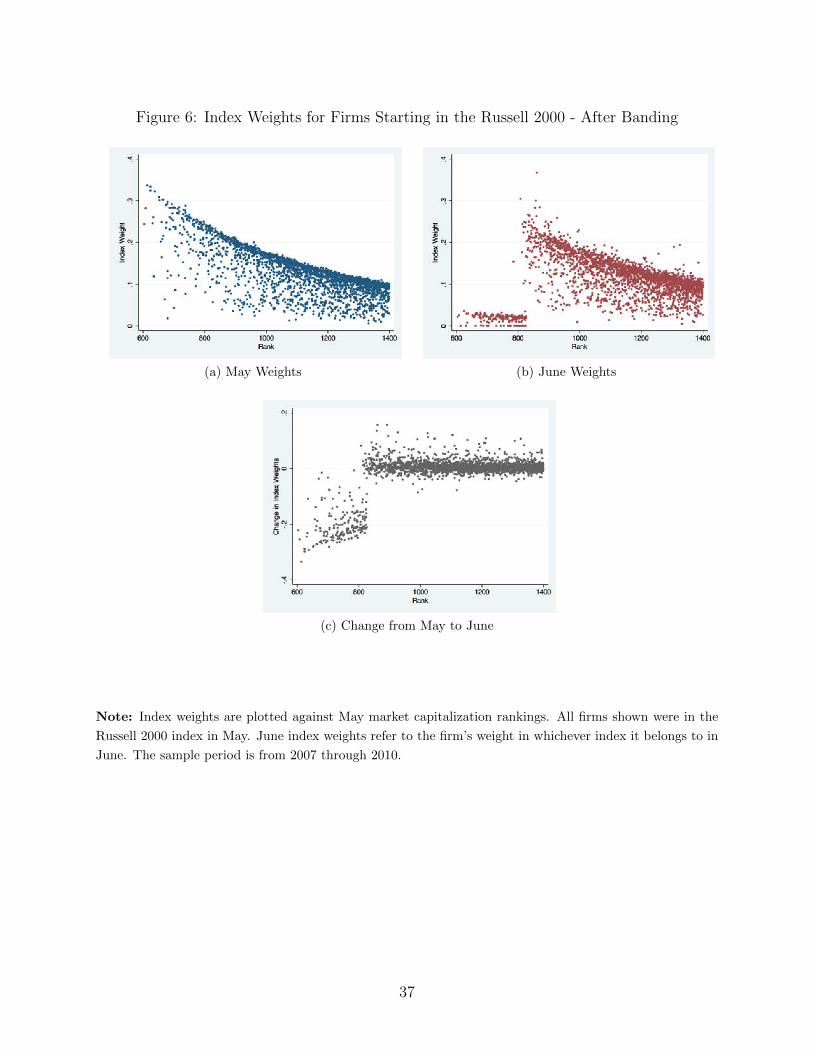
Figure 6: Index Weights for Firms Starting in the Russell 2000 - After Banding
(a) May Weights (b) June Weights
(c) Change from May to June
Note: Index weights are plotted against May market capitalization rankings. All firms shown were in the
Russell 2000 index in May. June index weights refer to the firm’s weight in whichever index it belongs to in
June. The sample period is from 2007 through 2010.
37

Figure 7: Index Weights Around Lower Cutoff for Firms Starting out of the Russell Index
(a) June Weights
Note: Index weights are plotted against May market capitalization rankings. All firms shown were out of
the Russell 2000 index in May. June index weights refer to the firm’s weight in the Russell 2000 index in
June and takes the value 0 if it was not a member of the index. The firms that move into the Russell 2000
are on the left hand side of the cutoff. These are the firms that identify the addition effect. The firms that
stay out of the Russell 2000 are on the right hand side. The sample period is from 2005 through 2012.
38

Figure 8: Index Weights Around Lower Cutoff for Firms Starting in the Russell 2000
(a) May Weights (b) June Weights
(c) Change from May to June
Note: Index weights are plotted against May market capitalization rankings. All firms shown were in the
Russell 2000 index in May. June index weights refer to the firm’s weight in the Russell 2000 index in June
and takes the value 0 if it was not a member of the index. The firms that stay in the Russell 2000 are on the
left hand side of the cutoff. The firms that move out of the Russell 2000 are on the right hand side. These
are the firms that identify the deletion effect. The sample period is from 2005 through 2012.
39

Figure 9: June Returns Around Upper Cutoff - Addition Effect
(a) Bin Width = 2 (b) Bin Width = 5
(c) Bin Width = 10
Note: June returns are plotted against market capitalization ranking. All firms shown were in the Russell
1000 index in May. The firms that stay in the Russell 1000 are on the left hand side of the cutoff. The firms
that move into the Russell 2000 are on the right hand side. These are the firms that identify the addition
effect. The sample period is from 1996 through 2012. The lines drawn fit linear functions of rank on either
side of the cutoff.
40

Figure 10: June Returns Around Upper Cutoff - Deletion Effect
(a) Bin Width = 2 (b) Bin Width = 5
(c) Bin Width = 10
Note: June returns are plotted against market capitalization ranking. All firms shown were in the Russell
2000 index in May. The firms that moved into the Russell 1000 are on the left hand side of the cutoff. These
are the firms that identify the deletion effect. The firms that stayed in the Russell 2000 are on the right
hand side. The sample period is from 1996 through 2012. The lines drawn fit linear functions of rank on
either side of the cutoff.
41

Figure 11: Validity Tests Around Upper Cutoff
(a) May Returns - Addition (b) May Returns - Deletion
(c) Assets - Addition (d) Assets - Deletion
(e) EPS - Addition (f) EPS - Deletion
Note: Outcome variables are plotted against market capitalization ranking. The firms that ended up in the
Russell 1000 are on the left hand side of the cutoff. The firms that ended up in the Russell 2000 are on the
right hand side. The sample period is from 1996 through 2012. The lines drawn fit linear functions of rank
on either side of the cutoff.
42

Table 1: Assets Benchmarked to Indices
Panel A: Passive Assets
1996 1997 1998 1999 2000 2001 2002 2003Russell 2000 11.6 7.6 11.0 13.6 18.9 21.5 26.9 24.6Russell 1000 20.9 20.7 19.0 25.9 17.3 34.0 35.6 37.2
2004 2005 2006 2007 2008 2009 2010 2011Russell 2000 38.9 39.2 43.0 51.7 38.5 38.4 56.8 60.1Russell 1000 84.9 93.3 151.9 175.8 144.8 104.4 137.1 125.8
Panel B: Assets Benchmarked
Number of Products 2002 2003 2004 2005 2006 2007 2008S&P 500 1,009 924 919 901 888 824 685
Russell 2000 289 255 264 275 273 511 449Russell 1000 29 43 43 48 52 52 60
Dollar Amount 2002 2003 2004 2005 2006 2007 2008S&P 500 1,679.8 1,096.9 1,431.8 1,482.9 1,576.7 1,748.6 1,412.1
Russell 2000 198.2 140.7 162.5 201.4 221.1 291.4 263.7Russell 1000 47.6 37.3 66.9 90.0 146.1 172.7 168.6
Note: Panel A reports the dollar amount of passive assets, in billions, benchmarked to Russell 1000 andRussell 2000 by year from Russell’s internal unaudited survey of its clients at the end of June. Panel B reportsthe number of products and dollar amount (in billions) of institutional assets benchmarked to Russell 2000,Russell 1000, and S&P 500. These numbers are taken from Russell Investment’s 2008 US Equity Indexes:Institutional Benchmark Survey. The products surveyed are primarily institutional-oriented mutual funds,separate accounts, and commingled funds at the end of May.
43

Table 2: Summary Statistics
Russell 1000 Russell 2000
Median Mean StDev Median Mean StDevRET 0.007 0.008 0.122 0.007 0.014 0.162
MKTCAP 4.220 12.000 26.300 0.516 0.658 0.496
CORR2000 0.475 0.441 0.261 0.466 0.436 0.259
VOL 0.019 0.023 0.015 0.026 0.031 0.019
ILLIQ 0.053 0.180 1.370 1.020 4.570 20.900
IO 0.722 0.701 0.201 0.642 0.665 6.190
VR 0.967 1.050 0.449 0.949 1.100 0.856
ISSUANCE 0.014 0.232 17.10 0.024 0.116 13.10
SR 0.023 0.037 0.043 0.033 0.053 0.064
REP 1.000 0.683 0.465 0.000 0.477 0.499
ROE 0.133 0.093 4.430 0.093 -1.770 203
ROA 0.046 0.042 0.150 0.035 -0.001 0.217
EPS 1.690 1.780 4.340 0.840 0.717 4.240
ASSET 4,805 21,449 86,939 604 1,079 1,873
C/A 0.038 0.071 0.086 0.051 0.100 0.126
ICR 6.090 73.300 1,127 4.160 72.400 1,537
FLOAT 112,252 289,129 638,581 21,961 29,326 31,097Observations 55842 91198
Note: This table reports monthly summary statistics for all member stocks in the Russell 1000 and Russell2000. RET is monthly stock returns. MKTCAP is in billions of dollars. CORR2000 is the correlation betweendaily stock returns and Russell 2000 index returns, computed monthly. VOL is the standard deviation indaily stock returns, computed monthly. ILLIQ is the Amihud (2002) illiquidity measure, in percentage permillion-dollar volume. IO is institutional ownership. VR is volume ratio. ISSUANCE is the ratio of sharesissued in that fiscal year to initial shares. SR is short ratio. REP is an indicator for repurchase activity inthat fiscal year. EPS is the earnings per share, excluding extraordinary items. ASSET is asset book value inmillions of dollars. C/A is the cash to asset ratio. ICR is the interest coverage ratio. FLOAT is the numberof floating shares (in thousands). The sample period is 1996-2012.
44

Table 3: First Stage of Fuzzy RD
Addition Effect
Upper Cutoff Upper Cutoff After Banding Lower Cutoffτ 0.785∗∗∗ 0.820∗∗∗ 0.862∗∗∗
(31.50) (12.98) (48.86)N 893 164 837adj. R2 0.863 0.845 0.933F 1,876 297 3,896
Deletion Effect
Upper Cutoff Upper Cutoff After Banding Lower Cutoffτ 0.705∗∗∗ 0.759∗∗∗ 0.865∗∗∗
(29.15) (20.90) (39.79)N 1206 340 771adj. R2 0.817 0.878 0.910F 1,799 815 2,601
Note: The table reports the first stage regression from a fuzzy RD design. The outcome variable is anindicator for addition to the Russell 2000 index. The variable τ is an indicator for whether the firm’s rankpredicted addition to the Russell 2000 index. T-statistics are reported in parentheses. All regressions usefirms with end-of-May ranking within 100 spots of the predicted cut-off. The regression specification is linearin ranking by market capitalization on either side of the cut-off. The panel identifying the addition effectonly uses firms that were not in the Russell 2000 at the end of May. The panel identifying the deletion effectonly uses firms that were members of the Russell 2000 at the end of May.* p<0.05, ** p<0.01, *** p<0.001
45

Table 4: Returns Fuzzy RD - Addition Effect
Bandwidth = 50
May Jun Jul Aug Sepp=1 -0.010 0.110∗∗ 0.041 -0.031 0.001
(-0.27) (3.13) (1.04) (-0.76) (0.02)p=2 0.005 0.061 0.180 -0.138 -0.006
(0.04) (0.60) (1.23) (-1.03) (-0.04)N 533 533 531 530 527
Bandwidth = 100
May Jun Jul Aug Sepp=1 -0.003 0.050∗∗ -0.003 0.035 -0.021
(-0.14) (2.65) (-0.11) (1.59) (-0.89)p=2 -0.029 0.110∗∗ 0.085 -0.016 0.014
(-0.68) (2.73) (1.78) (-0.35) (0.29)N 1055 1057 1053 1052 1047
Bandwidth = 200
May Jun Jul Aug Sepp=1 -0.012 0.022 -0.000 0.027 -0.015
(-0.92) (1.84) (-0.02) (1.88) (-1.08)p=2 -0.011 0.060∗∗ 0.001 0.013 -0.023
(-0.47) (2.86) (0.05) (0.55) (-0.89)N 2253 2255 2245 2231 2222
Bandwidth = 300
May Jun Jul Aug Sepp=1 -0.002 0.009 -0.013 0.009 -0.000
(-0.18) (0.91) (-1.07) (0.76) (-0.04)p=2 -0.007 0.036∗ 0.019 0.039∗ -0.023
(-0.38) (2.23) (0.94) (2.08) (-1.20)N 3532 3534 3516 3491 3477
Note: The table reports the results of a fuzzy RD design. The outcome variable is monthly stock returnsand the dependent variable is an indicator for addition to the Russell 2000 index. Monthly returns are shownfor the month immediately preceding the index rebalancing (June) and for four months after. T-statisticsare reported in parentheses. The bandwidth specifies the range of firms that was included on either side ofthe cut-off. For each bandwidth, the RD estimate is shown use both a linear (p=1) and quadratic (p=2)polynomial in firm ranking that is allowed to vary on either sides of the cut-off. Only firms that weremembers of the Russell 1000 index at the end of May are used. The sample period is 1996-2012.* p<0.05, ** p<0.01, *** p<0.001
46

Table 5: Returns Fuzzy RD - Deletion Effect
Bandwidth = 50
May Jun Jul Aug Sepp=1 -0.010 0.052 0.015 -0.006 0.014
(-0.31) (1.64) (0.40) (-0.20) (0.36)p=2 -0.034 -0.050 0.212 0.006 0.064
(-0.35) (-0.49) (1.46) (0.06) (0.48)N 763 762 755 751 746
Bandwidth = 100
May Jun Jul Aug Sepp=1 0.005 0.054∗∗ -0.019 -0.002 0.011
(0.32) (3.00) (-0.96) (-0.09) (0.53)p=2 -0.027 0.052 0.025 -0.000 0.019
(-0.81) (1.48) (0.60) (-0.00) (0.44)N 1546 1545 1533 1526 1519
Bandwidth = 200
May Jun Jul Aug Sepp=1 0.010 0.044∗∗∗ -0.024 -0.004 0.010
(0.94) (3.97) (-1.90) (-0.33) (0.77)p=2 0.007 0.053∗∗ -0.014 0.003 0.005
(0.37) (2.61) (-0.60) (0.14) (0.20)N 3027 3026 3003 2984 2974
Bandwidth = 300
May Jun Jul Aug Sepp=1 0.010 0.029∗∗∗ -0.013 0.004 0.008
(1.13) (3.29) (-1.43) (0.41) (0.84)p=2 0.007 0.053∗∗∗ -0.027 -0.009 0.012
(0.51) (3.61) (-1.64) (-0.59) (0.69)N 4529 4528 4497 4467 4451
Note: The table reports the results of a fuzzy RD design. The outcome variable is monthly stock returnsand the dependent variable is an indicator for staying in the Russell 2000 index. Monthly returns are shownfor the month immediately preceding the index rebalancing (June) and for four months after. T-statisticsare reported in parentheses. The bandwidth specifies the range of firms that was included on either side ofthe cut-off. For each bandwidth, the RD estimate is shown use both a linear (p=1) and quadratic (p=2)polynomial in firm ranking that is allowed to vary on both sides of the cut-off. Only firms that were membersof the Russell 2000 index at the end of May are used. The sample period is 1996-2012.* p<0.05, ** p<0.01, *** p<0.001
47

Table 6: Other Outcome Variables
Addition Effect
May Jun Jul Aug SepCORR 2000 0.034 -0.033 0.047 0.122∗∗ 0.092∗
(0.82) (-0.76) (1.10) (2.79) (2.04)VOL -0.001 0.001 -0.001 0.001 -0.002
(-0.52) (0.23) (-0.26) (0.24) (-0.69)ILLIQ 0.558 0.429 -0.033 0.004 0.136
(0.82) (1.06) (-0.22) (0.02) (0.46)IO 0.031 0.036
(0.77) (0.89)VR -0.010 0.478∗∗ 0.114 0.097 -0.020
(-0.13) (3.14) (1.44) (1.15) (-0.22)ISSUANCE -0.395
(-1.42)SR -0.001 0.002 0.007 0.002 0.005
(-0.14) (0.20) (0.75) (0.22) (0.57)N 920 921 918 915 913
Deletion Effect
May Jun Jul Aug SepCORR 2000 -0.016 0.132∗∗∗ 0.200∗∗∗ 0.058 0.121∗∗
(-0.43) (3.47) (5.06) (1.45) (3.01)VOL 0.001 0.002 0.003 0.003 0.005∗
(0.37) (0.98) (1.11) (1.36) (2.02)ILLIQ 0.085 0.005 -0.105 -0.743 -0.216
(0.11) (0.01) (-0.29) (-0.83) (-0.39)IO -0.063 -0.037
(-1.69) (-1.02)VR 0.151 -0.263∗∗ 0.050 0.106 0.166
(0.79) (-2.74) (0.55) (1.55) (1.64)ISSUANCE 0.115
(0.44)SR 0.001 -0.000 0.010 0.012 0.011
(0.14) (-0.02) (1.16) (1.43) (1.31)N 1308 1309 1300 1295 1284
Note: The table reports the results of a fuzzy RD design. The dependent variable is an indicator foraddition the Russell 2000 index. All regressions use firms with end-of-May ranking within 100 spots of thepredicted cut-off. The regression specification is linear in ranking and is allowed to vary on either side of thecut-off. Only firms that were members of the Russell 1000 index at the end of May are used to estimate theaddition effect. Only those that were members of the Russell 2000 are used for the deletion effect. Issuanceis defined for the fiscal year. Definitions of fiscal year vary by company but always include the June followingreconstitution. The sample period is 1996-2012.* p<0.05, ** p<0.01, *** p<0.001
48

Table 7: Validity Tests
Addition Effect
MKTCAP REP ROE ROA EPS ASSETS ICR C/A FLOAT0.003 -0.055 -1.243 0.069 -0.042 -789.443 18.737 0.021 -786.479(0.06) (-0.59) (-0.37) (1.36) (-0.11) (-1.39) (0.22) (1.09) (-0.07)
N 1057 747 887 887 886 888 782 866 1057
Deletion Effect
MKTCAP REP ROE ROA EPS ASSETS ICR C/A FLOAT0.031 -0.053 -0.927 -0.025 0.898 -89.741 -159.523 0.009 -2203.850(0.41) (-0.64) (-0.98) (-0.84) (0.70) (-0.26) (-1.14) (0.45) (-0.35)
N 1546 1005 1237 1237 1237 1237 1081 1219 1546
Note: The table reports the results of a fuzzy RD design. The outcome variables are fundamental firmvariables and the dependent variable is an indicator for addition to the Russell 2000 index. The data onfundamental variables is annual so estimates cannot be reported separately for each month. T-statistics arereported in parentheses. All regressions use firms with end-of-May ranking within 100 spots of the predictedcut-off. The regression specification is linear in ranking and is allowed to vary on either side of the cut-off.Only firms that were members of the Russell 1000 index at the end of May are used to estimate the additioneffect. Only those that were members of the Russell 2000 are used for the deletion effect. The sample periodis 1996-2012.* p<0.05, ** p<0.01, *** p<0.001
49

Table 8: Lower Cut-off Returns
Addition Effect
May Jun Jul Aug Sep-0.034 0.036 0.022 -0.031 0.029(-1.09) (1.45) (1.02) (-1.29) (1.25)
N 822 835 829 823 813
Deletion Effect
May Jun Jul Aug Sep0.015 0.033 0.058∗ -0.054 0.055∗
(0.52) (1.25) (1.97) (-1.82) (2.00)N 770 771 766 765 764
Note: The table reports the results of a fuzzy RD design. The outcome variable is monthly stock returns andthe dependent variable is an indicator for addition to the Russell 2000 index. Monthly returns are shown forthe month immediately preceding the index rebalancing (June) and for four months after. The instrumentfor addition is an indicator for firms with ranking 3000 or less. T-statistics are reported in parentheses.Allregressions use firms with end-of-May ranking within 100 spots of the predicted cut-off. For both additionand deletion, the RD estimate is shown use both a linear (p=1) and quadratic (p=2) polynomial in firmranking that is allowed to vary on either sides of the cut-off. Only firms that were not members of the Russell3000 index at the end of May are used to estimate addition. Only those that were members of the Russell2000 index at the end of May are used to estimate deletion. The sample period is 2005-2012.* p<0.05, ** p<0.01, *** p<0.001
50

Table 9: Lower Cut-off Outcome Variables
Addition Effect
May Jun Jul Aug SepCORR 2000 0.009 0.029 0.250∗∗∗ 0.283∗∗∗ 0.242∗∗∗
(0.17) (0.63) (5.06) (5.92) (4.35)VOL -0.001 0.005 0.002 0.005 0.003
(-0.26) (1.55) (0.57) (1.34) (0.77)ILLIQ 3.516 -3.679 -23.593∗ -1.236 -8.204
(0.24) (-0.60) (-2.16) (-0.13) (-1.08)IO 0.012 0.009
(0.30) (0.22)VR -0.750 3.332∗∗∗ 0.332∗∗ 0.091 -0.231
(-1.86) (7.02) (2.91) (0.62) (-1.01)ISSUANCE 0.094
(0.43)SR -0.008 -0.002 0.021∗∗ 0.021∗∗ 0.019∗∗
(-1.16) (-0.34) (2.80) (2.80) (2.68)N 496 502 499 495 489
Deletion Effect
May Jun Jul Aug SepCORR 2000 -0.006 0.061 0.181∗∗∗ 0.352∗∗∗ 0.281∗∗∗
(-0.12) (1.39) (3.60) (6.97) (5.21)VOL 0.001 -0.000 0.005 0.003 0.006
(0.24) (-0.08) (1.20) (0.76) (1.48)ILLIQ -5.105 -0.819 -0.231 -1.927 -4.393
(-0.94) (-0.41) (-0.13) (-0.89) (-1.10)IO 0.031 0.041
(0.78) (1.04)VR -0.093 -1.530∗∗∗ 0.196 0.046 0.406∗∗∗
(-0.78) (-6.00) (1.96) (0.36) (3.72)ISSUANCE -0.456
(-1.45)SR -0.005 -0.002 0.020∗∗ 0.021∗∗ 0.018∗∗
(-0.62) (-0.21) (2.59) (2.93) (2.63)N 581 580 577 575 574
Note: The table reports the results of a fuzzy RD design. The dependent variable is an indicator for additionto the Russell 2000 index. T-statistics are reported in parentheses. All regressions use firms with end-of-Mayranking within 100 spots of the predicted cut-off. The regression specification is linear in ranking and isallowed to vary on either side of the 3000 cut-off. The instrument for addition is an indicator for firms withranking 3000 or less. Only firms that were not members of the Russell 3000 index at the end of May are usedto estimate the addition effect. Only those that were members of the Russell 2000 are used for the deletioneffect. Issuance is defined for the fiscal year. Definitions of fiscal year vary by company but always includethe June following reconstitution.The sample period is 2005-2012.* p<0.05, ** p<0.01, *** p<0.001
51

Table 10: Lower Cut-off Validity Tests
Addition Effect
MKTCAP REP ROE ROA EPS ASSETS ICR C/A0.013 0.090 0.196 0.001 0.033 -43.161 -159.180 0.061(1.44) (0.78) (0.84) (0.02) (0.11) (-0.37) (-1.57) (1.57)
N 837 357 396 396 395 396 315 393
Deletion Effect
MKTCAP REP ROE ROA EPS ASSETS ICR C/A-0.011 0.094 0.126 -0.012 -0.400 -49.995 24.090 0.030(-1.06) (0.90) (0.83) (-0.27) (-1.14) (-0.34) (0.03) (0.87)
N 771 458 501 501 500 502 394 494
Note: The table reports the results of a fuzzy RD design. The outcome variables are fundamental firmvariables and the dependent variable is an indicator for addition to the Russell 2000 index. The data onfundamental variables is annual so estimates cannot be reported separately for each month. T-statistics arereported in parentheses. All regressions use firms with end-of-May ranking within 100 spots of the predictedcut-off. The regression specification is linear in ranking and is allowed to vary on either side of the 3000cut-off. The instrument for addition is an indicator for firms with ranking 3000 or less. Only firms that werenot members of the Russell 3000 index at the end of May are used to estimate the addition effect. Only thosethat were members of the Russell 2000 are used for the deletion effect. The sample period is 2005-2012.* p<0.05, ** p<0.01, *** p<0.001
52