Research ArticleFault Modeling and Testing for Analog Circuits in ComplexSpace Based on Supply Current and Output Voltage

Hongzhi Hu12 Shulin Tian1 and Qing Guo2

1School of Automation Engineering University of Electronic Science and Technology of China Chengdu 611731 China2Guangxi Key Laboratory of Automatic Detecting Technology and Instrument Guilin University of Electronic TechnologyGuilin 541004 China

Correspondence should be addressed to Hongzhi Hu huhzgueteducn

Received 14 October 2014 Revised 22 February 2015 Accepted 23 February 2015

Academic Editor Hossein Torkaman

Copyright copy 2015 Hongzhi Hu et al This is an open access article distributed under the Creative Commons Attribution Licensewhich permits unrestricted use distribution and reproduction in any medium provided the original work is properly cited

This paper deals with the modeling of fault for analog circuits A two-dimensional (2D) fault model is first proposed based oncollaborative analysis of supply current and output voltage This model is a family of circle loci on the complex plane and itsimplifies greatly the algorithms for test point selection and potential fault simulations which are primary difficulties in faultdiagnosis of analog circuits Furthermore in order to reduce the difficulty of fault location an improved fault model in three-dimensional (3D) complex space is proposed which achieves a far better fault detection ratio (FDR) against measurement errorand parametric tolerance To address the problem of fault masking in both 2D and 3D fault models this paper proposes an effectivedesign for testability (DFT) method By adding redundant bypassing-components in the circuit under test (CUT) this methodachieves excellent fault isolation ratio (FIR) in ambiguity group isolation The efficacy of the proposed model and testing methodis validated through experimental results provided in this paper

1 Introduction

Over the past two decades fault detection and diagnosis ofanalog circuits become an important research area wherea number of corresponding theories and techniques havebeen developed Among the researches in this area faultdictionary is one of the most important methods that haveattracted great interests [1ndash5] Various circuit variables (egvoltage current and frequency) have been used in faultdictionary to obtain fault signatures [6ndash8] In addition to thecommonly employed measurement of output voltage supplycurrent testing has been applied widely in analog and mixedsignal integrated circuits (ICs) with excellent fault coverageespecially for the catastrophic fault of CMOS ICs [9ndash11]

Despite the advantages of fault dictionary there arestill persistent challenges such as test point selection andpotential faults simulations in applications of fault dictionarymethod for fault diagnosis of analog circuits Wang and Yangproposed a slope fault mode which not only reduces therequired number of test points to two but also simplifiesthe potential fault simulation greatly [2] However the slope

fault model is only limited to dynamic circuits To achievedetection of parametric faults for analog circuits Yang et alproposes a complex-circle based fault model [3] Althoughthis proposed faultmodel is improved sequentially by optimaltesting frequency selection [12] and fault location [13] theweakness of fault masking still remains Moreover a 3Dmodel based on transfer function was proposed in [14]it extends the distances between fault loci and improvesthe practicability for applications Recently Ma and Wangachieved detecting catastrophic faults and parametric faultsby analyzing the harmonic spectrum of output voltage andsupply current [11] Following the ideas of these researchesthis paper proposes two improved fault models with satisfac-tory FDR based on collaborative analysis of output voltageand supply current Moreover to isolate ambiguity groups adesign for testability (DFT) method is proposed to achievebetter fault isolation ratio (FIR) against the influence ofanalog tolerance and measurement errors

This paper is organized as follows First the theory ofcollaborative fault model on 2D complex plane is introducedin Section 2 An example of a Sallen-Key filter is also provided

Hindawi Publishing CorporationJournal of Applied MathematicsVolume 2015 Article ID 851837 9 pageshttpdxdoiorg1011552015851837

2 Journal of Applied Mathematics

to illustrate the theory in this section In order to reducethe difficulty of fault location and isolation an improvedfault model in 3D complex space is proposed in Section 3Furthermore to deal with the ambiguity groups in the faultmodel an innovative method of DFT is demonstrated inSection 4 to improve the FIR Validation of the proposedmethod is provided by PSPICE Finally conclusions andfuture work are summarized in Section 5

2 Collaborative Fault Model on2D Complex Plane

21 Theorem of the 2D Collaborative Fault Model A lineartime-invariant passive CUT 119873 is assumed to contain 119899

components 119865119894(1 le 119894 le 119899) 119873 is assumed to be stimulated

by a direct current (DC) power source 119880119889119889

and a family ofalternating current (AC) signals 119880

119904119896(1 le 119896 le 119898) where 119898 is

the number of AC signals Then a (119898 + 1)-dimension vectorUS is composed as follows

US = (119880119889119889 1198801199041

1198801199042

sdot sdot sdot 119880119904119898) (1)

Furthermore a single component 119875 is assumed to be thepotential failure component in 119873 where

119875 isin 119865119894| 1 le 119894 le 119899 (2)

The voltage across 119875 is defined as 119906119865 According to the

Substitution Theorem a voltage source 119906119865can be used to

replace the component 119875 in the CUTTherefore both voltage119906119865and vector US are regarded as the excitation of the CUT

Then the collaborative output 119865119888(sdot) is defined as follows

119865119888 (119904 119875) = (119880119900 119868

119889119889) (

1198880

1198881

) (3)

where 119880119900is the output voltage of CUT 119868

119889119889is the power

supply current and 119904 is the Laplacian operator 1198880and 1198881

are predefined coefficients Furthermore the correspondingtransfer function matricesH andHF are defined as

H = (

1198671119889119889 (119904) 119867

11 (119904) sdot sdot sdot 1198671119898 (119904)

1198672119889119889 (119904) 119867

21 (119904) sdot sdot sdot 1198672119898 (119904)

)

119879

HF = (1198671119865 (119904) 1198672119865 (119904))

(4)

where 1198671119889119889

(119904) 1198672119889119889

(119904) 1198671119896

(119904) (1 le 119896 le 119898) 1198672119896

(119904) (1 le 119896 le

119898) 1198671119865

(119904) and 1198672119865

(119904) are transfer functions with respect to119880119900and 119868119889119889 Then 119865

119888(sdot) can be expressed as

119865119888 (119904 119875) = (USH + 119906

119865HF) (

1198880

1198881

) (5)

In addition according to the theories of circuit analysis119906119865can be further defined as

119906119865

= 119906oc119885119865

1198850+ 119885119865

(6)

where 119906oc is open circuit voltage for the failure component 1198751198850is corresponding Thevenin equivalent impedance while

119885119865is the impedance of 119875 According to the Theveninrsquos

Theorem 119906oc and 1198850are independent of 119885

119865 Therefore

119865119888 (119904 119875) = USH(

1198880

1198881

) + 119906ocHF (

1198880

1198881

)119885119865

1198850+ 119885119865

(7)

For any determinate frequency 120596 the Laplacian operator119904 = 119895120596 is also an imaginary constant where 119895 is imaginaryunit vector In addition without loss of generality 119885

119865can

be assumed to be a pure resistance 119877119865or reactance 119883

119865

Therefore taking 119877119865as an example

119865119888 (119875) = USH(

1198880

1198881

) + 119906ocHF (

1198880

1198881

)119877119865

1198850+ 119877119865

(8)

With the following assumptions

USH(

1198880

1198881

) = 1198861+ 1198951198871

119906ocHF (

1198880

1198881

) = 1198862+ 1198951198872

1198850= 1198770+ 1198951198830

(9)

where 1198861 1198871 1198862 1198872 1198770 and 119883

0are all real numbers then

119865119888 (119875) = (119886

1+ 1198951198871) + (119886

2+ 1198951198872)

119877119865

(1198770+ 1198951198830) + 119877119865

1198770+ 1198951198830

119877119865

=[1198862(119865119877minus 1198861) + 1198872(119865119868minus 1198871)]

(119865119877minus 1198861)2+ (119865119868minus 1198871)2

minus 1

+ 119895[minus1198862(119865119868minus 1198871) + 1198872(119865119877minus 1198861)]

(119865119877minus 1198861)2+ (119865119868minus 1198871)2

(10)

where

119865119877

= Re [119865119888 (119875)]

119865119868= Im [119865

119888 (119875)]

(11)

If 1198770and 119883

0are all equal to zero the CUT is equal to an

ideal voltage source 119906oc corresponding to the component 119875This means that variation in 119885

119865will not affect 119906

119865and 119865

119888(119875)

Thus we have

1198770

119877119865

=[1198862(119865119877minus 1198861) + 1198872(119865119868minus 1198871)]

(119865119877minus 1198861)2+ (119865119868minus 1198871)2

minus 1

1198830

119877119865

=[minus1198862(119865119868minus 1198871) + 1198872(119865119877minus 1198861)]

(119865119877minus 1198861)2+ (119865119868minus 1198871)2

(12)

Then

1198770

1198830

=1198862(119865119877minus 1198861) + 1198872(119865119868minus 1198871) minus (119865

119877minus 1198861)2minus (119865119868minus 1198871)2

minus1198862(119865119868minus 1198871) + 1198872(119865119877minus 1198861)

(13)

Journal of Applied Mathematics 3

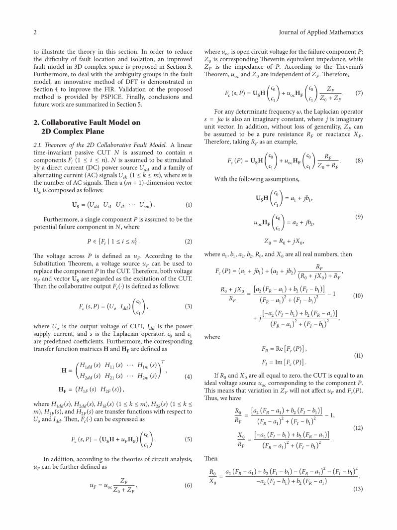
Furthermore (13) can be transformed into a formula of 2Dcircle

(119865119877minus 119888119903)2+ (119865119868minus 119888119895)2

= 119903119888

2 (14)

119888119903=

minus11988721198770+ 211988611198830+ 11988621198830

21198830

119888119895=

11988621198770+ 211988711198830+ 11988721198830

21198830

119903119888

2=

(1198862

2+ 1198872

2) (1198770

2+ 1198830

2)

41198830

2

(15)

where 119888119903and 119888119895are the real part and imaginary part of the

circle center coordinates respectively 119903119888is the radius It is

confirmed that 119888119903 119888119895 and 119903

119888are independent of the parametric

change of the failure component119875Therefore fault loci fittingrequires a small amount of simulation on potential faults forboth catastrophic faults and parametric faults Alternativelyif119885119865is assumed to be a pure reactance119883

119865 similar conclusion

can be reachedFor a CUT with 119899 components 119875

119894(1 le 119894 le 119899) fault

modeling is to determine the model parameters 119888119903119894 119888119895119894 and

119903119888119894for each 119875

119894according to (15) where parameters 119888

119903119894 119888119895119894

and 119903119888119894are corresponding to 119888

119903 119888119895 and 119903

119888 respectively In

most actual analog cases (14) is hard to derive from transferfunction directly However it is well known that three setsof distinct data are sufficient to determine a circle In thisregard simulation is a simple method to establish the circlemodel in (14) Therefore in the modeling process three setsof distinct output data are obtained by parametric sweepsimulations corresponding to three distinct values of eachcomponent 119875

119894 For the whole CUT 119899 parametric sweep

simulations are needed Three sets of distinct simulationdata for each component are assumed as 119865

0

119888 1198651

119888119894 and 119865

2

119888119894

Since 1198650

119888is assumed to be the fault free output it fits in

with all componentsThe fault modeling process is illustratedin Figure 1 In addition the following equation is used tocalculate the parameters 119888

119903119894 119888119895119894 and 119903

119888119894for component 119875

119894(1 le

119894 le 119899)

[Re (1198650

119888) minus 119888119903119894]2

+ [Im (1198650

119888) minus 119888119895119894]2

= 119903119888119894

2

[Re (1198651

119888119894) minus 119888119903119894]2

+ [Im (1198651

119888119894) minus 119888119895119894]2

= 119903119888119894

2

[Re (1198652

119888119894) minus 119888119903119894]2

+ [Im (1198652

119888119894) minus 119888119895119894]2

= 119903119888119894

2

(16)

22 Example of a Sallen-Key Filter Compared with the diffi-culty of obtaining explicit mathematical expression simula-tion is a relatively easyway for faultmodeling Todemonstratethe method a second-order Sallen-Key filter as shown inFigure 2 is adopted as an example of circuit under test (CUT)By parameter sweeping simulationswith respect to the supplycurrent 119868

119889119889and the output response 119880

119900in PSPICE the 2D

collaborative fault model can be achieved The simulationresults are listed in Table 1 in which parametric ratio meansthe ratio between failure value and nominal value for each

Start

End

Yes

No

Simulating two distinct output data F1ci and F

2ci for component

Pi by parametric sweep simulation

Calculating parameters cri cji and rci for component

Simulating and recording the fault free output F0c

Parametric sweep simulation time i = 1

Pi according to (16)

i = i + 1 if i gt n

Figure 1 Flowchart of fault modeling

R1

R2

R3 R4

C1

C2

OutU1

Vss

+

minus

119828119826

Uo

Idd

Vdd

Figure 2 Second-order Sallen-key filter where 1198771 1198772 1198773 and 1198774

are 10 kΩ 1198621 and 1198622 are 47 nF

component Further results are also provided in Figure 3Thestimulation is a 3 kHz 1 V sine signal and the parametersweeping range for each component is assumed to be from119901119894times10minus4 to119901

119894times104 where119901

119894(1 le 119894 le 119899) is the fault-free value

of the 119894th component 119865119894 In addition the simulation range

of 1198773 and 1198774 is reduced because output power of the filteris limited As shown in Figure 3 all potential fault statusescompose a family of loci on the complex plane which iscalled 119865

119894-loci Every 119865

119894-locus corresponds to all the potential

fault statuses of a component not only parametric faults butalso catastrophic faults Furthermore119865

119894-loci converges in the

fault free point A and zero point BNote that in some cases distances between some 119865

119894-loci

are very small In extreme cases some 119865119894-loci may coincide

with each other which results in ambiguity group Since the2D collaborative faultmodel is derived from transfer functionof CUT ambiguity group may be an inevitable problem [15]Table 2 lists the ambiguity groups of the Sallen-Key filter and

4 Journal of Applied Mathematics

Table 1 Simulation results of 2D model for the Sallen-Key filter

Parametricratio

Collaborative simulation results119865119862(1198771) 119865

119862(1198772) 119865

119862(1198773) 119865

119862(1198774) 119865

119862(1198621) 119865

119862(1198622)

001 07977 minus 11989510218 17383 minus 11989503307 mdash minus00364 minus 11989504066 11249 + 11989506892 02792 minus 11989508047

005 07959 minus 11989510537 17801 minus 11989504091 mdash minus00369 minus 11989504382 12076 + 11989506979 02816 minus 11989508265

008 07925 minus 11989510777 18094 minus 11989504733 mdash minus00373 minus 11989504627 12755 + 11989507012 02830 minus 11989508264

01 07906 minus 11989510949 18271 minus 11989505187 mdash minus00375 minus 11989504794 13282 + 11989507019 02839 minus 11989508519

04 07063 minus 11989513735 17917 minus 11989514096 mdash minus00348 minus 11989507801 24864 + 11989502002 02905 minus 11989510578

07 04829 minus 11989516766 09513 minus 11989520720 07186 minus 11989539260 minus00105 minus 11989512155 19996 minus 11989523457 02565 minus 11989513783

09 02312 minus 11989518427 03137 minus 11989520195 01476 minus 11989522588 00354 minus 11989516315 04333 minus 11989522252 01647 minus 11989517011

10 00767 minus 11989518977 00767 minus 11989518977 00767 minus 11989518977 00767 minus 11989518977 00767 minus 11989518977 00767 minus 1198958977

11 minus09320 minus 11989519275 minus01008 minus 11989517530 00385 minus 11989516543 01390 minus 11989522194 minus01113 minus 11989516025 minus00746 minus 11989521441

13 minus04407 minus 11989518928 minus03146 minus 11989514630 00013 minus 11989513453 03832 minus 11989530993 minus02476 minus 11989511936 minus06829 minus 11989526877

15 minus07474 minus 11989517426 minus04093 minus 11989512169 minus00151 minus 11989511573 10301 minus 11989545183 minus02751 minus 11989509275 minus20075 minus 11989529003

2 minus11278 minus 11989511435 minus04420 minus 11989508107 minus00304 minus 11989509029 15264 minus 11989531208 minus02445 minus 11989505844 minus28027 + 11989505055

3 minus09616 minus 11989503874 minus03514 minus 11989504570 minus00366 minus 11989507040 mdash minus01726 minus 11989503330 minus07652 + 11989506990

5 minus05445 minus 11989500583 minus02246 minus 11989502339 minus00379 minus 11989505686 mdash minus01030 minus 11989501748 minus02644 + 11989503346

10 minus02431 + 11989500129 minus01143 minus 11989501029 minus00375 minus 11989504793 mdash minus00509 minus 11989500800 minus00979 + 11989501423

30 minus00739 + 11989500104 minus00383 minus 11989500314 minus00367 minus 11989504248 mdash minus00168 minus 11989500252 minus00273 + 11989500425

100 minus00215 + 11989500036 minus00115 minus 11989500091 minus00364 minus 11989504067 mdash minus00050 minus 11989500074 minus00078 + 11989500124

0 5 10

0

5

5

1

2

3

4

minus5

minus5minus10

Im(F

C)

Re(FC)

A

B

Figure 3 2D collaborative fault model of the Sallen-Key filter Allpotential fault statuses of the filter compose a family of 119865

119894-loci and

119865119894-loci converge in the fault free point A and zero point B

Figure 3 shows that while the 119865119894-loci of 1198771 1198772 1198621 and 1198622

are obviously different from others fault status of 1198773 and 1198774

are located on the same locusThismeans that potential faultsof 1198773 and 1198774 cannot be isolated based on the fault model inFigure 3 therefore 1198773 and 1198774 fall into the same ambiguitygroup 1198773 1198774

3 Fault Modeling in 3D Complex Space

Based on the measurements of supply current and voltageresponse at any test point the 2D collaborative fault model

Table 2 Ambiguity groups of the Sallen-Key filter

Ambiguity group Fault componentsA 1198771

B 1198772

C 1198773 1198774

D 1198621

E 1198622

transforms all potential failure statuses into a family of lociTherefore both parametric faults and catastrophic faults canall be detected and located However due to the limits ofcomponent tolerance and measurement error the 2D faultmodel is difficult to apply in actual analog circuits Asdepicted in Figure 3 between point A and point B the 1198772

and 1198621-loci are too close to be distinguished Therefore toincrease the practicability for actual applications the 2D faultmodel is extended into 3D complex space

31 Theorem of 3D Collaborative Fault Model The 2D func-tion in (3) is a linear combination of supply current 119868

119889119889and

voltage response 119880119900 based on the measurements of real part

Re(sdot) and imaginary part Im(sdot) of each complex variable119868119889119889

and 119880119900are easier to measure in-circuit from limited

test points than other circuit variables such as the inputadmittance Furthermore the complex modulus (absolutevalue) | sdot | is also employed to compose the 3D function Thishelps to increase the distance between 119865

119894-loci fault models

and improve the FIRSimilarly the component 119875 in (2) is still assumed to be

the failure component Therefore by defining 119909 119910 and 119911 as

Journal of Applied Mathematics 5

Table 3 Simulation results for 1198772 and 1198621 in 3D model

Parametric ratio Simulation results of 1198772 Simulation results of 1198621

119865119880(1198772) 119865

119868119863119863(1198772) 119888

1119868119889119889

119865119880(1198621) 119865

119868119863119863(1198621) 119888

1119868119889119889

001 2052 minus 1198950040 23371 minus03137 minus 11989502910 1156 + 1198951009 31270 minus00276 minus 11989503186

005 2115 minus 1198950121 22642 minus03349 minus 11989502879 1251 + 1198951034 29564 minus00380 minus 11989503361

008 2161 minus 1198950189 2116 minus03516 minus 11989502843 1328 + 1198951051 28331 minus00472 minus 11989503498

01 2190 minus 1198950238 21782 minus03629 minus 11989502812 1382 + 1198951061 27540 minus00538 minus 11989503591

04 2323 minus 1198951263 18144 minus05313 minus 11989501466 2804 + 1198950713 16581 minus03176 minus 11989505127

07 1491 minus 1198952184 18142 minus05397 + 11989501120 2743 minus 1198952293 13418 minus07434 minus 11989500527

09 0752 minus 1198952248 20242 minus04380 + 11989502285 0929 minus 1198952460 18244 minus04953 + 11989502348

10 0457 minus 1198952155 21775 minus03804 + 11989502573 0457 minus 1198952155 21775 minus03804 + 11989502573

11 0226 minus 1198952024 23555 minus03268 + 02710 0185 minus 1198951854 25751 minus02959 + 11989502515

13 minus0075 minus 1198951734 27645 minus02396 + 11989502710 minus0051 minus 1198951413 33929 minus01970 + 11989502194

15 minus0231 minus 1198951471 32227 minus01781 + 11989502541 minus0134 minus 1198951114 42771 minus01410 + 11989501865

2 minus0348 minus 1198951013 44787 minus00945 + 11989502023 minus0166 minus 1198950716 65293 minus00787 + 11989501314

3 minus0313 minus 1198950591 71763 minus00386 + 11989501339 minus0133 minus 1198950414 110258 minus00401 + 11989500814

5 minus0211 minus 1198950311 127565 minus00133 + 11989500773 minus0084 minus 1198950220 203875 minus00193 + 11989500451

10 minus0111 minus 1198950140 268834 minus00036 + 11989500370 minus0043 minus 1198950101 436119 minus00083 + 11989500214

30 minus0038 minus 1198950043 835634 minus00006 + 11989500120 minus0014 minus 1198950032 1365537 minus00025 + 11989500069

100 minus0011 minus 1198950013 2818780 minus00001 + 11989500035 minus0004 minus 1198950009 4618366 minus00007 + 11989500020

the unit vectors in 3D complex space a transformationfunction 119865

1

3D(sdot) can be composed as follow [14]

1198651

3D (119875) = 119909 sdot Re [119865119880 (119875)]

+ 119910 sdot Im [119865119880 (119875)] + 119911 sdot

10038161003816100381610038161003816100381610038161003816

1

119865119868119863119863 (119875)

10038161003816100381610038161003816100381610038161003816

(17)

where

119865119880 (119875) = 119888

0119880119900 (18)

119865119868119863119863 (119875) =

1

(1198881119868119889119889

) (19)

where 1198880and 1198881are still adjustment coefficients as in (3)

Taking the component pair1198772-1198621 as an example the distance1198631

3D(sdot) between 1198772 and 1198621-loci is

1198631

3D (1198772 1198621)

= radic[1198631119909(1198772 1198621)]

2+ [1198631119910(1198772 1198621)]

2

+ [1198631119911(1198772 1198621)]

2

(20)

where 1198631

119909(sdot) 1198631119910(sdot) and 119863

1

119911(sdot) are distances corresponding to

each axe in 3D complex space

1198631

119909(1198772 1198621) =

1003816100381610038161003816Re [119865119880 (1198772)] minus Re [119865

119880 (1198621)]1003816100381610038161003816

1198631

119910(1198772 1198621) =

1003816100381610038161003816Im [119865119880 (1198772)] minus Im [119865

119880 (1198621)]1003816100381610038161003816

1198631

119911(1198772 1198621) =

10038161003816100381610038161003816100381610038161003816

10038161003816100381610038161003816100381610038161003816

1

119865119868119863119863 (1198772)

10038161003816100381610038161003816100381610038161003816

minus

10038161003816100381610038161003816100381610038161003816

1

119865119868119863119863 (1198621)

10038161003816100381610038161003816100381610038161003816

10038161003816100381610038161003816100381610038161003816

(21)

Although the distance 1198631

3D(sdot) in (20) has been proved tobe better than that in 2D 119865

119894-loci fault model [14] it is calcu-

lated based on voltage and input admittance whose absolute

values are usually far greater than supply current Thereforefor an appropriate coefficient 119888

1 the following inequality can

be guaranteed10038161003816100381610038161003816100381610038161003816

1

119865119868119863119863 (119875)

10038161003816100381610038161003816100381610038161003816

=10038161003816100381610038161198881119868119889119889

1003816100381610038161003816 lt 1 (22)

In addition a new distance 1198632

119911(sdot) is defined as follows

1198632

119911(1198772 1198621) =

1003816100381610038161003816

1003816100381610038161003816119865119868119863119863 (1198772)1003816100381610038161003816 minus

1003816100381610038161003816119865119868119863119863 (1198621)1003816100381610038161003816

1003816100381610038161003816

1198632

119911(1198772 1198621) =

1198631

119911(1198772 1198621)

11003816100381610038161003816119865119868119863119863 (1198772)

1003816100381610038161003816 sdot 11003816100381610038161003816119865119868119863119863 (1198621)

1003816100381610038161003816

gt 1198631

119911(1198772 1198621)

(23)

Therefore a new transformation function 1198652

3D(sdot) for the3D fault model can be defined as

1198652

3D (119875) = 119909 sdot Re [119865119880 (119875)] + 119910 sdot Im [119865

119880 (119875)] + 119911 sdot1003816100381610038161003816119865119868119863119863 (119875)

1003816100381610038161003816

(24)

Furthermore the distance 1198632

3D(sdot) is defined for the newfunction 119865

2

3D(sdot) Taking 1198772 and 1198621 as an example it can beexpressed as

1198632

3D (1198772 1198621)

= radic[1198631119909(1198772 1198621)]

2+ [1198631119910(1198772 1198621)]

2

+ [1198632119911(1198772 1198621)]

2

(25)

32 Simulation Example of Sallen-Key Filter for the 3DModelFor a given input of 1 V 3 kHz sine signal PSPICE results onthe Sallen-Key filter are obtained The key part of simulationresults are listed in Table 3 The original simulation results

6 Journal of Applied Mathematics

0

0

10

20

30

40

50

60

0

minus4

minus4minus2

minus2

5

1

2

3

4

A

B

Re[FU(P)] (V)

Im[F

U(P)]

(V)

|FID

D(P)|

(A)

Figure 4 Family of fault loci in 3D complex place for the Sallen-Keyfilter All119865

119894-loci converge in the fault free point A while some119865

119894-loci

have tendency to an infinity point B

include 119880119900and 119868

119889119889 corresponding to all potential failure

status of each component such as 1198772 and 1198621 and then allthe data in Table 3 is obtained according to (18) and (19)Moreover the simulation results are also illustrated integrallyin Figure 4 It shows that all 119865

119894-loci converge in the fault free

point A which is similar to the 2D 119865119894-loci However due

to the definition in (19) some 119865119894-loci tend to be an infinity

point B instead of the determinate point B in 2D model Theassociated ambiguity groups are the same as shown inTable 2

To validate the improvement of fault model 11986523D(sdot) in (24)

the 2D model proposed in Section 2 is used as a referenceIn addition both the 3D model 119865

1

3D(sdot) proposed in [14]and the complex-circle-based fault model proposed in [1213] are adopted for comparison In the example of 1198772 and1198621 in the Sallen-Key filter distances between 1198772 and 1198621-loci are provided in Table 4 according to each fault modelrespectively the comparison range is from119901

119894times10minus2 to119901

119894times102

where 119901119894is the fault-free value of 1198772 and 1198621 The results of

comparison between different methods are also illustrated inFigure 5 in which the curve 1198891 is the distance of 1198772-1198621 inthe 3D model 1198652

3D(sdot) the curve 1198892 is the distance defined inthe 2Dmodel the dash curve 1198893 is defined by 119865

1

3D(sdot) [14] anddash curve 1198894 is related to complex-circle-based fault model[12 13] As shown in Table 4 1198893 is better than 1198894 howeverbecause the biggest gap between 1198893 and 1198894 is less than 221198894 is very close to 1198893 in Figure 5 Moreover 1198891 is much betterthan all the others Since 1198893 is also based on the 3D modelin [14] it is taken as an ideal reference On average 1198891 is96 bigger than 1198893 in the value range from 119901

119894times 10minus2 to 119901

119894

Moreover in the range from 119901119894to 119901119894times102 because 119868

119889119889and119880

119900

tend to be zero 1198891 increases continuously while 1198893 reduces

Table 4 Distances between 1198772 and 1198621-loci with respect to differentfault models

Parametric ratio 1198891 1198892 1198893 1198894

001 15896 11902 13836 13805005 16000 12463 14463 14453008 16180 12902 14971 1496301 16342 13184 15324 1529404 20396 17533 20343 2033607 13426 10835 12716 1256709 03408 02379 02814 0276110 0 0 0 011 02808 01509 01787 0175013 07061 02776 03288 0321915 11175 03190 03778 037002 20800 03004 03553 034833 38577 02176 02570 025235 76327 01353 01596 0156810 167287 00675 00795 0078230 529903 00223 00263 00259100 1799586 00067 00079 00077

001 01 1 10 100001

01

1

10

100

Dist

ance

Parametric ratio

d1

d1

d2

d2

d3 and d4

Figure 5Distances between1198772 and1198621-lociwith respect to differentfault models Curve 1198891 is defined by the 3D model proposed inSection 3 1198892 is the 2D model proposed in Section 2 1198893 is corre-sponding to the 3Dmodel proposed in [14] and 1198894 is correspondingto the complex-circle-based fault model proposed in [12 13]

and the advantage of 1198891 is more significant Thus 3D faultmodel 1198652

3D(sdot) results in better FIR against the measurementerrors and parametric tolerance

4 DFT by Adding SwitchedBypass-Components

41 Theory of Improved DFT Method A common theoryof ambiguity group in fault diagnosis has been proposedin previous research [15] If the sensitivities of some ana-log components are linearly dependent on all frequencies

Journal of Applied Mathematics 7

the change of these components cannot be distinguished andthus these components fall into an ambiguity group Basedon this theory components 119877

119886and 119877

119887in an analog CUT are

assumed to fall into the ambiguity groups 119877119886 119877119887 similar to

1198773 and 1198774 of the Sallen-Key filter in Figure 2 a linear ratio 119903

is defined as

119903 =119877119887

119877119886

(26)

In addition 119867(119904) is assumed to be the transfer functionof CUT and it is a function of 119903 as

119867(119904) = 119891 (119903) (27)

where 119904 is the Laplacian operator Therefore

120597119867 (119904)

120597119877119886

=120597119891

120597119903

120597119903

120597119877119886

=120597119891

120597119903(minus

119877119887

119877119886

2) (28)

120597119867 (119904)

120597119877119887

=120597119891

120597119903

120597119903

120597119877119887

=120597119891

120597119903

1

119877119886

= minus1

119903

120597119867 (119904)

120597119877119886

(29)

Equation (29) shows the sensitivity dependence between119877119886and 119877

119887 which results in the ambiguity group 119877

119886 119877119887

Therefore transforming the topological structure of CUTand breaking the linear sensitivity dependence 119903 should bean effective DFT method One of the most common DFTmethods is bypassing and the traditional bypassing methodis based on reducing the capacitive effects [16ndash18] Howeverfor the 3D model in complex space keeping or increasingthe capacitive effects is expected to be a far more effectivemethod

For the purpose of increasing the capacitive effects 119862119887is

assumed to be added in CUT as a parallel branch of 119877119887 and

then the impedance 119885119887of the parallel branch is

119885119887=

119877119887times 1119904119862

119887

119877119887+ 1119904119862

119887

=119877119887

1 + 119904119862119887119877119887

(30)

Thus the new linear ratio 1199031015840 is defined as

1199031015840=

119885119887

119877119886

=119877119887

119877119886(1 + 119904119862

119887119877119887) (31)

So the corresponding transfer function 1198671015840(119904) is defined

based on function 119891(sdot)

1198671015840(119904) = 119891 (119903

1015840)

1205971198671015840(119904)

120597119877119886

=120597119891

1205971199031015840

1205971199031015840

120597119877119886

=120597119891

1205971199031015840

119877119887

(1 + 119904119862119887119877119887)

minus1

119877119886

2

1205971198671015840(119904)

120597119877119887

=120597119891

1205971199031015840

1205971199031015840

120597119877119887

=120597119891

1205971199031015840

1

119877119886

1

(1 + 119904119862119887119877119887)2

1205971198671015840(119904)

120597119862119887

=120597119891

1205971199031015840

1205971199031015840

120597119862119887

=120597119891

1205971199031015840

119877119887

119877119886

minus119904119877119887

(1 + 119904119862119887119877119887)2

(32)

Start

Fault location based on dictionary I

Testing is CUT out of fault free status

End

Yes

No

Fault modeling for the original CUT by simulation and recording as dictionary I

Analyzing the parameter sensitivities dependence of CUT DFT by adding redundant components in

corresponding circuit branches

Switching on the redundant components fault modeling and recording as dictionary II

Bypassing the redundant components CUT is in normal working mode

Is there any ambiguity group

Yes

Switching on the redundant components CUT is in test mode

Fault location based on dictionary II

No

Figure 6 Flowchart of bypassing-based DFT and testing

then

1205971198671015840(119904) 120597119877119886

1205971198671015840 (119904) 120597119877119887

=minus119877119887(1 + 119904119862

119887119877119887)

119877119886

1205971198671015840(119904) 120597119877119886

1205971198671015840 (119904) 120597119862119887

=119904119877119887(1 + 119904119862

119887119877119887)

119877119886

1205971198671015840(119904) 120597119877119887

1205971198671015840 (119904) 120597119862119887

=minus1

119904119877119887

2

(33)

As shown in (33) the parameter sensitivities for 119877119886 119877119887

and 119862119887are not linear obviously which means that their

faults can be isolated In a similar way if 119877119886and 119862

119887fall

into the same ambiguity group because their sensitivities arelinearly dependent some 119877

119887can be paralleled with 119862

119887for

DFT purpose Therefore if the status of CUT is partitionedinto working mode and testing mode the DFT and testingflow proposed in previous can be illustrated in Figure 6

8 Journal of Applied Mathematics

R1

R2

R3

R4

C1

C2

OutU1

+

minus

S1

Q1C3

119828119826

Uo

Idd

Vdd

Vss

Figure 7 The Sallen-Key filter after adding switched bypass-component11986231198623 is added for the purpose ofDFT andMOS switch1198761 is used to bypass 1198623 in filter mode

00 05

0

2

4

6

0

CB

A

minus1

minus2minus05minus10

minus15

5

1

3

2

76

4

Re[FU(P)] (V)

Im[F

U(P)]

(V)

|FID

D(P)|

(A)

Figure 8 3D fault model of the Sallen-key filter by DFT PointA means the fault free status of all 119865

119894-loci and some 119865

119894-loci are

tendency to an infinity point B

42 Example and Simulation on Sallen-Key Filter In theSallen-Key filter not only the collaborative fault model on2D Complex Plane but also the 119865

119894-loci in 3D complex space

show that 1198773 and 1198774 fall into an ambiguity group which isalso illustrated in Table 2 Therefore for the purpose of DFTthe switched bypass-component 1198623 is added by using a 119875-channel MOS switch1198761 in Figure 7 When the control signal1198781 = 1 1198761 is turned off the CUT is in common workingmode and 1198623 is bypassed by 1198761 Otherwise when 1198781 = 0the CUT is switched into testing mode and 1198623 is parallel to1198774 because 1198761 is turned on

With the input of 1 V 3 kHz sine signal PSPICE simula-tion results in Figure 8 shows the 119865

119894-loci of the Sallen-Key

Table 5 Updated ambiguity groups of the Sallen-Key filter by DFT

Ambiguity group Fault componentsA 1198771

B 1198772

C 1198773

D 1198774

E 1198621

F 1198622

G 1198623

filter after DFT where 1198773 and 1198774-loci separate obviouslyAll 119865119894-loci converge in the fault free point A while points B

and C are the other two intersections and point B is locatedat infinity theoretically Furthermore the updated ambiguitygroups are listed in Table 5 and 1198773 and 1198774 belong to differentambiguity groups This means that adding switched bypass-components is an effective method to improve the FIR

In addition compared with the DFT methods proposedin [16ndash18] the improved method given in this paper is alsomore effective to some extent Both Sun [16] and Hong[17] reduce capacitive effects by bypassing the capacitors inoriginal CUT to achieve DFT in testing mode howeverthis method cannot isolate the ambiguity group like 1198773 1198774

in the Sallen-Key filter The DFT method given in thispaper is based on the bypassing approach proposed in[16] It improves DFT method by adding some redundantcomponents in the CUT and bypassing these componentsonly in working mode It offers appealing potential toisolate some ambiguity groups compared with the methodsin [16 17] Moreover isolation of both catastrophic faultsand parametric faults of analog circuits is possible with theimproved DFT method

5 Conclusion

In order to cope with the difficulties of fault diagnosis inanalog circuits a 2D fault model based on collaborativesupply current and output voltage is first proposed in thispaper This 2D fault model is proved to be a family of circleson complex plane and helps to simplify the simulation ofpotential faults greatly Then the fault model is improved inthe 3D complex space and a family of 119865

119894-loci is obtained

to illustrate the potential faults of each analog componentSince the distances between each 119865

119894-locus are increased the

3D model achieves a far better FIR against the measurementerror and parametric tolerance The proposed fault modelsare validated through examples on a Sallen-Key filter

However it is worth noting that ambiguity group isstill an inevitable problem Therefore to increase the FIRsequentially an improved bypassing-based DFT method isintroduced by using MOS switches and adding some redun-dant components in the CUT The simulation results showthat except for few limited failure statuses the parametricand catastrophic faults in the analog CUT can be isolatedand the problem of ambiguity groups is well resolved withimproved FIR The fault models on 2D complex plane and

Journal of Applied Mathematics 9

3D space are all based on the assumption of single fault thusthe improved bypassing methods proposed in this paper arealso limited to single fault In the presence of multifaults thisfault model becomes complicated and thus further researcheffort is needed in this area

Conflict of Interests

The authors declare that there is no conflict of interestsregarding the publication of this paper

Acknowledgments

This research was supported in part by NSFC (60934002and 61071029) and Key Laboratory Project (YQ15103 andYQ15116)

References

[1] A S Sarathi Vasan B Long and M Pecht ldquoDiagnosticsand prognostics method for analog electronic circuitsrdquo IEEETransactions on Industrial Electronics vol 60 no 11 pp 5277ndash5291 2013

[2] P Wang and S Y Yang ldquoA soft fault dictionary method foranalog circuit diagnosis based on slope fault moderdquoControl andAutomation vol 22 no 6 pp 1ndash23 2006

[3] C L Yang S L Tian Z Liu J Huang and F Chen ldquoFaultmodeling on complex plane and tolerance handling methodsfor analog circuitsrdquo IEEE Transactions on Instrumentation andMeasurement vol 62 no 10 pp 2730ndash2738 2013

[4] X Gao H J Wang and Z Liu ldquoHanding tolerance problemin fault diagnosis of linear-analogue circuits with accuratestatistics approachrdquo Journal of Applied Mathematics vol 2013Article ID 414120 9 pages 2013

[5] Y Wang L Wang X Wang and J Ma ldquoAn improved analogcircuit fault dictionaryrdquo Journal of Beijing University of ChemicalTechnology vol 38 no 2 pp 129ndash133 2011

[6] B Long S Tian andHWang ldquoFeature vector selectionmethodusing Mahalanobis distance for diagnostics of analog circuitsbased on LS-SVMrdquo Journal of Electronic Testing vol 28 no 5pp 745ndash755 2012

[7] A Saha F Rahman R Al-Maruf H Rahman and A BM H Rashid ldquoDetection and localization of faults in analogintegrated circuits by utilizing the combined effect of outputvoltage gain and phase variation with frequencyrdquo in Proceedingsof the IEEE Region 10 Conference (TENCON rsquo09) pp 1ndash5 IEEENovember 2009

[8] F Wu S Yin and H R Karimi ldquoFault detection and diagnosisin process data using support vector machinesrdquo Journal ofAppliedMathematics vol 2014 Article ID 732104 9 pages 2014

[9] I M Bell S J spinks and J M da Silva ldquoSupply current test ofanalogue and mixed signal circuitsrdquo IEE ProceedingsmdashCircuitsDevices and Systems vol 143 no 6 pp 399ndash407 1996

[10] S Umezu M Hashizume and H Yotsuyanagi ldquoA built-insupply current test circuit for pin opens in assembled PCBsrdquoin Proceedings of the International Conference on ElectronicsPackaging (ICEP 14) pp 227ndash230 Toyama Japan April 2014

[11] L Ma and H Wang ldquoFault diagnosis method based on outputvoltage and supply current collaborative analysisrdquo ChineseJournal of Scientific Instrument vol 34 no 8 pp 1872ndash18782013

[12] C Yang J Yang Z Liu and S Tian ldquoComplex field faultmodeling-based optimal frequency selection in linear analogcircuit fault diagnosisrdquo IEEE Transactions on Instrumentationand Measurement vol 63 no 4 pp 813ndash825 2014

[13] S L Tian C L Yang F Chen and Z Liu ldquoCircle equation-based fault modeling method for linear analog circuitsrdquo IEEETransactions on Instrumentation and Measurement vol 63 no9 pp 2145ndash2159 2014

[14] Z Czaja and R Zielonko ldquoFault diagnosis in electronic circuitsbased on bilinear transformation in 3-D and 4-D spacesrdquo IEEETransactions on Instrumentation and Measurement vol 52 no1 pp 97ndash102 2003

[15] GN Stenbakken TM Souders andGW Stewart ldquoAmbiguitygroups and testabilityrdquo IEEE Transactions on Instrumentationand Measurement vol 38 no 5 pp 941ndash947 1989

[16] Y Sun and M Hasan ldquoDesign-for-testability of analoguefiltersrdquo in Test and Diagnosis of Analogue Mixed-Signal and RFIntegrated Circuits Y C Sun Ed chapter 6 pp 179ndash189 TheInstitution of Engineering and Technology 2008

[17] H-C Hong ldquoA static linear behavior analog fault model forswitched-capacitor circuitsrdquo IEEE Transactions on Computer-Aided Design of Integrated Circuits and Systems vol 31 no 4pp 597ndash609 2012

[18] E Esfandiari and N Bin Mariun ldquoBypassing the short-circuitfaults in the switch-laddermulti-level inverterrdquo inProceedings ofthe IEEE Symposium on Industrial Electronics and Applications(ISIEA rsquo11) pp 128ndash132 September 2011

Submit your manuscripts athttpwwwhindawicom

Hindawi Publishing Corporationhttpwwwhindawicom Volume 2014

MathematicsJournal of

Hindawi Publishing Corporationhttpwwwhindawicom Volume 2014

Mathematical Problems in Engineering

Hindawi Publishing Corporationhttpwwwhindawicom

Differential EquationsInternational Journal of

Volume 2014

Applied MathematicsJournal of

Hindawi Publishing Corporationhttpwwwhindawicom Volume 2014

Probability and StatisticsHindawi Publishing Corporationhttpwwwhindawicom Volume 2014

Journal of

Hindawi Publishing Corporationhttpwwwhindawicom Volume 2014

Mathematical PhysicsAdvances in

Complex AnalysisJournal of

Hindawi Publishing Corporationhttpwwwhindawicom Volume 2014

OptimizationJournal of

Hindawi Publishing Corporationhttpwwwhindawicom Volume 2014

CombinatoricsHindawi Publishing Corporationhttpwwwhindawicom Volume 2014

International Journal of

Hindawi Publishing Corporationhttpwwwhindawicom Volume 2014

Operations ResearchAdvances in

Journal of

Hindawi Publishing Corporationhttpwwwhindawicom Volume 2014

Function Spaces

Abstract and Applied AnalysisHindawi Publishing Corporationhttpwwwhindawicom Volume 2014

International Journal of Mathematics and Mathematical Sciences

Hindawi Publishing Corporationhttpwwwhindawicom Volume 2014

The Scientific World JournalHindawi Publishing Corporation httpwwwhindawicom Volume 2014

Hindawi Publishing Corporationhttpwwwhindawicom Volume 2014

Algebra

Discrete Dynamics in Nature and Society

Hindawi Publishing Corporationhttpwwwhindawicom Volume 2014

Hindawi Publishing Corporationhttpwwwhindawicom Volume 2014

Decision SciencesAdvances in

Discrete MathematicsJournal of

Hindawi Publishing Corporationhttpwwwhindawicom

Volume 2014 Hindawi Publishing Corporationhttpwwwhindawicom Volume 2014

Stochastic AnalysisInternational Journal of

2 Journal of Applied Mathematics

to illustrate the theory in this section In order to reducethe difficulty of fault location and isolation an improvedfault model in 3D complex space is proposed in Section 3Furthermore to deal with the ambiguity groups in the faultmodel an innovative method of DFT is demonstrated inSection 4 to improve the FIR Validation of the proposedmethod is provided by PSPICE Finally conclusions andfuture work are summarized in Section 5

2 Collaborative Fault Model on2D Complex Plane

21 Theorem of the 2D Collaborative Fault Model A lineartime-invariant passive CUT 119873 is assumed to contain 119899

components 119865119894(1 le 119894 le 119899) 119873 is assumed to be stimulated

by a direct current (DC) power source 119880119889119889

and a family ofalternating current (AC) signals 119880

119904119896(1 le 119896 le 119898) where 119898 is

the number of AC signals Then a (119898 + 1)-dimension vectorUS is composed as follows

US = (119880119889119889 1198801199041

1198801199042

sdot sdot sdot 119880119904119898) (1)

Furthermore a single component 119875 is assumed to be thepotential failure component in 119873 where

119875 isin 119865119894| 1 le 119894 le 119899 (2)

The voltage across 119875 is defined as 119906119865 According to the

Substitution Theorem a voltage source 119906119865can be used to

replace the component 119875 in the CUTTherefore both voltage119906119865and vector US are regarded as the excitation of the CUT

Then the collaborative output 119865119888(sdot) is defined as follows

119865119888 (119904 119875) = (119880119900 119868

119889119889) (

1198880

1198881

) (3)

where 119880119900is the output voltage of CUT 119868

119889119889is the power

supply current and 119904 is the Laplacian operator 1198880and 1198881

are predefined coefficients Furthermore the correspondingtransfer function matricesH andHF are defined as

H = (

1198671119889119889 (119904) 119867

11 (119904) sdot sdot sdot 1198671119898 (119904)

1198672119889119889 (119904) 119867

21 (119904) sdot sdot sdot 1198672119898 (119904)

)

119879

HF = (1198671119865 (119904) 1198672119865 (119904))

(4)

where 1198671119889119889

(119904) 1198672119889119889

(119904) 1198671119896

(119904) (1 le 119896 le 119898) 1198672119896

(119904) (1 le 119896 le

119898) 1198671119865

(119904) and 1198672119865

(119904) are transfer functions with respect to119880119900and 119868119889119889 Then 119865

119888(sdot) can be expressed as

119865119888 (119904 119875) = (USH + 119906

119865HF) (

1198880

1198881

) (5)

In addition according to the theories of circuit analysis119906119865can be further defined as

119906119865

= 119906oc119885119865

1198850+ 119885119865

(6)

where 119906oc is open circuit voltage for the failure component 1198751198850is corresponding Thevenin equivalent impedance while

119885119865is the impedance of 119875 According to the Theveninrsquos

Theorem 119906oc and 1198850are independent of 119885

119865 Therefore

119865119888 (119904 119875) = USH(

1198880

1198881

) + 119906ocHF (

1198880

1198881

)119885119865

1198850+ 119885119865

(7)

For any determinate frequency 120596 the Laplacian operator119904 = 119895120596 is also an imaginary constant where 119895 is imaginaryunit vector In addition without loss of generality 119885

119865can

be assumed to be a pure resistance 119877119865or reactance 119883

119865

Therefore taking 119877119865as an example

119865119888 (119875) = USH(

1198880

1198881

) + 119906ocHF (

1198880

1198881

)119877119865

1198850+ 119877119865

(8)

With the following assumptions

USH(

1198880

1198881

) = 1198861+ 1198951198871

119906ocHF (

1198880

1198881

) = 1198862+ 1198951198872

1198850= 1198770+ 1198951198830

(9)

where 1198861 1198871 1198862 1198872 1198770 and 119883

0are all real numbers then

119865119888 (119875) = (119886

1+ 1198951198871) + (119886

2+ 1198951198872)

119877119865

(1198770+ 1198951198830) + 119877119865

1198770+ 1198951198830

119877119865

=[1198862(119865119877minus 1198861) + 1198872(119865119868minus 1198871)]

(119865119877minus 1198861)2+ (119865119868minus 1198871)2

minus 1

+ 119895[minus1198862(119865119868minus 1198871) + 1198872(119865119877minus 1198861)]

(119865119877minus 1198861)2+ (119865119868minus 1198871)2

(10)

where

119865119877

= Re [119865119888 (119875)]

119865119868= Im [119865

119888 (119875)]

(11)

If 1198770and 119883

0are all equal to zero the CUT is equal to an

ideal voltage source 119906oc corresponding to the component 119875This means that variation in 119885

119865will not affect 119906

119865and 119865

119888(119875)

Thus we have

1198770

119877119865

=[1198862(119865119877minus 1198861) + 1198872(119865119868minus 1198871)]

(119865119877minus 1198861)2+ (119865119868minus 1198871)2

minus 1

1198830

119877119865

=[minus1198862(119865119868minus 1198871) + 1198872(119865119877minus 1198861)]

(119865119877minus 1198861)2+ (119865119868minus 1198871)2

(12)

Then

1198770

1198830

=1198862(119865119877minus 1198861) + 1198872(119865119868minus 1198871) minus (119865

119877minus 1198861)2minus (119865119868minus 1198871)2

minus1198862(119865119868minus 1198871) + 1198872(119865119877minus 1198861)

(13)

Journal of Applied Mathematics 3

Furthermore (13) can be transformed into a formula of 2Dcircle

(119865119877minus 119888119903)2+ (119865119868minus 119888119895)2

= 119903119888

2 (14)

119888119903=

minus11988721198770+ 211988611198830+ 11988621198830

21198830

119888119895=

11988621198770+ 211988711198830+ 11988721198830

21198830

119903119888

2=

(1198862

2+ 1198872

2) (1198770

2+ 1198830

2)

41198830

2

(15)

where 119888119903and 119888119895are the real part and imaginary part of the

circle center coordinates respectively 119903119888is the radius It is

confirmed that 119888119903 119888119895 and 119903

119888are independent of the parametric

change of the failure component119875Therefore fault loci fittingrequires a small amount of simulation on potential faults forboth catastrophic faults and parametric faults Alternativelyif119885119865is assumed to be a pure reactance119883

119865 similar conclusion

can be reachedFor a CUT with 119899 components 119875

119894(1 le 119894 le 119899) fault

modeling is to determine the model parameters 119888119903119894 119888119895119894 and

119903119888119894for each 119875

119894according to (15) where parameters 119888

119903119894 119888119895119894

and 119903119888119894are corresponding to 119888

119903 119888119895 and 119903

119888 respectively In

most actual analog cases (14) is hard to derive from transferfunction directly However it is well known that three setsof distinct data are sufficient to determine a circle In thisregard simulation is a simple method to establish the circlemodel in (14) Therefore in the modeling process three setsof distinct output data are obtained by parametric sweepsimulations corresponding to three distinct values of eachcomponent 119875

119894 For the whole CUT 119899 parametric sweep

simulations are needed Three sets of distinct simulationdata for each component are assumed as 119865

0

119888 1198651

119888119894 and 119865

2

119888119894

Since 1198650

119888is assumed to be the fault free output it fits in

with all componentsThe fault modeling process is illustratedin Figure 1 In addition the following equation is used tocalculate the parameters 119888

119903119894 119888119895119894 and 119903

119888119894for component 119875

119894(1 le

119894 le 119899)

[Re (1198650

119888) minus 119888119903119894]2

+ [Im (1198650

119888) minus 119888119895119894]2

= 119903119888119894

2

[Re (1198651

119888119894) minus 119888119903119894]2

+ [Im (1198651

119888119894) minus 119888119895119894]2

= 119903119888119894

2

[Re (1198652

119888119894) minus 119888119903119894]2

+ [Im (1198652

119888119894) minus 119888119895119894]2

= 119903119888119894

2

(16)

22 Example of a Sallen-Key Filter Compared with the diffi-culty of obtaining explicit mathematical expression simula-tion is a relatively easyway for faultmodeling Todemonstratethe method a second-order Sallen-Key filter as shown inFigure 2 is adopted as an example of circuit under test (CUT)By parameter sweeping simulationswith respect to the supplycurrent 119868

119889119889and the output response 119880

119900in PSPICE the 2D

collaborative fault model can be achieved The simulationresults are listed in Table 1 in which parametric ratio meansthe ratio between failure value and nominal value for each

Start

End

Yes

No

Simulating two distinct output data F1ci and F

2ci for component

Pi by parametric sweep simulation

Calculating parameters cri cji and rci for component

Simulating and recording the fault free output F0c

Parametric sweep simulation time i = 1

Pi according to (16)

i = i + 1 if i gt n

Figure 1 Flowchart of fault modeling

R1

R2

R3 R4

C1

C2

OutU1

Vss

+

minus

119828119826

Uo

Idd

Vdd

Figure 2 Second-order Sallen-key filter where 1198771 1198772 1198773 and 1198774

are 10 kΩ 1198621 and 1198622 are 47 nF

component Further results are also provided in Figure 3Thestimulation is a 3 kHz 1 V sine signal and the parametersweeping range for each component is assumed to be from119901119894times10minus4 to119901

119894times104 where119901

119894(1 le 119894 le 119899) is the fault-free value

of the 119894th component 119865119894 In addition the simulation range

of 1198773 and 1198774 is reduced because output power of the filteris limited As shown in Figure 3 all potential fault statusescompose a family of loci on the complex plane which iscalled 119865

119894-loci Every 119865

119894-locus corresponds to all the potential

fault statuses of a component not only parametric faults butalso catastrophic faults Furthermore119865

119894-loci converges in the

fault free point A and zero point BNote that in some cases distances between some 119865

119894-loci

are very small In extreme cases some 119865119894-loci may coincide

with each other which results in ambiguity group Since the2D collaborative faultmodel is derived from transfer functionof CUT ambiguity group may be an inevitable problem [15]Table 2 lists the ambiguity groups of the Sallen-Key filter and

4 Journal of Applied Mathematics

Table 1 Simulation results of 2D model for the Sallen-Key filter

Parametricratio

Collaborative simulation results119865119862(1198771) 119865

119862(1198772) 119865

119862(1198773) 119865

119862(1198774) 119865

119862(1198621) 119865

119862(1198622)

001 07977 minus 11989510218 17383 minus 11989503307 mdash minus00364 minus 11989504066 11249 + 11989506892 02792 minus 11989508047

005 07959 minus 11989510537 17801 minus 11989504091 mdash minus00369 minus 11989504382 12076 + 11989506979 02816 minus 11989508265

008 07925 minus 11989510777 18094 minus 11989504733 mdash minus00373 minus 11989504627 12755 + 11989507012 02830 minus 11989508264

01 07906 minus 11989510949 18271 minus 11989505187 mdash minus00375 minus 11989504794 13282 + 11989507019 02839 minus 11989508519

04 07063 minus 11989513735 17917 minus 11989514096 mdash minus00348 minus 11989507801 24864 + 11989502002 02905 minus 11989510578

07 04829 minus 11989516766 09513 minus 11989520720 07186 minus 11989539260 minus00105 minus 11989512155 19996 minus 11989523457 02565 minus 11989513783

09 02312 minus 11989518427 03137 minus 11989520195 01476 minus 11989522588 00354 minus 11989516315 04333 minus 11989522252 01647 minus 11989517011

10 00767 minus 11989518977 00767 minus 11989518977 00767 minus 11989518977 00767 minus 11989518977 00767 minus 11989518977 00767 minus 1198958977

11 minus09320 minus 11989519275 minus01008 minus 11989517530 00385 minus 11989516543 01390 minus 11989522194 minus01113 minus 11989516025 minus00746 minus 11989521441

13 minus04407 minus 11989518928 minus03146 minus 11989514630 00013 minus 11989513453 03832 minus 11989530993 minus02476 minus 11989511936 minus06829 minus 11989526877

15 minus07474 minus 11989517426 minus04093 minus 11989512169 minus00151 minus 11989511573 10301 minus 11989545183 minus02751 minus 11989509275 minus20075 minus 11989529003

2 minus11278 minus 11989511435 minus04420 minus 11989508107 minus00304 minus 11989509029 15264 minus 11989531208 minus02445 minus 11989505844 minus28027 + 11989505055

3 minus09616 minus 11989503874 minus03514 minus 11989504570 minus00366 minus 11989507040 mdash minus01726 minus 11989503330 minus07652 + 11989506990

5 minus05445 minus 11989500583 minus02246 minus 11989502339 minus00379 minus 11989505686 mdash minus01030 minus 11989501748 minus02644 + 11989503346

10 minus02431 + 11989500129 minus01143 minus 11989501029 minus00375 minus 11989504793 mdash minus00509 minus 11989500800 minus00979 + 11989501423

30 minus00739 + 11989500104 minus00383 minus 11989500314 minus00367 minus 11989504248 mdash minus00168 minus 11989500252 minus00273 + 11989500425

100 minus00215 + 11989500036 minus00115 minus 11989500091 minus00364 minus 11989504067 mdash minus00050 minus 11989500074 minus00078 + 11989500124

0 5 10

0

5

5

1

2

3

4

minus5

minus5minus10

Im(F

C)

Re(FC)

A

B

Figure 3 2D collaborative fault model of the Sallen-Key filter Allpotential fault statuses of the filter compose a family of 119865

119894-loci and

119865119894-loci converge in the fault free point A and zero point B

Figure 3 shows that while the 119865119894-loci of 1198771 1198772 1198621 and 1198622

are obviously different from others fault status of 1198773 and 1198774

are located on the same locusThismeans that potential faultsof 1198773 and 1198774 cannot be isolated based on the fault model inFigure 3 therefore 1198773 and 1198774 fall into the same ambiguitygroup 1198773 1198774

3 Fault Modeling in 3D Complex Space

Based on the measurements of supply current and voltageresponse at any test point the 2D collaborative fault model

Table 2 Ambiguity groups of the Sallen-Key filter

Ambiguity group Fault componentsA 1198771

B 1198772

C 1198773 1198774

D 1198621

E 1198622

transforms all potential failure statuses into a family of lociTherefore both parametric faults and catastrophic faults canall be detected and located However due to the limits ofcomponent tolerance and measurement error the 2D faultmodel is difficult to apply in actual analog circuits Asdepicted in Figure 3 between point A and point B the 1198772

and 1198621-loci are too close to be distinguished Therefore toincrease the practicability for actual applications the 2D faultmodel is extended into 3D complex space

31 Theorem of 3D Collaborative Fault Model The 2D func-tion in (3) is a linear combination of supply current 119868

119889119889and

voltage response 119880119900 based on the measurements of real part

Re(sdot) and imaginary part Im(sdot) of each complex variable119868119889119889

and 119880119900are easier to measure in-circuit from limited

test points than other circuit variables such as the inputadmittance Furthermore the complex modulus (absolutevalue) | sdot | is also employed to compose the 3D function Thishelps to increase the distance between 119865

119894-loci fault models

and improve the FIRSimilarly the component 119875 in (2) is still assumed to be

the failure component Therefore by defining 119909 119910 and 119911 as

Journal of Applied Mathematics 5

Table 3 Simulation results for 1198772 and 1198621 in 3D model

Parametric ratio Simulation results of 1198772 Simulation results of 1198621

119865119880(1198772) 119865

119868119863119863(1198772) 119888

1119868119889119889

119865119880(1198621) 119865

119868119863119863(1198621) 119888

1119868119889119889

001 2052 minus 1198950040 23371 minus03137 minus 11989502910 1156 + 1198951009 31270 minus00276 minus 11989503186

005 2115 minus 1198950121 22642 minus03349 minus 11989502879 1251 + 1198951034 29564 minus00380 minus 11989503361

008 2161 minus 1198950189 2116 minus03516 minus 11989502843 1328 + 1198951051 28331 minus00472 minus 11989503498

01 2190 minus 1198950238 21782 minus03629 minus 11989502812 1382 + 1198951061 27540 minus00538 minus 11989503591

04 2323 minus 1198951263 18144 minus05313 minus 11989501466 2804 + 1198950713 16581 minus03176 minus 11989505127

07 1491 minus 1198952184 18142 minus05397 + 11989501120 2743 minus 1198952293 13418 minus07434 minus 11989500527

09 0752 minus 1198952248 20242 minus04380 + 11989502285 0929 minus 1198952460 18244 minus04953 + 11989502348

10 0457 minus 1198952155 21775 minus03804 + 11989502573 0457 minus 1198952155 21775 minus03804 + 11989502573

11 0226 minus 1198952024 23555 minus03268 + 02710 0185 minus 1198951854 25751 minus02959 + 11989502515

13 minus0075 minus 1198951734 27645 minus02396 + 11989502710 minus0051 minus 1198951413 33929 minus01970 + 11989502194

15 minus0231 minus 1198951471 32227 minus01781 + 11989502541 minus0134 minus 1198951114 42771 minus01410 + 11989501865

2 minus0348 minus 1198951013 44787 minus00945 + 11989502023 minus0166 minus 1198950716 65293 minus00787 + 11989501314

3 minus0313 minus 1198950591 71763 minus00386 + 11989501339 minus0133 minus 1198950414 110258 minus00401 + 11989500814

5 minus0211 minus 1198950311 127565 minus00133 + 11989500773 minus0084 minus 1198950220 203875 minus00193 + 11989500451

10 minus0111 minus 1198950140 268834 minus00036 + 11989500370 minus0043 minus 1198950101 436119 minus00083 + 11989500214

30 minus0038 minus 1198950043 835634 minus00006 + 11989500120 minus0014 minus 1198950032 1365537 minus00025 + 11989500069

100 minus0011 minus 1198950013 2818780 minus00001 + 11989500035 minus0004 minus 1198950009 4618366 minus00007 + 11989500020

the unit vectors in 3D complex space a transformationfunction 119865

1

3D(sdot) can be composed as follow [14]

1198651

3D (119875) = 119909 sdot Re [119865119880 (119875)]

+ 119910 sdot Im [119865119880 (119875)] + 119911 sdot

10038161003816100381610038161003816100381610038161003816

1

119865119868119863119863 (119875)

10038161003816100381610038161003816100381610038161003816

(17)

where

119865119880 (119875) = 119888

0119880119900 (18)

119865119868119863119863 (119875) =

1

(1198881119868119889119889

) (19)

where 1198880and 1198881are still adjustment coefficients as in (3)

Taking the component pair1198772-1198621 as an example the distance1198631

3D(sdot) between 1198772 and 1198621-loci is

1198631

3D (1198772 1198621)

= radic[1198631119909(1198772 1198621)]

2+ [1198631119910(1198772 1198621)]

2

+ [1198631119911(1198772 1198621)]

2

(20)

where 1198631

119909(sdot) 1198631119910(sdot) and 119863

1

119911(sdot) are distances corresponding to

each axe in 3D complex space

1198631

119909(1198772 1198621) =

1003816100381610038161003816Re [119865119880 (1198772)] minus Re [119865

119880 (1198621)]1003816100381610038161003816

1198631

119910(1198772 1198621) =

1003816100381610038161003816Im [119865119880 (1198772)] minus Im [119865

119880 (1198621)]1003816100381610038161003816

1198631

119911(1198772 1198621) =

10038161003816100381610038161003816100381610038161003816

10038161003816100381610038161003816100381610038161003816

1

119865119868119863119863 (1198772)

10038161003816100381610038161003816100381610038161003816

minus

10038161003816100381610038161003816100381610038161003816

1

119865119868119863119863 (1198621)

10038161003816100381610038161003816100381610038161003816

10038161003816100381610038161003816100381610038161003816

(21)

Although the distance 1198631

3D(sdot) in (20) has been proved tobe better than that in 2D 119865

119894-loci fault model [14] it is calcu-

lated based on voltage and input admittance whose absolute

values are usually far greater than supply current Thereforefor an appropriate coefficient 119888

1 the following inequality can

be guaranteed10038161003816100381610038161003816100381610038161003816

1

119865119868119863119863 (119875)

10038161003816100381610038161003816100381610038161003816

=10038161003816100381610038161198881119868119889119889

1003816100381610038161003816 lt 1 (22)

In addition a new distance 1198632

119911(sdot) is defined as follows

1198632

119911(1198772 1198621) =

1003816100381610038161003816

1003816100381610038161003816119865119868119863119863 (1198772)1003816100381610038161003816 minus

1003816100381610038161003816119865119868119863119863 (1198621)1003816100381610038161003816

1003816100381610038161003816

1198632

119911(1198772 1198621) =

1198631

119911(1198772 1198621)

11003816100381610038161003816119865119868119863119863 (1198772)

1003816100381610038161003816 sdot 11003816100381610038161003816119865119868119863119863 (1198621)

1003816100381610038161003816

gt 1198631

119911(1198772 1198621)

(23)

Therefore a new transformation function 1198652

3D(sdot) for the3D fault model can be defined as

1198652

3D (119875) = 119909 sdot Re [119865119880 (119875)] + 119910 sdot Im [119865

119880 (119875)] + 119911 sdot1003816100381610038161003816119865119868119863119863 (119875)

1003816100381610038161003816

(24)

Furthermore the distance 1198632

3D(sdot) is defined for the newfunction 119865

2

3D(sdot) Taking 1198772 and 1198621 as an example it can beexpressed as

1198632

3D (1198772 1198621)

= radic[1198631119909(1198772 1198621)]

2+ [1198631119910(1198772 1198621)]

2

+ [1198632119911(1198772 1198621)]

2

(25)

32 Simulation Example of Sallen-Key Filter for the 3DModelFor a given input of 1 V 3 kHz sine signal PSPICE results onthe Sallen-Key filter are obtained The key part of simulationresults are listed in Table 3 The original simulation results

6 Journal of Applied Mathematics

0

0

10

20

30

40

50

60

0

minus4

minus4minus2

minus2

5

1

2

3

4

A

B

Re[FU(P)] (V)

Im[F

U(P)]

(V)

|FID

D(P)|

(A)

Figure 4 Family of fault loci in 3D complex place for the Sallen-Keyfilter All119865

119894-loci converge in the fault free point A while some119865

119894-loci

have tendency to an infinity point B

include 119880119900and 119868

119889119889 corresponding to all potential failure

status of each component such as 1198772 and 1198621 and then allthe data in Table 3 is obtained according to (18) and (19)Moreover the simulation results are also illustrated integrallyin Figure 4 It shows that all 119865

119894-loci converge in the fault free

point A which is similar to the 2D 119865119894-loci However due

to the definition in (19) some 119865119894-loci tend to be an infinity

point B instead of the determinate point B in 2D model Theassociated ambiguity groups are the same as shown inTable 2

To validate the improvement of fault model 11986523D(sdot) in (24)

the 2D model proposed in Section 2 is used as a referenceIn addition both the 3D model 119865

1

3D(sdot) proposed in [14]and the complex-circle-based fault model proposed in [1213] are adopted for comparison In the example of 1198772 and1198621 in the Sallen-Key filter distances between 1198772 and 1198621-loci are provided in Table 4 according to each fault modelrespectively the comparison range is from119901

119894times10minus2 to119901

119894times102

where 119901119894is the fault-free value of 1198772 and 1198621 The results of

comparison between different methods are also illustrated inFigure 5 in which the curve 1198891 is the distance of 1198772-1198621 inthe 3D model 1198652

3D(sdot) the curve 1198892 is the distance defined inthe 2Dmodel the dash curve 1198893 is defined by 119865

1

3D(sdot) [14] anddash curve 1198894 is related to complex-circle-based fault model[12 13] As shown in Table 4 1198893 is better than 1198894 howeverbecause the biggest gap between 1198893 and 1198894 is less than 221198894 is very close to 1198893 in Figure 5 Moreover 1198891 is much betterthan all the others Since 1198893 is also based on the 3D modelin [14] it is taken as an ideal reference On average 1198891 is96 bigger than 1198893 in the value range from 119901

119894times 10minus2 to 119901

119894

Moreover in the range from 119901119894to 119901119894times102 because 119868

119889119889and119880

119900

tend to be zero 1198891 increases continuously while 1198893 reduces

Table 4 Distances between 1198772 and 1198621-loci with respect to differentfault models

Parametric ratio 1198891 1198892 1198893 1198894

001 15896 11902 13836 13805005 16000 12463 14463 14453008 16180 12902 14971 1496301 16342 13184 15324 1529404 20396 17533 20343 2033607 13426 10835 12716 1256709 03408 02379 02814 0276110 0 0 0 011 02808 01509 01787 0175013 07061 02776 03288 0321915 11175 03190 03778 037002 20800 03004 03553 034833 38577 02176 02570 025235 76327 01353 01596 0156810 167287 00675 00795 0078230 529903 00223 00263 00259100 1799586 00067 00079 00077

001 01 1 10 100001

01

1

10

100

Dist

ance

Parametric ratio

d1

d1

d2

d2

d3 and d4

Figure 5Distances between1198772 and1198621-lociwith respect to differentfault models Curve 1198891 is defined by the 3D model proposed inSection 3 1198892 is the 2D model proposed in Section 2 1198893 is corre-sponding to the 3Dmodel proposed in [14] and 1198894 is correspondingto the complex-circle-based fault model proposed in [12 13]

and the advantage of 1198891 is more significant Thus 3D faultmodel 1198652

3D(sdot) results in better FIR against the measurementerrors and parametric tolerance

4 DFT by Adding SwitchedBypass-Components

41 Theory of Improved DFT Method A common theoryof ambiguity group in fault diagnosis has been proposedin previous research [15] If the sensitivities of some ana-log components are linearly dependent on all frequencies

Journal of Applied Mathematics 7

the change of these components cannot be distinguished andthus these components fall into an ambiguity group Basedon this theory components 119877

119886and 119877

119887in an analog CUT are

assumed to fall into the ambiguity groups 119877119886 119877119887 similar to

1198773 and 1198774 of the Sallen-Key filter in Figure 2 a linear ratio 119903

is defined as

119903 =119877119887

119877119886

(26)

In addition 119867(119904) is assumed to be the transfer functionof CUT and it is a function of 119903 as

119867(119904) = 119891 (119903) (27)

where 119904 is the Laplacian operator Therefore

120597119867 (119904)

120597119877119886

=120597119891

120597119903

120597119903

120597119877119886

=120597119891

120597119903(minus

119877119887

119877119886

2) (28)

120597119867 (119904)

120597119877119887

=120597119891

120597119903

120597119903

120597119877119887

=120597119891

120597119903

1

119877119886

= minus1

119903

120597119867 (119904)

120597119877119886

(29)

Equation (29) shows the sensitivity dependence between119877119886and 119877

119887 which results in the ambiguity group 119877

119886 119877119887

Therefore transforming the topological structure of CUTand breaking the linear sensitivity dependence 119903 should bean effective DFT method One of the most common DFTmethods is bypassing and the traditional bypassing methodis based on reducing the capacitive effects [16ndash18] Howeverfor the 3D model in complex space keeping or increasingthe capacitive effects is expected to be a far more effectivemethod

For the purpose of increasing the capacitive effects 119862119887is

assumed to be added in CUT as a parallel branch of 119877119887 and

then the impedance 119885119887of the parallel branch is

119885119887=

119877119887times 1119904119862

119887

119877119887+ 1119904119862

119887

=119877119887

1 + 119904119862119887119877119887

(30)

Thus the new linear ratio 1199031015840 is defined as

1199031015840=

119885119887

119877119886

=119877119887

119877119886(1 + 119904119862

119887119877119887) (31)

So the corresponding transfer function 1198671015840(119904) is defined

based on function 119891(sdot)

1198671015840(119904) = 119891 (119903

1015840)

1205971198671015840(119904)

120597119877119886

=120597119891

1205971199031015840

1205971199031015840

120597119877119886

=120597119891

1205971199031015840

119877119887

(1 + 119904119862119887119877119887)

minus1

119877119886

2

1205971198671015840(119904)

120597119877119887

=120597119891

1205971199031015840

1205971199031015840

120597119877119887

=120597119891

1205971199031015840

1

119877119886

1

(1 + 119904119862119887119877119887)2

1205971198671015840(119904)

120597119862119887

=120597119891

1205971199031015840

1205971199031015840

120597119862119887

=120597119891

1205971199031015840

119877119887

119877119886

minus119904119877119887

(1 + 119904119862119887119877119887)2

(32)

Start

Fault location based on dictionary I

Testing is CUT out of fault free status

End

Yes

No

Fault modeling for the original CUT by simulation and recording as dictionary I

Analyzing the parameter sensitivities dependence of CUT DFT by adding redundant components in

corresponding circuit branches

Switching on the redundant components fault modeling and recording as dictionary II

Bypassing the redundant components CUT is in normal working mode

Is there any ambiguity group

Yes

Switching on the redundant components CUT is in test mode

Fault location based on dictionary II

No

Figure 6 Flowchart of bypassing-based DFT and testing

then

1205971198671015840(119904) 120597119877119886

1205971198671015840 (119904) 120597119877119887

=minus119877119887(1 + 119904119862

119887119877119887)

119877119886

1205971198671015840(119904) 120597119877119886

1205971198671015840 (119904) 120597119862119887

=119904119877119887(1 + 119904119862

119887119877119887)

119877119886

1205971198671015840(119904) 120597119877119887

1205971198671015840 (119904) 120597119862119887

=minus1

119904119877119887

2

(33)

As shown in (33) the parameter sensitivities for 119877119886 119877119887

and 119862119887are not linear obviously which means that their

faults can be isolated In a similar way if 119877119886and 119862

119887fall

into the same ambiguity group because their sensitivities arelinearly dependent some 119877

119887can be paralleled with 119862

119887for

DFT purpose Therefore if the status of CUT is partitionedinto working mode and testing mode the DFT and testingflow proposed in previous can be illustrated in Figure 6

8 Journal of Applied Mathematics

R1

R2

R3

R4

C1

C2

OutU1

+

minus

S1

Q1C3

119828119826

Uo

Idd

Vdd

Vss

Figure 7 The Sallen-Key filter after adding switched bypass-component11986231198623 is added for the purpose ofDFT andMOS switch1198761 is used to bypass 1198623 in filter mode

00 05

0

2

4

6

0

CB

A

minus1

minus2minus05minus10

minus15

5

1

3

2

76

4

Re[FU(P)] (V)

Im[F

U(P)]

(V)

|FID

D(P)|

(A)

Figure 8 3D fault model of the Sallen-key filter by DFT PointA means the fault free status of all 119865

119894-loci and some 119865

119894-loci are

tendency to an infinity point B

42 Example and Simulation on Sallen-Key Filter In theSallen-Key filter not only the collaborative fault model on2D Complex Plane but also the 119865

119894-loci in 3D complex space

show that 1198773 and 1198774 fall into an ambiguity group which isalso illustrated in Table 2 Therefore for the purpose of DFTthe switched bypass-component 1198623 is added by using a 119875-channel MOS switch1198761 in Figure 7 When the control signal1198781 = 1 1198761 is turned off the CUT is in common workingmode and 1198623 is bypassed by 1198761 Otherwise when 1198781 = 0the CUT is switched into testing mode and 1198623 is parallel to1198774 because 1198761 is turned on

With the input of 1 V 3 kHz sine signal PSPICE simula-tion results in Figure 8 shows the 119865

119894-loci of the Sallen-Key

Table 5 Updated ambiguity groups of the Sallen-Key filter by DFT

Ambiguity group Fault componentsA 1198771

B 1198772

C 1198773

D 1198774

E 1198621

F 1198622

G 1198623

filter after DFT where 1198773 and 1198774-loci separate obviouslyAll 119865119894-loci converge in the fault free point A while points B

and C are the other two intersections and point B is locatedat infinity theoretically Furthermore the updated ambiguitygroups are listed in Table 5 and 1198773 and 1198774 belong to differentambiguity groups This means that adding switched bypass-components is an effective method to improve the FIR

In addition compared with the DFT methods proposedin [16ndash18] the improved method given in this paper is alsomore effective to some extent Both Sun [16] and Hong[17] reduce capacitive effects by bypassing the capacitors inoriginal CUT to achieve DFT in testing mode howeverthis method cannot isolate the ambiguity group like 1198773 1198774

in the Sallen-Key filter The DFT method given in thispaper is based on the bypassing approach proposed in[16] It improves DFT method by adding some redundantcomponents in the CUT and bypassing these componentsonly in working mode It offers appealing potential toisolate some ambiguity groups compared with the methodsin [16 17] Moreover isolation of both catastrophic faultsand parametric faults of analog circuits is possible with theimproved DFT method

5 Conclusion

In order to cope with the difficulties of fault diagnosis inanalog circuits a 2D fault model based on collaborativesupply current and output voltage is first proposed in thispaper This 2D fault model is proved to be a family of circleson complex plane and helps to simplify the simulation ofpotential faults greatly Then the fault model is improved inthe 3D complex space and a family of 119865

119894-loci is obtained

to illustrate the potential faults of each analog componentSince the distances between each 119865

119894-locus are increased the

3D model achieves a far better FIR against the measurementerror and parametric tolerance The proposed fault modelsare validated through examples on a Sallen-Key filter

However it is worth noting that ambiguity group isstill an inevitable problem Therefore to increase the FIRsequentially an improved bypassing-based DFT method isintroduced by using MOS switches and adding some redun-dant components in the CUT The simulation results showthat except for few limited failure statuses the parametricand catastrophic faults in the analog CUT can be isolatedand the problem of ambiguity groups is well resolved withimproved FIR The fault models on 2D complex plane and

Journal of Applied Mathematics 9

3D space are all based on the assumption of single fault thusthe improved bypassing methods proposed in this paper arealso limited to single fault In the presence of multifaults thisfault model becomes complicated and thus further researcheffort is needed in this area

Conflict of Interests

The authors declare that there is no conflict of interestsregarding the publication of this paper

Acknowledgments

This research was supported in part by NSFC (60934002and 61071029) and Key Laboratory Project (YQ15103 andYQ15116)

References

[1] A S Sarathi Vasan B Long and M Pecht ldquoDiagnosticsand prognostics method for analog electronic circuitsrdquo IEEETransactions on Industrial Electronics vol 60 no 11 pp 5277ndash5291 2013

[2] P Wang and S Y Yang ldquoA soft fault dictionary method foranalog circuit diagnosis based on slope fault moderdquoControl andAutomation vol 22 no 6 pp 1ndash23 2006

[3] C L Yang S L Tian Z Liu J Huang and F Chen ldquoFaultmodeling on complex plane and tolerance handling methodsfor analog circuitsrdquo IEEE Transactions on Instrumentation andMeasurement vol 62 no 10 pp 2730ndash2738 2013

[4] X Gao H J Wang and Z Liu ldquoHanding tolerance problemin fault diagnosis of linear-analogue circuits with accuratestatistics approachrdquo Journal of Applied Mathematics vol 2013Article ID 414120 9 pages 2013

[5] Y Wang L Wang X Wang and J Ma ldquoAn improved analogcircuit fault dictionaryrdquo Journal of Beijing University of ChemicalTechnology vol 38 no 2 pp 129ndash133 2011

[6] B Long S Tian andHWang ldquoFeature vector selectionmethodusing Mahalanobis distance for diagnostics of analog circuitsbased on LS-SVMrdquo Journal of Electronic Testing vol 28 no 5pp 745ndash755 2012

[7] A Saha F Rahman R Al-Maruf H Rahman and A BM H Rashid ldquoDetection and localization of faults in analogintegrated circuits by utilizing the combined effect of outputvoltage gain and phase variation with frequencyrdquo in Proceedingsof the IEEE Region 10 Conference (TENCON rsquo09) pp 1ndash5 IEEENovember 2009

[8] F Wu S Yin and H R Karimi ldquoFault detection and diagnosisin process data using support vector machinesrdquo Journal ofAppliedMathematics vol 2014 Article ID 732104 9 pages 2014

[9] I M Bell S J spinks and J M da Silva ldquoSupply current test ofanalogue and mixed signal circuitsrdquo IEE ProceedingsmdashCircuitsDevices and Systems vol 143 no 6 pp 399ndash407 1996

[10] S Umezu M Hashizume and H Yotsuyanagi ldquoA built-insupply current test circuit for pin opens in assembled PCBsrdquoin Proceedings of the International Conference on ElectronicsPackaging (ICEP 14) pp 227ndash230 Toyama Japan April 2014

[11] L Ma and H Wang ldquoFault diagnosis method based on outputvoltage and supply current collaborative analysisrdquo ChineseJournal of Scientific Instrument vol 34 no 8 pp 1872ndash18782013

[12] C Yang J Yang Z Liu and S Tian ldquoComplex field faultmodeling-based optimal frequency selection in linear analogcircuit fault diagnosisrdquo IEEE Transactions on Instrumentationand Measurement vol 63 no 4 pp 813ndash825 2014

[13] S L Tian C L Yang F Chen and Z Liu ldquoCircle equation-based fault modeling method for linear analog circuitsrdquo IEEETransactions on Instrumentation and Measurement vol 63 no9 pp 2145ndash2159 2014

[14] Z Czaja and R Zielonko ldquoFault diagnosis in electronic circuitsbased on bilinear transformation in 3-D and 4-D spacesrdquo IEEETransactions on Instrumentation and Measurement vol 52 no1 pp 97ndash102 2003

[15] GN Stenbakken TM Souders andGW Stewart ldquoAmbiguitygroups and testabilityrdquo IEEE Transactions on Instrumentationand Measurement vol 38 no 5 pp 941ndash947 1989

[16] Y Sun and M Hasan ldquoDesign-for-testability of analoguefiltersrdquo in Test and Diagnosis of Analogue Mixed-Signal and RFIntegrated Circuits Y C Sun Ed chapter 6 pp 179ndash189 TheInstitution of Engineering and Technology 2008

[17] H-C Hong ldquoA static linear behavior analog fault model forswitched-capacitor circuitsrdquo IEEE Transactions on Computer-Aided Design of Integrated Circuits and Systems vol 31 no 4pp 597ndash609 2012

[18] E Esfandiari and N Bin Mariun ldquoBypassing the short-circuitfaults in the switch-laddermulti-level inverterrdquo inProceedings ofthe IEEE Symposium on Industrial Electronics and Applications(ISIEA rsquo11) pp 128ndash132 September 2011

Submit your manuscripts athttpwwwhindawicom

Hindawi Publishing Corporationhttpwwwhindawicom Volume 2014

MathematicsJournal of

Hindawi Publishing Corporationhttpwwwhindawicom Volume 2014

Mathematical Problems in Engineering

Hindawi Publishing Corporationhttpwwwhindawicom

Differential EquationsInternational Journal of

Volume 2014

Applied MathematicsJournal of

Hindawi Publishing Corporationhttpwwwhindawicom Volume 2014

Probability and StatisticsHindawi Publishing Corporationhttpwwwhindawicom Volume 2014

Journal of

Hindawi Publishing Corporationhttpwwwhindawicom Volume 2014

Mathematical PhysicsAdvances in

Complex AnalysisJournal of

Hindawi Publishing Corporationhttpwwwhindawicom Volume 2014

OptimizationJournal of

Hindawi Publishing Corporationhttpwwwhindawicom Volume 2014

CombinatoricsHindawi Publishing Corporationhttpwwwhindawicom Volume 2014

International Journal of

Hindawi Publishing Corporationhttpwwwhindawicom Volume 2014

Operations ResearchAdvances in

Journal of

Hindawi Publishing Corporationhttpwwwhindawicom Volume 2014

Function Spaces

Abstract and Applied AnalysisHindawi Publishing Corporationhttpwwwhindawicom Volume 2014

International Journal of Mathematics and Mathematical Sciences

Hindawi Publishing Corporationhttpwwwhindawicom Volume 2014

The Scientific World JournalHindawi Publishing Corporation httpwwwhindawicom Volume 2014

Hindawi Publishing Corporationhttpwwwhindawicom Volume 2014

Algebra

Discrete Dynamics in Nature and Society

Hindawi Publishing Corporationhttpwwwhindawicom Volume 2014

Hindawi Publishing Corporationhttpwwwhindawicom Volume 2014

Decision SciencesAdvances in

Discrete MathematicsJournal of

Hindawi Publishing Corporationhttpwwwhindawicom

Volume 2014 Hindawi Publishing Corporationhttpwwwhindawicom Volume 2014

Stochastic AnalysisInternational Journal of

Journal of Applied Mathematics 3

Furthermore (13) can be transformed into a formula of 2Dcircle

(119865119877minus 119888119903)2+ (119865119868minus 119888119895)2

= 119903119888

2 (14)

119888119903=

minus11988721198770+ 211988611198830+ 11988621198830

21198830

119888119895=

11988621198770+ 211988711198830+ 11988721198830

21198830

119903119888

2=

(1198862

2+ 1198872

2) (1198770

2+ 1198830

2)

41198830

2

(15)

where 119888119903and 119888119895are the real part and imaginary part of the

circle center coordinates respectively 119903119888is the radius It is

confirmed that 119888119903 119888119895 and 119903

119888are independent of the parametric

change of the failure component119875Therefore fault loci fittingrequires a small amount of simulation on potential faults forboth catastrophic faults and parametric faults Alternativelyif119885119865is assumed to be a pure reactance119883

119865 similar conclusion

can be reachedFor a CUT with 119899 components 119875

119894(1 le 119894 le 119899) fault

modeling is to determine the model parameters 119888119903119894 119888119895119894 and

119903119888119894for each 119875

119894according to (15) where parameters 119888

119903119894 119888119895119894

and 119903119888119894are corresponding to 119888

119903 119888119895 and 119903

119888 respectively In

most actual analog cases (14) is hard to derive from transferfunction directly However it is well known that three setsof distinct data are sufficient to determine a circle In thisregard simulation is a simple method to establish the circlemodel in (14) Therefore in the modeling process three setsof distinct output data are obtained by parametric sweepsimulations corresponding to three distinct values of eachcomponent 119875

119894 For the whole CUT 119899 parametric sweep

simulations are needed Three sets of distinct simulationdata for each component are assumed as 119865

0

119888 1198651

119888119894 and 119865

2

119888119894

Since 1198650

119888is assumed to be the fault free output it fits in

with all componentsThe fault modeling process is illustratedin Figure 1 In addition the following equation is used tocalculate the parameters 119888

119903119894 119888119895119894 and 119903

119888119894for component 119875

119894(1 le

119894 le 119899)

[Re (1198650

119888) minus 119888119903119894]2

+ [Im (1198650

119888) minus 119888119895119894]2

= 119903119888119894

2

[Re (1198651

119888119894) minus 119888119903119894]2

+ [Im (1198651

119888119894) minus 119888119895119894]2

= 119903119888119894

2

[Re (1198652

119888119894) minus 119888119903119894]2

+ [Im (1198652

119888119894) minus 119888119895119894]2

= 119903119888119894

2

(16)

22 Example of a Sallen-Key Filter Compared with the diffi-culty of obtaining explicit mathematical expression simula-tion is a relatively easyway for faultmodeling Todemonstratethe method a second-order Sallen-Key filter as shown inFigure 2 is adopted as an example of circuit under test (CUT)By parameter sweeping simulationswith respect to the supplycurrent 119868

119889119889and the output response 119880

119900in PSPICE the 2D

collaborative fault model can be achieved The simulationresults are listed in Table 1 in which parametric ratio meansthe ratio between failure value and nominal value for each

Start

End

Yes

No

Simulating two distinct output data F1ci and F

2ci for component

Pi by parametric sweep simulation

Calculating parameters cri cji and rci for component

Simulating and recording the fault free output F0c

Parametric sweep simulation time i = 1

Pi according to (16)

i = i + 1 if i gt n

Figure 1 Flowchart of fault modeling

R1

R2

R3 R4

C1

C2

OutU1

Vss

+

minus

119828119826

Uo

Idd

Vdd

Figure 2 Second-order Sallen-key filter where 1198771 1198772 1198773 and 1198774

are 10 kΩ 1198621 and 1198622 are 47 nF

component Further results are also provided in Figure 3Thestimulation is a 3 kHz 1 V sine signal and the parametersweeping range for each component is assumed to be from119901119894times10minus4 to119901

119894times104 where119901

119894(1 le 119894 le 119899) is the fault-free value

of the 119894th component 119865119894 In addition the simulation range

of 1198773 and 1198774 is reduced because output power of the filteris limited As shown in Figure 3 all potential fault statusescompose a family of loci on the complex plane which iscalled 119865

119894-loci Every 119865

119894-locus corresponds to all the potential

fault statuses of a component not only parametric faults butalso catastrophic faults Furthermore119865

119894-loci converges in the

fault free point A and zero point BNote that in some cases distances between some 119865

119894-loci

are very small In extreme cases some 119865119894-loci may coincide

with each other which results in ambiguity group Since the2D collaborative faultmodel is derived from transfer functionof CUT ambiguity group may be an inevitable problem [15]Table 2 lists the ambiguity groups of the Sallen-Key filter and

4 Journal of Applied Mathematics

Table 1 Simulation results of 2D model for the Sallen-Key filter

Parametricratio

Collaborative simulation results119865119862(1198771) 119865

119862(1198772) 119865

119862(1198773) 119865

119862(1198774) 119865

119862(1198621) 119865

119862(1198622)

001 07977 minus 11989510218 17383 minus 11989503307 mdash minus00364 minus 11989504066 11249 + 11989506892 02792 minus 11989508047

005 07959 minus 11989510537 17801 minus 11989504091 mdash minus00369 minus 11989504382 12076 + 11989506979 02816 minus 11989508265

008 07925 minus 11989510777 18094 minus 11989504733 mdash minus00373 minus 11989504627 12755 + 11989507012 02830 minus 11989508264

01 07906 minus 11989510949 18271 minus 11989505187 mdash minus00375 minus 11989504794 13282 + 11989507019 02839 minus 11989508519

04 07063 minus 11989513735 17917 minus 11989514096 mdash minus00348 minus 11989507801 24864 + 11989502002 02905 minus 11989510578

07 04829 minus 11989516766 09513 minus 11989520720 07186 minus 11989539260 minus00105 minus 11989512155 19996 minus 11989523457 02565 minus 11989513783

09 02312 minus 11989518427 03137 minus 11989520195 01476 minus 11989522588 00354 minus 11989516315 04333 minus 11989522252 01647 minus 11989517011

10 00767 minus 11989518977 00767 minus 11989518977 00767 minus 11989518977 00767 minus 11989518977 00767 minus 11989518977 00767 minus 1198958977

11 minus09320 minus 11989519275 minus01008 minus 11989517530 00385 minus 11989516543 01390 minus 11989522194 minus01113 minus 11989516025 minus00746 minus 11989521441

13 minus04407 minus 11989518928 minus03146 minus 11989514630 00013 minus 11989513453 03832 minus 11989530993 minus02476 minus 11989511936 minus06829 minus 11989526877

15 minus07474 minus 11989517426 minus04093 minus 11989512169 minus00151 minus 11989511573 10301 minus 11989545183 minus02751 minus 11989509275 minus20075 minus 11989529003

2 minus11278 minus 11989511435 minus04420 minus 11989508107 minus00304 minus 11989509029 15264 minus 11989531208 minus02445 minus 11989505844 minus28027 + 11989505055

3 minus09616 minus 11989503874 minus03514 minus 11989504570 minus00366 minus 11989507040 mdash minus01726 minus 11989503330 minus07652 + 11989506990

5 minus05445 minus 11989500583 minus02246 minus 11989502339 minus00379 minus 11989505686 mdash minus01030 minus 11989501748 minus02644 + 11989503346

10 minus02431 + 11989500129 minus01143 minus 11989501029 minus00375 minus 11989504793 mdash minus00509 minus 11989500800 minus00979 + 11989501423

30 minus00739 + 11989500104 minus00383 minus 11989500314 minus00367 minus 11989504248 mdash minus00168 minus 11989500252 minus00273 + 11989500425

100 minus00215 + 11989500036 minus00115 minus 11989500091 minus00364 minus 11989504067 mdash minus00050 minus 11989500074 minus00078 + 11989500124

0 5 10

0

5

5

1

2

3

4

minus5

minus5minus10

Im(F

C)

Re(FC)

A

B

Figure 3 2D collaborative fault model of the Sallen-Key filter Allpotential fault statuses of the filter compose a family of 119865

119894-loci and

119865119894-loci converge in the fault free point A and zero point B

Figure 3 shows that while the 119865119894-loci of 1198771 1198772 1198621 and 1198622

are obviously different from others fault status of 1198773 and 1198774

are located on the same locusThismeans that potential faultsof 1198773 and 1198774 cannot be isolated based on the fault model inFigure 3 therefore 1198773 and 1198774 fall into the same ambiguitygroup 1198773 1198774

3 Fault Modeling in 3D Complex Space

Based on the measurements of supply current and voltageresponse at any test point the 2D collaborative fault model

Table 2 Ambiguity groups of the Sallen-Key filter

Ambiguity group Fault componentsA 1198771

B 1198772

C 1198773 1198774

D 1198621

E 1198622

transforms all potential failure statuses into a family of lociTherefore both parametric faults and catastrophic faults canall be detected and located However due to the limits ofcomponent tolerance and measurement error the 2D faultmodel is difficult to apply in actual analog circuits Asdepicted in Figure 3 between point A and point B the 1198772

and 1198621-loci are too close to be distinguished Therefore toincrease the practicability for actual applications the 2D faultmodel is extended into 3D complex space

31 Theorem of 3D Collaborative Fault Model The 2D func-tion in (3) is a linear combination of supply current 119868

119889119889and

voltage response 119880119900 based on the measurements of real part

Re(sdot) and imaginary part Im(sdot) of each complex variable119868119889119889

and 119880119900are easier to measure in-circuit from limited

test points than other circuit variables such as the inputadmittance Furthermore the complex modulus (absolutevalue) | sdot | is also employed to compose the 3D function Thishelps to increase the distance between 119865

119894-loci fault models

and improve the FIRSimilarly the component 119875 in (2) is still assumed to be

the failure component Therefore by defining 119909 119910 and 119911 as

Journal of Applied Mathematics 5

Table 3 Simulation results for 1198772 and 1198621 in 3D model

Parametric ratio Simulation results of 1198772 Simulation results of 1198621

119865119880(1198772) 119865

119868119863119863(1198772) 119888

1119868119889119889

119865119880(1198621) 119865

119868119863119863(1198621) 119888

1119868119889119889

001 2052 minus 1198950040 23371 minus03137 minus 11989502910 1156 + 1198951009 31270 minus00276 minus 11989503186

005 2115 minus 1198950121 22642 minus03349 minus 11989502879 1251 + 1198951034 29564 minus00380 minus 11989503361

008 2161 minus 1198950189 2116 minus03516 minus 11989502843 1328 + 1198951051 28331 minus00472 minus 11989503498

01 2190 minus 1198950238 21782 minus03629 minus 11989502812 1382 + 1198951061 27540 minus00538 minus 11989503591

04 2323 minus 1198951263 18144 minus05313 minus 11989501466 2804 + 1198950713 16581 minus03176 minus 11989505127

07 1491 minus 1198952184 18142 minus05397 + 11989501120 2743 minus 1198952293 13418 minus07434 minus 11989500527

09 0752 minus 1198952248 20242 minus04380 + 11989502285 0929 minus 1198952460 18244 minus04953 + 11989502348

10 0457 minus 1198952155 21775 minus03804 + 11989502573 0457 minus 1198952155 21775 minus03804 + 11989502573

11 0226 minus 1198952024 23555 minus03268 + 02710 0185 minus 1198951854 25751 minus02959 + 11989502515

13 minus0075 minus 1198951734 27645 minus02396 + 11989502710 minus0051 minus 1198951413 33929 minus01970 + 11989502194

15 minus0231 minus 1198951471 32227 minus01781 + 11989502541 minus0134 minus 1198951114 42771 minus01410 + 11989501865

2 minus0348 minus 1198951013 44787 minus00945 + 11989502023 minus0166 minus 1198950716 65293 minus00787 + 11989501314

3 minus0313 minus 1198950591 71763 minus00386 + 11989501339 minus0133 minus 1198950414 110258 minus00401 + 11989500814

5 minus0211 minus 1198950311 127565 minus00133 + 11989500773 minus0084 minus 1198950220 203875 minus00193 + 11989500451

10 minus0111 minus 1198950140 268834 minus00036 + 11989500370 minus0043 minus 1198950101 436119 minus00083 + 11989500214

30 minus0038 minus 1198950043 835634 minus00006 + 11989500120 minus0014 minus 1198950032 1365537 minus00025 + 11989500069

100 minus0011 minus 1198950013 2818780 minus00001 + 11989500035 minus0004 minus 1198950009 4618366 minus00007 + 11989500020

the unit vectors in 3D complex space a transformationfunction 119865

1

3D(sdot) can be composed as follow [14]

1198651

3D (119875) = 119909 sdot Re [119865119880 (119875)]

+ 119910 sdot Im [119865119880 (119875)] + 119911 sdot

10038161003816100381610038161003816100381610038161003816

1

119865119868119863119863 (119875)

10038161003816100381610038161003816100381610038161003816

(17)

where

119865119880 (119875) = 119888

0119880119900 (18)

119865119868119863119863 (119875) =

1

(1198881119868119889119889

) (19)

where 1198880and 1198881are still adjustment coefficients as in (3)

Taking the component pair1198772-1198621 as an example the distance1198631

3D(sdot) between 1198772 and 1198621-loci is

1198631

3D (1198772 1198621)

= radic[1198631119909(1198772 1198621)]

2+ [1198631119910(1198772 1198621)]

2

+ [1198631119911(1198772 1198621)]

2

(20)

where 1198631

119909(sdot) 1198631119910(sdot) and 119863

1

119911(sdot) are distances corresponding to

each axe in 3D complex space

1198631

119909(1198772 1198621) =

1003816100381610038161003816Re [119865119880 (1198772)] minus Re [119865

119880 (1198621)]1003816100381610038161003816

1198631

119910(1198772 1198621) =

1003816100381610038161003816Im [119865119880 (1198772)] minus Im [119865

119880 (1198621)]1003816100381610038161003816

1198631

119911(1198772 1198621) =

10038161003816100381610038161003816100381610038161003816

10038161003816100381610038161003816100381610038161003816

1

119865119868119863119863 (1198772)

10038161003816100381610038161003816100381610038161003816

minus

10038161003816100381610038161003816100381610038161003816

1

119865119868119863119863 (1198621)

10038161003816100381610038161003816100381610038161003816

10038161003816100381610038161003816100381610038161003816

(21)

Although the distance 1198631

3D(sdot) in (20) has been proved tobe better than that in 2D 119865

119894-loci fault model [14] it is calcu-

lated based on voltage and input admittance whose absolute

values are usually far greater than supply current Thereforefor an appropriate coefficient 119888

1 the following inequality can

be guaranteed10038161003816100381610038161003816100381610038161003816

1

119865119868119863119863 (119875)

10038161003816100381610038161003816100381610038161003816

=10038161003816100381610038161198881119868119889119889

1003816100381610038161003816 lt 1 (22)

In addition a new distance 1198632

119911(sdot) is defined as follows

1198632

119911(1198772 1198621) =

1003816100381610038161003816

1003816100381610038161003816119865119868119863119863 (1198772)1003816100381610038161003816 minus

1003816100381610038161003816119865119868119863119863 (1198621)1003816100381610038161003816

1003816100381610038161003816

1198632

119911(1198772 1198621) =

1198631

119911(1198772 1198621)

11003816100381610038161003816119865119868119863119863 (1198772)

1003816100381610038161003816 sdot 11003816100381610038161003816119865119868119863119863 (1198621)

1003816100381610038161003816

gt 1198631

119911(1198772 1198621)

(23)

Therefore a new transformation function 1198652

3D(sdot) for the3D fault model can be defined as

1198652

3D (119875) = 119909 sdot Re [119865119880 (119875)] + 119910 sdot Im [119865

119880 (119875)] + 119911 sdot1003816100381610038161003816119865119868119863119863 (119875)

1003816100381610038161003816

(24)

Furthermore the distance 1198632

3D(sdot) is defined for the newfunction 119865

2

3D(sdot) Taking 1198772 and 1198621 as an example it can beexpressed as

1198632

3D (1198772 1198621)

= radic[1198631119909(1198772 1198621)]

2+ [1198631119910(1198772 1198621)]

2

+ [1198632119911(1198772 1198621)]

2

(25)

32 Simulation Example of Sallen-Key Filter for the 3DModelFor a given input of 1 V 3 kHz sine signal PSPICE results onthe Sallen-Key filter are obtained The key part of simulationresults are listed in Table 3 The original simulation results

6 Journal of Applied Mathematics

0

0

10

20

30

40

50

60

0

minus4

minus4minus2

minus2

5

1

2

3

4

A

B

Re[FU(P)] (V)

Im[F

U(P)]

(V)

|FID

D(P)|

(A)

Figure 4 Family of fault loci in 3D complex place for the Sallen-Keyfilter All119865

119894-loci converge in the fault free point A while some119865

119894-loci

have tendency to an infinity point B

include 119880119900and 119868

119889119889 corresponding to all potential failure

status of each component such as 1198772 and 1198621 and then allthe data in Table 3 is obtained according to (18) and (19)Moreover the simulation results are also illustrated integrallyin Figure 4 It shows that all 119865

119894-loci converge in the fault free

point A which is similar to the 2D 119865119894-loci However due

to the definition in (19) some 119865119894-loci tend to be an infinity

point B instead of the determinate point B in 2D model Theassociated ambiguity groups are the same as shown inTable 2

To validate the improvement of fault model 11986523D(sdot) in (24)

the 2D model proposed in Section 2 is used as a referenceIn addition both the 3D model 119865

1

3D(sdot) proposed in [14]and the complex-circle-based fault model proposed in [1213] are adopted for comparison In the example of 1198772 and1198621 in the Sallen-Key filter distances between 1198772 and 1198621-loci are provided in Table 4 according to each fault modelrespectively the comparison range is from119901

119894times10minus2 to119901

119894times102

where 119901119894is the fault-free value of 1198772 and 1198621 The results of

comparison between different methods are also illustrated inFigure 5 in which the curve 1198891 is the distance of 1198772-1198621 inthe 3D model 1198652

3D(sdot) the curve 1198892 is the distance defined inthe 2Dmodel the dash curve 1198893 is defined by 119865

1

3D(sdot) [14] anddash curve 1198894 is related to complex-circle-based fault model[12 13] As shown in Table 4 1198893 is better than 1198894 howeverbecause the biggest gap between 1198893 and 1198894 is less than 221198894 is very close to 1198893 in Figure 5 Moreover 1198891 is much betterthan all the others Since 1198893 is also based on the 3D modelin [14] it is taken as an ideal reference On average 1198891 is96 bigger than 1198893 in the value range from 119901

119894times 10minus2 to 119901

119894

Moreover in the range from 119901119894to 119901119894times102 because 119868

119889119889and119880

119900

tend to be zero 1198891 increases continuously while 1198893 reduces

Table 4 Distances between 1198772 and 1198621-loci with respect to differentfault models

Parametric ratio 1198891 1198892 1198893 1198894

001 15896 11902 13836 13805005 16000 12463 14463 14453008 16180 12902 14971 1496301 16342 13184 15324 1529404 20396 17533 20343 2033607 13426 10835 12716 1256709 03408 02379 02814 0276110 0 0 0 011 02808 01509 01787 0175013 07061 02776 03288 0321915 11175 03190 03778 037002 20800 03004 03553 034833 38577 02176 02570 025235 76327 01353 01596 0156810 167287 00675 00795 0078230 529903 00223 00263 00259100 1799586 00067 00079 00077

001 01 1 10 100001

01

1

10

100

Dist

ance

Parametric ratio

d1

d1

d2

d2

d3 and d4

Figure 5Distances between1198772 and1198621-lociwith respect to differentfault models Curve 1198891 is defined by the 3D model proposed inSection 3 1198892 is the 2D model proposed in Section 2 1198893 is corre-sponding to the 3Dmodel proposed in [14] and 1198894 is correspondingto the complex-circle-based fault model proposed in [12 13]

and the advantage of 1198891 is more significant Thus 3D faultmodel 1198652

3D(sdot) results in better FIR against the measurementerrors and parametric tolerance

4 DFT by Adding SwitchedBypass-Components

41 Theory of Improved DFT Method A common theoryof ambiguity group in fault diagnosis has been proposedin previous research [15] If the sensitivities of some ana-log components are linearly dependent on all frequencies

Journal of Applied Mathematics 7

the change of these components cannot be distinguished andthus these components fall into an ambiguity group Basedon this theory components 119877

119886and 119877

119887in an analog CUT are

assumed to fall into the ambiguity groups 119877119886 119877119887 similar to

1198773 and 1198774 of the Sallen-Key filter in Figure 2 a linear ratio 119903

is defined as

119903 =119877119887

119877119886

(26)

In addition 119867(119904) is assumed to be the transfer functionof CUT and it is a function of 119903 as

119867(119904) = 119891 (119903) (27)

where 119904 is the Laplacian operator Therefore

120597119867 (119904)

120597119877119886

=120597119891

120597119903

120597119903

120597119877119886

=120597119891

120597119903(minus

119877119887

119877119886

2) (28)

120597119867 (119904)

120597119877119887

=120597119891

120597119903

120597119903

120597119877119887

=120597119891

120597119903

1

119877119886

= minus1

119903

120597119867 (119904)

120597119877119886

(29)

Equation (29) shows the sensitivity dependence between119877119886and 119877

119887 which results in the ambiguity group 119877

119886 119877119887

Therefore transforming the topological structure of CUTand breaking the linear sensitivity dependence 119903 should bean effective DFT method One of the most common DFTmethods is bypassing and the traditional bypassing methodis based on reducing the capacitive effects [16ndash18] Howeverfor the 3D model in complex space keeping or increasingthe capacitive effects is expected to be a far more effectivemethod

For the purpose of increasing the capacitive effects 119862119887is

assumed to be added in CUT as a parallel branch of 119877119887 and

then the impedance 119885119887of the parallel branch is

119885119887=

119877119887times 1119904119862

119887

119877119887+ 1119904119862

119887

=119877119887

1 + 119904119862119887119877119887

(30)

Thus the new linear ratio 1199031015840 is defined as

1199031015840=

119885119887

119877119886

=119877119887

119877119886(1 + 119904119862

119887119877119887) (31)

So the corresponding transfer function 1198671015840(119904) is defined

based on function 119891(sdot)

1198671015840(119904) = 119891 (119903

1015840)

1205971198671015840(119904)

120597119877119886

=120597119891

1205971199031015840

1205971199031015840

120597119877119886

=120597119891

1205971199031015840

119877119887

(1 + 119904119862119887119877119887)

minus1

119877119886

2

1205971198671015840(119904)

120597119877119887

=120597119891

1205971199031015840

1205971199031015840

120597119877119887

=120597119891

1205971199031015840

1

119877119886

1

(1 + 119904119862119887119877119887)2

1205971198671015840(119904)

120597119862119887

=120597119891

1205971199031015840

1205971199031015840

120597119862119887

=120597119891

1205971199031015840

119877119887

119877119886

minus119904119877119887

(1 + 119904119862119887119877119887)2

(32)

Start

Fault location based on dictionary I

Testing is CUT out of fault free status

End

Yes

No

Fault modeling for the original CUT by simulation and recording as dictionary I

Analyzing the parameter sensitivities dependence of CUT DFT by adding redundant components in

corresponding circuit branches

Switching on the redundant components fault modeling and recording as dictionary II

Bypassing the redundant components CUT is in normal working mode

Is there any ambiguity group

Yes

Switching on the redundant components CUT is in test mode

Fault location based on dictionary II

No

Figure 6 Flowchart of bypassing-based DFT and testing

then

1205971198671015840(119904) 120597119877119886

1205971198671015840 (119904) 120597119877119887

=minus119877119887(1 + 119904119862

119887119877119887)

119877119886

1205971198671015840(119904) 120597119877119886

1205971198671015840 (119904) 120597119862119887

=119904119877119887(1 + 119904119862

119887119877119887)

119877119886

1205971198671015840(119904) 120597119877119887

1205971198671015840 (119904) 120597119862119887

=minus1

119904119877119887

2

(33)

As shown in (33) the parameter sensitivities for 119877119886 119877119887

and 119862119887are not linear obviously which means that their

faults can be isolated In a similar way if 119877119886and 119862

119887fall

into the same ambiguity group because their sensitivities arelinearly dependent some 119877

119887can be paralleled with 119862

119887for

DFT purpose Therefore if the status of CUT is partitionedinto working mode and testing mode the DFT and testingflow proposed in previous can be illustrated in Figure 6

8 Journal of Applied Mathematics

R1

R2

R3

R4

C1

C2

OutU1

+

minus

S1

Q1C3

119828119826

Uo

Idd

Vdd

Vss

Figure 7 The Sallen-Key filter after adding switched bypass-component11986231198623 is added for the purpose ofDFT andMOS switch1198761 is used to bypass 1198623 in filter mode

00 05

0

2

4

6

0

CB

A

minus1

minus2minus05minus10

minus15

5

1

3

2

76

4

Re[FU(P)] (V)

Im[F

U(P)]

(V)

|FID

D(P)|

(A)

Figure 8 3D fault model of the Sallen-key filter by DFT PointA means the fault free status of all 119865

119894-loci and some 119865

119894-loci are

tendency to an infinity point B

42 Example and Simulation on Sallen-Key Filter In theSallen-Key filter not only the collaborative fault model on2D Complex Plane but also the 119865

119894-loci in 3D complex space

show that 1198773 and 1198774 fall into an ambiguity group which isalso illustrated in Table 2 Therefore for the purpose of DFTthe switched bypass-component 1198623 is added by using a 119875-channel MOS switch1198761 in Figure 7 When the control signal1198781 = 1 1198761 is turned off the CUT is in common workingmode and 1198623 is bypassed by 1198761 Otherwise when 1198781 = 0the CUT is switched into testing mode and 1198623 is parallel to1198774 because 1198761 is turned on

With the input of 1 V 3 kHz sine signal PSPICE simula-tion results in Figure 8 shows the 119865

119894-loci of the Sallen-Key

Table 5 Updated ambiguity groups of the Sallen-Key filter by DFT

Ambiguity group Fault componentsA 1198771

B 1198772

C 1198773

D 1198774

E 1198621

F 1198622

G 1198623

filter after DFT where 1198773 and 1198774-loci separate obviouslyAll 119865119894-loci converge in the fault free point A while points B

and C are the other two intersections and point B is locatedat infinity theoretically Furthermore the updated ambiguitygroups are listed in Table 5 and 1198773 and 1198774 belong to differentambiguity groups This means that adding switched bypass-components is an effective method to improve the FIR

In addition compared with the DFT methods proposedin [16ndash18] the improved method given in this paper is alsomore effective to some extent Both Sun [16] and Hong[17] reduce capacitive effects by bypassing the capacitors inoriginal CUT to achieve DFT in testing mode howeverthis method cannot isolate the ambiguity group like 1198773 1198774

in the Sallen-Key filter The DFT method given in thispaper is based on the bypassing approach proposed in[16] It improves DFT method by adding some redundantcomponents in the CUT and bypassing these componentsonly in working mode It offers appealing potential toisolate some ambiguity groups compared with the methodsin [16 17] Moreover isolation of both catastrophic faultsand parametric faults of analog circuits is possible with theimproved DFT method

5 Conclusion

In order to cope with the difficulties of fault diagnosis inanalog circuits a 2D fault model based on collaborativesupply current and output voltage is first proposed in thispaper This 2D fault model is proved to be a family of circleson complex plane and helps to simplify the simulation ofpotential faults greatly Then the fault model is improved inthe 3D complex space and a family of 119865

119894-loci is obtained

to illustrate the potential faults of each analog componentSince the distances between each 119865

119894-locus are increased the

3D model achieves a far better FIR against the measurementerror and parametric tolerance The proposed fault modelsare validated through examples on a Sallen-Key filter

However it is worth noting that ambiguity group isstill an inevitable problem Therefore to increase the FIRsequentially an improved bypassing-based DFT method isintroduced by using MOS switches and adding some redun-dant components in the CUT The simulation results showthat except for few limited failure statuses the parametricand catastrophic faults in the analog CUT can be isolatedand the problem of ambiguity groups is well resolved withimproved FIR The fault models on 2D complex plane and

Journal of Applied Mathematics 9

3D space are all based on the assumption of single fault thusthe improved bypassing methods proposed in this paper arealso limited to single fault In the presence of multifaults thisfault model becomes complicated and thus further researcheffort is needed in this area

Conflict of Interests

The authors declare that there is no conflict of interestsregarding the publication of this paper

Acknowledgments

This research was supported in part by NSFC (60934002and 61071029) and Key Laboratory Project (YQ15103 andYQ15116)

References

[1] A S Sarathi Vasan B Long and M Pecht ldquoDiagnosticsand prognostics method for analog electronic circuitsrdquo IEEETransactions on Industrial Electronics vol 60 no 11 pp 5277ndash5291 2013

[2] P Wang and S Y Yang ldquoA soft fault dictionary method foranalog circuit diagnosis based on slope fault moderdquoControl andAutomation vol 22 no 6 pp 1ndash23 2006

[3] C L Yang S L Tian Z Liu J Huang and F Chen ldquoFaultmodeling on complex plane and tolerance handling methodsfor analog circuitsrdquo IEEE Transactions on Instrumentation andMeasurement vol 62 no 10 pp 2730ndash2738 2013

[4] X Gao H J Wang and Z Liu ldquoHanding tolerance problemin fault diagnosis of linear-analogue circuits with accuratestatistics approachrdquo Journal of Applied Mathematics vol 2013Article ID 414120 9 pages 2013

[5] Y Wang L Wang X Wang and J Ma ldquoAn improved analogcircuit fault dictionaryrdquo Journal of Beijing University of ChemicalTechnology vol 38 no 2 pp 129ndash133 2011

[6] B Long S Tian andHWang ldquoFeature vector selectionmethodusing Mahalanobis distance for diagnostics of analog circuitsbased on LS-SVMrdquo Journal of Electronic Testing vol 28 no 5pp 745ndash755 2012

[7] A Saha F Rahman R Al-Maruf H Rahman and A BM H Rashid ldquoDetection and localization of faults in analogintegrated circuits by utilizing the combined effect of outputvoltage gain and phase variation with frequencyrdquo in Proceedingsof the IEEE Region 10 Conference (TENCON rsquo09) pp 1ndash5 IEEENovember 2009

[8] F Wu S Yin and H R Karimi ldquoFault detection and diagnosisin process data using support vector machinesrdquo Journal ofAppliedMathematics vol 2014 Article ID 732104 9 pages 2014

[9] I M Bell S J spinks and J M da Silva ldquoSupply current test ofanalogue and mixed signal circuitsrdquo IEE ProceedingsmdashCircuitsDevices and Systems vol 143 no 6 pp 399ndash407 1996

[10] S Umezu M Hashizume and H Yotsuyanagi ldquoA built-insupply current test circuit for pin opens in assembled PCBsrdquoin Proceedings of the International Conference on ElectronicsPackaging (ICEP 14) pp 227ndash230 Toyama Japan April 2014

[11] L Ma and H Wang ldquoFault diagnosis method based on outputvoltage and supply current collaborative analysisrdquo ChineseJournal of Scientific Instrument vol 34 no 8 pp 1872ndash18782013

[12] C Yang J Yang Z Liu and S Tian ldquoComplex field faultmodeling-based optimal frequency selection in linear analogcircuit fault diagnosisrdquo IEEE Transactions on Instrumentationand Measurement vol 63 no 4 pp 813ndash825 2014

[13] S L Tian C L Yang F Chen and Z Liu ldquoCircle equation-based fault modeling method for linear analog circuitsrdquo IEEETransactions on Instrumentation and Measurement vol 63 no9 pp 2145ndash2159 2014

[14] Z Czaja and R Zielonko ldquoFault diagnosis in electronic circuitsbased on bilinear transformation in 3-D and 4-D spacesrdquo IEEETransactions on Instrumentation and Measurement vol 52 no1 pp 97ndash102 2003

[15] GN Stenbakken TM Souders andGW Stewart ldquoAmbiguitygroups and testabilityrdquo IEEE Transactions on Instrumentationand Measurement vol 38 no 5 pp 941ndash947 1989

[16] Y Sun and M Hasan ldquoDesign-for-testability of analoguefiltersrdquo in Test and Diagnosis of Analogue Mixed-Signal and RFIntegrated Circuits Y C Sun Ed chapter 6 pp 179ndash189 TheInstitution of Engineering and Technology 2008

[17] H-C Hong ldquoA static linear behavior analog fault model forswitched-capacitor circuitsrdquo IEEE Transactions on Computer-Aided Design of Integrated Circuits and Systems vol 31 no 4pp 597ndash609 2012

[18] E Esfandiari and N Bin Mariun ldquoBypassing the short-circuitfaults in the switch-laddermulti-level inverterrdquo inProceedings ofthe IEEE Symposium on Industrial Electronics and Applications(ISIEA rsquo11) pp 128ndash132 September 2011

Submit your manuscripts athttpwwwhindawicom

Hindawi Publishing Corporationhttpwwwhindawicom Volume 2014

MathematicsJournal of

Hindawi Publishing Corporationhttpwwwhindawicom Volume 2014

Mathematical Problems in Engineering

Hindawi Publishing Corporationhttpwwwhindawicom

Differential EquationsInternational Journal of

Volume 2014

Applied MathematicsJournal of

Hindawi Publishing Corporationhttpwwwhindawicom Volume 2014

Probability and StatisticsHindawi Publishing Corporationhttpwwwhindawicom Volume 2014

Journal of

Hindawi Publishing Corporationhttpwwwhindawicom Volume 2014

Mathematical PhysicsAdvances in

Complex AnalysisJournal of

Hindawi Publishing Corporationhttpwwwhindawicom Volume 2014

OptimizationJournal of

Hindawi Publishing Corporationhttpwwwhindawicom Volume 2014

CombinatoricsHindawi Publishing Corporationhttpwwwhindawicom Volume 2014

International Journal of

Hindawi Publishing Corporationhttpwwwhindawicom Volume 2014

Operations ResearchAdvances in

Journal of

Hindawi Publishing Corporationhttpwwwhindawicom Volume 2014

Function Spaces

Abstract and Applied AnalysisHindawi Publishing Corporationhttpwwwhindawicom Volume 2014

International Journal of Mathematics and Mathematical Sciences

Hindawi Publishing Corporationhttpwwwhindawicom Volume 2014

The Scientific World JournalHindawi Publishing Corporation httpwwwhindawicom Volume 2014

Hindawi Publishing Corporationhttpwwwhindawicom Volume 2014

Algebra

Discrete Dynamics in Nature and Society

Hindawi Publishing Corporationhttpwwwhindawicom Volume 2014

Hindawi Publishing Corporationhttpwwwhindawicom Volume 2014

Decision SciencesAdvances in

Discrete MathematicsJournal of

Hindawi Publishing Corporationhttpwwwhindawicom

Volume 2014 Hindawi Publishing Corporationhttpwwwhindawicom Volume 2014

Stochastic AnalysisInternational Journal of

4 Journal of Applied Mathematics

Table 1 Simulation results of 2D model for the Sallen-Key filter

Parametricratio

Collaborative simulation results119865119862(1198771) 119865

119862(1198772) 119865

119862(1198773) 119865

119862(1198774) 119865

119862(1198621) 119865

119862(1198622)

001 07977 minus 11989510218 17383 minus 11989503307 mdash minus00364 minus 11989504066 11249 + 11989506892 02792 minus 11989508047

005 07959 minus 11989510537 17801 minus 11989504091 mdash minus00369 minus 11989504382 12076 + 11989506979 02816 minus 11989508265

008 07925 minus 11989510777 18094 minus 11989504733 mdash minus00373 minus 11989504627 12755 + 11989507012 02830 minus 11989508264

01 07906 minus 11989510949 18271 minus 11989505187 mdash minus00375 minus 11989504794 13282 + 11989507019 02839 minus 11989508519

04 07063 minus 11989513735 17917 minus 11989514096 mdash minus00348 minus 11989507801 24864 + 11989502002 02905 minus 11989510578

07 04829 minus 11989516766 09513 minus 11989520720 07186 minus 11989539260 minus00105 minus 11989512155 19996 minus 11989523457 02565 minus 11989513783

09 02312 minus 11989518427 03137 minus 11989520195 01476 minus 11989522588 00354 minus 11989516315 04333 minus 11989522252 01647 minus 11989517011

10 00767 minus 11989518977 00767 minus 11989518977 00767 minus 11989518977 00767 minus 11989518977 00767 minus 11989518977 00767 minus 1198958977

11 minus09320 minus 11989519275 minus01008 minus 11989517530 00385 minus 11989516543 01390 minus 11989522194 minus01113 minus 11989516025 minus00746 minus 11989521441

13 minus04407 minus 11989518928 minus03146 minus 11989514630 00013 minus 11989513453 03832 minus 11989530993 minus02476 minus 11989511936 minus06829 minus 11989526877

15 minus07474 minus 11989517426 minus04093 minus 11989512169 minus00151 minus 11989511573 10301 minus 11989545183 minus02751 minus 11989509275 minus20075 minus 11989529003

2 minus11278 minus 11989511435 minus04420 minus 11989508107 minus00304 minus 11989509029 15264 minus 11989531208 minus02445 minus 11989505844 minus28027 + 11989505055

3 minus09616 minus 11989503874 minus03514 minus 11989504570 minus00366 minus 11989507040 mdash minus01726 minus 11989503330 minus07652 + 11989506990

5 minus05445 minus 11989500583 minus02246 minus 11989502339 minus00379 minus 11989505686 mdash minus01030 minus 11989501748 minus02644 + 11989503346

10 minus02431 + 11989500129 minus01143 minus 11989501029 minus00375 minus 11989504793 mdash minus00509 minus 11989500800 minus00979 + 11989501423

30 minus00739 + 11989500104 minus00383 minus 11989500314 minus00367 minus 11989504248 mdash minus00168 minus 11989500252 minus00273 + 11989500425

100 minus00215 + 11989500036 minus00115 minus 11989500091 minus00364 minus 11989504067 mdash minus00050 minus 11989500074 minus00078 + 11989500124

0 5 10

0

5

5

1

2

3

4

minus5

minus5minus10

Im(F

C)

Re(FC)

A

B

Figure 3 2D collaborative fault model of the Sallen-Key filter Allpotential fault statuses of the filter compose a family of 119865

119894-loci and

119865119894-loci converge in the fault free point A and zero point B

Figure 3 shows that while the 119865119894-loci of 1198771 1198772 1198621 and 1198622

are obviously different from others fault status of 1198773 and 1198774

are located on the same locusThismeans that potential faultsof 1198773 and 1198774 cannot be isolated based on the fault model inFigure 3 therefore 1198773 and 1198774 fall into the same ambiguitygroup 1198773 1198774

3 Fault Modeling in 3D Complex Space

Based on the measurements of supply current and voltageresponse at any test point the 2D collaborative fault model

Table 2 Ambiguity groups of the Sallen-Key filter

Ambiguity group Fault componentsA 1198771

B 1198772

C 1198773 1198774

D 1198621

E 1198622

transforms all potential failure statuses into a family of lociTherefore both parametric faults and catastrophic faults canall be detected and located However due to the limits ofcomponent tolerance and measurement error the 2D faultmodel is difficult to apply in actual analog circuits Asdepicted in Figure 3 between point A and point B the 1198772

and 1198621-loci are too close to be distinguished Therefore toincrease the practicability for actual applications the 2D faultmodel is extended into 3D complex space

31 Theorem of 3D Collaborative Fault Model The 2D func-tion in (3) is a linear combination of supply current 119868

119889119889and

voltage response 119880119900 based on the measurements of real part

Re(sdot) and imaginary part Im(sdot) of each complex variable119868119889119889

and 119880119900are easier to measure in-circuit from limited

test points than other circuit variables such as the inputadmittance Furthermore the complex modulus (absolutevalue) | sdot | is also employed to compose the 3D function Thishelps to increase the distance between 119865

119894-loci fault models

and improve the FIRSimilarly the component 119875 in (2) is still assumed to be

the failure component Therefore by defining 119909 119910 and 119911 as

Journal of Applied Mathematics 5

Table 3 Simulation results for 1198772 and 1198621 in 3D model

Parametric ratio Simulation results of 1198772 Simulation results of 1198621

119865119880(1198772) 119865

119868119863119863(1198772) 119888

1119868119889119889

119865119880(1198621) 119865

119868119863119863(1198621) 119888

1119868119889119889

001 2052 minus 1198950040 23371 minus03137 minus 11989502910 1156 + 1198951009 31270 minus00276 minus 11989503186

005 2115 minus 1198950121 22642 minus03349 minus 11989502879 1251 + 1198951034 29564 minus00380 minus 11989503361

008 2161 minus 1198950189 2116 minus03516 minus 11989502843 1328 + 1198951051 28331 minus00472 minus 11989503498

01 2190 minus 1198950238 21782 minus03629 minus 11989502812 1382 + 1198951061 27540 minus00538 minus 11989503591

04 2323 minus 1198951263 18144 minus05313 minus 11989501466 2804 + 1198950713 16581 minus03176 minus 11989505127

07 1491 minus 1198952184 18142 minus05397 + 11989501120 2743 minus 1198952293 13418 minus07434 minus 11989500527

09 0752 minus 1198952248 20242 minus04380 + 11989502285 0929 minus 1198952460 18244 minus04953 + 11989502348

10 0457 minus 1198952155 21775 minus03804 + 11989502573 0457 minus 1198952155 21775 minus03804 + 11989502573

11 0226 minus 1198952024 23555 minus03268 + 02710 0185 minus 1198951854 25751 minus02959 + 11989502515

13 minus0075 minus 1198951734 27645 minus02396 + 11989502710 minus0051 minus 1198951413 33929 minus01970 + 11989502194

15 minus0231 minus 1198951471 32227 minus01781 + 11989502541 minus0134 minus 1198951114 42771 minus01410 + 11989501865

2 minus0348 minus 1198951013 44787 minus00945 + 11989502023 minus0166 minus 1198950716 65293 minus00787 + 11989501314

3 minus0313 minus 1198950591 71763 minus00386 + 11989501339 minus0133 minus 1198950414 110258 minus00401 + 11989500814

5 minus0211 minus 1198950311 127565 minus00133 + 11989500773 minus0084 minus 1198950220 203875 minus00193 + 11989500451

10 minus0111 minus 1198950140 268834 minus00036 + 11989500370 minus0043 minus 1198950101 436119 minus00083 + 11989500214

30 minus0038 minus 1198950043 835634 minus00006 + 11989500120 minus0014 minus 1198950032 1365537 minus00025 + 11989500069

100 minus0011 minus 1198950013 2818780 minus00001 + 11989500035 minus0004 minus 1198950009 4618366 minus00007 + 11989500020

the unit vectors in 3D complex space a transformationfunction 119865

1

3D(sdot) can be composed as follow [14]

1198651

3D (119875) = 119909 sdot Re [119865119880 (119875)]

+ 119910 sdot Im [119865119880 (119875)] + 119911 sdot

10038161003816100381610038161003816100381610038161003816

1

119865119868119863119863 (119875)

10038161003816100381610038161003816100381610038161003816

(17)

where

119865119880 (119875) = 119888

0119880119900 (18)

119865119868119863119863 (119875) =

1

(1198881119868119889119889

) (19)

where 1198880and 1198881are still adjustment coefficients as in (3)

Taking the component pair1198772-1198621 as an example the distance1198631

3D(sdot) between 1198772 and 1198621-loci is

1198631

3D (1198772 1198621)

= radic[1198631119909(1198772 1198621)]

2+ [1198631119910(1198772 1198621)]

2

+ [1198631119911(1198772 1198621)]

2

(20)

where 1198631

119909(sdot) 1198631119910(sdot) and 119863

1

119911(sdot) are distances corresponding to

each axe in 3D complex space

1198631

119909(1198772 1198621) =

1003816100381610038161003816Re [119865119880 (1198772)] minus Re [119865

119880 (1198621)]1003816100381610038161003816

1198631

119910(1198772 1198621) =

1003816100381610038161003816Im [119865119880 (1198772)] minus Im [119865

119880 (1198621)]1003816100381610038161003816

1198631

119911(1198772 1198621) =

10038161003816100381610038161003816100381610038161003816

10038161003816100381610038161003816100381610038161003816

1

119865119868119863119863 (1198772)

10038161003816100381610038161003816100381610038161003816

minus

10038161003816100381610038161003816100381610038161003816

1

119865119868119863119863 (1198621)

10038161003816100381610038161003816100381610038161003816

10038161003816100381610038161003816100381610038161003816

(21)

Although the distance 1198631

3D(sdot) in (20) has been proved tobe better than that in 2D 119865

119894-loci fault model [14] it is calcu-

lated based on voltage and input admittance whose absolute

values are usually far greater than supply current Thereforefor an appropriate coefficient 119888

1 the following inequality can

be guaranteed10038161003816100381610038161003816100381610038161003816

1

119865119868119863119863 (119875)

10038161003816100381610038161003816100381610038161003816

=10038161003816100381610038161198881119868119889119889

1003816100381610038161003816 lt 1 (22)

In addition a new distance 1198632

119911(sdot) is defined as follows

1198632

119911(1198772 1198621) =

1003816100381610038161003816

1003816100381610038161003816119865119868119863119863 (1198772)1003816100381610038161003816 minus

1003816100381610038161003816119865119868119863119863 (1198621)1003816100381610038161003816

1003816100381610038161003816

1198632

119911(1198772 1198621) =

1198631

119911(1198772 1198621)

11003816100381610038161003816119865119868119863119863 (1198772)

1003816100381610038161003816 sdot 11003816100381610038161003816119865119868119863119863 (1198621)

1003816100381610038161003816

gt 1198631

119911(1198772 1198621)

(23)

Therefore a new transformation function 1198652

3D(sdot) for the3D fault model can be defined as

1198652

3D (119875) = 119909 sdot Re [119865119880 (119875)] + 119910 sdot Im [119865

119880 (119875)] + 119911 sdot1003816100381610038161003816119865119868119863119863 (119875)

1003816100381610038161003816

(24)

Furthermore the distance 1198632

3D(sdot) is defined for the newfunction 119865

2

3D(sdot) Taking 1198772 and 1198621 as an example it can beexpressed as

1198632

3D (1198772 1198621)

= radic[1198631119909(1198772 1198621)]

2+ [1198631119910(1198772 1198621)]

2

+ [1198632119911(1198772 1198621)]

2

(25)

32 Simulation Example of Sallen-Key Filter for the 3DModelFor a given input of 1 V 3 kHz sine signal PSPICE results onthe Sallen-Key filter are obtained The key part of simulationresults are listed in Table 3 The original simulation results

6 Journal of Applied Mathematics

0

0

10

20

30

40

50

60

0

minus4

minus4minus2

minus2

5

1

2

3

4

A

B

Re[FU(P)] (V)

Im[F

U(P)]

(V)

|FID

D(P)|

(A)

Figure 4 Family of fault loci in 3D complex place for the Sallen-Keyfilter All119865

119894-loci converge in the fault free point A while some119865

119894-loci

have tendency to an infinity point B

include 119880119900and 119868

119889119889 corresponding to all potential failure

status of each component such as 1198772 and 1198621 and then allthe data in Table 3 is obtained according to (18) and (19)Moreover the simulation results are also illustrated integrallyin Figure 4 It shows that all 119865

119894-loci converge in the fault free

point A which is similar to the 2D 119865119894-loci However due

to the definition in (19) some 119865119894-loci tend to be an infinity

point B instead of the determinate point B in 2D model Theassociated ambiguity groups are the same as shown inTable 2

To validate the improvement of fault model 11986523D(sdot) in (24)

the 2D model proposed in Section 2 is used as a referenceIn addition both the 3D model 119865

1

3D(sdot) proposed in [14]and the complex-circle-based fault model proposed in [1213] are adopted for comparison In the example of 1198772 and1198621 in the Sallen-Key filter distances between 1198772 and 1198621-loci are provided in Table 4 according to each fault modelrespectively the comparison range is from119901

119894times10minus2 to119901

119894times102

where 119901119894is the fault-free value of 1198772 and 1198621 The results of

comparison between different methods are also illustrated inFigure 5 in which the curve 1198891 is the distance of 1198772-1198621 inthe 3D model 1198652

3D(sdot) the curve 1198892 is the distance defined inthe 2Dmodel the dash curve 1198893 is defined by 119865

1

3D(sdot) [14] anddash curve 1198894 is related to complex-circle-based fault model[12 13] As shown in Table 4 1198893 is better than 1198894 howeverbecause the biggest gap between 1198893 and 1198894 is less than 221198894 is very close to 1198893 in Figure 5 Moreover 1198891 is much betterthan all the others Since 1198893 is also based on the 3D modelin [14] it is taken as an ideal reference On average 1198891 is96 bigger than 1198893 in the value range from 119901

119894times 10minus2 to 119901

119894

Moreover in the range from 119901119894to 119901119894times102 because 119868

119889119889and119880

119900

tend to be zero 1198891 increases continuously while 1198893 reduces

Table 4 Distances between 1198772 and 1198621-loci with respect to differentfault models

Parametric ratio 1198891 1198892 1198893 1198894

001 15896 11902 13836 13805005 16000 12463 14463 14453008 16180 12902 14971 1496301 16342 13184 15324 1529404 20396 17533 20343 2033607 13426 10835 12716 1256709 03408 02379 02814 0276110 0 0 0 011 02808 01509 01787 0175013 07061 02776 03288 0321915 11175 03190 03778 037002 20800 03004 03553 034833 38577 02176 02570 025235 76327 01353 01596 0156810 167287 00675 00795 0078230 529903 00223 00263 00259100 1799586 00067 00079 00077

001 01 1 10 100001

01

1

10

100

Dist

ance

Parametric ratio

d1

d1

d2

d2

d3 and d4

Figure 5Distances between1198772 and1198621-lociwith respect to differentfault models Curve 1198891 is defined by the 3D model proposed inSection 3 1198892 is the 2D model proposed in Section 2 1198893 is corre-sponding to the 3Dmodel proposed in [14] and 1198894 is correspondingto the complex-circle-based fault model proposed in [12 13]

and the advantage of 1198891 is more significant Thus 3D faultmodel 1198652

3D(sdot) results in better FIR against the measurementerrors and parametric tolerance

4 DFT by Adding SwitchedBypass-Components

41 Theory of Improved DFT Method A common theoryof ambiguity group in fault diagnosis has been proposedin previous research [15] If the sensitivities of some ana-log components are linearly dependent on all frequencies

Journal of Applied Mathematics 7

the change of these components cannot be distinguished andthus these components fall into an ambiguity group Basedon this theory components 119877

119886and 119877

119887in an analog CUT are

assumed to fall into the ambiguity groups 119877119886 119877119887 similar to

1198773 and 1198774 of the Sallen-Key filter in Figure 2 a linear ratio 119903

is defined as

119903 =119877119887

119877119886

(26)

In addition 119867(119904) is assumed to be the transfer functionof CUT and it is a function of 119903 as

119867(119904) = 119891 (119903) (27)

where 119904 is the Laplacian operator Therefore

120597119867 (119904)

120597119877119886

=120597119891

120597119903

120597119903

120597119877119886

=120597119891

120597119903(minus

119877119887

119877119886

2) (28)

120597119867 (119904)

120597119877119887

=120597119891

120597119903

120597119903

120597119877119887

=120597119891

120597119903

1

119877119886

= minus1

119903

120597119867 (119904)

120597119877119886

(29)

Equation (29) shows the sensitivity dependence between119877119886and 119877

119887 which results in the ambiguity group 119877

119886 119877119887

Therefore transforming the topological structure of CUTand breaking the linear sensitivity dependence 119903 should bean effective DFT method One of the most common DFTmethods is bypassing and the traditional bypassing methodis based on reducing the capacitive effects [16ndash18] Howeverfor the 3D model in complex space keeping or increasingthe capacitive effects is expected to be a far more effectivemethod

For the purpose of increasing the capacitive effects 119862119887is

assumed to be added in CUT as a parallel branch of 119877119887 and

then the impedance 119885119887of the parallel branch is

119885119887=

119877119887times 1119904119862

119887

119877119887+ 1119904119862

119887

=119877119887

1 + 119904119862119887119877119887

(30)

Thus the new linear ratio 1199031015840 is defined as

1199031015840=

119885119887

119877119886

=119877119887

119877119886(1 + 119904119862

119887119877119887) (31)

So the corresponding transfer function 1198671015840(119904) is defined

based on function 119891(sdot)

1198671015840(119904) = 119891 (119903

1015840)

1205971198671015840(119904)

120597119877119886

=120597119891

1205971199031015840

1205971199031015840

120597119877119886

=120597119891

1205971199031015840

119877119887

(1 + 119904119862119887119877119887)

minus1

119877119886

2

1205971198671015840(119904)

120597119877119887

=120597119891

1205971199031015840

1205971199031015840

120597119877119887

=120597119891

1205971199031015840

1

119877119886

1

(1 + 119904119862119887119877119887)2

1205971198671015840(119904)

120597119862119887

=120597119891

1205971199031015840

1205971199031015840

120597119862119887

=120597119891

1205971199031015840

119877119887

119877119886

minus119904119877119887

(1 + 119904119862119887119877119887)2

(32)

Start

Fault location based on dictionary I

Testing is CUT out of fault free status

End

Yes

No

Fault modeling for the original CUT by simulation and recording as dictionary I

Analyzing the parameter sensitivities dependence of CUT DFT by adding redundant components in

corresponding circuit branches

Switching on the redundant components fault modeling and recording as dictionary II

Bypassing the redundant components CUT is in normal working mode

Is there any ambiguity group

Yes

Switching on the redundant components CUT is in test mode

Fault location based on dictionary II

No

Figure 6 Flowchart of bypassing-based DFT and testing

then

1205971198671015840(119904) 120597119877119886

1205971198671015840 (119904) 120597119877119887

=minus119877119887(1 + 119904119862

119887119877119887)

119877119886

1205971198671015840(119904) 120597119877119886

1205971198671015840 (119904) 120597119862119887

=119904119877119887(1 + 119904119862

119887119877119887)

119877119886

1205971198671015840(119904) 120597119877119887

1205971198671015840 (119904) 120597119862119887

=minus1

119904119877119887

2

(33)

As shown in (33) the parameter sensitivities for 119877119886 119877119887

and 119862119887are not linear obviously which means that their

faults can be isolated In a similar way if 119877119886and 119862

119887fall

into the same ambiguity group because their sensitivities arelinearly dependent some 119877

119887can be paralleled with 119862

119887for

DFT purpose Therefore if the status of CUT is partitionedinto working mode and testing mode the DFT and testingflow proposed in previous can be illustrated in Figure 6

8 Journal of Applied Mathematics

R1

R2

R3

R4

C1

C2

OutU1

+

minus

S1

Q1C3

119828119826

Uo

Idd

Vdd

Vss

Figure 7 The Sallen-Key filter after adding switched bypass-component11986231198623 is added for the purpose ofDFT andMOS switch1198761 is used to bypass 1198623 in filter mode

00 05

0

2

4

6

0

CB

A

minus1

minus2minus05minus10

minus15

5

1

3

2

76

4

Re[FU(P)] (V)

Im[F

U(P)]

(V)

|FID

D(P)|

(A)

Figure 8 3D fault model of the Sallen-key filter by DFT PointA means the fault free status of all 119865

119894-loci and some 119865

119894-loci are

tendency to an infinity point B

42 Example and Simulation on Sallen-Key Filter In theSallen-Key filter not only the collaborative fault model on2D Complex Plane but also the 119865

119894-loci in 3D complex space

show that 1198773 and 1198774 fall into an ambiguity group which isalso illustrated in Table 2 Therefore for the purpose of DFTthe switched bypass-component 1198623 is added by using a 119875-channel MOS switch1198761 in Figure 7 When the control signal1198781 = 1 1198761 is turned off the CUT is in common workingmode and 1198623 is bypassed by 1198761 Otherwise when 1198781 = 0the CUT is switched into testing mode and 1198623 is parallel to1198774 because 1198761 is turned on

With the input of 1 V 3 kHz sine signal PSPICE simula-tion results in Figure 8 shows the 119865

119894-loci of the Sallen-Key

Table 5 Updated ambiguity groups of the Sallen-Key filter by DFT

Ambiguity group Fault componentsA 1198771

B 1198772

C 1198773

D 1198774

E 1198621

F 1198622

G 1198623

filter after DFT where 1198773 and 1198774-loci separate obviouslyAll 119865119894-loci converge in the fault free point A while points B

and C are the other two intersections and point B is locatedat infinity theoretically Furthermore the updated ambiguitygroups are listed in Table 5 and 1198773 and 1198774 belong to differentambiguity groups This means that adding switched bypass-components is an effective method to improve the FIR

In addition compared with the DFT methods proposedin [16ndash18] the improved method given in this paper is alsomore effective to some extent Both Sun [16] and Hong[17] reduce capacitive effects by bypassing the capacitors inoriginal CUT to achieve DFT in testing mode howeverthis method cannot isolate the ambiguity group like 1198773 1198774

in the Sallen-Key filter The DFT method given in thispaper is based on the bypassing approach proposed in[16] It improves DFT method by adding some redundantcomponents in the CUT and bypassing these componentsonly in working mode It offers appealing potential toisolate some ambiguity groups compared with the methodsin [16 17] Moreover isolation of both catastrophic faultsand parametric faults of analog circuits is possible with theimproved DFT method

5 Conclusion

In order to cope with the difficulties of fault diagnosis inanalog circuits a 2D fault model based on collaborativesupply current and output voltage is first proposed in thispaper This 2D fault model is proved to be a family of circleson complex plane and helps to simplify the simulation ofpotential faults greatly Then the fault model is improved inthe 3D complex space and a family of 119865

119894-loci is obtained

to illustrate the potential faults of each analog componentSince the distances between each 119865

119894-locus are increased the

3D model achieves a far better FIR against the measurementerror and parametric tolerance The proposed fault modelsare validated through examples on a Sallen-Key filter

However it is worth noting that ambiguity group isstill an inevitable problem Therefore to increase the FIRsequentially an improved bypassing-based DFT method isintroduced by using MOS switches and adding some redun-dant components in the CUT The simulation results showthat except for few limited failure statuses the parametricand catastrophic faults in the analog CUT can be isolatedand the problem of ambiguity groups is well resolved withimproved FIR The fault models on 2D complex plane and

Journal of Applied Mathematics 9

3D space are all based on the assumption of single fault thusthe improved bypassing methods proposed in this paper arealso limited to single fault In the presence of multifaults thisfault model becomes complicated and thus further researcheffort is needed in this area

Conflict of Interests

The authors declare that there is no conflict of interestsregarding the publication of this paper

Acknowledgments

This research was supported in part by NSFC (60934002and 61071029) and Key Laboratory Project (YQ15103 andYQ15116)

References

[1] A S Sarathi Vasan B Long and M Pecht ldquoDiagnosticsand prognostics method for analog electronic circuitsrdquo IEEETransactions on Industrial Electronics vol 60 no 11 pp 5277ndash5291 2013

[2] P Wang and S Y Yang ldquoA soft fault dictionary method foranalog circuit diagnosis based on slope fault moderdquoControl andAutomation vol 22 no 6 pp 1ndash23 2006

[3] C L Yang S L Tian Z Liu J Huang and F Chen ldquoFaultmodeling on complex plane and tolerance handling methodsfor analog circuitsrdquo IEEE Transactions on Instrumentation andMeasurement vol 62 no 10 pp 2730ndash2738 2013

[4] X Gao H J Wang and Z Liu ldquoHanding tolerance problemin fault diagnosis of linear-analogue circuits with accuratestatistics approachrdquo Journal of Applied Mathematics vol 2013Article ID 414120 9 pages 2013

[5] Y Wang L Wang X Wang and J Ma ldquoAn improved analogcircuit fault dictionaryrdquo Journal of Beijing University of ChemicalTechnology vol 38 no 2 pp 129ndash133 2011

[6] B Long S Tian andHWang ldquoFeature vector selectionmethodusing Mahalanobis distance for diagnostics of analog circuitsbased on LS-SVMrdquo Journal of Electronic Testing vol 28 no 5pp 745ndash755 2012

[7] A Saha F Rahman R Al-Maruf H Rahman and A BM H Rashid ldquoDetection and localization of faults in analogintegrated circuits by utilizing the combined effect of outputvoltage gain and phase variation with frequencyrdquo in Proceedingsof the IEEE Region 10 Conference (TENCON rsquo09) pp 1ndash5 IEEENovember 2009

[8] F Wu S Yin and H R Karimi ldquoFault detection and diagnosisin process data using support vector machinesrdquo Journal ofAppliedMathematics vol 2014 Article ID 732104 9 pages 2014

[9] I M Bell S J spinks and J M da Silva ldquoSupply current test ofanalogue and mixed signal circuitsrdquo IEE ProceedingsmdashCircuitsDevices and Systems vol 143 no 6 pp 399ndash407 1996

[10] S Umezu M Hashizume and H Yotsuyanagi ldquoA built-insupply current test circuit for pin opens in assembled PCBsrdquoin Proceedings of the International Conference on ElectronicsPackaging (ICEP 14) pp 227ndash230 Toyama Japan April 2014

[11] L Ma and H Wang ldquoFault diagnosis method based on outputvoltage and supply current collaborative analysisrdquo ChineseJournal of Scientific Instrument vol 34 no 8 pp 1872ndash18782013

[12] C Yang J Yang Z Liu and S Tian ldquoComplex field faultmodeling-based optimal frequency selection in linear analogcircuit fault diagnosisrdquo IEEE Transactions on Instrumentationand Measurement vol 63 no 4 pp 813ndash825 2014

[13] S L Tian C L Yang F Chen and Z Liu ldquoCircle equation-based fault modeling method for linear analog circuitsrdquo IEEETransactions on Instrumentation and Measurement vol 63 no9 pp 2145ndash2159 2014

[14] Z Czaja and R Zielonko ldquoFault diagnosis in electronic circuitsbased on bilinear transformation in 3-D and 4-D spacesrdquo IEEETransactions on Instrumentation and Measurement vol 52 no1 pp 97ndash102 2003

[15] GN Stenbakken TM Souders andGW Stewart ldquoAmbiguitygroups and testabilityrdquo IEEE Transactions on Instrumentationand Measurement vol 38 no 5 pp 941ndash947 1989

[16] Y Sun and M Hasan ldquoDesign-for-testability of analoguefiltersrdquo in Test and Diagnosis of Analogue Mixed-Signal and RFIntegrated Circuits Y C Sun Ed chapter 6 pp 179ndash189 TheInstitution of Engineering and Technology 2008

[17] H-C Hong ldquoA static linear behavior analog fault model forswitched-capacitor circuitsrdquo IEEE Transactions on Computer-Aided Design of Integrated Circuits and Systems vol 31 no 4pp 597ndash609 2012

[18] E Esfandiari and N Bin Mariun ldquoBypassing the short-circuitfaults in the switch-laddermulti-level inverterrdquo inProceedings ofthe IEEE Symposium on Industrial Electronics and Applications(ISIEA rsquo11) pp 128ndash132 September 2011

Submit your manuscripts athttpwwwhindawicom

Hindawi Publishing Corporationhttpwwwhindawicom Volume 2014

MathematicsJournal of

Hindawi Publishing Corporationhttpwwwhindawicom Volume 2014

Mathematical Problems in Engineering

Hindawi Publishing Corporationhttpwwwhindawicom

Differential EquationsInternational Journal of

Volume 2014

Applied MathematicsJournal of

Hindawi Publishing Corporationhttpwwwhindawicom Volume 2014

Probability and StatisticsHindawi Publishing Corporationhttpwwwhindawicom Volume 2014

Journal of

Hindawi Publishing Corporationhttpwwwhindawicom Volume 2014

Mathematical PhysicsAdvances in

Complex AnalysisJournal of

Hindawi Publishing Corporationhttpwwwhindawicom Volume 2014

OptimizationJournal of

Hindawi Publishing Corporationhttpwwwhindawicom Volume 2014

CombinatoricsHindawi Publishing Corporationhttpwwwhindawicom Volume 2014

International Journal of

Hindawi Publishing Corporationhttpwwwhindawicom Volume 2014

Operations ResearchAdvances in

Journal of

Hindawi Publishing Corporationhttpwwwhindawicom Volume 2014

Function Spaces

Abstract and Applied AnalysisHindawi Publishing Corporationhttpwwwhindawicom Volume 2014

International Journal of Mathematics and Mathematical Sciences

Hindawi Publishing Corporationhttpwwwhindawicom Volume 2014

The Scientific World JournalHindawi Publishing Corporation httpwwwhindawicom Volume 2014

Hindawi Publishing Corporationhttpwwwhindawicom Volume 2014

Algebra

Discrete Dynamics in Nature and Society

Hindawi Publishing Corporationhttpwwwhindawicom Volume 2014

Hindawi Publishing Corporationhttpwwwhindawicom Volume 2014

Decision SciencesAdvances in

Discrete MathematicsJournal of

Hindawi Publishing Corporationhttpwwwhindawicom

Volume 2014 Hindawi Publishing Corporationhttpwwwhindawicom Volume 2014

Stochastic AnalysisInternational Journal of

Journal of Applied Mathematics 5

Table 3 Simulation results for 1198772 and 1198621 in 3D model

Parametric ratio Simulation results of 1198772 Simulation results of 1198621

119865119880(1198772) 119865

119868119863119863(1198772) 119888

1119868119889119889

119865119880(1198621) 119865

119868119863119863(1198621) 119888

1119868119889119889

001 2052 minus 1198950040 23371 minus03137 minus 11989502910 1156 + 1198951009 31270 minus00276 minus 11989503186

005 2115 minus 1198950121 22642 minus03349 minus 11989502879 1251 + 1198951034 29564 minus00380 minus 11989503361

008 2161 minus 1198950189 2116 minus03516 minus 11989502843 1328 + 1198951051 28331 minus00472 minus 11989503498

01 2190 minus 1198950238 21782 minus03629 minus 11989502812 1382 + 1198951061 27540 minus00538 minus 11989503591

04 2323 minus 1198951263 18144 minus05313 minus 11989501466 2804 + 1198950713 16581 minus03176 minus 11989505127

07 1491 minus 1198952184 18142 minus05397 + 11989501120 2743 minus 1198952293 13418 minus07434 minus 11989500527

09 0752 minus 1198952248 20242 minus04380 + 11989502285 0929 minus 1198952460 18244 minus04953 + 11989502348

10 0457 minus 1198952155 21775 minus03804 + 11989502573 0457 minus 1198952155 21775 minus03804 + 11989502573

11 0226 minus 1198952024 23555 minus03268 + 02710 0185 minus 1198951854 25751 minus02959 + 11989502515

13 minus0075 minus 1198951734 27645 minus02396 + 11989502710 minus0051 minus 1198951413 33929 minus01970 + 11989502194

15 minus0231 minus 1198951471 32227 minus01781 + 11989502541 minus0134 minus 1198951114 42771 minus01410 + 11989501865

2 minus0348 minus 1198951013 44787 minus00945 + 11989502023 minus0166 minus 1198950716 65293 minus00787 + 11989501314

3 minus0313 minus 1198950591 71763 minus00386 + 11989501339 minus0133 minus 1198950414 110258 minus00401 + 11989500814

5 minus0211 minus 1198950311 127565 minus00133 + 11989500773 minus0084 minus 1198950220 203875 minus00193 + 11989500451

10 minus0111 minus 1198950140 268834 minus00036 + 11989500370 minus0043 minus 1198950101 436119 minus00083 + 11989500214

30 minus0038 minus 1198950043 835634 minus00006 + 11989500120 minus0014 minus 1198950032 1365537 minus00025 + 11989500069

100 minus0011 minus 1198950013 2818780 minus00001 + 11989500035 minus0004 minus 1198950009 4618366 minus00007 + 11989500020

the unit vectors in 3D complex space a transformationfunction 119865

1

3D(sdot) can be composed as follow [14]

1198651

3D (119875) = 119909 sdot Re [119865119880 (119875)]

+ 119910 sdot Im [119865119880 (119875)] + 119911 sdot

10038161003816100381610038161003816100381610038161003816

1

119865119868119863119863 (119875)

10038161003816100381610038161003816100381610038161003816

(17)

where

119865119880 (119875) = 119888

0119880119900 (18)

119865119868119863119863 (119875) =

1

(1198881119868119889119889

) (19)

where 1198880and 1198881are still adjustment coefficients as in (3)

Taking the component pair1198772-1198621 as an example the distance1198631

3D(sdot) between 1198772 and 1198621-loci is

1198631

3D (1198772 1198621)

= radic[1198631119909(1198772 1198621)]

2+ [1198631119910(1198772 1198621)]

2

+ [1198631119911(1198772 1198621)]

2

(20)

where 1198631

119909(sdot) 1198631119910(sdot) and 119863

1

119911(sdot) are distances corresponding to

each axe in 3D complex space

1198631

119909(1198772 1198621) =

1003816100381610038161003816Re [119865119880 (1198772)] minus Re [119865

119880 (1198621)]1003816100381610038161003816

1198631

119910(1198772 1198621) =

1003816100381610038161003816Im [119865119880 (1198772)] minus Im [119865

119880 (1198621)]1003816100381610038161003816

1198631

119911(1198772 1198621) =

10038161003816100381610038161003816100381610038161003816

10038161003816100381610038161003816100381610038161003816

1

119865119868119863119863 (1198772)

10038161003816100381610038161003816100381610038161003816

minus

10038161003816100381610038161003816100381610038161003816

1

119865119868119863119863 (1198621)

10038161003816100381610038161003816100381610038161003816

10038161003816100381610038161003816100381610038161003816

(21)

Although the distance 1198631

3D(sdot) in (20) has been proved tobe better than that in 2D 119865

119894-loci fault model [14] it is calcu-

lated based on voltage and input admittance whose absolute

values are usually far greater than supply current Thereforefor an appropriate coefficient 119888

1 the following inequality can

be guaranteed10038161003816100381610038161003816100381610038161003816

1

119865119868119863119863 (119875)

10038161003816100381610038161003816100381610038161003816

=10038161003816100381610038161198881119868119889119889

1003816100381610038161003816 lt 1 (22)

In addition a new distance 1198632

119911(sdot) is defined as follows

1198632

119911(1198772 1198621) =

1003816100381610038161003816

1003816100381610038161003816119865119868119863119863 (1198772)1003816100381610038161003816 minus

1003816100381610038161003816119865119868119863119863 (1198621)1003816100381610038161003816

1003816100381610038161003816

1198632

119911(1198772 1198621) =

1198631

119911(1198772 1198621)

11003816100381610038161003816119865119868119863119863 (1198772)

1003816100381610038161003816 sdot 11003816100381610038161003816119865119868119863119863 (1198621)

1003816100381610038161003816

gt 1198631

119911(1198772 1198621)

(23)

Therefore a new transformation function 1198652

3D(sdot) for the3D fault model can be defined as

1198652

3D (119875) = 119909 sdot Re [119865119880 (119875)] + 119910 sdot Im [119865

119880 (119875)] + 119911 sdot1003816100381610038161003816119865119868119863119863 (119875)

1003816100381610038161003816

(24)

Furthermore the distance 1198632

3D(sdot) is defined for the newfunction 119865

2

3D(sdot) Taking 1198772 and 1198621 as an example it can beexpressed as

1198632

3D (1198772 1198621)

= radic[1198631119909(1198772 1198621)]

2+ [1198631119910(1198772 1198621)]

2

+ [1198632119911(1198772 1198621)]

2

(25)

32 Simulation Example of Sallen-Key Filter for the 3DModelFor a given input of 1 V 3 kHz sine signal PSPICE results onthe Sallen-Key filter are obtained The key part of simulationresults are listed in Table 3 The original simulation results

6 Journal of Applied Mathematics

0

0

10

20

30

40

50

60

0

minus4

minus4minus2

minus2

5

1

2

3

4

A

B

Re[FU(P)] (V)

Im[F

U(P)]

(V)

|FID

D(P)|

(A)

Figure 4 Family of fault loci in 3D complex place for the Sallen-Keyfilter All119865

119894-loci converge in the fault free point A while some119865

119894-loci

have tendency to an infinity point B

include 119880119900and 119868

119889119889 corresponding to all potential failure

status of each component such as 1198772 and 1198621 and then allthe data in Table 3 is obtained according to (18) and (19)Moreover the simulation results are also illustrated integrallyin Figure 4 It shows that all 119865

119894-loci converge in the fault free

point A which is similar to the 2D 119865119894-loci However due

to the definition in (19) some 119865119894-loci tend to be an infinity

point B instead of the determinate point B in 2D model Theassociated ambiguity groups are the same as shown inTable 2

To validate the improvement of fault model 11986523D(sdot) in (24)

the 2D model proposed in Section 2 is used as a referenceIn addition both the 3D model 119865

1

3D(sdot) proposed in [14]and the complex-circle-based fault model proposed in [1213] are adopted for comparison In the example of 1198772 and1198621 in the Sallen-Key filter distances between 1198772 and 1198621-loci are provided in Table 4 according to each fault modelrespectively the comparison range is from119901

119894times10minus2 to119901

119894times102

where 119901119894is the fault-free value of 1198772 and 1198621 The results of

comparison between different methods are also illustrated inFigure 5 in which the curve 1198891 is the distance of 1198772-1198621 inthe 3D model 1198652

3D(sdot) the curve 1198892 is the distance defined inthe 2Dmodel the dash curve 1198893 is defined by 119865

1

3D(sdot) [14] anddash curve 1198894 is related to complex-circle-based fault model[12 13] As shown in Table 4 1198893 is better than 1198894 howeverbecause the biggest gap between 1198893 and 1198894 is less than 221198894 is very close to 1198893 in Figure 5 Moreover 1198891 is much betterthan all the others Since 1198893 is also based on the 3D modelin [14] it is taken as an ideal reference On average 1198891 is96 bigger than 1198893 in the value range from 119901

119894times 10minus2 to 119901

119894

Moreover in the range from 119901119894to 119901119894times102 because 119868

119889119889and119880

119900

tend to be zero 1198891 increases continuously while 1198893 reduces

Table 4 Distances between 1198772 and 1198621-loci with respect to differentfault models

Parametric ratio 1198891 1198892 1198893 1198894

001 15896 11902 13836 13805005 16000 12463 14463 14453008 16180 12902 14971 1496301 16342 13184 15324 1529404 20396 17533 20343 2033607 13426 10835 12716 1256709 03408 02379 02814 0276110 0 0 0 011 02808 01509 01787 0175013 07061 02776 03288 0321915 11175 03190 03778 037002 20800 03004 03553 034833 38577 02176 02570 025235 76327 01353 01596 0156810 167287 00675 00795 0078230 529903 00223 00263 00259100 1799586 00067 00079 00077

001 01 1 10 100001

01

1

10

100

Dist

ance

Parametric ratio

d1

d1

d2

d2

d3 and d4

Figure 5Distances between1198772 and1198621-lociwith respect to differentfault models Curve 1198891 is defined by the 3D model proposed inSection 3 1198892 is the 2D model proposed in Section 2 1198893 is corre-sponding to the 3Dmodel proposed in [14] and 1198894 is correspondingto the complex-circle-based fault model proposed in [12 13]

and the advantage of 1198891 is more significant Thus 3D faultmodel 1198652

3D(sdot) results in better FIR against the measurementerrors and parametric tolerance

4 DFT by Adding SwitchedBypass-Components

41 Theory of Improved DFT Method A common theoryof ambiguity group in fault diagnosis has been proposedin previous research [15] If the sensitivities of some ana-log components are linearly dependent on all frequencies

Journal of Applied Mathematics 7

the change of these components cannot be distinguished andthus these components fall into an ambiguity group Basedon this theory components 119877

119886and 119877

119887in an analog CUT are

assumed to fall into the ambiguity groups 119877119886 119877119887 similar to

1198773 and 1198774 of the Sallen-Key filter in Figure 2 a linear ratio 119903

is defined as

119903 =119877119887

119877119886

(26)

In addition 119867(119904) is assumed to be the transfer functionof CUT and it is a function of 119903 as

119867(119904) = 119891 (119903) (27)

where 119904 is the Laplacian operator Therefore

120597119867 (119904)

120597119877119886

=120597119891

120597119903

120597119903

120597119877119886

=120597119891

120597119903(minus

119877119887

119877119886

2) (28)

120597119867 (119904)

120597119877119887

=120597119891

120597119903

120597119903

120597119877119887

=120597119891

120597119903

1

119877119886

= minus1

119903

120597119867 (119904)

120597119877119886

(29)

Equation (29) shows the sensitivity dependence between119877119886and 119877

119887 which results in the ambiguity group 119877

119886 119877119887

Therefore transforming the topological structure of CUTand breaking the linear sensitivity dependence 119903 should bean effective DFT method One of the most common DFTmethods is bypassing and the traditional bypassing methodis based on reducing the capacitive effects [16ndash18] Howeverfor the 3D model in complex space keeping or increasingthe capacitive effects is expected to be a far more effectivemethod

For the purpose of increasing the capacitive effects 119862119887is

assumed to be added in CUT as a parallel branch of 119877119887 and

then the impedance 119885119887of the parallel branch is

119885119887=

119877119887times 1119904119862

119887

119877119887+ 1119904119862

119887

=119877119887

1 + 119904119862119887119877119887

(30)

Thus the new linear ratio 1199031015840 is defined as

1199031015840=

119885119887

119877119886

=119877119887

119877119886(1 + 119904119862

119887119877119887) (31)

So the corresponding transfer function 1198671015840(119904) is defined

based on function 119891(sdot)

1198671015840(119904) = 119891 (119903

1015840)

1205971198671015840(119904)

120597119877119886

=120597119891

1205971199031015840

1205971199031015840

120597119877119886

=120597119891

1205971199031015840

119877119887

(1 + 119904119862119887119877119887)

minus1

119877119886

2

1205971198671015840(119904)

120597119877119887

=120597119891

1205971199031015840

1205971199031015840

120597119877119887

=120597119891

1205971199031015840

1

119877119886

1

(1 + 119904119862119887119877119887)2

1205971198671015840(119904)

120597119862119887

=120597119891

1205971199031015840

1205971199031015840

120597119862119887

=120597119891

1205971199031015840

119877119887

119877119886

minus119904119877119887

(1 + 119904119862119887119877119887)2

(32)

Start

Fault location based on dictionary I

Testing is CUT out of fault free status

End

Yes

No

Fault modeling for the original CUT by simulation and recording as dictionary I

Analyzing the parameter sensitivities dependence of CUT DFT by adding redundant components in

corresponding circuit branches

Switching on the redundant components fault modeling and recording as dictionary II

Bypassing the redundant components CUT is in normal working mode

Is there any ambiguity group

Yes

Switching on the redundant components CUT is in test mode

Fault location based on dictionary II

No

Figure 6 Flowchart of bypassing-based DFT and testing

then

1205971198671015840(119904) 120597119877119886

1205971198671015840 (119904) 120597119877119887

=minus119877119887(1 + 119904119862

119887119877119887)

119877119886

1205971198671015840(119904) 120597119877119886

1205971198671015840 (119904) 120597119862119887

=119904119877119887(1 + 119904119862

119887119877119887)

119877119886

1205971198671015840(119904) 120597119877119887

1205971198671015840 (119904) 120597119862119887

=minus1

119904119877119887

2

(33)

As shown in (33) the parameter sensitivities for 119877119886 119877119887

and 119862119887are not linear obviously which means that their

faults can be isolated In a similar way if 119877119886and 119862

119887fall

into the same ambiguity group because their sensitivities arelinearly dependent some 119877

119887can be paralleled with 119862

119887for

DFT purpose Therefore if the status of CUT is partitionedinto working mode and testing mode the DFT and testingflow proposed in previous can be illustrated in Figure 6

8 Journal of Applied Mathematics

R1

R2

R3

R4

C1

C2

OutU1

+

minus

S1

Q1C3

119828119826

Uo

Idd

Vdd

Vss

Figure 7 The Sallen-Key filter after adding switched bypass-component11986231198623 is added for the purpose ofDFT andMOS switch1198761 is used to bypass 1198623 in filter mode

00 05

0

2

4

6

0

CB

A

minus1

minus2minus05minus10

minus15

5

1

3

2

76

4

Re[FU(P)] (V)

Im[F

U(P)]

(V)

|FID

D(P)|

(A)

Figure 8 3D fault model of the Sallen-key filter by DFT PointA means the fault free status of all 119865

119894-loci and some 119865

119894-loci are

tendency to an infinity point B

42 Example and Simulation on Sallen-Key Filter In theSallen-Key filter not only the collaborative fault model on2D Complex Plane but also the 119865

119894-loci in 3D complex space

show that 1198773 and 1198774 fall into an ambiguity group which isalso illustrated in Table 2 Therefore for the purpose of DFTthe switched bypass-component 1198623 is added by using a 119875-channel MOS switch1198761 in Figure 7 When the control signal1198781 = 1 1198761 is turned off the CUT is in common workingmode and 1198623 is bypassed by 1198761 Otherwise when 1198781 = 0the CUT is switched into testing mode and 1198623 is parallel to1198774 because 1198761 is turned on

With the input of 1 V 3 kHz sine signal PSPICE simula-tion results in Figure 8 shows the 119865

119894-loci of the Sallen-Key

Table 5 Updated ambiguity groups of the Sallen-Key filter by DFT

Ambiguity group Fault componentsA 1198771

B 1198772

C 1198773

D 1198774

E 1198621

F 1198622

G 1198623

filter after DFT where 1198773 and 1198774-loci separate obviouslyAll 119865119894-loci converge in the fault free point A while points B

and C are the other two intersections and point B is locatedat infinity theoretically Furthermore the updated ambiguitygroups are listed in Table 5 and 1198773 and 1198774 belong to differentambiguity groups This means that adding switched bypass-components is an effective method to improve the FIR

In addition compared with the DFT methods proposedin [16ndash18] the improved method given in this paper is alsomore effective to some extent Both Sun [16] and Hong[17] reduce capacitive effects by bypassing the capacitors inoriginal CUT to achieve DFT in testing mode howeverthis method cannot isolate the ambiguity group like 1198773 1198774

in the Sallen-Key filter The DFT method given in thispaper is based on the bypassing approach proposed in[16] It improves DFT method by adding some redundantcomponents in the CUT and bypassing these componentsonly in working mode It offers appealing potential toisolate some ambiguity groups compared with the methodsin [16 17] Moreover isolation of both catastrophic faultsand parametric faults of analog circuits is possible with theimproved DFT method

5 Conclusion

In order to cope with the difficulties of fault diagnosis inanalog circuits a 2D fault model based on collaborativesupply current and output voltage is first proposed in thispaper This 2D fault model is proved to be a family of circleson complex plane and helps to simplify the simulation ofpotential faults greatly Then the fault model is improved inthe 3D complex space and a family of 119865

119894-loci is obtained

to illustrate the potential faults of each analog componentSince the distances between each 119865

119894-locus are increased the

3D model achieves a far better FIR against the measurementerror and parametric tolerance The proposed fault modelsare validated through examples on a Sallen-Key filter

However it is worth noting that ambiguity group isstill an inevitable problem Therefore to increase the FIRsequentially an improved bypassing-based DFT method isintroduced by using MOS switches and adding some redun-dant components in the CUT The simulation results showthat except for few limited failure statuses the parametricand catastrophic faults in the analog CUT can be isolatedand the problem of ambiguity groups is well resolved withimproved FIR The fault models on 2D complex plane and

Journal of Applied Mathematics 9

3D space are all based on the assumption of single fault thusthe improved bypassing methods proposed in this paper arealso limited to single fault In the presence of multifaults thisfault model becomes complicated and thus further researcheffort is needed in this area

Conflict of Interests

The authors declare that there is no conflict of interestsregarding the publication of this paper

Acknowledgments

This research was supported in part by NSFC (60934002and 61071029) and Key Laboratory Project (YQ15103 andYQ15116)

References

[1] A S Sarathi Vasan B Long and M Pecht ldquoDiagnosticsand prognostics method for analog electronic circuitsrdquo IEEETransactions on Industrial Electronics vol 60 no 11 pp 5277ndash5291 2013

[2] P Wang and S Y Yang ldquoA soft fault dictionary method foranalog circuit diagnosis based on slope fault moderdquoControl andAutomation vol 22 no 6 pp 1ndash23 2006

[3] C L Yang S L Tian Z Liu J Huang and F Chen ldquoFaultmodeling on complex plane and tolerance handling methodsfor analog circuitsrdquo IEEE Transactions on Instrumentation andMeasurement vol 62 no 10 pp 2730ndash2738 2013

[4] X Gao H J Wang and Z Liu ldquoHanding tolerance problemin fault diagnosis of linear-analogue circuits with accuratestatistics approachrdquo Journal of Applied Mathematics vol 2013Article ID 414120 9 pages 2013

[5] Y Wang L Wang X Wang and J Ma ldquoAn improved analogcircuit fault dictionaryrdquo Journal of Beijing University of ChemicalTechnology vol 38 no 2 pp 129ndash133 2011

[6] B Long S Tian andHWang ldquoFeature vector selectionmethodusing Mahalanobis distance for diagnostics of analog circuitsbased on LS-SVMrdquo Journal of Electronic Testing vol 28 no 5pp 745ndash755 2012

[7] A Saha F Rahman R Al-Maruf H Rahman and A BM H Rashid ldquoDetection and localization of faults in analogintegrated circuits by utilizing the combined effect of outputvoltage gain and phase variation with frequencyrdquo in Proceedingsof the IEEE Region 10 Conference (TENCON rsquo09) pp 1ndash5 IEEENovember 2009

[8] F Wu S Yin and H R Karimi ldquoFault detection and diagnosisin process data using support vector machinesrdquo Journal ofAppliedMathematics vol 2014 Article ID 732104 9 pages 2014

[9] I M Bell S J spinks and J M da Silva ldquoSupply current test ofanalogue and mixed signal circuitsrdquo IEE ProceedingsmdashCircuitsDevices and Systems vol 143 no 6 pp 399ndash407 1996

[10] S Umezu M Hashizume and H Yotsuyanagi ldquoA built-insupply current test circuit for pin opens in assembled PCBsrdquoin Proceedings of the International Conference on ElectronicsPackaging (ICEP 14) pp 227ndash230 Toyama Japan April 2014

[11] L Ma and H Wang ldquoFault diagnosis method based on outputvoltage and supply current collaborative analysisrdquo ChineseJournal of Scientific Instrument vol 34 no 8 pp 1872ndash18782013

[12] C Yang J Yang Z Liu and S Tian ldquoComplex field faultmodeling-based optimal frequency selection in linear analogcircuit fault diagnosisrdquo IEEE Transactions on Instrumentationand Measurement vol 63 no 4 pp 813ndash825 2014

[13] S L Tian C L Yang F Chen and Z Liu ldquoCircle equation-based fault modeling method for linear analog circuitsrdquo IEEETransactions on Instrumentation and Measurement vol 63 no9 pp 2145ndash2159 2014

[14] Z Czaja and R Zielonko ldquoFault diagnosis in electronic circuitsbased on bilinear transformation in 3-D and 4-D spacesrdquo IEEETransactions on Instrumentation and Measurement vol 52 no1 pp 97ndash102 2003

[15] GN Stenbakken TM Souders andGW Stewart ldquoAmbiguitygroups and testabilityrdquo IEEE Transactions on Instrumentationand Measurement vol 38 no 5 pp 941ndash947 1989

[16] Y Sun and M Hasan ldquoDesign-for-testability of analoguefiltersrdquo in Test and Diagnosis of Analogue Mixed-Signal and RFIntegrated Circuits Y C Sun Ed chapter 6 pp 179ndash189 TheInstitution of Engineering and Technology 2008

[17] H-C Hong ldquoA static linear behavior analog fault model forswitched-capacitor circuitsrdquo IEEE Transactions on Computer-Aided Design of Integrated Circuits and Systems vol 31 no 4pp 597ndash609 2012

[18] E Esfandiari and N Bin Mariun ldquoBypassing the short-circuitfaults in the switch-laddermulti-level inverterrdquo inProceedings ofthe IEEE Symposium on Industrial Electronics and Applications(ISIEA rsquo11) pp 128ndash132 September 2011

Submit your manuscripts athttpwwwhindawicom

Hindawi Publishing Corporationhttpwwwhindawicom Volume 2014

MathematicsJournal of

Hindawi Publishing Corporationhttpwwwhindawicom Volume 2014

Mathematical Problems in Engineering

Hindawi Publishing Corporationhttpwwwhindawicom

Differential EquationsInternational Journal of

Volume 2014

Applied MathematicsJournal of

Hindawi Publishing Corporationhttpwwwhindawicom Volume 2014

Probability and StatisticsHindawi Publishing Corporationhttpwwwhindawicom Volume 2014

Journal of

Hindawi Publishing Corporationhttpwwwhindawicom Volume 2014

Mathematical PhysicsAdvances in

Complex AnalysisJournal of

Hindawi Publishing Corporationhttpwwwhindawicom Volume 2014

OptimizationJournal of

Hindawi Publishing Corporationhttpwwwhindawicom Volume 2014

CombinatoricsHindawi Publishing Corporationhttpwwwhindawicom Volume 2014

International Journal of

Hindawi Publishing Corporationhttpwwwhindawicom Volume 2014

Operations ResearchAdvances in

Journal of

Hindawi Publishing Corporationhttpwwwhindawicom Volume 2014

Function Spaces

Abstract and Applied AnalysisHindawi Publishing Corporationhttpwwwhindawicom Volume 2014

International Journal of Mathematics and Mathematical Sciences

Hindawi Publishing Corporationhttpwwwhindawicom Volume 2014

The Scientific World JournalHindawi Publishing Corporation httpwwwhindawicom Volume 2014

Hindawi Publishing Corporationhttpwwwhindawicom Volume 2014

Algebra

Discrete Dynamics in Nature and Society

Hindawi Publishing Corporationhttpwwwhindawicom Volume 2014

Hindawi Publishing Corporationhttpwwwhindawicom Volume 2014

Decision SciencesAdvances in

Discrete MathematicsJournal of

Hindawi Publishing Corporationhttpwwwhindawicom

Volume 2014 Hindawi Publishing Corporationhttpwwwhindawicom Volume 2014

Stochastic AnalysisInternational Journal of

6 Journal of Applied Mathematics

0

0

10

20

30

40

50

60

0

minus4

minus4minus2

minus2

5

1

2

3

4

A

B

Re[FU(P)] (V)

Im[F

U(P)]

(V)

|FID

D(P)|

(A)

Figure 4 Family of fault loci in 3D complex place for the Sallen-Keyfilter All119865

119894-loci converge in the fault free point A while some119865

119894-loci

have tendency to an infinity point B

include 119880119900and 119868

119889119889 corresponding to all potential failure

status of each component such as 1198772 and 1198621 and then allthe data in Table 3 is obtained according to (18) and (19)Moreover the simulation results are also illustrated integrallyin Figure 4 It shows that all 119865

119894-loci converge in the fault free

point A which is similar to the 2D 119865119894-loci However due

to the definition in (19) some 119865119894-loci tend to be an infinity

point B instead of the determinate point B in 2D model Theassociated ambiguity groups are the same as shown inTable 2

To validate the improvement of fault model 11986523D(sdot) in (24)

the 2D model proposed in Section 2 is used as a referenceIn addition both the 3D model 119865

1

3D(sdot) proposed in [14]and the complex-circle-based fault model proposed in [1213] are adopted for comparison In the example of 1198772 and1198621 in the Sallen-Key filter distances between 1198772 and 1198621-loci are provided in Table 4 according to each fault modelrespectively the comparison range is from119901

119894times10minus2 to119901

119894times102

where 119901119894is the fault-free value of 1198772 and 1198621 The results of

comparison between different methods are also illustrated inFigure 5 in which the curve 1198891 is the distance of 1198772-1198621 inthe 3D model 1198652

3D(sdot) the curve 1198892 is the distance defined inthe 2Dmodel the dash curve 1198893 is defined by 119865

1

3D(sdot) [14] anddash curve 1198894 is related to complex-circle-based fault model[12 13] As shown in Table 4 1198893 is better than 1198894 howeverbecause the biggest gap between 1198893 and 1198894 is less than 221198894 is very close to 1198893 in Figure 5 Moreover 1198891 is much betterthan all the others Since 1198893 is also based on the 3D modelin [14] it is taken as an ideal reference On average 1198891 is96 bigger than 1198893 in the value range from 119901

119894times 10minus2 to 119901

119894

Moreover in the range from 119901119894to 119901119894times102 because 119868

119889119889and119880

119900

tend to be zero 1198891 increases continuously while 1198893 reduces

Table 4 Distances between 1198772 and 1198621-loci with respect to differentfault models

Parametric ratio 1198891 1198892 1198893 1198894

001 15896 11902 13836 13805005 16000 12463 14463 14453008 16180 12902 14971 1496301 16342 13184 15324 1529404 20396 17533 20343 2033607 13426 10835 12716 1256709 03408 02379 02814 0276110 0 0 0 011 02808 01509 01787 0175013 07061 02776 03288 0321915 11175 03190 03778 037002 20800 03004 03553 034833 38577 02176 02570 025235 76327 01353 01596 0156810 167287 00675 00795 0078230 529903 00223 00263 00259100 1799586 00067 00079 00077

001 01 1 10 100001

01

1

10

100

Dist

ance

Parametric ratio

d1

d1

d2

d2

d3 and d4

Figure 5Distances between1198772 and1198621-lociwith respect to differentfault models Curve 1198891 is defined by the 3D model proposed inSection 3 1198892 is the 2D model proposed in Section 2 1198893 is corre-sponding to the 3Dmodel proposed in [14] and 1198894 is correspondingto the complex-circle-based fault model proposed in [12 13]

and the advantage of 1198891 is more significant Thus 3D faultmodel 1198652

3D(sdot) results in better FIR against the measurementerrors and parametric tolerance

4 DFT by Adding SwitchedBypass-Components

41 Theory of Improved DFT Method A common theoryof ambiguity group in fault diagnosis has been proposedin previous research [15] If the sensitivities of some ana-log components are linearly dependent on all frequencies

Journal of Applied Mathematics 7

the change of these components cannot be distinguished andthus these components fall into an ambiguity group Basedon this theory components 119877

119886and 119877

119887in an analog CUT are

assumed to fall into the ambiguity groups 119877119886 119877119887 similar to

1198773 and 1198774 of the Sallen-Key filter in Figure 2 a linear ratio 119903

is defined as

119903 =119877119887

119877119886

(26)

In addition 119867(119904) is assumed to be the transfer functionof CUT and it is a function of 119903 as

119867(119904) = 119891 (119903) (27)

where 119904 is the Laplacian operator Therefore

120597119867 (119904)

120597119877119886

=120597119891

120597119903

120597119903

120597119877119886

=120597119891

120597119903(minus

119877119887

119877119886

2) (28)

120597119867 (119904)

120597119877119887

=120597119891

120597119903

120597119903

120597119877119887

=120597119891

120597119903

1

119877119886

= minus1

119903

120597119867 (119904)

120597119877119886

(29)

Equation (29) shows the sensitivity dependence between119877119886and 119877

119887 which results in the ambiguity group 119877

119886 119877119887

Therefore transforming the topological structure of CUTand breaking the linear sensitivity dependence 119903 should bean effective DFT method One of the most common DFTmethods is bypassing and the traditional bypassing methodis based on reducing the capacitive effects [16ndash18] Howeverfor the 3D model in complex space keeping or increasingthe capacitive effects is expected to be a far more effectivemethod

For the purpose of increasing the capacitive effects 119862119887is

assumed to be added in CUT as a parallel branch of 119877119887 and

then the impedance 119885119887of the parallel branch is

119885119887=

119877119887times 1119904119862

119887

119877119887+ 1119904119862

119887

=119877119887

1 + 119904119862119887119877119887

(30)

Thus the new linear ratio 1199031015840 is defined as

1199031015840=

119885119887

119877119886

=119877119887

119877119886(1 + 119904119862

119887119877119887) (31)

So the corresponding transfer function 1198671015840(119904) is defined

based on function 119891(sdot)

1198671015840(119904) = 119891 (119903

1015840)

1205971198671015840(119904)

120597119877119886

=120597119891

1205971199031015840

1205971199031015840

120597119877119886

=120597119891

1205971199031015840

119877119887

(1 + 119904119862119887119877119887)

minus1

119877119886

2

1205971198671015840(119904)

120597119877119887

=120597119891

1205971199031015840

1205971199031015840

120597119877119887

=120597119891

1205971199031015840

1

119877119886

1

(1 + 119904119862119887119877119887)2

1205971198671015840(119904)

120597119862119887

=120597119891

1205971199031015840

1205971199031015840

120597119862119887

=120597119891

1205971199031015840

119877119887

119877119886

minus119904119877119887

(1 + 119904119862119887119877119887)2

(32)

Start

Fault location based on dictionary I

Testing is CUT out of fault free status

End

Yes

No

Fault modeling for the original CUT by simulation and recording as dictionary I

Analyzing the parameter sensitivities dependence of CUT DFT by adding redundant components in

corresponding circuit branches

Switching on the redundant components fault modeling and recording as dictionary II

Bypassing the redundant components CUT is in normal working mode

Is there any ambiguity group

Yes

Switching on the redundant components CUT is in test mode

Fault location based on dictionary II

No

Figure 6 Flowchart of bypassing-based DFT and testing

then

1205971198671015840(119904) 120597119877119886

1205971198671015840 (119904) 120597119877119887

=minus119877119887(1 + 119904119862

119887119877119887)

119877119886

1205971198671015840(119904) 120597119877119886

1205971198671015840 (119904) 120597119862119887

=119904119877119887(1 + 119904119862

119887119877119887)

119877119886

1205971198671015840(119904) 120597119877119887

1205971198671015840 (119904) 120597119862119887

=minus1

119904119877119887

2

(33)

As shown in (33) the parameter sensitivities for 119877119886 119877119887

and 119862119887are not linear obviously which means that their

faults can be isolated In a similar way if 119877119886and 119862

119887fall

into the same ambiguity group because their sensitivities arelinearly dependent some 119877

119887can be paralleled with 119862

119887for

DFT purpose Therefore if the status of CUT is partitionedinto working mode and testing mode the DFT and testingflow proposed in previous can be illustrated in Figure 6

8 Journal of Applied Mathematics

R1

R2

R3

R4

C1

C2

OutU1

+

minus

S1

Q1C3

119828119826

Uo

Idd

Vdd

Vss

Figure 7 The Sallen-Key filter after adding switched bypass-component11986231198623 is added for the purpose ofDFT andMOS switch1198761 is used to bypass 1198623 in filter mode

00 05

0

2

4

6

0

CB

A

minus1

minus2minus05minus10

minus15

5

1

3

2

76

4

Re[FU(P)] (V)

Im[F

U(P)]

(V)

|FID

D(P)|

(A)

Figure 8 3D fault model of the Sallen-key filter by DFT PointA means the fault free status of all 119865

119894-loci and some 119865

119894-loci are

tendency to an infinity point B

42 Example and Simulation on Sallen-Key Filter In theSallen-Key filter not only the collaborative fault model on2D Complex Plane but also the 119865

119894-loci in 3D complex space

show that 1198773 and 1198774 fall into an ambiguity group which isalso illustrated in Table 2 Therefore for the purpose of DFTthe switched bypass-component 1198623 is added by using a 119875-channel MOS switch1198761 in Figure 7 When the control signal1198781 = 1 1198761 is turned off the CUT is in common workingmode and 1198623 is bypassed by 1198761 Otherwise when 1198781 = 0the CUT is switched into testing mode and 1198623 is parallel to1198774 because 1198761 is turned on

With the input of 1 V 3 kHz sine signal PSPICE simula-tion results in Figure 8 shows the 119865

119894-loci of the Sallen-Key

Table 5 Updated ambiguity groups of the Sallen-Key filter by DFT

Ambiguity group Fault componentsA 1198771

B 1198772

C 1198773

D 1198774

E 1198621

F 1198622

G 1198623

filter after DFT where 1198773 and 1198774-loci separate obviouslyAll 119865119894-loci converge in the fault free point A while points B

and C are the other two intersections and point B is locatedat infinity theoretically Furthermore the updated ambiguitygroups are listed in Table 5 and 1198773 and 1198774 belong to differentambiguity groups This means that adding switched bypass-components is an effective method to improve the FIR

In addition compared with the DFT methods proposedin [16ndash18] the improved method given in this paper is alsomore effective to some extent Both Sun [16] and Hong[17] reduce capacitive effects by bypassing the capacitors inoriginal CUT to achieve DFT in testing mode howeverthis method cannot isolate the ambiguity group like 1198773 1198774

in the Sallen-Key filter The DFT method given in thispaper is based on the bypassing approach proposed in[16] It improves DFT method by adding some redundantcomponents in the CUT and bypassing these componentsonly in working mode It offers appealing potential toisolate some ambiguity groups compared with the methodsin [16 17] Moreover isolation of both catastrophic faultsand parametric faults of analog circuits is possible with theimproved DFT method

5 Conclusion

In order to cope with the difficulties of fault diagnosis inanalog circuits a 2D fault model based on collaborativesupply current and output voltage is first proposed in thispaper This 2D fault model is proved to be a family of circleson complex plane and helps to simplify the simulation ofpotential faults greatly Then the fault model is improved inthe 3D complex space and a family of 119865

119894-loci is obtained

to illustrate the potential faults of each analog componentSince the distances between each 119865

119894-locus are increased the

3D model achieves a far better FIR against the measurementerror and parametric tolerance The proposed fault modelsare validated through examples on a Sallen-Key filter

However it is worth noting that ambiguity group isstill an inevitable problem Therefore to increase the FIRsequentially an improved bypassing-based DFT method isintroduced by using MOS switches and adding some redun-dant components in the CUT The simulation results showthat except for few limited failure statuses the parametricand catastrophic faults in the analog CUT can be isolatedand the problem of ambiguity groups is well resolved withimproved FIR The fault models on 2D complex plane and

Journal of Applied Mathematics 9

3D space are all based on the assumption of single fault thusthe improved bypassing methods proposed in this paper arealso limited to single fault In the presence of multifaults thisfault model becomes complicated and thus further researcheffort is needed in this area

Conflict of Interests

The authors declare that there is no conflict of interestsregarding the publication of this paper

Acknowledgments

This research was supported in part by NSFC (60934002and 61071029) and Key Laboratory Project (YQ15103 andYQ15116)

References

[1] A S Sarathi Vasan B Long and M Pecht ldquoDiagnosticsand prognostics method for analog electronic circuitsrdquo IEEETransactions on Industrial Electronics vol 60 no 11 pp 5277ndash5291 2013

[2] P Wang and S Y Yang ldquoA soft fault dictionary method foranalog circuit diagnosis based on slope fault moderdquoControl andAutomation vol 22 no 6 pp 1ndash23 2006

[3] C L Yang S L Tian Z Liu J Huang and F Chen ldquoFaultmodeling on complex plane and tolerance handling methodsfor analog circuitsrdquo IEEE Transactions on Instrumentation andMeasurement vol 62 no 10 pp 2730ndash2738 2013

[4] X Gao H J Wang and Z Liu ldquoHanding tolerance problemin fault diagnosis of linear-analogue circuits with accuratestatistics approachrdquo Journal of Applied Mathematics vol 2013Article ID 414120 9 pages 2013

[5] Y Wang L Wang X Wang and J Ma ldquoAn improved analogcircuit fault dictionaryrdquo Journal of Beijing University of ChemicalTechnology vol 38 no 2 pp 129ndash133 2011

[6] B Long S Tian andHWang ldquoFeature vector selectionmethodusing Mahalanobis distance for diagnostics of analog circuitsbased on LS-SVMrdquo Journal of Electronic Testing vol 28 no 5pp 745ndash755 2012

[7] A Saha F Rahman R Al-Maruf H Rahman and A BM H Rashid ldquoDetection and localization of faults in analogintegrated circuits by utilizing the combined effect of outputvoltage gain and phase variation with frequencyrdquo in Proceedingsof the IEEE Region 10 Conference (TENCON rsquo09) pp 1ndash5 IEEENovember 2009

[8] F Wu S Yin and H R Karimi ldquoFault detection and diagnosisin process data using support vector machinesrdquo Journal ofAppliedMathematics vol 2014 Article ID 732104 9 pages 2014

[9] I M Bell S J spinks and J M da Silva ldquoSupply current test ofanalogue and mixed signal circuitsrdquo IEE ProceedingsmdashCircuitsDevices and Systems vol 143 no 6 pp 399ndash407 1996

[10] S Umezu M Hashizume and H Yotsuyanagi ldquoA built-insupply current test circuit for pin opens in assembled PCBsrdquoin Proceedings of the International Conference on ElectronicsPackaging (ICEP 14) pp 227ndash230 Toyama Japan April 2014

[11] L Ma and H Wang ldquoFault diagnosis method based on outputvoltage and supply current collaborative analysisrdquo ChineseJournal of Scientific Instrument vol 34 no 8 pp 1872ndash18782013

[12] C Yang J Yang Z Liu and S Tian ldquoComplex field faultmodeling-based optimal frequency selection in linear analogcircuit fault diagnosisrdquo IEEE Transactions on Instrumentationand Measurement vol 63 no 4 pp 813ndash825 2014

[13] S L Tian C L Yang F Chen and Z Liu ldquoCircle equation-based fault modeling method for linear analog circuitsrdquo IEEETransactions on Instrumentation and Measurement vol 63 no9 pp 2145ndash2159 2014

[14] Z Czaja and R Zielonko ldquoFault diagnosis in electronic circuitsbased on bilinear transformation in 3-D and 4-D spacesrdquo IEEETransactions on Instrumentation and Measurement vol 52 no1 pp 97ndash102 2003

[15] GN Stenbakken TM Souders andGW Stewart ldquoAmbiguitygroups and testabilityrdquo IEEE Transactions on Instrumentationand Measurement vol 38 no 5 pp 941ndash947 1989

[16] Y Sun and M Hasan ldquoDesign-for-testability of analoguefiltersrdquo in Test and Diagnosis of Analogue Mixed-Signal and RFIntegrated Circuits Y C Sun Ed chapter 6 pp 179ndash189 TheInstitution of Engineering and Technology 2008

[17] H-C Hong ldquoA static linear behavior analog fault model forswitched-capacitor circuitsrdquo IEEE Transactions on Computer-Aided Design of Integrated Circuits and Systems vol 31 no 4pp 597ndash609 2012

[18] E Esfandiari and N Bin Mariun ldquoBypassing the short-circuitfaults in the switch-laddermulti-level inverterrdquo inProceedings ofthe IEEE Symposium on Industrial Electronics and Applications(ISIEA rsquo11) pp 128ndash132 September 2011

Submit your manuscripts athttpwwwhindawicom

Hindawi Publishing Corporationhttpwwwhindawicom Volume 2014

MathematicsJournal of

Hindawi Publishing Corporationhttpwwwhindawicom Volume 2014

Mathematical Problems in Engineering

Hindawi Publishing Corporationhttpwwwhindawicom

Differential EquationsInternational Journal of

Volume 2014

Applied MathematicsJournal of

Hindawi Publishing Corporationhttpwwwhindawicom Volume 2014

Probability and StatisticsHindawi Publishing Corporationhttpwwwhindawicom Volume 2014

Journal of

Hindawi Publishing Corporationhttpwwwhindawicom Volume 2014

Mathematical PhysicsAdvances in

Complex AnalysisJournal of

Hindawi Publishing Corporationhttpwwwhindawicom Volume 2014

OptimizationJournal of

Hindawi Publishing Corporationhttpwwwhindawicom Volume 2014

CombinatoricsHindawi Publishing Corporationhttpwwwhindawicom Volume 2014

International Journal of

Hindawi Publishing Corporationhttpwwwhindawicom Volume 2014

Operations ResearchAdvances in

Journal of

Hindawi Publishing Corporationhttpwwwhindawicom Volume 2014

Function Spaces

Abstract and Applied AnalysisHindawi Publishing Corporationhttpwwwhindawicom Volume 2014

International Journal of Mathematics and Mathematical Sciences

Hindawi Publishing Corporationhttpwwwhindawicom Volume 2014

The Scientific World JournalHindawi Publishing Corporation httpwwwhindawicom Volume 2014

Hindawi Publishing Corporationhttpwwwhindawicom Volume 2014

Algebra

Discrete Dynamics in Nature and Society

Hindawi Publishing Corporationhttpwwwhindawicom Volume 2014

Hindawi Publishing Corporationhttpwwwhindawicom Volume 2014

Decision SciencesAdvances in

Discrete MathematicsJournal of

Hindawi Publishing Corporationhttpwwwhindawicom

Volume 2014 Hindawi Publishing Corporationhttpwwwhindawicom Volume 2014

Stochastic AnalysisInternational Journal of

Journal of Applied Mathematics 7

the change of these components cannot be distinguished andthus these components fall into an ambiguity group Basedon this theory components 119877

119886and 119877

119887in an analog CUT are

assumed to fall into the ambiguity groups 119877119886 119877119887 similar to

1198773 and 1198774 of the Sallen-Key filter in Figure 2 a linear ratio 119903

is defined as

119903 =119877119887

119877119886

(26)

In addition 119867(119904) is assumed to be the transfer functionof CUT and it is a function of 119903 as

119867(119904) = 119891 (119903) (27)

where 119904 is the Laplacian operator Therefore

120597119867 (119904)

120597119877119886

=120597119891

120597119903

120597119903

120597119877119886

=120597119891

120597119903(minus

119877119887

119877119886

2) (28)

120597119867 (119904)

120597119877119887

=120597119891

120597119903

120597119903

120597119877119887

=120597119891

120597119903

1

119877119886

= minus1

119903

120597119867 (119904)

120597119877119886

(29)

Equation (29) shows the sensitivity dependence between119877119886and 119877

119887 which results in the ambiguity group 119877

119886 119877119887

Therefore transforming the topological structure of CUTand breaking the linear sensitivity dependence 119903 should bean effective DFT method One of the most common DFTmethods is bypassing and the traditional bypassing methodis based on reducing the capacitive effects [16ndash18] Howeverfor the 3D model in complex space keeping or increasingthe capacitive effects is expected to be a far more effectivemethod

For the purpose of increasing the capacitive effects 119862119887is

assumed to be added in CUT as a parallel branch of 119877119887 and

then the impedance 119885119887of the parallel branch is

119885119887=

119877119887times 1119904119862

119887

119877119887+ 1119904119862

119887

=119877119887

1 + 119904119862119887119877119887

(30)

Thus the new linear ratio 1199031015840 is defined as

1199031015840=

119885119887

119877119886

=119877119887

119877119886(1 + 119904119862

119887119877119887) (31)

So the corresponding transfer function 1198671015840(119904) is defined

based on function 119891(sdot)

1198671015840(119904) = 119891 (119903

1015840)

1205971198671015840(119904)

120597119877119886

=120597119891

1205971199031015840

1205971199031015840

120597119877119886

=120597119891

1205971199031015840

119877119887

(1 + 119904119862119887119877119887)

minus1

119877119886

2

1205971198671015840(119904)

120597119877119887

=120597119891

1205971199031015840

1205971199031015840

120597119877119887

=120597119891

1205971199031015840

1

119877119886

1

(1 + 119904119862119887119877119887)2

1205971198671015840(119904)

120597119862119887

=120597119891

1205971199031015840

1205971199031015840

120597119862119887

=120597119891

1205971199031015840

119877119887

119877119886

minus119904119877119887

(1 + 119904119862119887119877119887)2

(32)

Start

Fault location based on dictionary I

Testing is CUT out of fault free status

End

Yes

No

Fault modeling for the original CUT by simulation and recording as dictionary I

Analyzing the parameter sensitivities dependence of CUT DFT by adding redundant components in

corresponding circuit branches

Switching on the redundant components fault modeling and recording as dictionary II

Bypassing the redundant components CUT is in normal working mode

Is there any ambiguity group

Yes

Switching on the redundant components CUT is in test mode

Fault location based on dictionary II

No

Figure 6 Flowchart of bypassing-based DFT and testing

then

1205971198671015840(119904) 120597119877119886

1205971198671015840 (119904) 120597119877119887

=minus119877119887(1 + 119904119862

119887119877119887)

119877119886

1205971198671015840(119904) 120597119877119886

1205971198671015840 (119904) 120597119862119887

=119904119877119887(1 + 119904119862

119887119877119887)

119877119886

1205971198671015840(119904) 120597119877119887

1205971198671015840 (119904) 120597119862119887

=minus1

119904119877119887

2

(33)

As shown in (33) the parameter sensitivities for 119877119886 119877119887

and 119862119887are not linear obviously which means that their

faults can be isolated In a similar way if 119877119886and 119862

119887fall

into the same ambiguity group because their sensitivities arelinearly dependent some 119877

119887can be paralleled with 119862

119887for

DFT purpose Therefore if the status of CUT is partitionedinto working mode and testing mode the DFT and testingflow proposed in previous can be illustrated in Figure 6

8 Journal of Applied Mathematics

R1

R2

R3

R4

C1

C2

OutU1

+

minus

S1

Q1C3

119828119826

Uo

Idd

Vdd

Vss

Figure 7 The Sallen-Key filter after adding switched bypass-component11986231198623 is added for the purpose ofDFT andMOS switch1198761 is used to bypass 1198623 in filter mode

00 05

0

2

4

6

0

CB

A

minus1

minus2minus05minus10

minus15

5

1

3

2

76

4

Re[FU(P)] (V)

Im[F

U(P)]

(V)

|FID

D(P)|

(A)

Figure 8 3D fault model of the Sallen-key filter by DFT PointA means the fault free status of all 119865

119894-loci and some 119865

119894-loci are

tendency to an infinity point B

42 Example and Simulation on Sallen-Key Filter In theSallen-Key filter not only the collaborative fault model on2D Complex Plane but also the 119865

119894-loci in 3D complex space

show that 1198773 and 1198774 fall into an ambiguity group which isalso illustrated in Table 2 Therefore for the purpose of DFTthe switched bypass-component 1198623 is added by using a 119875-channel MOS switch1198761 in Figure 7 When the control signal1198781 = 1 1198761 is turned off the CUT is in common workingmode and 1198623 is bypassed by 1198761 Otherwise when 1198781 = 0the CUT is switched into testing mode and 1198623 is parallel to1198774 because 1198761 is turned on

With the input of 1 V 3 kHz sine signal PSPICE simula-tion results in Figure 8 shows the 119865

119894-loci of the Sallen-Key

Table 5 Updated ambiguity groups of the Sallen-Key filter by DFT

Ambiguity group Fault componentsA 1198771

B 1198772

C 1198773

D 1198774

E 1198621

F 1198622

G 1198623

filter after DFT where 1198773 and 1198774-loci separate obviouslyAll 119865119894-loci converge in the fault free point A while points B

and C are the other two intersections and point B is locatedat infinity theoretically Furthermore the updated ambiguitygroups are listed in Table 5 and 1198773 and 1198774 belong to differentambiguity groups This means that adding switched bypass-components is an effective method to improve the FIR

In addition compared with the DFT methods proposedin [16ndash18] the improved method given in this paper is alsomore effective to some extent Both Sun [16] and Hong[17] reduce capacitive effects by bypassing the capacitors inoriginal CUT to achieve DFT in testing mode howeverthis method cannot isolate the ambiguity group like 1198773 1198774

in the Sallen-Key filter The DFT method given in thispaper is based on the bypassing approach proposed in[16] It improves DFT method by adding some redundantcomponents in the CUT and bypassing these componentsonly in working mode It offers appealing potential toisolate some ambiguity groups compared with the methodsin [16 17] Moreover isolation of both catastrophic faultsand parametric faults of analog circuits is possible with theimproved DFT method

5 Conclusion

In order to cope with the difficulties of fault diagnosis inanalog circuits a 2D fault model based on collaborativesupply current and output voltage is first proposed in thispaper This 2D fault model is proved to be a family of circleson complex plane and helps to simplify the simulation ofpotential faults greatly Then the fault model is improved inthe 3D complex space and a family of 119865

119894-loci is obtained

to illustrate the potential faults of each analog componentSince the distances between each 119865

119894-locus are increased the

3D model achieves a far better FIR against the measurementerror and parametric tolerance The proposed fault modelsare validated through examples on a Sallen-Key filter

However it is worth noting that ambiguity group isstill an inevitable problem Therefore to increase the FIRsequentially an improved bypassing-based DFT method isintroduced by using MOS switches and adding some redun-dant components in the CUT The simulation results showthat except for few limited failure statuses the parametricand catastrophic faults in the analog CUT can be isolatedand the problem of ambiguity groups is well resolved withimproved FIR The fault models on 2D complex plane and

Journal of Applied Mathematics 9

3D space are all based on the assumption of single fault thusthe improved bypassing methods proposed in this paper arealso limited to single fault In the presence of multifaults thisfault model becomes complicated and thus further researcheffort is needed in this area

Conflict of Interests

The authors declare that there is no conflict of interestsregarding the publication of this paper

Acknowledgments

This research was supported in part by NSFC (60934002and 61071029) and Key Laboratory Project (YQ15103 andYQ15116)

References

[1] A S Sarathi Vasan B Long and M Pecht ldquoDiagnosticsand prognostics method for analog electronic circuitsrdquo IEEETransactions on Industrial Electronics vol 60 no 11 pp 5277ndash5291 2013

[2] P Wang and S Y Yang ldquoA soft fault dictionary method foranalog circuit diagnosis based on slope fault moderdquoControl andAutomation vol 22 no 6 pp 1ndash23 2006

[3] C L Yang S L Tian Z Liu J Huang and F Chen ldquoFaultmodeling on complex plane and tolerance handling methodsfor analog circuitsrdquo IEEE Transactions on Instrumentation andMeasurement vol 62 no 10 pp 2730ndash2738 2013

[4] X Gao H J Wang and Z Liu ldquoHanding tolerance problemin fault diagnosis of linear-analogue circuits with accuratestatistics approachrdquo Journal of Applied Mathematics vol 2013Article ID 414120 9 pages 2013

[5] Y Wang L Wang X Wang and J Ma ldquoAn improved analogcircuit fault dictionaryrdquo Journal of Beijing University of ChemicalTechnology vol 38 no 2 pp 129ndash133 2011

[6] B Long S Tian andHWang ldquoFeature vector selectionmethodusing Mahalanobis distance for diagnostics of analog circuitsbased on LS-SVMrdquo Journal of Electronic Testing vol 28 no 5pp 745ndash755 2012

[7] A Saha F Rahman R Al-Maruf H Rahman and A BM H Rashid ldquoDetection and localization of faults in analogintegrated circuits by utilizing the combined effect of outputvoltage gain and phase variation with frequencyrdquo in Proceedingsof the IEEE Region 10 Conference (TENCON rsquo09) pp 1ndash5 IEEENovember 2009

[8] F Wu S Yin and H R Karimi ldquoFault detection and diagnosisin process data using support vector machinesrdquo Journal ofAppliedMathematics vol 2014 Article ID 732104 9 pages 2014

[9] I M Bell S J spinks and J M da Silva ldquoSupply current test ofanalogue and mixed signal circuitsrdquo IEE ProceedingsmdashCircuitsDevices and Systems vol 143 no 6 pp 399ndash407 1996

[10] S Umezu M Hashizume and H Yotsuyanagi ldquoA built-insupply current test circuit for pin opens in assembled PCBsrdquoin Proceedings of the International Conference on ElectronicsPackaging (ICEP 14) pp 227ndash230 Toyama Japan April 2014

[11] L Ma and H Wang ldquoFault diagnosis method based on outputvoltage and supply current collaborative analysisrdquo ChineseJournal of Scientific Instrument vol 34 no 8 pp 1872ndash18782013

[12] C Yang J Yang Z Liu and S Tian ldquoComplex field faultmodeling-based optimal frequency selection in linear analogcircuit fault diagnosisrdquo IEEE Transactions on Instrumentationand Measurement vol 63 no 4 pp 813ndash825 2014

[13] S L Tian C L Yang F Chen and Z Liu ldquoCircle equation-based fault modeling method for linear analog circuitsrdquo IEEETransactions on Instrumentation and Measurement vol 63 no9 pp 2145ndash2159 2014

[14] Z Czaja and R Zielonko ldquoFault diagnosis in electronic circuitsbased on bilinear transformation in 3-D and 4-D spacesrdquo IEEETransactions on Instrumentation and Measurement vol 52 no1 pp 97ndash102 2003

[15] GN Stenbakken TM Souders andGW Stewart ldquoAmbiguitygroups and testabilityrdquo IEEE Transactions on Instrumentationand Measurement vol 38 no 5 pp 941ndash947 1989

[16] Y Sun and M Hasan ldquoDesign-for-testability of analoguefiltersrdquo in Test and Diagnosis of Analogue Mixed-Signal and RFIntegrated Circuits Y C Sun Ed chapter 6 pp 179ndash189 TheInstitution of Engineering and Technology 2008

[17] H-C Hong ldquoA static linear behavior analog fault model forswitched-capacitor circuitsrdquo IEEE Transactions on Computer-Aided Design of Integrated Circuits and Systems vol 31 no 4pp 597ndash609 2012

[18] E Esfandiari and N Bin Mariun ldquoBypassing the short-circuitfaults in the switch-laddermulti-level inverterrdquo inProceedings ofthe IEEE Symposium on Industrial Electronics and Applications(ISIEA rsquo11) pp 128ndash132 September 2011

Submit your manuscripts athttpwwwhindawicom

Hindawi Publishing Corporationhttpwwwhindawicom Volume 2014

MathematicsJournal of

Hindawi Publishing Corporationhttpwwwhindawicom Volume 2014

Mathematical Problems in Engineering

Hindawi Publishing Corporationhttpwwwhindawicom

Differential EquationsInternational Journal of

Volume 2014

Applied MathematicsJournal of

Hindawi Publishing Corporationhttpwwwhindawicom Volume 2014

Probability and StatisticsHindawi Publishing Corporationhttpwwwhindawicom Volume 2014

Journal of

Hindawi Publishing Corporationhttpwwwhindawicom Volume 2014

Mathematical PhysicsAdvances in

Complex AnalysisJournal of

Hindawi Publishing Corporationhttpwwwhindawicom Volume 2014

OptimizationJournal of

Hindawi Publishing Corporationhttpwwwhindawicom Volume 2014

CombinatoricsHindawi Publishing Corporationhttpwwwhindawicom Volume 2014

International Journal of

Hindawi Publishing Corporationhttpwwwhindawicom Volume 2014

Operations ResearchAdvances in

Journal of

Hindawi Publishing Corporationhttpwwwhindawicom Volume 2014

Function Spaces

Abstract and Applied AnalysisHindawi Publishing Corporationhttpwwwhindawicom Volume 2014

International Journal of Mathematics and Mathematical Sciences

Hindawi Publishing Corporationhttpwwwhindawicom Volume 2014

The Scientific World JournalHindawi Publishing Corporation httpwwwhindawicom Volume 2014

Hindawi Publishing Corporationhttpwwwhindawicom Volume 2014

Algebra

Discrete Dynamics in Nature and Society

Hindawi Publishing Corporationhttpwwwhindawicom Volume 2014

Hindawi Publishing Corporationhttpwwwhindawicom Volume 2014

Decision SciencesAdvances in

Discrete MathematicsJournal of

Hindawi Publishing Corporationhttpwwwhindawicom

Volume 2014 Hindawi Publishing Corporationhttpwwwhindawicom Volume 2014

Stochastic AnalysisInternational Journal of

8 Journal of Applied Mathematics

R1

R2

R3

R4

C1

C2

OutU1

+

minus

S1

Q1C3

119828119826

Uo

Idd

Vdd

Vss

Figure 7 The Sallen-Key filter after adding switched bypass-component11986231198623 is added for the purpose ofDFT andMOS switch1198761 is used to bypass 1198623 in filter mode

00 05

0

2

4

6

0

CB

A

minus1

minus2minus05minus10

minus15

5

1

3

2

76

4

Re[FU(P)] (V)

Im[F

U(P)]

(V)

|FID

D(P)|

(A)

Figure 8 3D fault model of the Sallen-key filter by DFT PointA means the fault free status of all 119865

119894-loci and some 119865

119894-loci are

tendency to an infinity point B

42 Example and Simulation on Sallen-Key Filter In theSallen-Key filter not only the collaborative fault model on2D Complex Plane but also the 119865

119894-loci in 3D complex space

show that 1198773 and 1198774 fall into an ambiguity group which isalso illustrated in Table 2 Therefore for the purpose of DFTthe switched bypass-component 1198623 is added by using a 119875-channel MOS switch1198761 in Figure 7 When the control signal1198781 = 1 1198761 is turned off the CUT is in common workingmode and 1198623 is bypassed by 1198761 Otherwise when 1198781 = 0the CUT is switched into testing mode and 1198623 is parallel to1198774 because 1198761 is turned on

With the input of 1 V 3 kHz sine signal PSPICE simula-tion results in Figure 8 shows the 119865

119894-loci of the Sallen-Key

Table 5 Updated ambiguity groups of the Sallen-Key filter by DFT

Ambiguity group Fault componentsA 1198771

B 1198772

C 1198773

D 1198774

E 1198621

F 1198622

G 1198623

filter after DFT where 1198773 and 1198774-loci separate obviouslyAll 119865119894-loci converge in the fault free point A while points B

and C are the other two intersections and point B is locatedat infinity theoretically Furthermore the updated ambiguitygroups are listed in Table 5 and 1198773 and 1198774 belong to differentambiguity groups This means that adding switched bypass-components is an effective method to improve the FIR

In addition compared with the DFT methods proposedin [16ndash18] the improved method given in this paper is alsomore effective to some extent Both Sun [16] and Hong[17] reduce capacitive effects by bypassing the capacitors inoriginal CUT to achieve DFT in testing mode howeverthis method cannot isolate the ambiguity group like 1198773 1198774

in the Sallen-Key filter The DFT method given in thispaper is based on the bypassing approach proposed in[16] It improves DFT method by adding some redundantcomponents in the CUT and bypassing these componentsonly in working mode It offers appealing potential toisolate some ambiguity groups compared with the methodsin [16 17] Moreover isolation of both catastrophic faultsand parametric faults of analog circuits is possible with theimproved DFT method

5 Conclusion

In order to cope with the difficulties of fault diagnosis inanalog circuits a 2D fault model based on collaborativesupply current and output voltage is first proposed in thispaper This 2D fault model is proved to be a family of circleson complex plane and helps to simplify the simulation ofpotential faults greatly Then the fault model is improved inthe 3D complex space and a family of 119865

119894-loci is obtained

to illustrate the potential faults of each analog componentSince the distances between each 119865

119894-locus are increased the

3D model achieves a far better FIR against the measurementerror and parametric tolerance The proposed fault modelsare validated through examples on a Sallen-Key filter

However it is worth noting that ambiguity group isstill an inevitable problem Therefore to increase the FIRsequentially an improved bypassing-based DFT method isintroduced by using MOS switches and adding some redun-dant components in the CUT The simulation results showthat except for few limited failure statuses the parametricand catastrophic faults in the analog CUT can be isolatedand the problem of ambiguity groups is well resolved withimproved FIR The fault models on 2D complex plane and

Journal of Applied Mathematics 9

3D space are all based on the assumption of single fault thusthe improved bypassing methods proposed in this paper arealso limited to single fault In the presence of multifaults thisfault model becomes complicated and thus further researcheffort is needed in this area

Conflict of Interests

The authors declare that there is no conflict of interestsregarding the publication of this paper

Acknowledgments

This research was supported in part by NSFC (60934002and 61071029) and Key Laboratory Project (YQ15103 andYQ15116)

References

[1] A S Sarathi Vasan B Long and M Pecht ldquoDiagnosticsand prognostics method for analog electronic circuitsrdquo IEEETransactions on Industrial Electronics vol 60 no 11 pp 5277ndash5291 2013

[2] P Wang and S Y Yang ldquoA soft fault dictionary method foranalog circuit diagnosis based on slope fault moderdquoControl andAutomation vol 22 no 6 pp 1ndash23 2006

[3] C L Yang S L Tian Z Liu J Huang and F Chen ldquoFaultmodeling on complex plane and tolerance handling methodsfor analog circuitsrdquo IEEE Transactions on Instrumentation andMeasurement vol 62 no 10 pp 2730ndash2738 2013

[4] X Gao H J Wang and Z Liu ldquoHanding tolerance problemin fault diagnosis of linear-analogue circuits with accuratestatistics approachrdquo Journal of Applied Mathematics vol 2013Article ID 414120 9 pages 2013

[5] Y Wang L Wang X Wang and J Ma ldquoAn improved analogcircuit fault dictionaryrdquo Journal of Beijing University of ChemicalTechnology vol 38 no 2 pp 129ndash133 2011

[6] B Long S Tian andHWang ldquoFeature vector selectionmethodusing Mahalanobis distance for diagnostics of analog circuitsbased on LS-SVMrdquo Journal of Electronic Testing vol 28 no 5pp 745ndash755 2012

[7] A Saha F Rahman R Al-Maruf H Rahman and A BM H Rashid ldquoDetection and localization of faults in analogintegrated circuits by utilizing the combined effect of outputvoltage gain and phase variation with frequencyrdquo in Proceedingsof the IEEE Region 10 Conference (TENCON rsquo09) pp 1ndash5 IEEENovember 2009

[8] F Wu S Yin and H R Karimi ldquoFault detection and diagnosisin process data using support vector machinesrdquo Journal ofAppliedMathematics vol 2014 Article ID 732104 9 pages 2014

[9] I M Bell S J spinks and J M da Silva ldquoSupply current test ofanalogue and mixed signal circuitsrdquo IEE ProceedingsmdashCircuitsDevices and Systems vol 143 no 6 pp 399ndash407 1996

[10] S Umezu M Hashizume and H Yotsuyanagi ldquoA built-insupply current test circuit for pin opens in assembled PCBsrdquoin Proceedings of the International Conference on ElectronicsPackaging (ICEP 14) pp 227ndash230 Toyama Japan April 2014

[11] L Ma and H Wang ldquoFault diagnosis method based on outputvoltage and supply current collaborative analysisrdquo ChineseJournal of Scientific Instrument vol 34 no 8 pp 1872ndash18782013

[12] C Yang J Yang Z Liu and S Tian ldquoComplex field faultmodeling-based optimal frequency selection in linear analogcircuit fault diagnosisrdquo IEEE Transactions on Instrumentationand Measurement vol 63 no 4 pp 813ndash825 2014

[13] S L Tian C L Yang F Chen and Z Liu ldquoCircle equation-based fault modeling method for linear analog circuitsrdquo IEEETransactions on Instrumentation and Measurement vol 63 no9 pp 2145ndash2159 2014

[14] Z Czaja and R Zielonko ldquoFault diagnosis in electronic circuitsbased on bilinear transformation in 3-D and 4-D spacesrdquo IEEETransactions on Instrumentation and Measurement vol 52 no1 pp 97ndash102 2003

[15] GN Stenbakken TM Souders andGW Stewart ldquoAmbiguitygroups and testabilityrdquo IEEE Transactions on Instrumentationand Measurement vol 38 no 5 pp 941ndash947 1989

[16] Y Sun and M Hasan ldquoDesign-for-testability of analoguefiltersrdquo in Test and Diagnosis of Analogue Mixed-Signal and RFIntegrated Circuits Y C Sun Ed chapter 6 pp 179ndash189 TheInstitution of Engineering and Technology 2008

[17] H-C Hong ldquoA static linear behavior analog fault model forswitched-capacitor circuitsrdquo IEEE Transactions on Computer-Aided Design of Integrated Circuits and Systems vol 31 no 4pp 597ndash609 2012

[18] E Esfandiari and N Bin Mariun ldquoBypassing the short-circuitfaults in the switch-laddermulti-level inverterrdquo inProceedings ofthe IEEE Symposium on Industrial Electronics and Applications(ISIEA rsquo11) pp 128ndash132 September 2011

Submit your manuscripts athttpwwwhindawicom

Hindawi Publishing Corporationhttpwwwhindawicom Volume 2014

MathematicsJournal of

Hindawi Publishing Corporationhttpwwwhindawicom Volume 2014

Mathematical Problems in Engineering

Hindawi Publishing Corporationhttpwwwhindawicom

Differential EquationsInternational Journal of

Volume 2014

Applied MathematicsJournal of

Hindawi Publishing Corporationhttpwwwhindawicom Volume 2014

Probability and StatisticsHindawi Publishing Corporationhttpwwwhindawicom Volume 2014

Journal of

Hindawi Publishing Corporationhttpwwwhindawicom Volume 2014

Mathematical PhysicsAdvances in

Complex AnalysisJournal of

Hindawi Publishing Corporationhttpwwwhindawicom Volume 2014

OptimizationJournal of

Hindawi Publishing Corporationhttpwwwhindawicom Volume 2014

CombinatoricsHindawi Publishing Corporationhttpwwwhindawicom Volume 2014

International Journal of

Hindawi Publishing Corporationhttpwwwhindawicom Volume 2014

Operations ResearchAdvances in

Journal of

Hindawi Publishing Corporationhttpwwwhindawicom Volume 2014

Function Spaces

Abstract and Applied AnalysisHindawi Publishing Corporationhttpwwwhindawicom Volume 2014

International Journal of Mathematics and Mathematical Sciences

Hindawi Publishing Corporationhttpwwwhindawicom Volume 2014

The Scientific World JournalHindawi Publishing Corporation httpwwwhindawicom Volume 2014

Hindawi Publishing Corporationhttpwwwhindawicom Volume 2014

Algebra

Discrete Dynamics in Nature and Society

Hindawi Publishing Corporationhttpwwwhindawicom Volume 2014

Hindawi Publishing Corporationhttpwwwhindawicom Volume 2014

Decision SciencesAdvances in

Discrete MathematicsJournal of

Hindawi Publishing Corporationhttpwwwhindawicom

Volume 2014 Hindawi Publishing Corporationhttpwwwhindawicom Volume 2014

Stochastic AnalysisInternational Journal of

Journal of Applied Mathematics 9

3D space are all based on the assumption of single fault thusthe improved bypassing methods proposed in this paper arealso limited to single fault In the presence of multifaults thisfault model becomes complicated and thus further researcheffort is needed in this area

Conflict of Interests

The authors declare that there is no conflict of interestsregarding the publication of this paper

Acknowledgments

This research was supported in part by NSFC (60934002and 61071029) and Key Laboratory Project (YQ15103 andYQ15116)

References

[1] A S Sarathi Vasan B Long and M Pecht ldquoDiagnosticsand prognostics method for analog electronic circuitsrdquo IEEETransactions on Industrial Electronics vol 60 no 11 pp 5277ndash5291 2013

[2] P Wang and S Y Yang ldquoA soft fault dictionary method foranalog circuit diagnosis based on slope fault moderdquoControl andAutomation vol 22 no 6 pp 1ndash23 2006

[3] C L Yang S L Tian Z Liu J Huang and F Chen ldquoFaultmodeling on complex plane and tolerance handling methodsfor analog circuitsrdquo IEEE Transactions on Instrumentation andMeasurement vol 62 no 10 pp 2730ndash2738 2013

[4] X Gao H J Wang and Z Liu ldquoHanding tolerance problemin fault diagnosis of linear-analogue circuits with accuratestatistics approachrdquo Journal of Applied Mathematics vol 2013Article ID 414120 9 pages 2013

[5] Y Wang L Wang X Wang and J Ma ldquoAn improved analogcircuit fault dictionaryrdquo Journal of Beijing University of ChemicalTechnology vol 38 no 2 pp 129ndash133 2011

[6] B Long S Tian andHWang ldquoFeature vector selectionmethodusing Mahalanobis distance for diagnostics of analog circuitsbased on LS-SVMrdquo Journal of Electronic Testing vol 28 no 5pp 745ndash755 2012

[7] A Saha F Rahman R Al-Maruf H Rahman and A BM H Rashid ldquoDetection and localization of faults in analogintegrated circuits by utilizing the combined effect of outputvoltage gain and phase variation with frequencyrdquo in Proceedingsof the IEEE Region 10 Conference (TENCON rsquo09) pp 1ndash5 IEEENovember 2009

[8] F Wu S Yin and H R Karimi ldquoFault detection and diagnosisin process data using support vector machinesrdquo Journal ofAppliedMathematics vol 2014 Article ID 732104 9 pages 2014

[9] I M Bell S J spinks and J M da Silva ldquoSupply current test ofanalogue and mixed signal circuitsrdquo IEE ProceedingsmdashCircuitsDevices and Systems vol 143 no 6 pp 399ndash407 1996

[10] S Umezu M Hashizume and H Yotsuyanagi ldquoA built-insupply current test circuit for pin opens in assembled PCBsrdquoin Proceedings of the International Conference on ElectronicsPackaging (ICEP 14) pp 227ndash230 Toyama Japan April 2014

[11] L Ma and H Wang ldquoFault diagnosis method based on outputvoltage and supply current collaborative analysisrdquo ChineseJournal of Scientific Instrument vol 34 no 8 pp 1872ndash18782013

[12] C Yang J Yang Z Liu and S Tian ldquoComplex field faultmodeling-based optimal frequency selection in linear analogcircuit fault diagnosisrdquo IEEE Transactions on Instrumentationand Measurement vol 63 no 4 pp 813ndash825 2014

[13] S L Tian C L Yang F Chen and Z Liu ldquoCircle equation-based fault modeling method for linear analog circuitsrdquo IEEETransactions on Instrumentation and Measurement vol 63 no9 pp 2145ndash2159 2014

[14] Z Czaja and R Zielonko ldquoFault diagnosis in electronic circuitsbased on bilinear transformation in 3-D and 4-D spacesrdquo IEEETransactions on Instrumentation and Measurement vol 52 no1 pp 97ndash102 2003

[15] GN Stenbakken TM Souders andGW Stewart ldquoAmbiguitygroups and testabilityrdquo IEEE Transactions on Instrumentationand Measurement vol 38 no 5 pp 941ndash947 1989

[16] Y Sun and M Hasan ldquoDesign-for-testability of analoguefiltersrdquo in Test and Diagnosis of Analogue Mixed-Signal and RFIntegrated Circuits Y C Sun Ed chapter 6 pp 179ndash189 TheInstitution of Engineering and Technology 2008

[17] H-C Hong ldquoA static linear behavior analog fault model forswitched-capacitor circuitsrdquo IEEE Transactions on Computer-Aided Design of Integrated Circuits and Systems vol 31 no 4pp 597ndash609 2012

[18] E Esfandiari and N Bin Mariun ldquoBypassing the short-circuitfaults in the switch-laddermulti-level inverterrdquo inProceedings ofthe IEEE Symposium on Industrial Electronics and Applications(ISIEA rsquo11) pp 128ndash132 September 2011

Submit your manuscripts athttpwwwhindawicom

Hindawi Publishing Corporationhttpwwwhindawicom Volume 2014

MathematicsJournal of

Hindawi Publishing Corporationhttpwwwhindawicom Volume 2014

Mathematical Problems in Engineering

Hindawi Publishing Corporationhttpwwwhindawicom

Differential EquationsInternational Journal of

Volume 2014

Applied MathematicsJournal of

Hindawi Publishing Corporationhttpwwwhindawicom Volume 2014

Probability and StatisticsHindawi Publishing Corporationhttpwwwhindawicom Volume 2014

Journal of

Hindawi Publishing Corporationhttpwwwhindawicom Volume 2014

Mathematical PhysicsAdvances in

Complex AnalysisJournal of

Hindawi Publishing Corporationhttpwwwhindawicom Volume 2014

OptimizationJournal of

Hindawi Publishing Corporationhttpwwwhindawicom Volume 2014

CombinatoricsHindawi Publishing Corporationhttpwwwhindawicom Volume 2014

International Journal of

Hindawi Publishing Corporationhttpwwwhindawicom Volume 2014

Operations ResearchAdvances in

Journal of

Hindawi Publishing Corporationhttpwwwhindawicom Volume 2014

Function Spaces

Abstract and Applied AnalysisHindawi Publishing Corporationhttpwwwhindawicom Volume 2014

International Journal of Mathematics and Mathematical Sciences

Hindawi Publishing Corporationhttpwwwhindawicom Volume 2014

The Scientific World JournalHindawi Publishing Corporation httpwwwhindawicom Volume 2014

Hindawi Publishing Corporationhttpwwwhindawicom Volume 2014

Algebra

Discrete Dynamics in Nature and Society

Hindawi Publishing Corporationhttpwwwhindawicom Volume 2014

Hindawi Publishing Corporationhttpwwwhindawicom Volume 2014

Decision SciencesAdvances in

Discrete MathematicsJournal of

Hindawi Publishing Corporationhttpwwwhindawicom

Volume 2014 Hindawi Publishing Corporationhttpwwwhindawicom Volume 2014

Stochastic AnalysisInternational Journal of

Submit your manuscripts athttpwwwhindawicom

Hindawi Publishing Corporationhttpwwwhindawicom Volume 2014

MathematicsJournal of

Hindawi Publishing Corporationhttpwwwhindawicom Volume 2014

Mathematical Problems in Engineering

Hindawi Publishing Corporationhttpwwwhindawicom

Differential EquationsInternational Journal of

Volume 2014

Applied MathematicsJournal of

Hindawi Publishing Corporationhttpwwwhindawicom Volume 2014

Probability and StatisticsHindawi Publishing Corporationhttpwwwhindawicom Volume 2014

Journal of

Hindawi Publishing Corporationhttpwwwhindawicom Volume 2014

Mathematical PhysicsAdvances in

Complex AnalysisJournal of

Hindawi Publishing Corporationhttpwwwhindawicom Volume 2014

OptimizationJournal of

Hindawi Publishing Corporationhttpwwwhindawicom Volume 2014

CombinatoricsHindawi Publishing Corporationhttpwwwhindawicom Volume 2014

International Journal of

Hindawi Publishing Corporationhttpwwwhindawicom Volume 2014

Operations ResearchAdvances in

Journal of

Hindawi Publishing Corporationhttpwwwhindawicom Volume 2014

Function Spaces

Abstract and Applied AnalysisHindawi Publishing Corporationhttpwwwhindawicom Volume 2014

International Journal of Mathematics and Mathematical Sciences

Hindawi Publishing Corporationhttpwwwhindawicom Volume 2014

The Scientific World JournalHindawi Publishing Corporation httpwwwhindawicom Volume 2014

Hindawi Publishing Corporationhttpwwwhindawicom Volume 2014

Algebra

Discrete Dynamics in Nature and Society

Hindawi Publishing Corporationhttpwwwhindawicom Volume 2014

Hindawi Publishing Corporationhttpwwwhindawicom Volume 2014

Decision SciencesAdvances in

Discrete MathematicsJournal of

Hindawi Publishing Corporationhttpwwwhindawicom

Volume 2014 Hindawi Publishing Corporationhttpwwwhindawicom Volume 2014

Stochastic AnalysisInternational Journal of
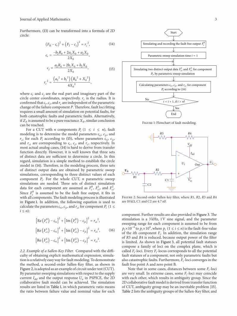
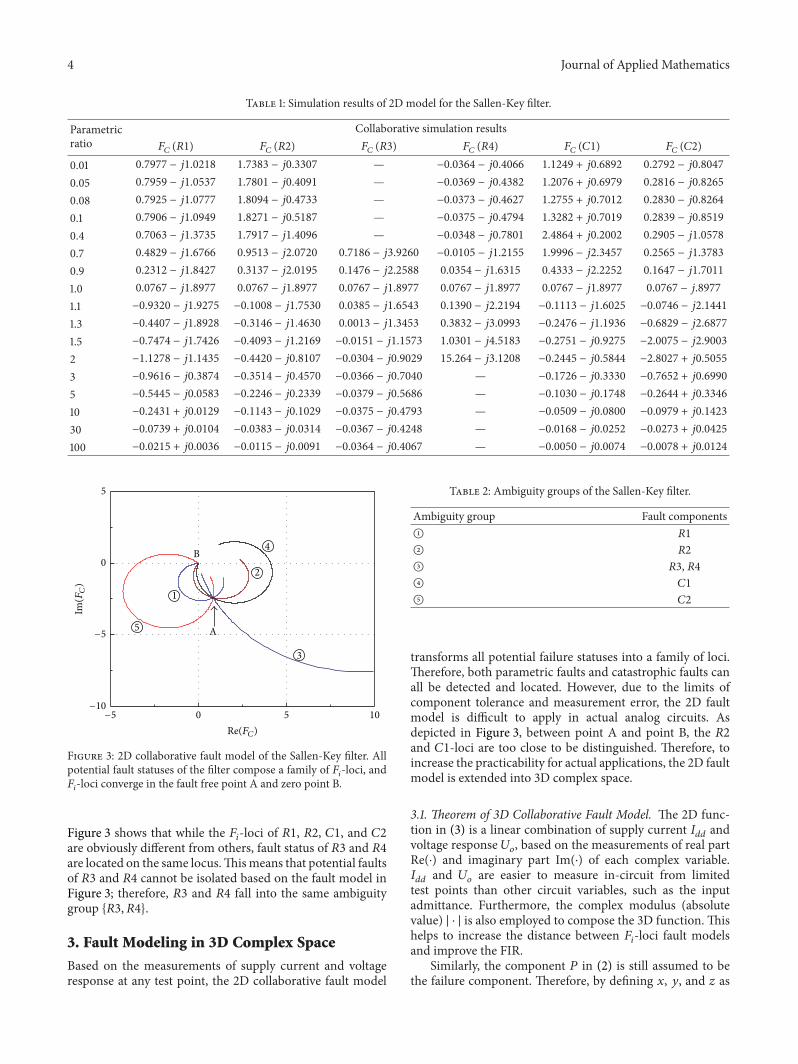
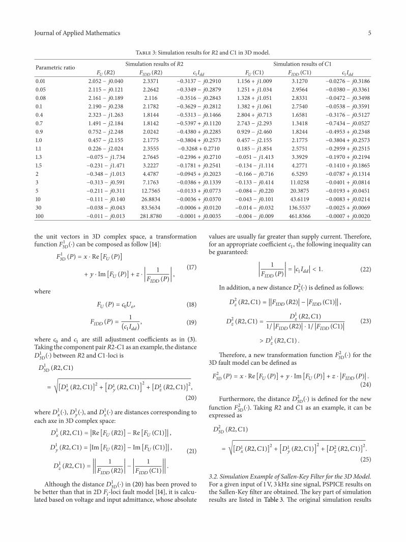
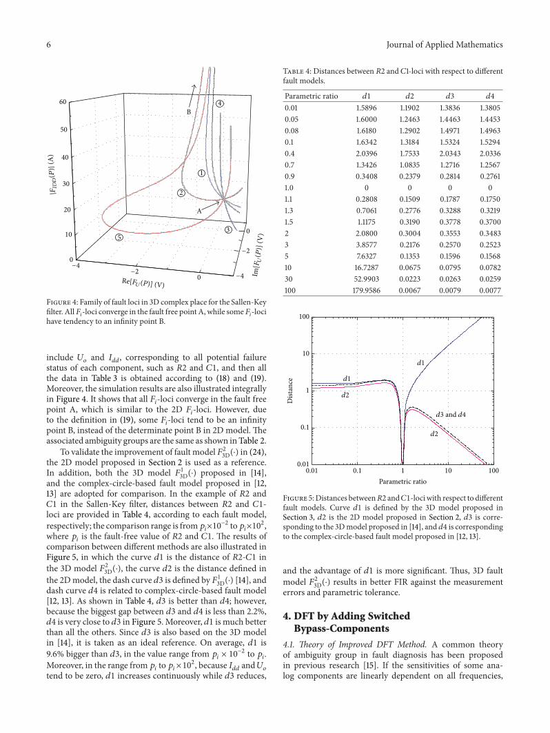
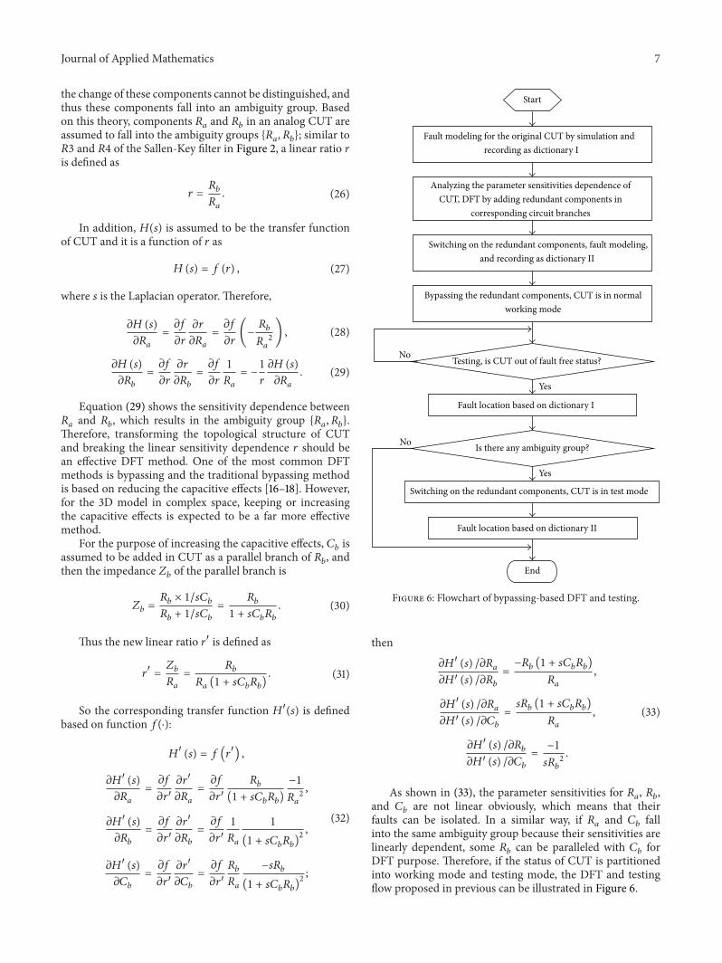
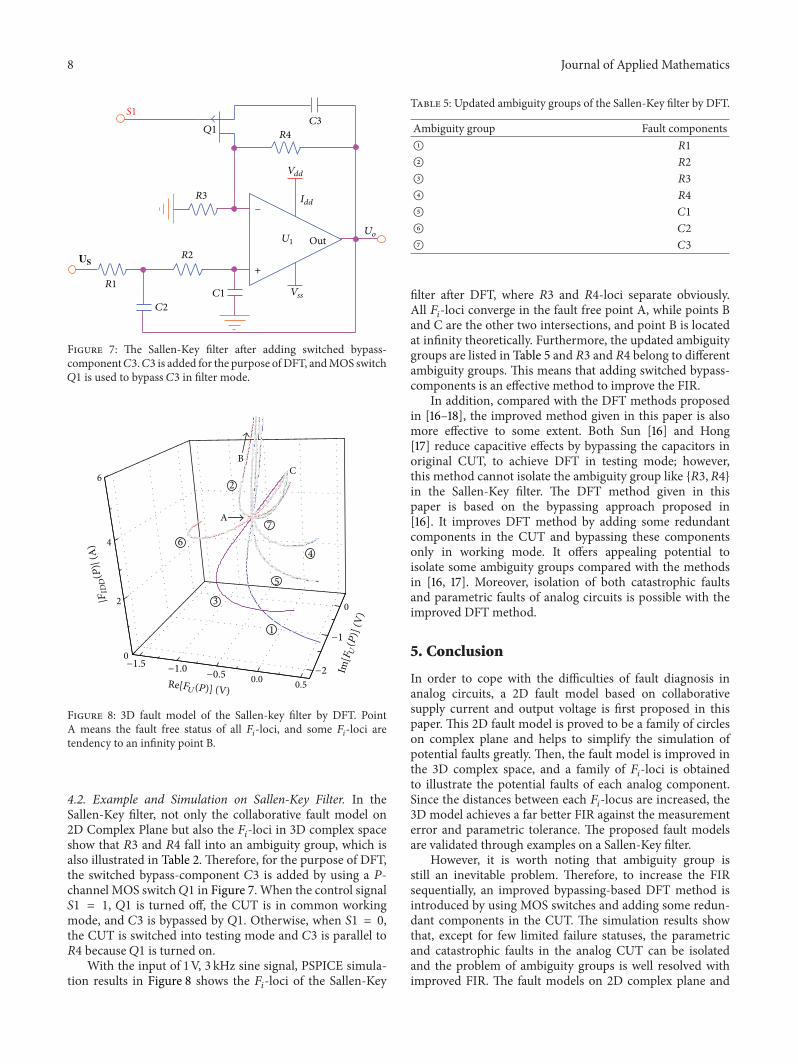