Research Article Impact of Climate Change on Hydrologic ...downloads.hindawi.com/journals/amete/2016/1404290.pdf · hydrologic cycle, such as rainfall, evaporation, runo , and temperature

Research ArticleImpact of Climate Change on Hydrologic Extremes in the UpperBasin of the Yellow River Basin of China

Jun Wang,1 Zhongmin Liang,1,2 Dong Wang,1 Tian Liu,1 and Jing Yang1

1College of Hydrology and Water Resources, Hohai University, Nanjing 210098, China2State Key Laboratory of Hydrology-Water Resources and Hydraulic Engineering, Hohai University, Nanjing 210098, China

Correspondence should be addressed to Zhongmin Liang; [email protected]

Received 16 October 2015; Revised 21 February 2016; Accepted 17 March 2016

Academic Editor: Jingfeng Wang

Copyright © 2016 Jun Wang et al.This is an open access article distributed under theCreativeCommonsAttribution License, whichpermits unrestricted use, distribution, and reproduction in any medium, provided the original work is properly cited.

To reveal the revolution law of hydrologic extremes in the next 50 years and analyze the impact of climate change on hydrologicextremes, the following main works were carried on: firstly, the long duration (15 d, 30 d, and 60 d) rainfall extremes accordingto observed time-series and forecast time-series by dynamical climate model product (BCC-CSM-1.1) were deduced, respectively,on the basis that the quantitative estimation of the impact of climate change on rainfall extremes was conducted; secondly, theSWAT model was used to deduce design flood with the input of design rainfall for the next 50 years. On this basis, quantitativeestimation of the impact of climate change on long duration flood volume extremes was conducted. It indicates that (1) the value oflong duration rainfall extremes for given probabilities (1%, 2%, 5%, and 10%) of the Tangnaihai basin will rise with slight increasingrate from 1% to 6% in the next 50 years and (2) long duration flood volume extremes of given probabilities of the Tangnaihai basinwill rise with slight increasing rate from 1% to 6% in the next 50 years. The conclusions may provide technical supports for basinlevel planning of flood control and hydropower production.

1. Introduction

Climate change has affectedmany fields of nature and humansociety in recent years and has been one of themost attractiveresearch fields. On the background, the estimation andsimulation of the impact of climate change in the hydrologyhave been becoming a research topic. Many hydrologists [1–4], who have done research on the hydrological response toclimate change and human activities, believe that anthro-pogenic global climate change and human activities havesignificantly affected hydrologic cycle and resulted in changesin the spatial and temporal distribution of water resources atboth global and local scales. It is no doubt that the changes inthe hydrological cycle will have serious impacts on ecological,social, and economic situations [5, 6] and bring us severechallenges. To respond to the climate change challenge, one ofthe most important tasks is to reveal influencing mechanismof hydrologic cycle by climate change and to predict theimpact on corresponding fields.Many hydrologists have beenworking on it; for example, some studies have identified

robust trends over some specific regions [7, 8]. However,there are still many questions unclear and the researchshould be continued. With the development of society, thedemand of scientificity of the basin level and national plan-ning of flood control, hydropower production, agriculturalirrigation, and ecosystem preservation are increasing; hence,projecting the future climate and assessing its probableimpact on water resources are critical. Many studies on theimpacts of climate change on hydrological regimes [9–11]have been conducted. In these studies, global climate modelsand hydrologic model were usually used to simulate thechanges in hydrological regimes at watershed scales.

Most of the previous climate change impact assessmentstudies on hydrological processes of Yellow River watershedfocused on the trend of hydrologic elements [12]. However,the assessment study on revolution law of the hydrologicextremes responding to climate change of Yellow Riverbasin is hardly a blank. To reveal the revolution law ofhydrologic extremes and assess the impact of climate changeon hydrologic extremes in the upper Yellow River basin,

Hindawi Publishing CorporationAdvances in MeteorologyVolume 2016, Article ID 1404290, 13 pageshttp://dx.doi.org/10.1155/2016/1404290

2 Advances in Meteorology

the objectives of the paper include (1) evaluation of theimpact of climate change on precipitation extremes of longduration (15 d, 30 d, and 60 d) for given probabilities (1%,2%, 5%, and 10%); (2) evaluation of the impact of climatechange on flood volume extremes of long duration (15 d,30 d, and 60 d) for given probabilities (1%, 2%, 5%, and10%), through hydrologic frequency analysis that deduce thedesign rainfall for the measured phase and the future byrunning distributed hydrological model (SWAT) with theinput condition of design rainfall to deduce the flood volumeextreme of different duration.The paper focuses on revealingthe impact of climate change on the hydrologic extremesof the Tangnaihai basin which locates in the upstream ofYellow River; the main content is as follows: the methodsapplied to study the impact of climate change on hydrologicextreme, including hydrologic frequency analysis method,the bias correction method, and the hydrological model, aredescribed in Section 2. The study area and available dataare then introduced in the Section 3. The results of impactof climate change on hydrologic extremes are presented inSection 4. The conclusions are finally remarked in Section 5.

2. Methodologies

2.1. Frequency Analysis of Precipitation Extremes. To revealthe statistical law of the hydrologic extremes, hydrologictime series analysis and modeling are an effective approach.Obviously, hydrologic frequency analysis is one of mostpopular approaches which are based on time series to analyzethe law of hydrologic extremes [13, 14]. The key of hydrologicfrequency analysis is to determine the probability distribu-tion of extreme. As we known, there are many functions,including extreme value distribution (Gumbel distribution),generalized extreme value distribution (GEV), log-normaldistribution (L-N), the Pearson type III distribution (P-III),and the logarithmic Pierre Johnson III distribution, thatcould be used as the probability distribution of hydrologicextremes.

In China, Liang [15] showed that the P-III distributionis suitable for description of the statistical law of hydrologicextremes, such as annual maximum rainfall, annual max-imum flood peak discharge, and annual maximum floodvolume of different duration, based on the application expe-riences.Therefore, the Pearson type III (P-III) curve has beenused for the hydrologic frequency analysis in China.

The P-III curve is known as the 𝛾 distribution mathe-matically (Gamma distribution with three parameters). Itsprobability density function is expressed as follows:

𝑓 (𝑥) =𝛽𝛼

Γ (𝛼)(𝑥 − 𝑎

0)𝛼−1

𝑒−𝛽(𝑥−𝑎0),

𝑥 > 𝑎0, 𝛼 > 0, 𝛽 > 0,

(1)

where 𝑎0, 𝛽, and 𝛼 denote the position, scale, and shape

parameters of the distribution, respectively. The relation of

these parameters and three moments (𝐸𝑥, 𝐶V, and 𝐶𝑠) canbe expressed as follows:

𝑎0= 𝐸𝑥(1 −

2𝐶V𝐶𝑠) ,

𝛼 =4

𝐶𝑠2,

𝛽 =2

𝐸𝑥𝐶V𝐶𝑠,

(2)

where 𝐸𝑥 denotes the mean of hydrologic extreme timeseries; 𝐶V is the variance of hydrologic extreme time series;and 𝐶𝑠 is the variable coefficient of hydrologic extreme timeseries.

Hydrologic frequency analysis and calculation are toascertain the random variable 𝑥 corresponding to the spec-ified frequency 𝑝, which can be obtained by the distributionfunction defined by transcendental probability:

𝑝 = 𝐹 (𝑥𝑝) = 𝑃 (𝑥 ≥ 𝑥

𝑝) = ∫

∞

𝑥𝑝

𝑓 (𝑥) 𝑑𝑥. (3)

To simplify the integration solution of (3), the variables ofthe Pearson type III distribution can be obtained by standardtransformation of variable 𝑥:

Φ =𝑥 − 𝐸𝑥

𝐸𝑥𝐶V, (4)

where Φ is known as coefficient of mean deviation. Then theintegral operation of 𝑥 is

𝑝 = 𝑃 (Φ ≥ Φ𝑝) = ∫

∞

Φ𝑝

𝑔 (Φ, 𝛼) 𝑑Φ

=𝛼𝛼/2

Γ (𝛼)∫

∞

Φ𝑝

(Φ + √𝛼)𝛼−1

𝑒−√𝛼(Φ+√𝛼)

𝑑Φ,

(5)

where the integrand 𝑔(Φ, 𝛼) contains only one unknownparameter 𝛼 or 𝐶𝑠 (𝛼 = 4/𝐶𝑠2). According to hydrologiccustomary, the relationship of 𝐶𝑠, 𝑝, and Φ

𝑝is tabulated

in advance, namely, Φ-value hydrographic table. The corre-sponding 𝑥

𝑝can be obtained through the inverse transform

of (4) which is expressed as follows:

𝑥𝑝= 𝐸𝑥 (1 + 𝐶VΦ

𝑝) . (6)

2.2. Frequency Analysis of Flood Volume Extremes with Differ-ent Durations. Approach to deduce flood volume extremeswith different durations can be divided into two typesaccording to the data condition [16]: one is the so-calleddirect method when the length of observed discharge timeseries is relatively long. According to observed maximumdischarge time series, the flood volume extremes of differentduration with a certain probability can be deduced byhydrologic frequency analysis as shown in Section 2.1; theother one is the so-called indirect method when the length ofobserved discharge time series is relatively short or there is noobserved discharge data. According to observed precipitation

Advances in Meteorology 3

data, the precipitation extremes of different duration with acertain probability can be deduced by hydrologic frequencyanalysis firstly, on the basis that the flood volume extremeswith different durations of corresponding probability canbe deduced by rainfall-runoff model on the hypothesis thatrainfall with given frequency could generate the flood withthe same frequency.

There are many hydrologic models for rainfall-runoffsimulation; in the paper, the SWAT model which is famousas distributed hydrologic model and widely applied all overthe world was adopted to deduce the flood volume.

2.3. Hydrologic Model: SWAT. To evaluate quantitatively theimpact of climate change on the flood extreme, hydrologicmodel is needed to simulate the flood. There are manyrainfall-runoff models such as Xin’anjiang model, TOP-MODEL, and VIC model. In the paper, SWAT model wasselected because of its powerful hydrological process simu-lation capabilities. Known as a famous distributed hydrologicmodel, SWAT model is a continuous-time, semidistributed,process-based river basin or watershed scale model. SWATmodel was developed to predict the impact of land man-agement practices on water, sediment, and chemical yieldsin agricultural watersheds with varying soils, land use, andmanagement conditions over long period of time [17, 18].Comparing with other hydrologic models, SWAT has twooutstanding features. One is the use of Hydrologic ResponseUnit (HRU), which is divided according to land use, soildistribution, and slope type, as the calculation unit [19].SWAT divides a watershed into subbasins. Each subbasinis connected through a stream channel and further eachsubbasin is divided into HRUs. SWAT simulates hydrologyand sediment at the HRU level. Water and sediment fromeach HRU are summarized in each subbasin and then routedthrough the stream network to the watershed outlet [18, 20].The other one is the simulation of surface runoff by using themodified SCS curve number which is deduced based on landuse and soil type of watershed [21].

2.4. Bias Correction of Climate Model. Systematic errors ofclimate models may lead to unrealistic hydrological simula-tions of river flow [22, 23]; thus, bias correctionmethodsmustbe implemented to correct the climate product before appli-cation and analysis. For adjusting climate model product, thelinear scaling, local intensity scaling, power transformation,variance scaling, distribution transfer, and the delta-changeapproaches are the commonly used bias correction methods[24]. Bias correction methods are based on the assumptionthat the same correction algorithm applies to both currentand future climate conditions. In the study, linear scalingmethod was employed to correct the daily precipitation andmonthly precipitation of climate model.

Based on the precipitation simulated by climate modeland the corresponding measured precipitation, correctioncoefficients of each month were calculated. The precipitationpredicted by climate model was modified on the basis ofcorrection coefficients scaling monthly precipitation data

predicted by the model. The correction coefficient can becalculated by

𝜆𝑖=𝑃𝑜

𝑖

𝑃𝑖

, (7)

where 𝜆𝑖is the correction coefficient of the 𝑖th month, 𝑃𝑜

𝑖is

the measured monthly mean precipitation of the 𝑖th monthof reference period, and 𝑃

𝑖is the monthly mean precipitation

simulated by the climate model of the 𝑖th month of referenceperiod.

3. Study Area and Base Data

3.1. Study Area. Tangnaihai basin with a drainage area of122,000 km2 is located in the upstream of Yellow River in thewestern China, accounting for 15% of that of the Yellow Riverbasin. Annual average runoff amount at the Tangnaihai crosssection is 205.2 × 108m3, accounting for 40% of annual meanrunoff amount of YellowRiver basin. It is a semihumid regionwith good vegetation and less human activity. In the study,nine meteorological stations and seven hydrologic stationsare involved. Figure 1 shows the location of the study area andgauging stations distribution.

3.2. Base Data. Five types of data, including hydrometeo-rology data, DEM, land use, soil distribution, and climatemodel data, are involved in the study. The details of data areas follows.

3.2.1. Hydrometeorology Data. Hydrometeorology data usedin the study is the information of the elements influencinghydrologic cycle, such as rainfall, evaporation, runoff, andtemperature. The basic data mainly comes from two sources:one is the 9 meteorological stations mentioned above whichcan provide precipitation, temperature, wind speed, solarradiation, relative humidity, and some other meteorologicaldata; the other one is 7 hydrologic stations shown in Figure 2which can provide precipitation, discharge, and evaporation.The length of the data series ranging from 1960 to 2012 is 53years.

3.2.2. DEM. DEM is the basis for generating digital water-shed system of Tangnaihai basin; in the paper, SRTM (ShuttleRadar Topography Mission) DEM with 90m × 90m reso-lution ratio, which is produced by NASA and NIMA, wasutilized.

3.2.3. Land Use and Soil Distribution. Land use and soildistributionwhich are used to divide the whole basin into dif-ferent HRUs are the basis of runoff yield calculation of SWATmodel and play an important role in hydrologic model struc-ture. In the paper, the dataset ofWESTDC Land Cover V.1.0investigated byChineseAcademy of Sciences with the scale of1 : 100,000 and the soil distribution data provided by Instituteof Soil Science from the second national land survey werechosen to build SWAT model.


(

Zeku

DariMaqu

Henan

Maduo

Jimai

Guoluo

Tongde

JiuzhiDashui

Tangke

Xinghai

Jungong

Hongyuan

Ruoergai

Huangyan

Tangnaihai

China Yellow River watershed

Tangnaihai basin

StationOutletRiver

N

Figure 1: Location and hydrometeorological stations of the study area.

3.2.4. Climate Model Product. There are many dynamicalclimatemodel products under different climate scenarios andhypothesis released by IPCCAR5. It is unnecessary and unre-alistic to analyze every climate model product in this study;one certain climate model product should be focused oninstead. In this paper, several climate model products whichsuit the region where China locates were selected firstly.On the basis, the accuracy of predicted precipitation of theclimate model products was analyzed, and the climate modelproduct called BCC-CSM-1.1 is of good prediction effect andchosen as the basic data for conducting the evolution law ofhydrologic extreme value of the upstream region of YellowRiver basin. BCC-CSM-1.1 is provided by Beijing ClimateCenter of China Meteorological Administration with a spaceresolution 1.125∘ × 1.125∘.

3.3. Durations of Hydrologic Selection. The longer durations(15 d, 30 d, and 60 d), instead of shorter durations (1 d,

3 d, 5 d, or 7 d), of hydrologic extreme were focused onin the paper. There are two reasons. First, flood volume oflonger duration plays a control role in flood control theconsequences for larger basin. The Tangnaihai basin is alarge basin with drainage area of 122,000 km2 and its basinflow concentration time is >15 d. From this view, research onflood extreme of longer durations might be more meaningfulfor Tangnaihai basin; second, there are many reservoirsbuilt or planned to be built, and flood volume of shorterdurations will be influenced greatly by reservoir regulation,while that of longer durations will be maintain natural.Therefore, the time series of flood volumeof shorter durations(1 d, 3 d, 5 d, or 7 d) are inconsistent and not suitable forfrequency analysis of which theory is built on consistency oftime series. In conclusion, evaluation the impact of climatechange on hydrologic extreme of longer durations (15 d,30 d, and 60 d) would be more meaningful and applica-tive.


0.020.040.060.080.0

100.0120.0140.0160.0

1960

/1

1965

/1

1970

/1

1975

/1

1980

/1

1985

/1

1990

/1

1995

/1

2000

/1

2005

/1

Prec

ipita

tion

(mm

)

Time (d)Modified precipitationObserved precipitation

Figure 2: Results of precipitation correction (1960–2006) of theTangnaihai basin.

4. Results and Discussion

To reveal the revolution law of hydrologic extremes of theTangnaihai basin, the observed hydrologic time series from1960 to 2010 and the predicted precipitation time series from2011 to 2060 were used. In this paper, the years from 1960 to2010 are defined as the measured phase while the years from2011 to 2060 are denoted as the next 50 years.

4.1. Bias Correction of BCC-CSM-1.1. To correct systematicerrors of simulated precipitation of BCC-CSM-1.1 of theTangnaihai basin, the correction model was built with linearregression relationship between observed and simulated pre-cipitation in synchronized period. In the paper, the precipita-tion time series range from 1960 to 2006. Figure 2 shows thecorrection results.

According to the correction results, it is found that therewas large correction error in themonths of low-water seasonsas the position of black circle shows in Figure 2, while therest of correction results were of high accuracy. Since thepaper focused on studying the precipitation extreme, theerror of low-watermonthswill have little effect.Therefore, thecorrection model built can be used to correct the simulationprecipitation of BCC-CSM-1.1 of the Tangnaihai basin.

4.2. Impact of Climate Change on Rainfall Extremes

4.2.1. Rainfall Extremes of Different Duration Analysis Basedon Observed Data. The statistical law of rainfall extremes inthe measured phase should be revealed first for uncoveringthe influences of climate on rainfall extremes. In the paper,the series of maximum value of annual rainfall extremes indifferent durations, such as 15 days, 30 days, and 60 days,was calculated by observed data and utilized to invest thestatistical law of rainfall extremes. Asmentioned above, the P-III distribution is suited for frequency analysis of hydrologicextremes in China. Therefore, the design rainfall of differentdurations (15 d, 30 d, and 60 d) of any probability can bededuced. Figure 3 shows the frequency curve of rainfall ofdifferent durations fitting by observed data. The parameters

Table 1: Results of parameters estimation of P-III distribution forthe measured phase.

Duration (d) Mean (mm) 𝐶V 𝐶𝑠/𝐶V15 80 0.20 3.530 130 0.19 3.560 215 0.17 3.5

Table 2: Design rainfall in different durations of different returnperiods for the measured phase (mm).

Duration (d) Return period (a)100 50 20 10

15 126 119 110 10230 200 190 175 16360 316 302 281 264

0

40

80

120

160

200

240

280

320

360

400

440Pr

ecip

itatio

n (m

m)

0 0.01 1 10 40 70 95 99.5

Probability (%)

15-day maximum precipitation

60-day maximum precipitation30-day maximum precipitation

Frequency curve of 15-day maximum precipitationFrequency curve of 30-day maximum precipitationFrequency curve of 60-day maximum precipitation

Figure 3: Frequency curve-fitting of rainfall extreme in differentdurations for the measured phase of Tangnaihai basin.

estimation results of P-III distribution are listed in Table 1while the design values for given probabilities are listed inTable 2.

4.2.2. Analysis of Rainfall Extremes of Different Durations withBCC-CSM-1.1. Time series of rainfall extremes in differentdurations (15 d, 30 d, and 60 d) in the next 50 years from 2011to 2060 can be extracted according to the correction results ofBCC-CSM-1.1. Similar to frequency analysis in the measuredphase, the parameters estimation of P-III distribution anddesign value of different durations for next 50 years can beobtained. The corresponding frequency curves are shown inFigure 4, and the parameters estimation results are listed inTable 3 while the design values of several given probabilitiesare listed in Table 4.


Table 3: Results of parameters estimation of P-III distribution forthe next 50 years.

Duration (d) Mean (mm) 𝐶V 𝐶𝑠/𝐶V15 84 0.18 3.530 137 0.17 3.560 231 0.15 3.5

Table 4: Design rainfall in different durations of different returnperiod for the next 50 years (mm).


15 128 122 113 10530 201 192 179 16860 332 318 297 280

0

40

80

120

160

200

240

280

320

360

400

440

Prec

ipita

tion

(mm

)

0 0.01 1 10 40 70 95 99.5

Probability (%)

15-day maximum precipitation

60-day maximum precipitation30-day maximum precipitation

Frequency curve of 15-day maximum precipitationFrequency curve of 30-day maximum precipitationFrequency curve of 60-day maximum precipitation

Figure 4: The frequency curves of 15-day, 30-day, and 60-daymaximum rainfall of Tangnaihai basin for the next 50 years.

4.2.3. Discussion about the Impact of ClimateChange on Rainfall Extremes

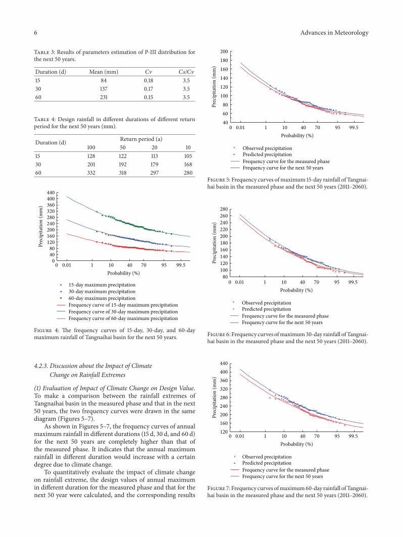
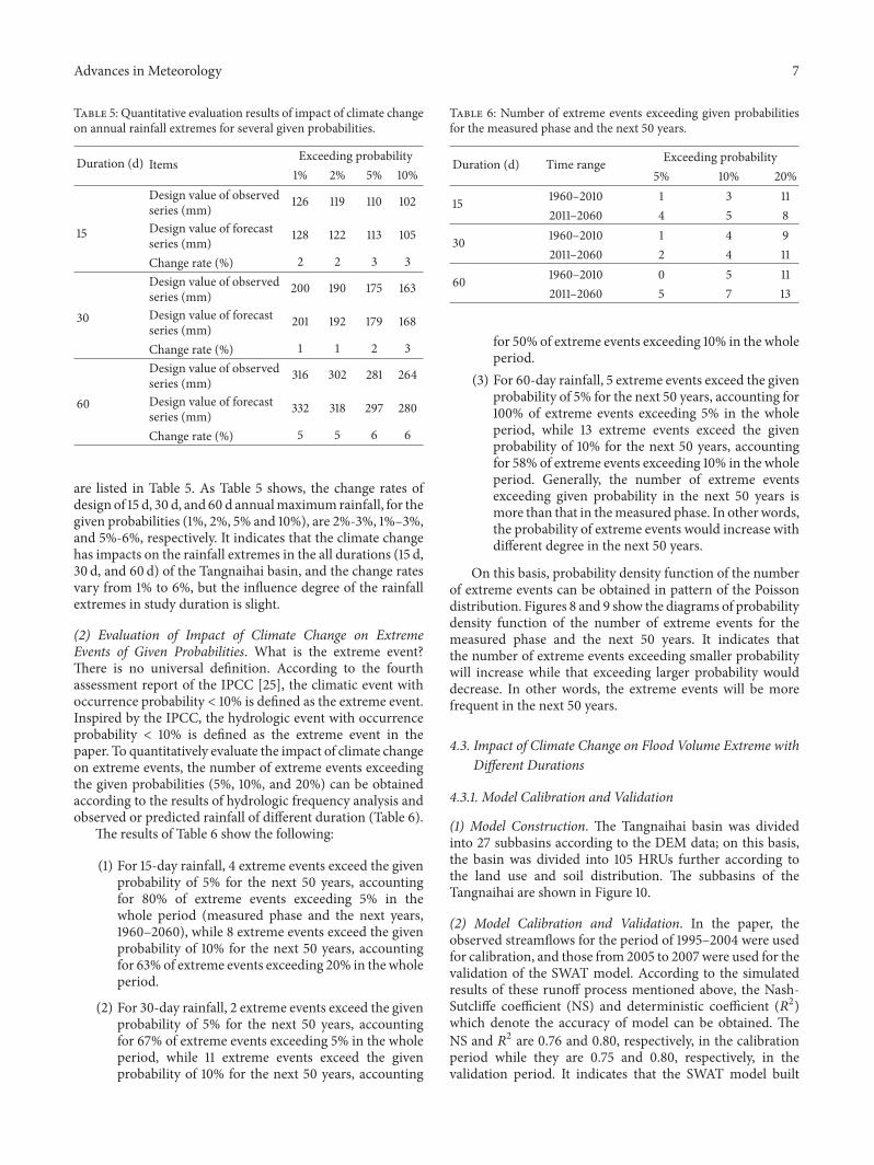
(1) Evaluation of Impact of Climate Change on Design Value.To make a comparison between the rainfall extremes ofTangnaihai basin in the measured phase and that in the next50 years, the two frequency curves were drawn in the samediagram (Figures 5–7).

As shown in Figures 5–7, the frequency curves of annualmaximum rainfall in different durations (15 d, 30 d, and 60 d)for the next 50 years are completely higher than that ofthe measured phase. It indicates that the annual maximumrainfall in different duration would increase with a certaindegree due to climate change.

To quantitatively evaluate the impact of climate changeon rainfall extreme, the design values of annual maximumin different duration for the measured phase and that for thenext 50 year were calculated, and the corresponding results

Prec

ipita

tion

(mm

)

0 0.01 1 10 40 70 95 99.5

Probability (%)

Observed precipitationPredicted precipitationFrequency curve for the measured phaseFrequency curve for the next 50 years

40

60

80

100

120

140

160

180

200

Figure 5: Frequency curves ofmaximum 15-day rainfall of Tangnai-hai basin in the measured phase and the next 50 years (2011–2060).

Prec

ipita

tion

(mm

)

0 0.01 1 10 40 70 95 99.5

Probability (%)


80

100

120

140

160

180

200

220

240

260

280

Figure 6: Frequency curves ofmaximum30-day rainfall of Tangnai-hai basin in the measured phase and the next 50 years (2011–2060).

120

160

200

240

280

320

360

400

440

Prec

ipita

tion

(mm

)

0 0.01 1 10 40 70 95 99.5

Probability (%)


Figure 7: Frequency curves ofmaximum60-day rainfall of Tangnai-hai basin in the measured phase and the next 50 years (2011–2060).


Table 5: Quantitative evaluation results of impact of climate changeon annual rainfall extremes for several given probabilities.

Duration (d) Items Exceeding probability1% 2% 5% 10%

15

Design value of observedseries (mm) 126 119 110 102

Design value of forecastseries (mm) 128 122 113 105

Change rate (%) 2 2 3 3

30




60




are listed in Table 5. As Table 5 shows, the change rates ofdesign of 15 d, 30 d, and 60 d annualmaximumrainfall, for thegiven probabilities (1%, 2%, 5% and 10%), are 2%-3%, 1%–3%,and 5%-6%, respectively. It indicates that the climate changehas impacts on the rainfall extremes in the all durations (15 d,30 d, and 60 d) of the Tangnaihai basin, and the change ratesvary from 1% to 6%, but the influence degree of the rainfallextremes in study duration is slight.

(2) Evaluation of Impact of Climate Change on ExtremeEvents of Given Probabilities. What is the extreme event?There is no universal definition. According to the fourthassessment report of the IPCC [25], the climatic event withoccurrence probability < 10% is defined as the extreme event.Inspired by the IPCC, the hydrologic event with occurrenceprobability < 10% is defined as the extreme event in thepaper. To quantitatively evaluate the impact of climate changeon extreme events, the number of extreme events exceedingthe given probabilities (5%, 10%, and 20%) can be obtainedaccording to the results of hydrologic frequency analysis andobserved or predicted rainfall of different duration (Table 6).

The results of Table 6 show the following:

(1) For 15-day rainfall, 4 extreme events exceed the givenprobability of 5% for the next 50 years, accountingfor 80% of extreme events exceeding 5% in thewhole period (measured phase and the next years,1960–2060), while 8 extreme events exceed the givenprobability of 10% for the next 50 years, accountingfor 63% of extreme events exceeding 20% in thewholeperiod.

(2) For 30-day rainfall, 2 extreme events exceed the givenprobability of 5% for the next 50 years, accountingfor 67% of extreme events exceeding 5% in the wholeperiod, while 11 extreme events exceed the givenprobability of 10% for the next 50 years, accounting

Table 6: Number of extreme events exceeding given probabilitiesfor the measured phase and the next 50 years.

Duration (d) Time range Exceeding probability5% 10% 20%

15 1960–2010 1 3 112011–2060 4 5 8

30 1960–2010 1 4 92011–2060 2 4 11

60 1960–2010 0 5 112011–2060 5 7 13

for 50% of extreme events exceeding 10% in the wholeperiod.

(3) For 60-day rainfall, 5 extreme events exceed the givenprobability of 5% for the next 50 years, accounting for100% of extreme events exceeding 5% in the wholeperiod, while 13 extreme events exceed the givenprobability of 10% for the next 50 years, accountingfor 58% of extreme events exceeding 10% in the wholeperiod. Generally, the number of extreme eventsexceeding given probability in the next 50 years ismore than that in themeasured phase. In other words,the probability of extreme events would increase withdifferent degree in the next 50 years.

On this basis, probability density function of the numberof extreme events can be obtained in pattern of the Poissondistribution. Figures 8 and 9 show the diagrams of probabilitydensity function of the number of extreme events for themeasured phase and the next 50 years. It indicates thatthe number of extreme events exceeding smaller probabilitywill increase while that exceeding larger probability woulddecrease. In other words, the extreme events will be morefrequent in the next 50 years.

4.3. Impact of Climate Change on Flood Volume Extreme withDifferent Durations

4.3.1. Model Calibration and Validation

(1) Model Construction. The Tangnaihai basin was dividedinto 27 subbasins according to the DEM data; on this basis,the basin was divided into 105 HRUs further according tothe land use and soil distribution. The subbasins of theTangnaihai are shown in Figure 10.

(2) Model Calibration and Validation. In the paper, theobserved streamflows for the period of 1995–2004 were usedfor calibration, and those from 2005 to 2007 were used for thevalidation of the SWAT model. According to the simulatedresults of these runoff process mentioned above, the Nash-Sutcliffe coefficient (NS) and deterministic coefficient (𝑅2)which denote the accuracy of model can be obtained. TheNS and 𝑅2 are 0.76 and 0.80, respectively, in the calibrationperiod while they are 0.75 and 0.80, respectively, in thevalidation period. It indicates that the SWAT model built


0 1 20

0.2

0.4

0.6

0.8

1PD

F

0

0.2

0.4

0.6

0.8

1

PDF

0 1 2Number of occurrencesNumber of occurrences

PDF for 1960–2010PDF for 1960–2010

PDF for 1960–2010PDF for 1960–2010

0

0.2

0.4

0.6

0.8

1

PDF

0 1 2Number of occurrences

PDF for 1960–2010PDF for 1960–2010

15d 30d

60d

Figure 8: Probability density diagram of the precipitation exceeding probability of 5% for the measured phase and the next 50 years of theTangnaihai basin.

is of good accuracy and can be adopted to simulate therainfall-runoff in the study area. Taking several runoff pro-cesses as an example, Figures 11 and 12 show the simulationresults.

4.3.2. Design Rainfall in Different Durations Deduced for Next50 Years. Long duration rainfall extremes of certain givenprobabilities (1%, 2%, 5%, and 10%) of the Tangnaihai basinfor the next 50 years were deduced in Section 4.2.2. However,the results are not enough to meet the requirements fordeducing long duration flood volume extremes by SWAT,

and the design rainfall process is also needed. Therefore, thedesign rainfall process should be deduced firstly.

The basic idea and procedure to deduce design rainfallprocess in different given probabilities are as follows: (1)selecting one typical storm process with certain principles;(2) magnifying it according to the design rainfall valueand keeping the maximum rainfall of given duration andprobability of magnified typical storm process equal to thedesign rainfall of corresponding duration and probability. Inthe paper, the storm process that occurred from 28/5/1989to 26/7/1989 was selected as the typical storm. According to


0 1 2 3 40

0.2

0.4

0.6

0.8

PDF

PDF for 1960−2010PDF for the next 50 years

Number of occurrences0 1 2 3 4

0

0.2

0.4

0.6

0.8

PDF


Number of occurrences

0 1 2 3 40

0.2

0.4

0.6

0.8

PDF


Number of occurrences

15d 30d

60d

Figure 9: Probability density diagram of the rainfall extreme event exceeding probability of 20% for the measured phase and the next 50years of Tangnaihai basin.

the magnified method, design rainfall process of differentreturn periods (100 a, 50 a, 20 a, and 10 a) can be obtained.Taking return period of 100 a as an example, Figure 13 showsthe process of rainfall.

Similarly, design rainfall process of different return peri-ods (100 a, 50 a, 20 a, and 10 a) for the measured phase canbe obtained. Taking return period of 100 a as an example,Figure 14 shows the process of rainfall.

4.3.3. Design Flood Volume in Different Durations Deducedfor Next 50 Years. According to the design rainfall process

of given probability, the flood hydrography of correspondingprobability was deduced, respectively, by running the SWAT.On this basis, the long duration flood volume of differentprobabilities for the next 50 years can be obtained.The resultsare listed in Table 7.

4.3.4. Discussion on Impact of Climate Change on Flood Vol-ume Extreme. Taking the design rainfall process in differentprobability as input condition for SWAT, the design floodprocess in corresponding probability can be obtained byrunning the model. In the paper, design flood process of


Tangnaihai

26

5

9

310

15

25

4

14

6

7

11

27

18

1312

22

8

17

23

20

16 2421

19

12

OutletRiverSubbasin

Figure 10: Subbasins of Tangnaihai basin.

Table 7: Long duration flood volume of different probabilities forthe next 50 years of Tangnaihai basin.


15 126 119 110 10230 200 190 175 16360 316 302 281 264

Table 8: Change rates of design flood volume in different durationsof given probabilities (%).


15 3 3 3 130 3 2 3 160 3 5 6 5

different return period including 100 a, 50 a, 20 a, and 10 a wassimulated. Figures 15–18 show the design hydrographs whichare of four return periods (100 a, 50 a, 20 a, and 10 a) for themeasured phase and the next 50 years, respectively.

According to Figures 15–18, it is obvious that the designflood hydrograph is higher for the next 50 years than thatof the measured phase. It indicates that the flood volumeextremes show an increasing trend in the Tangnaihai basin.To take a close investigation into the rising trend and makea quantitative estimation, change rates of flood volume indifferent durations of four kinds of probabilities (1%, 2%, 5%,and 10%) are calculated and listed in Table 8.

0

500

1000

1500

2000

2500

3000

1/1/

1995

1/1/

1996

1/1/

1997

1/1/

1998

1/1/

1999

1/1/

2000

1/1/

2001

1/1/

2002

1/1/

2003

Time (d)

Simulated dischargeObserved discharge

Disc

harg

e (m

3/s

)

Figure 11: Observed and simulated hydrographs of Tangnaihai crosssection in calibration period.

According to Table 8, the increasing rates of 15-day floodvolume for different return period vary from 1% to 3%;the increasing rates of 30-day flood volume for differentreturn period vary from 1% to 3%; and the increasing ratesof 60-day flood volume for different return period varyfrom 3% to 6%. It indicates that the increasing rates oflong duration flood volume of Tangnaihai basin is less than10%. In other words, the flood volume extremes in longduration of Tangnaihai basin increase slightly in the next 50years.


0

500

1000

1500

2000

2500

30001/

1/20

05

1/1/

2006

1/1/

2007

Time (d)

Simulated dischargeObserved discharge

Disc

harg

e (m

3/s

)

Figure 12: Observed and simulated hydrographs of Tangnaihaicross section in validation period.

02468

101214

16

1 6 11 16 21 26 31 36 41 46 51 56

Prec

ipita

tion

(mm

)

Time (d)

Figure 13: The process of 100-year design rainfall of Tangnaihaibasin for the next 50 years.

5. Conclusions

To study the impact of climate change on hydrologic extremesin the Tangnaihai basin which locates in the upstream ofYellow River, the BCC-CSM-1.1 released by IPCC 5 wasused to forecast rainfall in the next 50 years (2011–2060).On this basis, according to the observed hydrologic dataseries, the evolution law of long duration hydrologic extremesof Tangnaihai basin is revealed. Main conclusions can beachieved as follows.

(1) It indicates that the values of long duration (15 d, 30 d,and 60 d) rainfall extremes of Tangnaihai basin willrise by slightly increasing rate in the next 50 years.According to analysis results of rainfall extremes indifferent durations, 15-day design rainfall of givenprobabilities (1%, 2%, 5%, and 10%) will increase by2%-3%; similarly, 30-day design rainfall will increaseby 1%–3% and 60-day design rainfall will increase by5%-6%, respectively. It is obvious that the increasingrates of rainfall extremes in given probabilities are lessthan 10%; in other words, the rainfall extremes of theTangnaihai basin would increase with a slight degree.

02468

101214

1 6 11 16 21 26 31 36 41 46 51 56

Prec

ipita

tion

(mm

)

Time (d)

Figure 14: The process of 100-year design rainfall of Tangnaihaibasin for the measured phase.

0500

10001500200025003000350040004500

0 5 10 15 20 25 30 35 40 45 50 55 60Time (d)

Measured phaseNext 50 years

Disc

harg

e (m

3/s

)

Figure 15: 100-year flood hydrograph for the measured phase andthe next 50 years of Tangnaihai basin.

(2) It indicates that the number of extreme events exceed-ing smaller probability will increase for the next 50years. According to the analysis of number of extremeevents exceeding given probability, it is obvious thatthe extreme events of long duration rainfall exceedinggiven probabilities (5%, 10%, and 20%) will get morefrequent.

(3) It indicates that the values of long duration (15 d,30 d, and 60 d) flood volume extremes of Tangnaihaibasin will rise by slightly increasing rate in the next50 years. On the hypothesis that rainfall of givenfrequency could generate the flood of the samefrequency, SWAT model was used to deduce designflood with the import of design rainfall for the next50 years, and the long flood volume extremes wereachieved. According to the analysis of results of floodvolume extremes in different duration, 15-day designflood volume of given probabilities (1%, 2%, 5%, and10%) is increasing by 1%–3% based on BCC-CSM-1.1;similarly, 30-day design flood volume is increasing by1%–3% and 60-day design flood volume is increasingby 3%–6%, respectively. It obvious that the increasingrate of flood volume extremes in given probabilityis less than 10%, in other words, the flood volume


0500

10001500200025003000350040004500

0 5 10 15 20 25 30 35 40 45 50 55 60Time (d)

Next 50 yearsMeasured phase

Disc

harg

e (m

3/s

)

Figure 16: 50-year flood hydrograph for the measured phase andthe next 50 years of Tangnaihai basin.

0500

1000150020002500

35003000

45004000

0 5 10 15 20 25 30 35 40 45 50 55 60Time (d)


Disc

harg

e (m

3/s

)

Figure 17: 20-year flood hydrograph for themeasured phase and thenext 50 years of Tangnaihai basin.

extremes of the Tangnaihai basin would increase witha slight degree.

Generally, the long duration hydrologic extremes of theTangnaihai basin in Yellow River basin would increase bya slight degree in the next 50 years. The conclusions wereaddressed on the basis of BCC-CSM-1.1. However, if severalmore suitable climate change model products were adopted,the conclusions on impact of climate change in study area willbemore reliable. To improve the study, wewill trymoreGCMoutputs and continue in-depth studies on the same theme inthe future.

Competing Interests

The authors declare that there are no competing interestsregarding the publication of this paper.

Authors’ Contributions

The studies were designed by Jun Wang, Zhongmin Liang,Dong Wang, Tian Liu, and Jing Yang. Specifically, Jun Wang

0

500

1000

1500

2000

2500

3000

0 5 10 15 20 25 30 35 40 45 50 55 60Time (d)


Disc

harg

e (m

3/s

)

Figure 18: 10-year flood hydrograph for themeasured phase and thenext 50 years of Tangnaihai basin.

and Zhongmin Liang performed the studies and analyzed thedata, Dong Wang processed the precipitation simulated byclimatemodel, Tian Liu built the SWATmodel and calculateddesign flood, and Jing Yang helped to hydrologic frequencyanalysis and helped refine the charts and polish the paper.

Acknowledgments

This study was supported by the Public Welfare IndustrySpecial Fund Project of Ministry of Water Resources ofChina (nos. 201301066 and 201401034), the National NaturalScience Foundation of China (nos. 51109054, 51179046, and51479061), National Science and Technology Support Plan(no. 2013BAB06B01), and Excellent Ph.D. Training program(no. 2015B05514).

References

[1] N. S. Christensen, A.W.Wood,N. Voisin, D. P. Lettenmaier, andR. N. Palmer, “The effects of climate change on the hydrologyand water resources of the Colorado River basin,” ClimaticChange, vol. 62, no. 1–3, pp. 337–363, 2004.

[2] M. K. Jha and P. W. Gassman, “Changes in hydrology andstreamflow as predicted by a modelling experiment forced withclimate models,”Hydrological Processes, vol. 28, no. 5, pp. 2772–2781, 2014.

[3] C. Yang, Z. Yu, Z. Hao, J. Zhang, and J. Zhu, “Impact of climatechange on flood and drought events in Huaihe River Basin,China,” Hydrology Research, vol. 43, no. 1-2, pp. 14–22, 2012.

[4] Z. Yu, T. Yang, and F. W. Schwartz, “Water issues and prospectsfor hydrological science in China,”Water Science and Engineer-ing, vol. 7, no. 1, pp. 1–4, 2014.

[5] A. C. Horrevoets, H. H. G. Savenije, J. N. Schuurman, and S.Graas, “The influence of river discharge on tidal damping inalluvial estuaries,” Journal of Hydrology, vol. 294, no. 4, pp. 213–228, 2004.

[6] N. L. Poff, J. D. Allan,M. B. Bain et al., “The natural flow regime:a paradigm for river conservation and restoration,” BioScience,vol. 47, no. 11, pp. 769–784, 1997.


[7] N. Y. Krakauer and I. Fung, “Mapping and attribution of changein streamflow in the coterminous United States,”Hydrology andEarth System Sciences, vol. 12, no. 4, pp. 1111–1120, 2008.

[8] K. Stahl, H. Hisdal, J. Hannaford et al., “Streamflow trends inEurope: evidence from a dataset of near-natural catchments,”Hydrology and Earth System Sciences, vol. 14, no. 12, pp. 2367–2382, 2010.

[9] F. H. S. Chiew, J. Teng, J. Vaze et al., “Estimating climate changeimpact on runoff across southeast Australia: method, results,and implications of the modeling method,” Water ResourcesResearch, vol. 45, no. 10, Article IDW10414, 2009.

[10] A. Senatore, G. Mendicino, G. Smiatek, and H. Kunstmann,“Regional climate change projections and hydrological impactanalysis for a Mediterranean basin in Southern Italy,” Journal ofHydrology, vol. 399, no. 1-2, pp. 70–92, 2011.

[11] M. V. Shabalova, W. P. A. Van Deursen, and T. A. Buishand,“Assessing future discharge of the river Rhine using regionalclimate model integrations and a hydrological model,” ClimateResearch, vol. 23, no. 3, pp. 233–246, 2003.

[12] Q. Liu and B. Cui, “Impacts of climate change/variability onthe streamflow in the Yellow River Basin, China,” EcologicalModelling, vol. 222, no. 2, pp. 268–274, 2011.

[13] C. Cunnane, “Statistical distribution for flood frequency analy-sis,” Operational Hydrology Report (WMO) 781, 1989.

[14] D. R. Maidment, Handbook of Hydrology, McGraw-Hill, NewYork, NY, USA, 1992.

[15] Z. M. Liang, Hydrologic Analysis and Calculation, China WaterPower Press, 2013.

[16] Y. F. Chen, Ed., Engineering Hydrology and Flood ControlCalculation andWater Resources Analysis, ChinaWater&PowerPress, 2013.

[17] J. G. Arnold, R. Srinivasan, R. S. Muttiah, and J. R. Williams,“Large area hydrologic modeling and assessment part I: modeldevelopment,” Journal of the American Water Resources Associ-ation, vol. 34, no. 1, pp. 73–89, 1998.

[18] S. L. Neitsch, J. G. Arnold, J. R. Kiniry, and J. R.Williams, SWATUser Manual, Version 2005, Grassland Soil and Water ResearchLaboratory, Temple, Tex, USA, 2005.

[19] J. G. Arnold, J. R. Kiniry, R. Srinivasan, J. R. Williams, E.B. Haney, and S. L. Neitsch, SWAT Input/Output File Docu-mentation, Version 2009, Grassland Soil and Water ResearchLaboratory, Temple, Tex, USA, 2011.

[20] S. L. Neitsch, J. G. Arnold, J. R. Kiniry, and J. R. Williams,“SWAT user manual, version 2009,” Texas Water ResourcesInstitute Technical Report, Texas A&M University, CollegeStation, Tex, USA, 2011.

[21] USDA Soil Conservation Service, National Engineering Hand-book. Hydrology Section 4, chapter 4–10, 1972.

[22] S. Bergstrom, B. Carlsson, M. Gardelin, G. Lindstrom, A.Pettersson, and M. Rummukainen, “Climate change impactson runoff in Sweden assessments by global climate models,dynamical down-scaling and hydrological modelling,” ClimateResearch, vol. 16, pp. 101–112, 2001.

[23] L. P. Graham, J. Andreaasson, and B. Carlsson, “Assessingclimate change impacts on hydrology from an ensemble ofregional climate models, model scales and linking methods—a case study on the Lule River basin,” Climatic Change, vol. 81,no. 1, pp. 293–307, 2007.

[24] C. Teutschbein and J. Seibert, “Bias correction of regionalclimate model simulations for hydrological climate-changeimpact studies: review and evaluation of different methods,”Journal of Hydrology, vol. 456-457, pp. 12–29, 2012.

[25] IPCC, Climate Change 2007: The Physical Basis. Contributionof Working Group1 to the Fouth Assessment Report of the IPCC,Cambridge University Press, New York, NY, USA, 2007.

Submit your manuscripts athttp://www.hindawi.com

Hindawi Publishing Corporationhttp://www.hindawi.com Volume 2014

ClimatologyJournal of

EcologyInternational Journal of


EarthquakesJournal of


Hindawi Publishing Corporationhttp://www.hindawi.com

Applied &EnvironmentalSoil Science

Volume 2014

Mining


Journal of

Hindawi Publishing Corporation http://www.hindawi.com Volume 2014

International Journal of

Geophysics

OceanographyInternational Journal of


Journal of Computational Environmental SciencesHindawi Publishing Corporationhttp://www.hindawi.com Volume 2014

Journal ofPetroleum Engineering


GeochemistryHindawi Publishing Corporationhttp://www.hindawi.com Volume 2014

Journal of

Atmospheric SciencesInternational Journal of


OceanographyHindawi Publishing Corporationhttp://www.hindawi.com Volume 2014

Advances in


MineralogyInternational Journal of


MeteorologyAdvances in

The Scientific World JournalHindawi Publishing Corporation http://www.hindawi.com Volume 2014

Paleontology JournalHindawi Publishing Corporationhttp://www.hindawi.com Volume 2014

ScientificaHindawi Publishing Corporationhttp://www.hindawi.com Volume 2014


Geological ResearchJournal of


Geology Advances in

Documents

Research Article Impact of Climate Change on Hydrologic ...downloads.hindawi.com/journals/amete/2016/1404290.pdf · hydrologic cycle, such as rainfall, evaporation, runo , and temperature