Research Article Novel Handover Optimization with a ...downloads.hindawi.com/journals/misy/2016/4939872.pdf · Research Article Novel Handover Optimization with a Coordinated Contiguous

Research ArticleNovel Handover Optimization with a CoordinatedContiguous Carrier Aggregation Deployment Scenario inLTE-Advanced Systems

Ibraheem Shayea,1 Mahamod Ismail,1 Rosdiadee Nordin,1 Hafizal Mohamad,2

Tharek Abd Rahman,3 and Nor Fadzilah Abdullah1

1Department of Electronics, Electrical and System Engineering, Faculty of Engineering and Build Environment,Universiti Kebangsaan Malaysia, 43600 Bangi, Selangor, Malaysia2MIMOS Berhad, Technology Park Malaysia, 57000 Kuala Lumpur, Malaysia3Wireless Communication Center (WCC), Faculty of Electrical Engineering, Universiti Teknologi Malaysia (UTM),81310 Johor Bahru, Johor, Malaysia

Correspondence should be addressed to Ibraheem Shayea; [email protected]

Received 28 September 2015; Revised 26 March 2016; Accepted 15 August 2016

Academic Editor: Lin Gao

Copyright © 2016 Ibraheem Shayea et al. This is an open access article distributed under the Creative Commons AttributionLicense, which permits unrestricted use, distribution, and reproduction in any medium, provided the original work is properlycited.

The carrier aggregation (CA) technique and Handover Parameters Optimization (HPO) function have been introduced in LTE-Advanced systems to enhance system performance in terms of throughput, coverage area, and connection stability and to reducemanagement complexity. Although LTE-Advanced has benefited from the CA technique, the low spectral efficiency and high ping-pong effect with high outage probabilities in conventional Carrier AggregationDeployment Scenarios (CADSs) have becomemajorchallenges for cell edge User Equipment (UE). Also, the existing HPO algorithms are not optimal for selecting the appropriatehandover control parameters (HCPs). This paper proposes two solutions by deploying a Coordinated Contiguous-CADS (CC-CADS) and a Novel Handover Parameters Optimization algorithm that is based on the Weight Performance Function (NHPO-WPF). The CC-CADS uses two contiguous component carriers (CCs) that have two different beam directions. The NHPO-WPFautomatically adjusts the HCPs based on the Weight Performance Function (WPF), which is evaluated as a function of the Signal-to-Interference Noise Ratio (SINR), cell load, and UE’s velocity. Simulation results show that the CC-CADS and the NHPO-WPFalgorithm provide significant enhancements in system performance over that of conventional CADSs and HPO algorithms fromthe literature, respectively.The integration of both solutions achieves even better performance than scenarios in which each solutionis considered independently.

1. Introduction

Several techniques and automatic functions have been pro-posed and developed to enhance system performance andreduce management complexity of Long Term EvolutionAdvanced (LTE-Advanced) systems, Releases (Rel.) 10 to 13.Carrier aggregation is a technique that was proposed toenhance system throughput and provide a wider coveragearea [1–4], while the Self-Optimization (SO) is one of the Self-Organization Network (SON) features that were introducedin LTE [5] and LTE-Advanced [6–11] systems. The main aim

of Self-Optimization is to automate the management processby dynamically adapting system parameters to improvesystem quality. It alsomanages the network complexity that isa result of the significant increases in the size and complexityof modern mobile cellular systems.

Five CADSs have been introduced with the advent ofCA technique [1–4] in LTE-Advanced systems by the ThirdGeneration Partnership Project (3GPP). These CADSs havebeen introduced to support UE’s mobility and enhance sys-tem performance through the UE mobility in the cells. EachCADS provides a different coverage area, which depends

Hindawi Publishing CorporationMobile Information SystemsVolume 2016, Article ID 4939872, 20 pageshttp://dx.doi.org/10.1155/2016/4939872

2 Mobile Information Systems

on the operating frequency and the beam directions of theconfigured CCs. Therefore, each CADS provides differentsystem performance results for mobile UEs. Thus, if a CAtechnique is considered, one of these scenarios should becarefully selected via a mobility study. Because CADS-4 andCADS-5 represent repeated scenarios of CADS-1 and CADS-3, this paper will focus on only the first three CADSs. InCADS-1, both CCs provide the same coverage, which issupporting the UE’s mobility, but overlaying the CCs leadsto insufficient coverage at the boundaries of both cells. InCADS-2, only CC1 provides sufficient coverage, whereas CC2provides a smaller coverage and is overlaid onCC1.Therefore,the coverage at the cell boundaries of CC1 will be insufficient.In CADS-3, only CC1 provides sufficient coverage, whichleads to insufficient coverage at the cell boundaries of eachCC even if CC2 is directed at the cell boundary of CC1.Although several CADSs have been introduced in LTE-Advanced systems [1–4], issues related to low throughput andhigh outage probability have yet to be solved. These issuesmay due to insufficient coverage provided by the servingEvolved Node B (eNB).Thus, a new CA deployment scenariois needed to provide sufficient and equal coverage for theserved eNB.

In the field of SONs, theHPO is an important SO functionthat was introduced in LTE systems from Rel. 9 to Rel.13 [6–11] to dynamically adapt HCPs to handle handoverproblems. Handover is required to support UE mobility inthe coverage area and is performed by switching the radioconnection links of the UE from the serving cells to thetarget cells. Thus, suboptimal settings of HCPs may leadto large numbers of unnecessary handovers, such as highhandover ping-pong probability (HPPP), high HandoverFailure Probability (HFP), andhighRadio Link Failure (RLF).These lead to wasted network resources. Therefore, the mainobjective of introducing HPO function is to reduce thenumber of HPPP, HFP, and RLF events that may resultfrom the suboptimal tuning of HCPs. In addition, HPOfunction attempts to decrease the wasteful usage of systemresources due to needless optimization for HCPs. Althoughthe road map of the conventional HPO was introduced anddeveloped to reduce handover problems, it is not the optimalalgorithm for optimizing HCPs. Therefore, several handoveralgorithms have been developed to optimize HCPs [12–14].The Weighted Performance based on Handover ParameterOptimization (WPHPO) algorithm adaptively tunes HCPsbased on the averageHandover Performance Indicator (HPI),which is evaluated as a function of the HFP, HPPP, andDrop Call Probability (DCP) [12, 13]. The Fuzzy LogicController (FLC) was proposed to adaptively modify thehandover margin (HOM) level while setting the Time-To-Trigger (TTT) to a fixed value [14]. The FLC adjusts theHOM level based on two control input parameters, which areknown as DCP and Handover Ratio (HOR). Although theconventional HPO,WPHPO, and FLC algorithms contributeto enhancing the handover performance for UEs, nonro-bust and nonoptimal algorithms for selecting appropriateHCPs over CC-CADS exist. Consequently, an optimal HPOalgorithm is needed for the CA technique in LTE-Advancedsystems.

This paper proposes two enhancement solutions bydeploying appropriate CC-CADS and NHPO-WPF algo-rithm. The CC-CADS uses two CCs that operate on twocontiguous frequency bands, with one transmitting antennaof each CC.The beam of CC1 is directed at the cell boundaryof CC2 and the beam of CC2 is directed at the cell boundaryof CC1. The NHPO-WPF algorithm estimates the suitableHCP values based on a WPF, which estimates the optimiza-tion level based on three bounded functions. These threefunctions are evaluated as a function of (i) the SINR, (ii)the cell load, and (iii) the UE’s velocity. The NHPO-WPFalgorithm can adaptively adjust the HCPs values for each UEindependently based on these three parameters. Therefore,suitable HCPs values will be selected, which leads to takingan intact handover decision to the suitable target eNB at thefit time, which in turn leads to decreased HPPP, HFP, andRLF. Thus, the CC-CADS and NHPO-WPF algorithm willcontribute to effectively supporting seamless connectivitybetween the UE and the serving network.

The remainder of this paper is organized as follows.Section 2 describes the background and related work, andSection 3 presents the proposed solutions. The system modelis described in Section 4, the evaluation of the handoverperformance is presented in Section 5, and the results arediscussed in Section 6. Section 7 concludes the paper.

2. Background and Related Work

2.1. Standard Carrier AggregationDeployment Scenarios. Fig-ure 1 shows the first three CADSs (i.e., CADS-1, CADS-2,and CADS-3), which were introduced in [1–4]. In CADS-1,the operating frequencies for CC1 and CC2 are assumed tolie in a contiguous band, while the beams of both CCs areassumed to be directed in the same direction. Therefore, thecoverage of CC1 andCC2 overlap and are colocated, as shownin Figure 1(a), and provide nearly the same coverage area.In CADS-2, the frequencies of CC1 and CC2 are assumedto operate on different bands; CC1 is assumed to operate inthe lower frequency band, and CC2 is assumed to operatein the higher frequency band. In addition, the beams ofboth CCs are assumed to be directed in the same direction.Therefore, the coverage of the CC1 and CC2 cells is overlaidand colocated, as shown in Figure 1(b), but CC1 has a largercoverage area than CC2 due to the smaller path loss thatresults from CC1. Therefore, only CC1 provides sufficientcoverage, andCC2 is used to extend the bandwidth to providehigher throughput to the UEs. In CADS-3, CC1 and CC2are assumed to operate on noncontiguous bands; CC1 isassumed to operate on the lower frequency band, and CC2 isassumed to operate in the higher frequency band.The beamsof the CCs are assumed to be directed in different directions.Therefore, the coverage areas of CC1 and CC2 are colocatedas shown in Figure 1(c), but CC1 has a larger coverage areathan CC2 due to the smaller path loss that results from CC1.

In the first CADS, both CCs can provide sufficientcoverage but are overlaid. Therefore, the coverage providedby both CCs is focused in one direction and is insufficienteverywhere around the serving cell, especially at the cell

Mobile Information Systems 3

eNB3

eNB4

eNB1

eNB2

CC1 (F1)

CC2 (F2)

Sector 1

Sector 2

Sector 3

(a) CADS-1

eNB1

CC1 (F1)

CC2 (F2)

Sector 1Sector 2

Sector 3

eNB4

eNB3

eNB2

(b) CADS-2

CC1 (F1)

CC2 (F2)

Sector 1

Sector 2

Sector 3

eNB4

eNB3

eNB1

eNB2

(c) CADS-3

Figure 1: Three different CADSs that have been standardized by the 3GPP [1–4].

boundaries of the CCs. In CADS-2, only CC1 can providesufficient coverage, whereas CC2 provides a smaller coverageand is overlaid on CC1. The coverage is insufficient at thecell boundaries of CC1. In CADS-3, only CC1 can providesufficient coverage; CC2 provides insufficient coverage dueto the large path loss produced by CC2. Therefore, thecoverage provided by both CCs will be insufficient at the cellboundaries of eachCC.These threeCAdeployment scenarioscannot provide sufficient coverage everywhere around theserving eNB. A new CA deployment scenario is thus neededto provide sufficient and equal coverage around the servingeNB.

2.2. Handover Parameter Optimization Studies. The roadmap of HPO function (conventional HPO algorithm) wasintroduced by the 3GPP as a fundamental feature to deployLTE-Advanced systems [5–11, 16]. HPO aims to adap-tively adjust the HCPs values to maintain system qualityand perform automatic optimization for HCPs with mini-mal human intervention. In particular, the HPO functionattempts to detect and perform corrections of (i) RLF dueto mobility and (ii) the ping-pong effect. The conventional

HPO algorithm adaptively adjusts the HCPs when RLF orping-pong is detected as a result of (i) an early handover,(ii) a late handover, (iii) a handover to the wrong cell,or (iv) inefficient use of system resources caused by anunnecessary handover. These outcomes occur as a result ofsuboptimal HCP settings. Thus, if RLF or HPPP is detectedas a result of suboptimal HCPs settings, the HPO algorithmcan adjust the HCPs values for the corresponding cell tosolve the handover problem. Although the conventionalHPO was developed to reduce handover problems, it isnot the optimal algorithm for optimizing HCPs. Therefore,several handover parameter optimization studies have beenconducted to address the drawbacks of the conventionalHPO algorithm in LTE systems, and several solutions havebeen proposed to handle handover problems that are causedby a suboptimal optimization (see [12–14] and referencestherein). These solutions will be highlighted and investigatedin this paper to compare their performance with that of theproposed algorithm. The conventional HPO algorithm willalso be considered to show the superiority of the proposedalgorithm.

WPHPO was proposed to adaptively tune HCPs forcells based on the average HPI [12, 13]. HPI is evaluated


eNB1

eNB2

eNB3

eNB4

CC1 (F1)

CC2 (F2)

Sector 1

Sector 2

Sector 3

Figure 2: Coordinated Contiguous-Carrier Aggregation Deployment Scenario.

as a function of HFP, HPPP, and DCP. However, WPHPOattempts to find the suitable HOM level and TTT interval foreach cell. When the HPI at time 𝜏 + 𝜌 becomes greater thanthe HPI at time 𝜏, the system performance is degraded, whileif the HPI at time 𝜏 + 𝜌 becomes smaller than HPI at time𝜏, it indicates that the cell performance is good. Therefore, ifthe differences between HPI(𝜏) and HPI(𝜏+𝜌) become equalto or greater than a specific level, the WPHPO performs aone-step optimization. Otherwise, theWPHPOwill continueusing the older handover parameter values.

FLC was proposed to adaptively modify the HOM level,while the TTT interval is assumed to be fixed at 100ms[14]. However, the FLC adjusts the HOM level based on twocontrol input parameters, which are known as Call Drop Rate(CDR) and HOR. Based on these two input parameters, theFLC automatically performs the optimization to select thesuitable HOM level. The HOM level is selected for each cellbased on the CDR and HOR levels in the corresponding cell.FLC adjusts the HOM in every Transmission Time Interval(TTI), and the selectedHOM level is restricted between 0 and12 dB.

These HPO algorithms were aimed at providing efficientoptimization for HCPs, but no optimal solution exists. Allthe highlighted HPO algorithms perform optimization forall UEs in the cell simultaneously. This leads to an increasedprobability of unnecessary handovers by adjusting the HCPvalues for UEs who do not need their HCPs to be optimized.In addition, some of these algorithms, such as FLC, adjustonly the HOM level, while the TTT is set to a fixed value.Thismalfunction reduces themain purpose of theHPO func-tion. Consequently, nonrobust and nonoptimal algorithmsfor selecting appropriate HCPs over CC-CADS have beendeveloped. Moreover, handover parameter optimization withthe existing CA technique is one of themost significant issuesthat should be investigated and validated in current researchon LTE-Advanced systems. Developing the HPO algorithm

that was used in Rel. 8, 9, and 10 was necessary for Rel. 11.Therefore, a new solution to overcome the shortcomings ofthe conventional and the existing HPO algorithm from theliterature is needed.

3. Proposed Solutions

In this paper, novel CC-CADS and NHPO-WPF algorithmare proposed to enhance the system performance with theexisting CA technique in the LTE-Advanced system. Thesetwo solutions are briefly described in the following twosubsections.

3.1. Coordinated Contiguous-Carrier Aggregation DeploymentScenario (CC-CADS). In this paper, a new carrier aggre-gation deployment scenario is proposed and introduced asCoordinated Contiguous-Carrier Aggregation DeploymentScenario (CC-CADS). This proposed deployment scenario,CC-CADS, considers twoCCs to be configured in the system.Both CCs are assumed to be colocated and operated on twofrequencies in a contiguous band. Meanwhile, the beam ofeach configured CC is proposed to be pointed in a differentdirection; the beam of CC1 is directed to the sector center,and the beam of CC2 is directed toward the cell boundaryof CC1 as shown in Figure 2. In addition, more details aboutCC-CADS as compared to the existing CADS are illustratedin Table 1.Therefore, the CC-CADSwill combine the featuresof CADS-1 and CADS-3 as long as the CC1 and CC2 are ina contiguous band and their beams are directed in differentdirections. Thus, the proposed CC-CADS is expected tooffer sufficient coverage than the previous CADS deploymentdiscussed earlier in Section 2. Meanwhile, it is expected thatboth CCs can be aggregated at the same eNB. Because CC1andCC2operate in a contiguous band, the coverage areas thatare supported by the two CCs will be sufficient and nearly


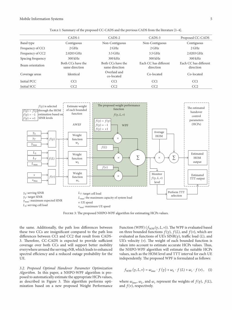
Table 1: Summary of the proposed CC-CADS and the previous CADS from the literature [1–4].

CADS-1 CADS-2 CADS-3 Proposed CC-CADSBand type Contiguous Non-Contiguous Non-Contiguous ContiguousFrequency of CC1 2GHz 2GHz 2GHz 2GHzFrequency of CC2 2.0203GHz 3.5GHz 3.5GHz 2.0203GHzSpacing frequency 300 kHz 300 kHz 300 kHz 300 kHz

Beam orientation Both CCs have thesame direction

Both CCs have thesame direction

Each CC has differentdirection

Each CC has differentdirection

Coverage areas Identical Overlaid andco-located Co-located Co-located

Initial PCC CC1 CC1 CC1 CC1Initial SCC CC2 CC2 CC2 CC2

Weight function

Estimate weight of each bounded

function

AWEF

Average HOM

Estimated HOM output

Estimated TTT output

Monitor

level

Perform TTT selection

through the HOMestimation based on SINR levels

The proposed weight performance function

WPF

Weight function

Weight function

f(L)

The estimated handovercontrol

parameters(HCPs)

∑∑

f(𝛾, L, v)

f(𝛾, L, v)

f(�)

f(�)

f(𝛾) = f(𝛾)

f(𝛾) = −1

f(𝛾) = +1

�: UE speed�max: maximum UE speedLS

LT: target cell loadLmax: the maximum capacity of system load

𝛾S: serving SINR𝛾T: target SINR𝛾max: maximum expected SINR

w�

wL

w𝛾

f(𝛾)

f(L)

f(𝛾)

f(𝛾) is selected= f(𝛾)

f(𝛾) = −1f(𝛾) = +1

𝛾S

𝛾T

𝛾max

LS

LT

Lmax

�

�

Max

×

× ×

×

: serving cell load

Figure 3: The proposed NHPO-WPF algorithm for estimating HCPs values.

the same. Additionally, the path loss differences betweenthese two CCs are insignificant compared to the path lossdifferences between CC1 and CC2 that result from CADS-3. Therefore, CC-CADS is expected to provide sufficientcoverage over both CCs and will support better mobilityeverywhere around the serving eNB,which leads to enhancedspectral efficiency and a reduced outage probability for theUE.

3.2. Proposed Optimal Handover Parameter OptimizationAlgorithm. In this paper, a NHPO-WPF algorithm is pro-posed to automatically estimate the appropriate HCPs values,as described in Figure 3. This algorithm performs opti-mization based on a new proposed Weight Performance

Function (WPF) (𝑓WPF(𝛾, 𝐿, V)). TheWPF is evaluated basedon three bounded functions 𝑓(𝛾), 𝑓(𝐿), and 𝑓(V), which areevaluated as functions of UE’s SINR(𝛾), traffic load (𝐿), andUE’s velocity (V). The weight of each bounded function istaken into account to estimate accurate HCPs values. Thus,the NHPO-WPF algorithm will estimate the suitable HCPsvalues, such as the HOM level and TTT interval for each UEindependently. The proposed WPF is formulated as follows:

𝑓WPF (𝛾, 𝐿, V) = 𝜔sinr ⋅ 𝑓 (𝛾) + 𝜔𝐿 ⋅ 𝑓 (𝐿) + 𝜔V ⋅ 𝑓 (V) , (1)

where 𝜔sinr, 𝜔𝐿, and 𝜔V represent the weights of 𝑓(𝛾), 𝑓(𝐿),and 𝑓(V), respectively.


The weight of each bounded function (𝜔sinr, 𝜔𝐿, and 𝜔V)is automatically determined by an automatic proposedweightestimator function (AWF), which is formulated as

𝜔𝑥 = 1 − 𝑓 (𝑥)∑𝐹𝑖=1 (1 − 𝑓 (𝑥𝑖)) , (2)

where 𝜔𝑥 represents the weight of function 𝑓(𝑥), which canbe 𝑓(𝛾), 𝑓(𝐿), or 𝑓(V), 𝐹 denotes the optimizing parametersfactor, which represents the total number of parameters thatare considered for optimizing HCPs (this is set to 3 becauseonly three factors are considered (𝛾, 𝐿, and V)), and 𝑓(𝑥𝑖) isa function of 𝑥𝑖, whereas 𝑥1, 𝑥2, and 𝑥3 denote 𝛾, 𝐿, and V,respectively.

𝑓(𝛾) is a function of the SINR, which is expressed by

𝑓 (𝛾) = 𝛾𝑇 − 𝛾𝑆𝛾max

, (3)

where 𝛾𝑆 and 𝛾𝑇 represent the SINRs over the serving PCCand the selected target CCs, respectively, and 𝛾max is themaximum expected SINR level measured at the UE, whichis assumed to be 30 dB.

𝑓(𝐿) is a function of the traffic loads, which is expressedby

𝑓 (𝐿) = 𝐿𝑇 − 𝐿𝑆𝐿max

, (4)

where 𝐿𝑇 and 𝐿𝑆 represent the occupant target and servingtraffic loads, respectively, and 𝐿max represents the maximumload capacity of the system.

𝑓(V) is a bounded function that is evaluated as a functionof the UE’s speed V. It is expressed by

𝑓 (V) = 2 ⋅ log2 (1 + VVmax

) − 1, (5)

where V represents the UE’s velocity and Vmax representsthe maximum expected velocity of the UE. It is assumedroughly to be 140 km for theoretical investigation. In theactual system, it can also be assumed based on the actualenvironment (i.e., urban, suburban area).

The estimated value of𝑓WPF(𝛾, 𝐿, V) is used to estimate theHOM level and to select the suitable TTT interval for eachUE independently as illustrated in Figure 3. The HOM levelis estimated bymultiplying𝑓WPF(𝛾, 𝐿, V) by the averageHOMlevel (𝑀Avg), and the result is combined with𝑀Avg, which isevaluated by

𝑀Avg = (𝑀max −𝑀min)2 , (6)

where 𝑀max and 𝑀min denote the maximum and minimumhandover margin, which are set to 10 dB and 0 dB, respec-tively.

Similar to the HOM, TTT intervals are estimated dynam-ically through the computed 𝑓WPF values. This dynamicupdate of the TTT intervals provides a more accurate deter-mination of the TTT as compared to the TTT steps defined

in the 3GPP standard. The update in TTT is denoted as Δ𝑇,which is estimated by the following model:

Δ𝑇 ={{{{{{{{{

𝑍1 if 𝑇min < 𝑇 < 𝑇max

𝑍2 if 𝑇 = 𝑇min

𝑍3 if 𝑇 = 𝑇max,(7)

where 𝑍1, 𝑍2, and 𝑍3 are represented by (8), (9), and (10),respectively:

𝑍1 = {{{𝑇 − 𝜌 if 𝑓WPF ≤ 𝑓WPF + Q

𝑇 + 𝜌 if 𝑓WPF ≥ 𝑓WPF + Q, (8)

𝑍2 = {{{𝑇 if 𝑓WPF ≤ 𝑓WPF + Q

𝑇 + 𝜌 if 𝑓WPF ≥ 𝑓WPF + Q, (9)

𝑍3 = {{{𝑇 − 𝜌 if 𝑓WPF ≤ 𝑓WPF + Q

𝑇 if 𝑓WPF ≥ 𝑓WPF + Q, (10)

where 𝜌 and Q represent the optimization interval and steplevel, respectively.

The constants, 𝜌 andQ, are meant to adjust the resolutionin which the TTT intervals are updated. If these constants areselected to be small, higher resolution of TTT is achieved.However, too high TTT resolution may impose high com-putational complexity and delays to the system. Thus, forsimplicity, the values of 𝜌 and Q are selected to be 0.04 s and0.1, respectively, throughout all the simulations. Furthermore,it can be noticed that when the update value is saturated at𝑇max or 𝑇min, then no further update is considered. 𝑇max or𝑇min is determined from the 3GPP recommendations as 0.0 sand 5.12 s, respectively.

The initial values of HOM and TTT for all the imple-mented HPO algorithms are assumed to be 2 dB and 100milliseconds, respectively.

Formore simplicity, the proposedNHPO-WPF algorithmis simplified and summarized in Table 2. Meanwhile, it iscompared with some of the most related algorithms selectedfrom the literature. In this comparison, the significant factorsthat are used to optimize handover control parameters arepresented. These factors can be briefly defined as follows.

Optimization Factors. Optimization factors are the influenceelements in the algorithm that are used to optimize handovercontrol parameters.

Optimized HCPs. They are the handover control parametersthat are considered to be optimized (estimated) automaticallybased on certain condition.

Initial HCPs Values. They are the initial handover controlparameters values that are introduced at the initial setup ofthe system.


Table 2: Comparison the proposed NHPO-WPF algorithm with the most HPO related algorithms.

Algorithm name(Authers)

HOP-Dis(Zhu and Kwak [15])

WPHPO(Balan et al. [12, 13])

HPO-FLC(Munoz et al. [14])

Proposed AlgorithmNHPO-WPF

Optimizationmethodology

Automatic adjustmentbased on distance

Automatic adjustmentbased on HPI

Automatic adjustmentbased on FLC

Dynamic adjustment basedonWPF

Optimization factors Distance(i) HFP(ii) HPPP(iii) DCP

(i) CDR(ii) HOR

(i) SINR(ii) UE’s speed(iii) Cell load

Optimized HCPs HOM (i) HOM(ii) TTT

(i) Only HOM(ii) TTT is set to a fixed

value

(i) HOM(ii) TTT

Initial HCPs values HOM = 2 dBTTT = 100ms

HOM = 8 dBTTT = 160ms



Optimization level Based on distance HOM = 0.5 dBTTT = based on 3GPP steps HOM = 1 dB (i) HOM = 2 dB

(ii) TTT not fixedOptimization updatetime — 𝜌 = 180 s 𝜌 = 0.1 s 𝜌 = 0.05 sOptimization updateprocess Performed for all eNBs Performed for all eNBs Performed for all eNBs Performed for each UE

individually

Optimization Level. It is the increment or decrement level inthe handover control parameters.

Optimization Update Time. It is the duration that is separatedbetween two optimization processes.

Optimization Update Process. It is the level of optimizationover the system; for example, the optimization is performedfor one UE, sector, eNB, or overall the system.

4. Simulation Model

4.1. System Layout Model. The LTE-Advanced system can bemodeled as shown in Figure 4 and is built based on 3GPPspecifications that were introduced in [16, 17]. The networkconsists of 61 macrohexagonal cell layout models, which arebuilt with an intersite distance of 500m for each cell. Everyhexagonal cell contains one eNB at its center, and each cellconsists of three sectors with two aggregated CCs in eachsector. Therefore, the network contains 61 cells, which areequivalent to 183 sectors. The transmission powers from theeNBs in the CCs are assumed to be the same. However, thesix eNBs that are located in the first tier are considered tobe the stations that cause interference to the UE during thesimulation time at any position 𝑥. The movement of all theUEs is considered to occur only in the first 37 hexagonalcells.Thus, when the UEmoves from the serving to the targeteNBs, it should be surrounded by six eNBs. These six eNBsare considered to be the stations that cause the interferencefor the UE.

The Frequency Reuse Factor (FRF) is assumed to be one,200 UEs are generated randomly in the serving cell, and theUEs in the target eNBs are generated and removed randomly.

−4000 −2000 0 2000 4000−4000

−3000

−2000

−1000

0

1000

2000

3000

4000

12

34

5

67

89

1011

12

1314

1516

17

18

19

2021

2223

2425

26

27

2829

3031

3233

34

35

36

37

3839

4041

4243

4445

46

47

48

4950

5152

5354

5556

57

58

59

60

61

12

34

5

67

89

1011

12

1314

1516

17

18

19

2021

2223

2425

26

27

2829

3031

3233

34

35

36

37

3839

4041

4243

4445

46

47

48

4950

5152

5354

5556

57

58

59

60

61

eNB-to-UE X location (m)

eNB-

to-U

E Y

loca

tion

(m)

UEeNB

Figure 4: LTE-Advanced systemmodelwith 61 hexagonal cells, eachof which consists of three sectors.

The random generation and removal of UEs in the targeteNBs are intended to mimic the random generation of trafficin the simulation. The UEs are generated at random uniformpositions in the cells, and each UE moves randomly at afixed speed throughout the simulation, which contains tendifferentmobile speeds.The speeds range from typical vehicle


Sector # 2Sector # 3

Sector # 1

CC1 & CC2 CC1 & CC2Beam angle = 4

CC1 & CC2Beam angle = 300∘

Beam angle = 180∘ 5∘

(a) CADS-1 and CADS-2

Sector # 2

Sector # 3

Sector # 1CC1

CC2

CC1

CC2

CC1

CC1

Beam angle = 170∘

Beam angle = 150∘

Beam angle = 220∘ Beam angle = 330∘

Beam angle = 30∘

Beam angle = 90∘

(b) CC-CADS and CADS-3

Figure 5: Beam directions of CC1 and CC2 based on different CADSs.

speeds in urban areas (40 km/hour) to a high train speed sce-nario (140 km/hour). The Adaptive Modulation and Coding(AMC) scheme is considered based on the sets of modulationschemes (MS) and Coding Rate (CR) that were introducedin [18–20]. In addition, to achieve accuracy in the highperformance evaluation, detailed models for the handoverprocedure for LTE, the RLF detection, the reestablishmentprocedure, and the Non-Access Stratum (NAS) recoveryprocedure are considered in the simulation. The essentialparameters that are used in the simulation are listed inTable 3. These parameters are taken based on LTE-Advancedsystem profile that was defined by 3GPP specifications[16–22].

4.2. Configuration of Carrier Aggregation Deployment Sce-narios. Three CA deployment scenarios are considered andcompared with CC-CADS. In CADS-1, the operating fre-quencies for CC1 and CC2 are assumed to be 2GHz and2.023GHz, respectively, and the beams of both CCs aredirected in the same directions as shown in Figure 5(a).In CADS-2, the operating frequencies for CC1 and CC2are assumed to be 2GHz and 3.5 GHz, respectively, andthe beams of both CCs are directed in the same directionsFigure 5(a). In CADS-3, the operating frequencies for CC1and CC2 are assumed to be 2GHz and 3.5GHz, respectively,and the beam of each CC is directed toward the cell boundaryof the other CC. In CC-CADS, the proposed operatingfrequencies for CC1 and CC2 are assumed to be 2GHz and2.023GHz, respectively, and the beam of each CC is directedtoward the cell boundary of the other CC. All the operatingfrequencies are assumed based on the agreed band scenariosfor the Rel. 12 timeframe [17]. However, both CCs in CC-CADS are expected to provide sufficient coverage, and bothCCs can support mobility.

In CADS-3 and CC-CADS, the beam of each CC isdirected in a different direction, and each carrier is pointedtoward a different flat side of the hexagonal cell for all three-sector sites as shown in Figure 5(b). Thus, the main beam

Table 3: Simulation parameters [16–22].

Parameter Assumption

Cellular layoutHexagonal grid, 61 hexagonalcells, 3 sectors per cell, 2 CCs

per sectorMinimum distance between UEand eNB ≥35 meters

Total eNB TX power 46 dBm per CCShadowing standard deviation 8 dBWhite noise power density (𝑁𝑡) −174 dBm/HzeNBs noise figure 5 dBThermal noise power 𝑁𝑃 = 𝑁𝑡+10 log (BW×106) dBUE noise figure 9 dB

Operation carrier bandwidth 20MHz for each, carrier PCCand SCC

Total system bandwidth 40MHz (2CCs × 20MHz)Number of PRBs/CCs 100 PRB/CCNumber subcarriers/RBs 12 subcarriers per RBNumber of OFDM symbols persubframe 7

Subcarrier spacing 15 kHzResource block bandwidth 180 kHz𝑄 rxlevmin −101.5 dBMeasurement interval 50ms for PCC and SCCTime-to-Trigger (TTT) range 0 to 5120msHO margin Selected adaptively [dB]Each𝑋2-interface delay 10msEach eNB process delay 10msT310 10 s𝑇critical 2 seconds

of CC2 is directed in a different direction than the mainbeam of CC1, and the beam of CC2 is directed toward the


(1) If Target RSRP > Serving RSRP + HOM then(2) If Trigger timer ≥ TTT then(3) Handover Decission ← True(4) else(5) Handover Decission ← false(6) Run Trigger Timer(7) end(8) else(9) Handover Decission ← false(10) Reset Trigger Timer(11) endHOM: Handover Margin Value.

Algorithm 1: Handover decision algorithm.

cell boundary of CC1. Therefore, the beams of CC1 in sectors1, 2, and 3 are aimed at beam angles of 30∘, 150∘, and 270∘,respectively, and the beams of CC2 in sectors 1, 2, and 3 areaimed at beam angles of 90∘, 210∘, and 330∘, respectively, asillustrated in Figure 5(b).

4.3. Simulation Scenario. In this paper, the RSRP is measuredperiodically during every measurement interval to evaluatethe triggering Measurement Reports (MR) as performed inthe real UE. The measurement is performed periodically forthe PCCs and SCCs simultaneously from all neighboringeNBs based on the RSRP level. The best CC from each sectoris then selected and ordered in a list based on the RSRP level.The cell that provides the best RSRP is always selected as thetarget cell candidate. After the target cell has been reported,the serving eNB will make a handover decision based onthe best target cell. The serving eNB makes the handoverdecision based on the qualities of the serving RSRPs over thePCC and the quality of the selected target RSRPs. When thetarget RSRP is greater than the serving RSRP by the handovermargin level during the TTT period, the serving eNB makesa handover decision and sends the handover request messageto the target eNB.The handover decision can be expressed byAlgorithm 1.

If the handover decision is true, the serving eNB preparesto perform the handover by sending a handover requestmessage to the target eNB, and theUEwill enter the handoverprocedure to establish a connection with the target eNB. Thehandover procedure is performed based on the handoverprocedure of the LTE-Advanced system as described in [16].Once the target eNB receives the handover request message,it will start an admission control. If the admission controldecision is true, the target eNB will send a handover requestacknowledge to the serving eNB, which in turn will begin thedownlink (DL) allocation. Once the UE receives the RRC-Connection-Reconfiguration message with the necessaryparameters, it will begin to execute the handover to the targeteNB.

ThedownlinkRSRP is evaluated andupdated periodically(whether the handover request has been sent or not) to detectthe radio link connection’s status. If a RLF is detected, the

reestablishment request is sent to the target eNB to performthe Radio Resource Control (RRC) reestablishment proce-dure; the timer T310 (the maximum time allowed to recovera connection through the RRC reestablishment procedure)will be started, and cell reselection will be performed. Next,the UE attempts to find a suitable cell that can providean RSRP greater than the minimum required receive level(Q rxlevmin) in the cell. Once the UE finds a suitable cell,it will select that cell as the target cell; if the UE findsmultiple suitable cells, the UE will select the best cell as thetarget cell. Once the target cell has been selected, the UEsends a reestablishment request message to the cell, and theRCC reestablishment procedure is performed. However, ifthe UE fails to find a suitable cell within the T310 period,the reestablishment procedure will fail, and the UE proceedsto the NAS recovery procedure. If the RRC reestablishmentattempt fails, the UE will attempt to perform the NASrecovery procedure to recover the connection. The UE willcontinue with the attempt to find a suitable cell after thetimer T310 has expired; once it finds a suitable cell, it willperform the NAS recovery procedure on it. If the NASrecovery procedure fails, the UE will restart the search fora suitable cell. Once the UE finds a suitable cell, it willattempt to perform aNAS recovery procedure on the selectedeNB again. The process of searching and performing theNAS recovery procedure will continue until the UE finds asuitable cell and successfully recovers the connection usingthe NAS recovery procedure. These recovery procedures areconsidered in the simulation to enhance the model andaccurately evaluate the performance of the handover with theCA technique as performed in the real network. Moreover,all the failure events are counted together with the U-planeinterruption time caused by these events.

4.4. Handover Scenarios. The introduction of the CA tech-nique in mobile cellular systems creates an additional han-dover scenario, which leads to an increased handover rate. InLTE systems (Rel. 8 and 9), handover occurs between eNBsin different cells or between different sectors of the samecell. However, with the advent of the CA technique in LTE-Advanced systems, additional handovers occur between com-ponent carriers in the same sector, such as from F1 to F2 orfrom F2 to F1. Five handover scenarios can occur in an LTE-Advanced system based on CA technique: (i) interfrequencyintrasector and intra-eNBhandover, (ii) intrafrequency inter-sector and intra-eNB handover, (iii) interfrequency intersec-tor and intra-eNB handover, (iv) intrafrequency inter-eNBhandover, and (v) interfrequency inter-eNB handover [23].All these handover scenarios are considered in this paper.

Intrafrequency means that the target and the serving car-rier frequencies are the same, whereas interfrequency meansthat the target and serving carrier frequencies are different.Intrasector means that the target and serving sectors arethe same and intersector means that the target and servingsectors are different. Intra-eNB means that the target andserving eNBs are the same, and inter-eNB means that thetarget and serving eNBs are different. All these handoverscenarios are illustrated in Figure 6.


PCC = CC2Active CC1 & CC2

Sector 2

PCC = CC1

Active

CC1 & CC2

Sector 2


Sector 1

PCC = CC1

Active CC1 &

CC2Sector 1

eNB1

Scenario 2

Scenario 1

Scenario 3

CC CC

(a) Intra-eNB handover


Sector 1

PCC = CC1

Active CC1 & CC2

Sector 1

eNB1


Sector 2

PCC = CC1

Active

CC1 & CC2

Sector 2

eNB2

Scenario 4

C2

(b) Intrafrequency inter-eNB handover


Sector 1

PCC = CC1

Active CC1 & CC2

Sector 1

eNB1


Sector 2

PCC = CC2

Active

CC1 & CC2

Sector 2

eNB2

Scenario 5

C2

(c) Interfrequency inter-eNB handover

Figure 6: Frequency handover scenarios.


5. Evaluation of Handover Performance

5.1. Downlink SINR Evaluation. This paper applies a macro-cell propagation model that considers the path loss, shadow-ing, and Rayleigh fast fading effects. The propagation modelcan be formulated as [17]:

PL = 58.8 + 37.6 log10 (𝑑) + 21 log10 (𝑓𝑐) + 𝜓dB + 𝜗dB, (11)

where 𝑑 represents the distance between the UE and the eNBin kilometers, 𝑓𝑐 is the operating carrier frequency in MHz,𝜓dB is a log-normal shadowing in dB, and 𝜗dB represents theRayleigh fast fading effect in dB.

The transmitted signals in the DL transmission in anLTE-Advanced network based on the CA technique and anOrthogonal Frequency-Division Multiple Access (OFDMA)scheme are considered, where every eNB can serve each UEby 𝑁UE

sc subcarriers over 𝑁UECC CCs assigned to each UE.

This scenario means that each UE has the ability to receivedata from multiple subcarriers (𝑁UE

sc ) over several CCs. Thedefinition of the Physical Resource Block (PRB), which wasintroduced in [18–20], is considered in this paper. However,if the total number of subcarriers in a single CC is representedby𝑁CC

sc , the total transmission power 𝑃TX of the eNB on eachCC is distributed equally over all the subcarriers. Thus, thetotal transmission power of each subcarrier is expressed by[24]

𝑃TX(𝑚,𝑘) = 𝑃TX𝑁CC

sc. (12)

The transmitted power, 𝑃TX(𝑚,𝑘) , over any subcarrier fromany eNB in an LTE-Advanced system is assumed to be thesame over any CC. Therefore, the useful received signalpower 𝑃RX(𝑚,𝑘) at UE on subcarrier k over CC𝑚 in the DLtransmission can be expressed by

𝑃RX(𝑚,𝑘) = 𝑃TX(𝑚,𝑘) + 𝐺TX𝑚 + 𝐺RX − PL𝑚 (dB) , (13)

where𝑃TX(𝑚,𝑘) represents the transmitted signal power on sub-carrier 𝑘 over CC𝑚 in dBm, 𝐺TX𝑚 represents the transmitterantenna gain over CC𝑚 in dB, 𝐺RX represents the receiverantenna gain in dB, and PL𝑚 represents the path loss betweenUE and eNB over CC𝑚 in dB.

Only the interference signals received by the UE from thesix neighboring eNBs located in the first tier that surroundsthe served eNB are considered. The interference signals thatare received from the eNBs located in the second tier will beneglected due to the weakness of these interference signalscompared with those from the eNBs in the first tier.Thus, theinterference signals received by the UE on subcarrier 𝑘 overCC𝑚 from𝐻 neighboring eNBs located in the first tier of theserved eNB are expressed as

𝐼𝑚,𝑘 =𝐻

∑ℎ=1

𝑃int(𝑘,𝑚 ℎ) , (14)

where 𝑃int(𝑘,𝑚 ℎ) represents the interference received signalpower by the UE on subcarrier 𝑘 over CC𝑚 from theneighboring eNB ℎ.

Consequently, the SINR at the UE on subcarrier 𝑘 overCC𝑚 is expressed by

SINR𝑚,𝑘 =𝑃RX(𝑚,𝑘)

∑𝐻ℎ=1 𝑃int(𝑘,𝑚 ℎ) + 𝑃no𝑚,𝑘, (15)

where 𝑃no𝑚,𝑘 represents the noise power for the UE onsubcarrier 𝑘 over CC𝑚.5.2. UE Bit Rate. Based on the 3GPP specifications intro-duced in [18, 25, 26], one radio frame consists of tensubframes (i.e., one radio frame = 10ms), each subframeconsists of two time slots, one time slot consists of 0.5ms(i.e., 1 subframe = 1ms), and one time slot consists of 7modulation symbols if a normal Cyclic Prefix (CP) lengthis used, in which the number of OFDMA symbols in eachslot depends on the CP length and the configured subcarrierspacing. Each modulation symbol consists of 2, 4, or 6 bits ifQPSK, 16-QAM, or 64-QAM is used as modulation scheme,respectively.

As explained in detail in [18, 26], the transmitted signalin each time slot is configured by one or several resourcegrids (RG), eachRG consists of several PRBs (𝑁DL

RB ), each PRBconsists of𝑁RB

sc subcarriers, and each subcarrier is configuredby 𝑁DL

symb OFDMA symbols. The quantity of DL PRBs 𝑁DLRB

depends on the entireDL transmission bandwidth configuredin the cell. Thus, a PRB consists of 𝑁DL

symb × 𝑁RBsc resource

elements that correspond to one slot in the time domain and180 kHz in the frequency domain. Each modulation symbolcarries 𝑚symb

bit bits, which depend on the modulation schemethat is selected. Consequently, the total number of bits in onetime slot that consists of 𝑁sc

symb modulation symbols can beexpressed by

𝐵scbit = 𝑁sc

symb𝑚symbbit . (16)

Each PRB consists of 𝑁RBsc subcarriers. Therefore, the total

number of bits in one PRB (𝐵RBbit ) can be given by

𝐵RBbit = 𝑁RB

sc 𝑁scsymb𝑚symb

bit . (17)

However, each PRB contains 𝑁RBRS resource elements that

are configured as reference symbols, which correspond to𝑁RB

RS OFDM symbols in the time domain [26]. These, 𝑁RBRS ,

reference symbols allow the UE to estimate the channelcondition. Therefore, the number of useful bits in one PRBcan be given by

𝐵RBbit = 𝑁RB

sc (𝑁scsymb − 𝑁RB

RS )𝑚symbbit . (18)

The total number of PRBs that can be assigned to each activeUE (𝑁UE

RB ) depends on the number of active UEs in the celland the total available system bandwidth. The numbers ofPRBs that can be assigned to eachUE (𝑁UE

RB ) can be expressedby

𝑁UERB = 𝑁Total DL

RB𝑁sys

UEs, (19)


where 𝑁Total DLRB represents the total number of available DL

PRBs over the entire system bandwidth and𝑁sysUEs represents

the total number of active UEs in the system. Consequently,the total number of useful bits that can be transmitted to eachUE 𝐵UE

bit can be expressed by

𝐵UEbit = 𝑁UE

RB𝑁RBsc 𝑁sc

symb𝑚symbbit . (20)

The transmitted bits from the served eNB to the end UEinclude the code rate bits; therefore, the effect of the coderate, 𝐸, is considered in the evaluation.The total received UEthroughput that can be correctly received from multiple CCsover the entire system bandwidth can be formulated by

𝑅UEbit =

𝑁UERB𝑁RB

sc (Nscsymb − 𝑁RB

RS )𝑚symbbit

𝑇𝑗 𝐸, (21)

where 𝑇𝑗 is the time over which the data bits are received forUE𝑗.

5.3. Downlink Spectral Efficiency. The spectral efficiency canbe represented mathematically by aggregating the total UE’sthroughput that is correctly received by the UE at a specifictime and dividing by the total UE channel bandwidth.Therefore, the normalized spectral efficiency 𝜂𝑗 for UE𝑗 canbe expressed by [25]

𝜂𝑗 = 𝑅UEbit

𝑇𝑗𝜔UEBW

(bits/sec/Hz) , (22)

where 𝑅UEbit denotes the number of correctly received bits for

UE𝑗 in a system and 𝜔UEBW represents the UE’s channel band-

width, which can be calculated by multiplying the number ofPRBs assigned to UE𝑗, 𝑁UE

RB , by the PRB’s bandwidth (𝐵RB)and can be expressed by

𝜔UEBW = 𝑁UE

RB𝐵RB. (23)

Consequently, from (21) and (22), the UE’s spectral efficiencybased on a single component carrier can be expressed by

𝜂𝑗 =𝑁UE

RB𝑁RBsc (𝑁sc

symb − 𝑁RBRS )𝑚symb

bit

𝑇𝑗𝜔UEBW

𝐸 (bps/Hz) . (24)

Because this study considers the CA technique based on 𝑈component carries, the total UE’s spectral efficiency can beformulated based on (21) as

𝜂𝑗 =𝑈

∑𝑚=1

𝑁UERB (CC𝑚)𝑁RB

sc (𝑁scsymb − 𝑁RB

RS )𝑚symbbit

𝑇𝑗𝜔UEBW

𝐸 (bps/Hz) . (25)

5.4. Cell Edge UE’s Spectral Efficiency. The cell edge spectralefficiency is an important measurement performance metricthat is used to evaluate the throughput at the cell boundaryin UE mobility studies of cellular communication systems.Because the proposed CA deployment scenario and CADS-3 are scenarios that can contribute to enhancing the cell

edge throughput, the cell edge UE’s spectral efficiency will beevaluated to identify the enhancements that can be achievedin each scenario. The cell edge throughput will be evaluatedto assess the enhancement that can be achieved at thecell boundary using the proposed CC-CADS compared tostandard CADSs.The cell edge UE’s spectral efficiency can bedefined as the 5th percentile of the Cumulative DistributionFunction (CDF) of the normalized UE’s spectral efficiency[23], which is defined as the average UE throughput overan appointed period divided by the channel bandwidth asmeasured in bit/s/Hz. Therefore, the cell edge UE’s spectralefficiency is a measure of the perceived “quality of service”for the 5% of UEs with the lowest UE throughput.

5.5. Handover Probability. The handover probability (HOP)is the likelihood of switching the radio link connection forthe served UE from the source to the target cells duringactive mode operation [27]. In other words, HOP is theprobability of handing over the served UE from the servingto the target cells once the serving signal quality is becomingworse than the target signal strength by a HOM level. HOPis a significant performance indicator that is used to measuresystem performance and can be represented by

𝑃HO = 𝑃𝑟 [𝛽𝑇 − 𝛽𝑆 ≥ 𝑀] , (26)

where 𝛽𝑇 and 𝛽𝑆 represent the signal levels of the target andserving cells, respectively, and 𝑀 represents the HOM level.The handover probability can be translated into the averagenumber of handovers per call over all the served UEs toincrease the performance evaluation accuracy. The averagehandover probability rate is calculated in every simulationcycle over all the served UEs in the system.Thus, the averagenumber of handovers per UE (𝑃HO) can be expressed by

𝑃HO = ∑𝑁sysUEs𝑗=1 𝑃HO (𝑗)𝑁sys

UEs, (27)

where 𝑁sysUEs represents the total number of served UEs over

the system and 𝑃HO(𝑗) represents the handover probabilityfor UE𝑗.

5.6. Handover Ping-Pong Probability. HPPP is an importantmetric in studies of handover; it is used to measure the num-ber of unnecessary handovers that are performed betweentwo adjacent cells [27].The handover will encounter the ping-pong effect if UE-i leaves the serving eNB-A to the targeteNB-B and is then handed back to the serving eNB-A in aperiod less than the critical interval𝑇critical (the time requiredto measure the unnecessary handover between adjacent cells;it is assumed to be 2 seconds). When the handover takesplace, the HPPP can be measured based on the followingprobability:

𝑃HPPP = 𝑃 [𝑇Interval ≤ 𝑇critical] , (28)

where 𝑇Interval represents the time interval between the UEleaving the serving eNB-A and being returned to the sameeNB-A. Thus, 𝑇Interval can be expressed by

𝑇Interval = 𝑇Leave − 𝑇handed back, (29)


where 𝑇Leave represents the time the UE leaves the servingeNB-A and 𝑇handed back represents the time the UE is handedback to the serving eNB-A. If the UE is handed backto the old serving eNB (eNB-A) and 𝑇Interval is less than𝑇critical (𝑇Interval < 𝑇critical), the handover is recorded as aping-pong handover. The number of ping-pong handoversis recorded for each UE, and the average HPPP over allthe served UEs is recorded in every simulation cycle 𝑡 toincrease the accuracy of the performance evaluation. Theaverage HPPP (𝐴HPPP) per UE during simulation cycle 𝑡 canbe represented by

𝐴HPPP = 𝑁sysHPP

𝑁sysRHP

, (30)

where 𝑁sysHPP represents the total number of handover ping-

pongs over all the system and 𝑁sysRHP is the total number of

requested handovers, which is given by

𝑁sysRHP = 𝑁sys

SHP + 𝑁sysFHP, (31)

where 𝑁sysSHP and 𝑁sys

No-HPP are the numbers of successful andfailed handovers.The number of successful handovers (𝑁sys

SHP)includes the ping-pong (𝑁sys

HPP) andnon-ping-pong (𝑁sysNo-HPP)

handover numbers and is given by

𝑁sysSHP = 𝑁sys

HPP + 𝑁sysNo-HPP. (32)

5.7. Handover Failure Ratio. Handover failure normallyoccurs after the handover request has been sent to the targeteNB [25]. Two cases can cause a handover failure: (i) lack oftarget resource availability and (ii) loss of coverage. In theformer case, the handover failure occurs after the handoverrequest is sent to the target eNB and the handover procedureis initiated but insufficient resources are available for thetarget eNB to complete the handover procedure. In the lattercase, the handover failure occurs if the UE moves out of thecoverage of the target eNB before the handover procedureis finalized. The total handover failure ratio (𝑁Totl

FHP) can beexpressed as

𝑁TotlFHP = 𝑁sys

FHP

𝑁sysFHP + 𝑁sys

SHP. (33)

5.8. Outage Probability. The outage probability (𝑃out) of thecell can be defined as the percentage of area within the cellthat does not meet its minimum power requirement 𝑃min,which can be defined as the probability that the instanta-neously received SINR(𝛾) falls below a given threshold level,where the threshold level 𝛾Thr represents the minimum SINRlevel below which the performance becomes unacceptable.The outage probability for cellular mobile communicationsystems is represented mathematically as the probabilitythat the instantaneously received SINR(𝛾) falls below thethreshold level 𝛾Thr [28, 29] and is normally represented as

𝑃out = 𝑃 [𝛾 < 𝛾Thr] = 1 − 𝑃 [𝛾 > 𝛾Thr] . (34)

In this simulation, the outage probability is recorded whenthe serving SINR of UE𝑗 during simulation cycle 𝑡 falls below

2.2 2.4 2.6 2.8 3 3.2 3.4 3.6 3.8 4 4.20

0.1

0.2

0.3

0.4

0.5

0.6

0.7

0.8

0.9

1

Average UE’s spectral efficiency (bps/Hz)

Empirical CDF

CADS-1CADS-2

CADS-3CC-CADS

CDF

of sp

ectr

al effi

cien

cy p

roba

bilit

y

Figure 7: Average UE’s spectral efficiencies with different CADSs.

a given threshold level, and the average outage probability forall UEs is evaluated during every simulation cycle to increasethe accuracy of the results. From (34), the average outageprobability can be simplified as

𝑃out =∑𝑁𝑗=1 1 − 𝑃 [𝛾𝑗 > 𝛾Thr]

𝑁sysUEs

. (35)

6. Results and Discussions

In this section, the performance results of both proposedsolutions will be presented and discussed. First, the achiev-able system performance results of CC-CADS will be pre-sented and compared with those of three different CADSs.Then, the system performance results from the NHPO-WPF algorithm based on CC-CADS will be presented andcompared with the conventional HPO, WPHPO, and FLCalgorithms.

6.1. Carrier Aggregation Deployment Scenario with SufficientCoverage. This subsection presents the system performanceresults of CC-CADS and compares them with the results ofthree standard CADSs: CADS-1, CADS-2, and CADS-3. Allthe results presented in this subsection were simulated basedon a conventional HPO algorithm with ten different mobilespeeds.The results are presented in terms of the UE’s spectralefficiency, the cell edgeUE’s spectral efficiency, and the outageprobability. The main goal of CC-CADS is to enhance thespectral efficiency and reduce the outage probability.

Figures 7 and 8 show the average UE’s spectral effi-ciencies and the average cell edge UE’s spectral efficiencies,respectively. These results represent the average values overall UEs and all mobile speeds for four different CADSs.The results show that the CADS-1 and CADS-2 scenariosgive the same spectral efficiency. These identical results are


1 1.5 2 2.5 3 3.52.2

2.4

2.6

2.8

3

3.2

3.4

3.6

3.8

Average UE’s SINR over PCC (dB)

Aver

age U

E’s c

ell e

dge s

pect

ral e

ffici

ency

CADS-1CADS-2

CADS-3CC-CADS

over

PCC

(bps

/Hz)

Figure 8: Average cell edge UE’s spectral efficiency versus SINR fordifferent CADSs.

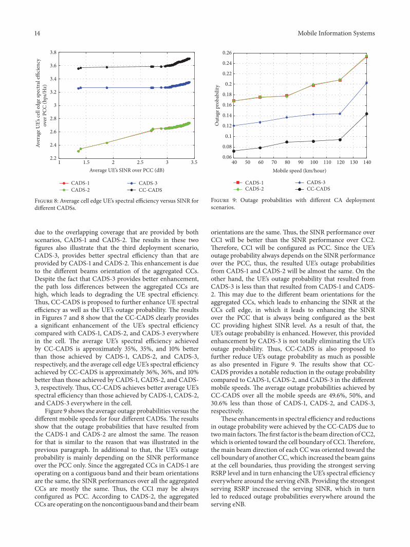
due to the overlapping coverage that are provided by bothscenarios, CADS-1 and CADS-2. The results in these twofigures also illustrate that the third deployment scenario,CADS-3, provides better spectral efficiency than that areprovided by CADS-1 and CADS-2. This enhancement is dueto the different beams orientation of the aggregated CCs.Despite the fact that CADS-3 provides better enhancement,the path loss differences between the aggregated CCs arehigh, which leads to degrading the UE spectral efficiency.Thus, CC-CADS is proposed to further enhance UE spectralefficiency as well as the UE’s outage probability. The resultsin Figures 7 and 8 show that the CC-CADS clearly providesa significant enhancement of the UE’s spectral efficiencycompared with CADS-1, CADS-2, and CADS-3 everywherein the cell. The average UE’s spectral efficiency achievedby CC-CADS is approximately 35%, 35%, and 10% betterthan those achieved by CADS-1, CADS-2, and CADS-3,respectively, and the average cell edge UE’s spectral efficiencyachieved by CC-CADS is approximately 36%, 36%, and 10%better than those achieved by CADS-1, CADS-2, and CADS-3, respectively. Thus, CC-CADS achieves better average UE’sspectral efficiency than those achieved by CADS-1, CADS-2,and CADS-3 everywhere in the cell.

Figure 9 shows the average outage probabilities versus thedifferent mobile speeds for four different CADSs. The resultsshow that the outage probabilities that have resulted fromthe CADS-1 and CADS-2 are almost the same. The reasonfor that is similar to the reason that was illustrated in theprevious paragraph. In additional to that, the UE’s outageprobability is mainly depending on the SINR performanceover the PCC only. Since the aggregated CCs in CADS-1 areoperating on a contiguous band and their beam orientationsare the same, the SINR performances over all the aggregatedCCs are mostly the same. Thus, the CC1 may be alwaysconfigured as PCC. According to CADS-2, the aggregatedCCs are operating on the noncontiguous band and their beam

40 50 60 70 80 90 100 110 120 130 1400.06

0.08

0.1

0.12

0.14

0.16

0.18

0.2

0.22

0.24

0.26

Mobile speed (km/hour)

Out

age p

roba

bilit

y

CADS-1CADS-2

CADS-3CC-CADS

Figure 9: Outage probabilities with different CA deploymentscenarios.

orientations are the same. Thus, the SINR performance overCC1 will be better than the SINR performance over CC2.Therefore, CC1 will be configured as PCC. Since the UE’soutage probability always depends on the SINR performanceover the PCC, thus, the resulted UE’s outage probabilitiesfrom CADS-1 and CADS-2 will be almost the same. On theother hand, the UE’s outage probability that resulted fromCADS-3 is less than that resulted from CADS-1 and CADS-2. This may due to the different beam orientations for theaggregated CCs, which leads to enhancing the SINR at theCCs cell edge, in which it leads to enhancing the SINRover the PCC that is always being configured as the bestCC providing highest SINR level. As a result of that, theUE’s outage probability is enhanced. However, this providedenhancement by CADS-3 is not totally eliminating the UE’soutage probability. Thus, CC-CADS is also proposed tofurther reduce UE’s outage probability as much as possibleas also presented in Figure 9. The results show that CC-CADS provides a notable reduction in the outage probabilitycompared to CADS-1, CADS-2, and CADS-3 in the differentmobile speeds. The average outage probabilities achieved byCC-CADS over all the mobile speeds are 49.6%, 50%, and30.6% less than those of CADS-1, CADS-2, and CADS-3,respectively.

These enhancements in spectral efficiency and reductionsin outage probability were achieved by the CC-CADS due totwomain factors.Thefirst factor is the beamdirection ofCC2,which is oriented toward the cell boundary of CC1.Therefore,the main beam direction of each CC was oriented toward thecell boundary of another CC, which increased the beam gainsat the cell boundaries, thus providing the strongest servingRSRP level and in turn enhancing the UE’s spectral efficiencyeverywhere around the serving eNB. Providing the strongestserving RSRP increased the serving SINR, which in turnled to reduced outage probabilities everywhere around theserving eNB.


The second contributing factor is the operating frequen-cies for CC1 and CC2, which are assumed to operate in acontiguous band. The coverage areas provided by these twoCCs are almost the same but have different beam directions.Thus, the path loss differences between these two CCs cannotbe compared with those based on CADS-2 or CADS-3; thepath loss that results from CC2 based on CADS-3 will behigher than that from CC2 based on CC-CADS. CC-CADSprovides a sufficient coverage area that is better than thoseprovided by CADS-1, CADS-2, and CADS-3 everywherearound the serving eNB, which leads to enhanced servingRSRP everywhere around the serving eNB.The enhancementof the serving RSRP led to an increase in the serving SINR tothe UE, which in turn increased the UE’s spectral efficiencyand reduced the UE’s outage probability.Thus, the CC-CADSprovides better UE’s spectral efficiency enhancement andoutage probability reduction everywhere around the servingeNB than CADS-1, CADS-2, and CADS-3, as illustrated inFigures 7, 8, and 9, respectively.

6.2. Optimal Handover Parameter Optimization. In this sub-section, the proposed NHPO-WPF, conventional HPO, FLC,andWPHPO algorithms are analyzed to investigate and vali-date their performance in the CA technique and to highlightthe enhancements that are achieved by the proposed NHPO-WPF algorithm as compared to the other algorithms. Firstly,an example of how the NHPO-WPF algorithm adapts theHCPs depending on the SINR, system load, and user speedis given. Then, the simulation results of these four HPOalgorithms are presented and discussed based on CC-CADS.The results show the impact of different mobile speeds on thehandover performance of proposed algorithm and the otherthree HPO algorithms. Because the proposed NHPO-WPFalgorithm is intended to enhance handover performance, thesimulation results are presented and discussed in terms ofthe average HOP, HPPP, and HFP. The average values arecalculated over all active UEs and then over all the simulationtime.

The handover control parameters estimated by the pro-posed NHPO-WPF algorithm during the simulation time areshown in Figure 10 based on the UE speeds of 120 km/houronly. The HOM and TTT are initialized at 2 dB and 100milliseconds, respectively. The aim of this simulation is tohighlight the comparative HOM and TTT values producedby the proposed algorithm at different UE speeds in contrastto the conventional and some of the literature algorithms.TheHOM and TTT are computed as averages over all the UEsin this simulation. The results are presented for three-secondtime interval. It is clear that the conventional HPO algorithmshows decay in the HOM and the TTT at all UE speeds.This can be explained by noticing that HPO algorithms aimto reduce the RLF in the network; hence it tends to reducethe HCPs. On the other hand, the FLC algorithm providedhigher HOM values as compared to the conventional HPO.However, the TTT profile produced by the FLC algorithmis in close matching to the conventional HPO. Similar tothe conventional HPO algorithm, the UE speed influence onthe HCPs values estimated by FLC algorithm is very minor.

0 0.5 1 1.5 2 2.5 3−5

0

5

10

Aver

age H

OM

leve

l (dB

)

Time (second)

0 0.5 1 1.5 2 2.5 30

100

200

300

Aver

age T

TT in

terv

al

Time (second)

HPO-CnvFLC

WPHPONHPO-WPF

(mill

iseco

nd)

Figure 10: Average HCPs values versus time with UE speed of120 km/hour.

The WPHPO algorithm estimates the HCPs parameters inthe smaller range as compared to both HOP and FLC. Thissmall estimation range may cause insufficient estimationof the HCPs values, particularly at high UE speeds. Moreimportantly, the effect of UE speed on the performance of theWPHPO is also very minor.

As the proposedNHPO-WPF algorithmconsiders theUEperformance metric as parameters to estimate the HCPs, itprovided wider HCPs estimation range. This would provideappropriate HOM and TTT levels estimation at different UEspeeds. This appropriate estimation may improve handoverperformance in general. Moreover, the effect of UE speedsinfluenced the estimation range of the proposed algorithm.This can be deduced by the comparison in Figure 10. Thisinfluence of the UE speeds is due to the considerationof UE speeds as estimation parameter in the NHPO-WPFalgorithm.

Figure 11 shows the average handover probability versusmobile speed for the NHPO-WPF, conventional HPO, FLC,andWPHPO algorithms.The results show that the proposedNHPO-WPF algorithm provides a significant reduction ofthe average handover probability compared to the conven-tional HPO, FLC, and WPHPO algorithms for all the mobilespeeds. The average HOPs that are achieved by the NHPO-WPF algorithm are approximately 95, 98, and 90% lowerthan those with the conventional HPO, FLC, and WPHPOalgorithms, respectively. Because a high HOP leads to highHPPP and HFP, the reduction of HOP will lead to significantreductions in the HPPP and HFP, which will be discussedbelow.

Figures 12 and 13 show the average HPPPs for the NHPO-WPF, conventional HPO, FLC, and WPHPO algorithmsbased on the different mobile speeds. HPPP may occur whena nonoptimal HPO algorithm is used to optimize the HCPs,which leads to estimating suboptimal HCPs values, in turn


40 50 60 70 80 90 100 110 120 130 1400

0.01

0.02

0.03

0.04

0.05

0.06

0.07

Mobile speed (km/hour)

Han

dove

r pro

babi

lity

HPO-CnvFLC

WPHPONHPO-WPF

Figure 11: Average handover probability versus mobile speed withdifferent handover parameter optimization algorithms.

0 0.5 1 1.5 2 2.5 3 3.5 4 4.5 50

0.05

0.1

0 0.5 1 1.5 2 2.5 3 3.5 4 4.5 50

0.05

0.1

Han

dove

r

prob

abili

typi

ng-p

ong

Han

dove

r

prob

abili

typi

ng-p

ong

Han

dove

r

prob

abili

typi

ng-p

ong

0 0.5 1 1.5 2 2.5 3 3.5 4 4.5 50

0.05

0.1

Time (second)

Time (second)

Time (second)

HPO-CnvFLC

WPHPONHPO-WPF

Mobile speed (140km/hour)



Figure 12: Handover ping-pong probability with different mobilespeeds based on different HPO algorithms.

leading to an increase in the number of unnecessary han-dovers (HPPP effect), especially in highmobility speeds.Thishigh HPPP effect increases the waste of network resources.The results shown in Figure 12 represent the average HPPPper UE based on the various mobile speeds (medium andhigh speeds), while the results shown in Figure 13 showthe average HPPP over the entire simulation time for eachmobile speed scenario independently. The results show thatthe proposed NHPO-WPF algorithm provides a lower HPPPthan the conventional HPO, FLC, and WPHPO algorithmsfor all the considered mobile speeds scenarios; it achieves

0 1 2 3 4 5 6 7 8 9 10Time (millisecond)

Aver

age h

ando

ver p

ing-

pong

pro

babi

lity

HPO-CnvFLC

WPHPONHPO-WPF

10−4

10−3

10−2

10−1

Figure 13: Average handover ping-pong probability over all mobilespeeds versus time, based on the HPO algorithms.

HPO-Cnv FLC WPHPO NHPO-WPF0

0.5

1

1.5

2

2.5

3

3.5

Handover parameters optimization algorithms

Han

dove

r fai

lure

pro

babi

lity

×10−3

40kmph60kmph80kmph

100 kmph120 kmph140kmph

Figure 14: Average handover failure probabilities for differentmobile speeds based on different mobility handover optimizationalgorithms.

average reductions of approximately 99.4, 99.8, and 98.6%compared to the conventional HPO, FLC, and WPHPOalgorithms, respectively.

Figure 14 shows the average HFPs from the NHPO-WPF,conventional HPO, FLC, and WPHPO algorithms for thedifferent mobile speeds. The average HFPs were calculatedover all the UEs in the system and over all simulation timesfor each mobile speed scenario independently. The results


show that the proposed NHPO-WPF algorithm achieves aconsiderable reduction of HFP compared to the conventionalHPO, FLC, and WPHPO algorithms. The average HFPsachieved by NHPO-WPF are approximately 96, 98, and92% less than those with the conventional HPO, FLC, andWPHPO algorithms, respectively. An interesting observationis that the results show greater reductions than the reductionsof the handover and handover ping-pong probabilities; this isdue to the consideration of traffic loads in the optimizationprocess, which leads to estimates of suitable HCPs. Thisindicates that the resource availability of the target cell istaken into account during the optimization process, whichin turn leads to making an accurate handover decision andperforming a successful handover as long as the resourcesare available in the target cell. It will also prevent the servingeNB from making a true handover decision if the targetcell does not have sufficient resources; this leads to moresuccessful handovers and decreases the handover failureprobability.

The results illustrate that the proposed NHPO-WPFalgorithmprovides better performance than the conventionalHPO, FLC, and WPHPO algorithms. It achieves averagereductions of all the handover performance metrics (HOP,HPPP, and HFP) of approximately 96.8, 98.8, and 93.5%compared to the conventional HPO, FLC, and WPHPOalgorithms, respectively. These reductions are mostly due tothe effect of the UE’s SINR level, velocity, and TL duringthe estimation of the HCPs; considering these parameterscontributed to estimating the appropriate HOM and TTTvalues, which led tomaking correct handover decisions.Thus,the proposedNHPO-WPF algorithmbased on theCC-CADSscenario achieves significant reductions in HOP, HPPP, andHFP compared to the conventional HPO, FLC, andWPHPOalgorithms.

7. Concluding Remarks

In this paper, two proposed solutions, known as the CC-CADS and the NHPO-WPF algorithm, were introduced andvalidated. Both solutions enhanced the system performancewhen they were applied to CA technique in the LTE-Advanced environment. The simulation results showed thatCC-CADS provided wider coverage and achieved significantenhancements compared to the standard CADSs, especiallyat the cell edge. CC-CADS achieved average UE’s spectralefficiency improvements of 35%, 35%, and 10% over thoseof CADS-1, CADS-3, and CADS-3, respectively, and reducedoutage probabilities by approximately 49.6%, 50%, and 30.6%compared to CADS-1, CADS-3, and CADS-3, respectively.The proposed NHPO-WPF algorithm provided significantenhancements compared to the conventional HPO algorithmand other algorithms from the literature. The NHPO-WPFalgorithm provided average reductions in HOP, HPPP, andHFP of approximately 96.8%, 98.8%, and 93.5% comparedto the conventional HPO, FLC, and WPHPO algorithms,respectively. Thus, the two proposed solutions providedbetter performance than the other considered scenarios andalgorithms.

Nomenclature

List of Terminologies Used in the Paper

3GPP: Third-Generation Partnership ProjectAMC: Adaptive Modulation and CodingAWF: Automatic proposed weight estimator

functionCA: Carrier aggregationCADSs: Carrier Aggregation Deployment

ScenariosCC-CADS: Coordinated Contiguous-Carrier

Aggregation Deployment ScenariosCCs: Component carriersCDF: Cumulative Distribution FunctionCDR: Call Drop RateCP: Cyclic PrefixCR: Coding RateDCP: Drop Call ProbabilityDL: DownlinkeNB: Evolved Node BFLC: Fuzzy Logic ControllerFRF: Frequency Reuse FactorHCPs: Handover Control ParametersHFP: Handover failure probabilityHOM: Handover marginHOR: Handover RatioHPI: Handover Performance IndicatorHPO: Handover Parameters OptimizationHPPP: Handover ping-pong probabilityLTE-Advanced: Long Term Evolution AdvancedMR: Measurement ReportsMS: Modulation schemesNAS: Non-Access StratumNHPO-WPF: Novel Handover Parameters Optimization

algorithm that is based on the WeightPerformance Function

OFDMA: Orthogonal Frequency-Division MultipleAccess

PRB: Physical Resource BlockRG: Resource gridsRLF: Radio Link FailureRRC: Radio Resource ControlSINR: Signal-to-Interference Noise RatioSO: Self-OptimizationTTI: Transmission Time IntervalTTT: Time-To-TriggerUE: User EquipmentWPF: Weight Performance FunctionWPHPO: Weighted Performance based on

Handover Parameter Optimization.

List of Notations Used in the Paper

𝑁DLRB : Total number of DL PRBs over one

resource grid𝑃HO: Average number of handovers per UE𝐴HPPP: Average handover ping-pong probability

per UE


𝐵RB: PRB’s bandwidth𝐵RBbit : Total number of bits over each PRB

𝐵scbit: Total number of bits over each subcarrier

𝐵UEbit : Total number of useful bits transmitted to

UE𝐺TX𝑚 : Transmitter antenna gain over CC𝑚 [dB]𝐺RX: Receiver antenna gain [dB]𝐼𝑚,𝑘: Total interferences received signals power

on subcarrier 𝑘 over CC𝑚 from all neigh-boring eNBs

𝐿𝑆: The occupant serving traffic load𝐿𝑇: The occupant target traffic load𝐿max: Maximum load capacity of the system𝑀Avg: Average handover margin level𝑀max: Maximum handover margin𝑀min: Minimum handover margin𝑁UE

CC : Total number of CCs paired to one UE𝑁Totl

FHP: Total number of handover failure ratios𝑁sys

HPP: Total number of handover ping-pongsoverall the system

𝑁sysNo-HPP: Total number of non-ping-pongs

𝑁Total DLRB : Total number of availableDLPRBs over the

entire system bandwidth𝑁UE

RB : Total number of PRBs paired to one UE𝑁sys

RHP: Total number of requested handovers𝑁RB

RS : Total number of resource elements that areconfigured as reference symbols

𝑁sysSHP: Total number of successful handovers

𝑁sysUEs: Total number of active UEs in the system

𝑁CCsc : Total number of subcarriers per CC

𝑁RBsc : Total number of DL subcarriers over one

PRB𝑁UE

sc : Total number of subcarriers paired to oneUE

𝑁DLsymb: Total number of DL symbols over one

resource grid𝑁sc

symb: Total number of modulation symbols overone subcarrier

𝑃RX(𝑚,𝑘) : UE’s received signal power on subcarrier 𝑘over CC𝑚 [dBm]

𝑃TX(𝑚,𝑘) : Transmitted signal power on subcarrier 𝑘over CC𝑚 [dBm]

𝑃int(𝑘,𝑚 ℎ) : Interference received signal power by theUE on subcarrier 𝑘 over CC𝑚 from theneighboring eNB ℎ

𝑃HO: Handover probability𝑃HO(𝑗): Handover probability for UE𝑗𝑃HPPP: Handover ping-pong probabilityPL𝑚: Path loss over CC𝑚 [dB]𝑃no𝑚,𝑘 : The noise power for the UE on subcarrier 𝑘

over CC𝑚𝑃TX: Total transmission power from the eNBover each CC

𝑅UEbit : Total number of bits received at UE within

a period of 𝑇

SINR𝑚,𝑘: SINR at the UE on subcarrier 𝑘 over CC𝑚𝑇Handed back: Time taken for the UE to be handed backto the serving eNB

𝑇Interval: The time interval between the UE leavingthe serving eNB and being returned to thesame eNB

𝑇Leave: Time taken for the UE to leave the servingeNB-A

𝑇critical: Critical interval𝑇𝑗: The data bits received time for the UE𝑗𝑇max: Maximum TTT interval𝑇min: Minimum TTT interval𝑓WPF(𝛾, 𝐿, V): Weight Performance Function𝑓𝑐: Carrier frequency𝑚symb

bit : Total number of bits over one modulationsymbol

𝑃TX(𝑚,𝑘) : Total transmission power over each subcar-rier in watt

Vmax: Maximum expected UE’s velocity𝑥1: 𝛾𝑥2: 𝐿𝑥3: V𝛽𝑆: Serving signal level𝛽𝑇: Target signal level𝛾𝑆: SINR over the serving PCC𝛾𝑇: Target SINR𝛾Thr: SINR threshold level𝛾max: Maximum SINR𝜂𝑗: Spectral efficiency 𝜂𝑗 for UE𝑗𝜓dB: Log-normal shadowing in dB𝜔UEBW: Allocated bandwidth to one UE

𝜔𝐿: Weights of traffic load bounded function𝑓(𝐿)

𝜔sinr: Weights of SINR bounded function 𝑓(𝛾)𝜔V: Weights of velocity bounded function 𝑓(V)𝜔𝑥: Weight of function 𝑓(𝑥)𝜗dB: Rayleigh fast fading effect in dBΔ𝑇: The update interval in TTTℎ: Neighboring eNB’s numberj: UE’s numberm: CC’s number𝑃out: Outage probabilityT310: Maximum interval to perform connection

reestablishment procedure𝐸: Code rate𝐹: Optimizing parameters factor𝐻: Total number of neighboring eNBs located

in the first tier around the served eNB𝐿: Traffic load𝑀: Handover margin levelPL: Path loss𝑈: Total system component carries𝑑: Distance𝑓(𝑥𝑖): Bounded function, where 𝑥𝑖 can be 𝛾, 𝐿, or

V𝑓(𝐿): Traffic load bounded function𝑓(V): Velocity bounded function


𝑓(𝑥): Bounded function, which can be 𝑓(𝛾),𝑓(𝐿), or 𝑓(V)

𝑓(𝛾): SINR bounded function𝑘: Subcarrier’s numberV: UE’s velocityQ: Optimization step level𝑍1: The update interval of TTT toward the

maximum and minimum TTT interval𝑍2: The update interval of TTT toward the

maximum TTT interval only𝑍3: The update interval of TTT toward the

minimum TTT interval only𝛾: SINR𝜌: Optimization interval𝜏: Time.

Competing Interests

The authors declare that they have no competing interests.

Acknowledgments

The authors acknowledge the financial contribution fromGrant nos. 01-01-02-SF0789 (MOSTI) and GUP-2012-036 forthe publication of this work.

References

[1] 3GPP, “Carrier aggregation deployment scenarios,” Tech. Rep.R2-100531, NTT DOCOMO, Valencia, Spain, 2010.

[2] 3GPP, Simulation assumptions for Mobility performance inCarrier Aggregation, R4-102114, NTT DOCOMO Montreal,2010, http://www.3gpp.org/.

[3] M. Iwamura, K. Etemad, M.-H. Fong, R. Nory, and R. Love,“Carrier aggregation framework in 3GPP LTE-advanced,” IEEECommunications Magazine, vol. 48, no. 8, pp. 60–67, 2010.

[4] I. Shayea, M. Ismail, and R. Nordin, “Capacity evaluation ofCarrier Aggregation techniques in LTE-Advanced system,” inProceedings of the International Conference on Computer andCommunication Engineering (ICCCE ’12), pp. 99–103, IEEE,Kuala Lumpur, Malaysia, July 2012.

[5] 3GPP, Self-configuring and self-optimizing network use casesand solutions, (LTE (Release 10)), TR 36.902 V1.2.0, 2009,http://www.3gpp.org/.

[6] 3GPP, “Feasibility study for Further Advancements for E-UTRA (LTE-Advanced(Release 10)),” TR 36.912 V10.0.0, 2011,http://www.3gpp.org/.

[7] 3GPP, “Feasibility study for Further Advancements for E-UTRA (LTE-Advanced (Release 11)),” TR 36.912 V11.0.0, 2012,http://www.3gpp.org/.

[8] 3GPP, “Technical Specification Group Services and SystemAspects; Telecommunication Management; Self-OrganizingNetworks (SON) Policy Network Resource Model (NRM)Integration Reference Point (IRP); Requirements (Release 11),”TS 32.521 V11.1.0, 2014, http://www.3gpp.org/.

[9] 3GPP, “Technical Specification Group Services and SystemAspects; Telecommunication Management; Self-OrganizingNetworks (SON) Policy Network Resource Model (NRM)Integration Reference Point (IRP); Requirements (Release 12),”TS 28.627 V12.0.0, 2014, http://www.3gpp.org/.

[10] 3GPP, “Technical Specification Group Services and SystemAspects; Telecommunication management; Self-OrganizingNetworks (SON) Policy, Network Resource Model (NRM),Integration Reference Point (IRP); Information Service (IS)(Release 12),” TS 28.628 V12.1.0, 2014, http://www.3gpp.org/.

[11] 3GPP, “Technical Specification Group Radio Access Network;Evolved Universal Terrestrial Radio Access (E-UTRA); UEEquipment (UE) procedures in idle mode (Release 12),” TS36.304 V12.3.0., 2014, http://www.3gpp.org/.

[12] I. M. Balan, B. Sas, T. Jansen, I. Moerman, K. Spaey, and P.Demeester, “An enhanced weighted performance-based han-dover parameter optimization algorithm for LTE networks,”EURASIP Journal onWireless Communications and Networking,vol. 2011, no. 1, article 98, pp. 1–11, 2011.

[13] T. Jansen, I. Balan, J. Turk, I. Moerman, and T. Kurner,“Handover parameter optimization in LTE self-organizing net-works,” in Proceedings of the IEEE 72nd Vehicular TechnologyConference Fall (VTC ’10), pp. 6–9, September 2010.

[14] P. Munoz, R. Barco, and I. de la Bandera, “On the potentialof handover parameter optimization for self-organizing net-works,” IEEE Transactions on Vehicular Technology, vol. 62, no.5, pp. 1895–1905, 2013.

[15] H. Zhu and K.-S. Kwak, “Performance analysis of an adaptivehandoff algorithm based on distance information,” ComputerCommunications, vol. 30, no. 6, pp. 1278–1288, 2007.

[16] 3GPP, “Technical Specification Group Radio Access Network;E-UTRA and E-UTRAN; Over all description; Stage 2 (Release12),” TS 36.300 V12.4.0., 2014, http://www.3gpp.org/.

[17] 3GPP, “E-UTRA; Radio Frequency (RF) system scenarios(Release 12),” 3GPP TR 36.942 V12.0.0, 2014, http://www.3gpp.org/.

[18] 3GPP, “(E-UTRA); Physical channels and modulation (Release12),” TS 36.211 V12.4.0., 2014, http://www.3gpp.org/.

[19] 3GPP, “(E-UTRA); LTE physical layer; General description(Release12),” TS 36.201 V12.1.00, 2012, http://www.3gpp.org/.

[20] 3GPP, “(E-UTRA); physical layer procedures (release 12),” Tech.Rep. TS 36.213 V12.4.0, 2014, http://www.3gpp.org/.

[21] 3GPP, “Evolved Universal Terrestrial Radio Access (E-UTRA);Radio Resource Control (RRC); Protocol specification(Release 11),” Valbonne—FRANCE, TS 36.331 V11.10.0., 2014,http://www.3gpp.org/.

[22] 3GPP, “Evolved Universal Terrestrial Radio Access (E-UTRA);Requirements for support of radio resource management(Release 11),” Valbonne-France, TS 36.133 V11.11.0, 2014,http://www.3gpp.org/.

[23] P. J. Song and J. Shin, “Method for Handover in Multi-CarrierSystem,” Google Patents, 2011.

[24] L. Zhang, K. Zheng, W. Wang, and L. Huang, “Performanceanalysis on carrier scheduling schemes in the long-termevolution-advanced systemwith carrier aggregation,” IETCom-munications, vol. 5, no. 5, pp. 612–619, 2011.

[25] E. Dahlman, P. Stefan, and S. Johan, 4G: LTE/LTE-AdvancedforMobile Broadband, Academic Press, Cambridge,Mass, USA,2nd edition, 2014.

[26] I. Shayea, M. Ismail, and R. Nordin, “Downlink spectralefficiency evaluation with carrier aggregation in LTE-Advancedsystem employing Adaptive Modulation and Coding schemes,”in Proceedings of the IEEE 11th Malaysia International Confer-ence on Communications (MICC ’13), pp. 98–103, IEEE, KualaLumpur, Malaysia, November 2013.


[27] G. P. Pollini, “Trends in handover design,” IEEE Communica-tions Magazine, vol. 34, no. 3, pp. 82–90, 1996.

[28] V. Garcia, N. Lebedev, and J.-M. Gorce, “Capacity outageprobability for multi-cell processing under Rayleigh fading,”IEEE Communications Letters, vol. 15, no. 8, pp. 801–803, 2011.

[29] J. F. Paris and D. Morales-Jimenez, “Outage probability analysisfor Nakagami-q (Hoyt) fading channels under Rayleigh inter-ference,” IEEE Transactions onWireless Communications, vol. 9,no. 4, pp. 1272–1276, 2010.

Submit your manuscripts athttp://www.hindawi.com

Computer Games Technology

International Journal of

Hindawi Publishing Corporationhttp://www.hindawi.com Volume 2014


Distributed Sensor Networks


Advances in

FuzzySystems

Hindawi Publishing Corporationhttp://www.hindawi.com

Volume 2014


ReconfigurableComputing

Hindawi Publishing Corporation http://www.hindawi.com Volume 2014


Applied Computational Intelligence and Soft Computing

Advances in

Artificial Intelligence


Advances inSoftware EngineeringHindawi Publishing Corporationhttp://www.hindawi.com Volume 2014


Electrical and Computer Engineering

Journal of

Journal of

Computer Networks and Communications


Hindawi Publishing Corporation

http://www.hindawi.com Volume 2014

Advances in

Multimedia


Biomedical Imaging


ArtificialNeural Systems

Advances in


RoboticsJournal of



Computational Intelligence and Neuroscience

Industrial EngineeringJournal of


Modelling & Simulation in EngineeringHindawi Publishing Corporation http://www.hindawi.com Volume 2014

The Scientific World JournalHindawi Publishing Corporation http://www.hindawi.com Volume 2014


Human-ComputerInteraction

Advances in

Computer EngineeringAdvances in


Documents

Research Article Novel Handover Optimization with a ...downloads.hindawi.com/journals/misy/2016/4939872.pdf · Research Article Novel Handover Optimization with a Coordinated Contiguous