Research Article The Use of Geographically Weighted - downloads

Hindawi Publishing CorporationMathematical Problems in EngineeringVolume 2012, Article ID 369539, 15 pagesdoi:10.1155/2012/369539

Research ArticleThe Use of Geographically WeightedRegression for the Relationship amongExtreme Climate Indices in China

Chunhong Wang,1, 2 Jiangshe Zhang,1, 2 and Xiaodong Yan3

1 School of Science, Xi’an Jiaotong University, Xi’an 710049, China2 State Key Laboratory for Manufacturing Systems Engineering, Xi’an Jiaotong University,Xi’an 710049, China

3 Key Laboratory of Regional Climate-Environment in Temperate East Asia,Institute of Atmospheric Physics, Chinese Academy of Science, Beijing 100029, China

Correspondence should be addressed to Chunhong Wang, [email protected]

Received 9 May 2011; Accepted 2 September 2011

Academic Editor: Weihai Zhang

Copyright q 2012 Chunhong Wang et al. This is an open access article distributed under theCreative Commons Attribution License, which permits unrestricted use, distribution, andreproduction in any medium, provided the original work is properly cited.

The changing frequency of extreme climate events generally has profound impacts on ourliving environment and decision-makers. Based on the daily temperature and precipitation datacollected from 753 stations in China during 1961–2005, the geographically weighted regression(GWR) model is used to investigate the relationship between the index of frequency of extremeprecipitation (FEP) and other climate extreme indices including frequency of warm days (FWD),frequency of warm nights (FWN), frequency of cold days (FCD), and frequency of cold nights(FCN). Assisted by some statistical tests, it is found that the regression relationship has significantspatial nonstationarity and the influence of each explanatory variable (namely, FWD, FWN, FCD,and FCN) on FEP also exhibits significant spatial inconsistency. Furthermore, some meaningfulregional characteristics for the relationship between the studied extreme climate indices areobtained.

1. Introduction

There is a general agreement that changes in the frequency or intensity of extreme climateevents are likely to exert a much greater impact on nature and humanity than shifts in themean value [1]. Starting from IPCC (1996) [2], many scientists have stressed the importanceto study extreme climate events [3–5]. In the research field of extreme temperature andprecipitation events, indices that are based on either fixed thresholds [6] or relative thresholds[7] are commonly used. To the best of our knowledge, most of the previous studies of climate

mailto:[email protected]

2 Mathematical Problems in Engineering

extremes mainly focus on some individual extreme climate index; however, the investigationof the relationship between them is relatively rare.

As for the relationship between some extreme climate indices, researchers generallyassume that it is stationary over space and use an ordinary linear regression (OLR) model toanalyze it. Nevertheless, it is known that an OLRmodel can only represent global relationshipand it hardly takes into consideration the variations in relationships over space, in otherwords, the explicit incorporation of space or location has not been that commonly considered.In this context, there has been recently a surge focusing on the inclusion of spatial effectsin climate models. A geographically weighted regression (GWR) model, which extends thetraditional regression framework by allowing regression coefficients to vary with individuallocations (spatial nonstationarity), is an effective method of utilizing spatial information toimprove this issue [8–13]. Hence, GWR produces locally linear regression estimates for everypoint in space. For this purpose, weighted least squares methodology is used, with weightsbased on the distance between observations i and all the others in the sample. GWR allowsthe exploration of variation of the parameters as well as the testing of the significance ofthis variation. It is of great appeal to apply GWR technique to analyze spatial data in anumber of areas such as geography econometrics, epidemiology, and environmental science[14–16].

China is strongly influenced by the East Asian monsoon [17]. During the winter halfyear, the climate is mostly cold and dry. Cold days and strong winds accompanied by duststorms are the major climate features particularly observed in northern China [18]. Duringthe summer period, the rain belt moves gradually from south to northwith the hot and humidclimate in eastern China [19]. The regional characteristics of extreme climate are particularlyprominent in China. The purpose of this paper is to analyze the spatially varying impactsof some temperature extreme indices on one precipitation extreme index in China. In thispaper, relative thresholds based on the 1961–1990 base period were firstly used to build someextreme indices, namely, FEP (frequency of extreme precipitation), FWD (frequency of warmdays), FWN (frequency of warm nights), FCD (frequency of cold days), and FCN (frequencyof cold nights). The spatial distributions of these indices were then analyzed. In order toinvestigate the relationship among these indices, a GWR model was utilized to study howFEP was affected by the other indices. Moreover, two statistical tests were carried out toconfirm some of our guesswork and some promising results were obtained.

The rest of the paper is organized as follows. Section 2 presents the data source,gives the definitions of extreme climate indices used in this paper, and briefly outlines themethod of GWR. Results for annual mean extreme climate indices over China are displayedin Section 3. Section 4 provides a conclusion.

2. Data and Method

2.1. Experimental Data

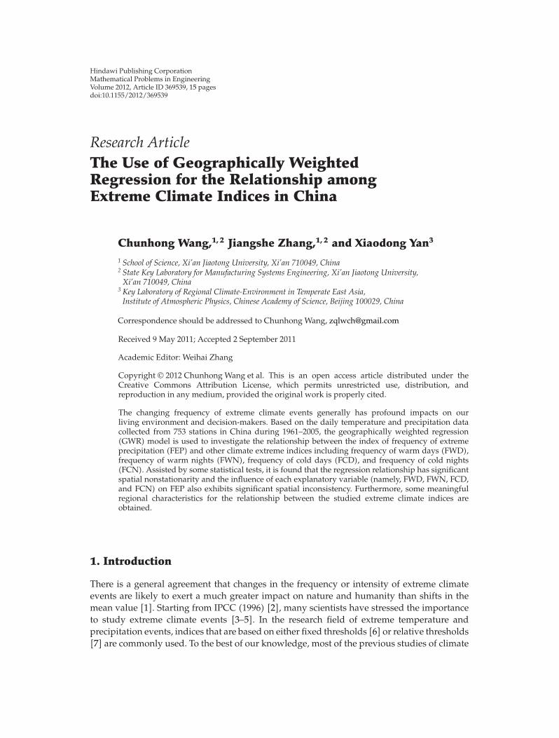
The experimental data sets used in this paper consist of daily maximum and minimumtemperatures and daily precipitation observed at 753 meteorological stations in China fromJanuary 1, 1961 to December 31, 2005, which were offered by National MeteorologicalInformation Center in China Meteorological Administration. Because the study must rely onreliable data, the missing data in each month should be no more than three days. Therefore,the data collected from the 504 stations (Figure 1) which comply with this requirement

Mathematical Problems in Engineering 3

80E 90E 100E 110E 120E 130E

20N

30N

40N

50N

Stations usedStations omitted

Figure 1: Stations for which data were available in China. (•) Stations used in this paper; (+) stationsomitted due to excessive missing data.

were utilized in this work. With respect to the missing values in these 504 stations, a linearinterpolation method was adopted to impute them.

2.2. Extreme Climate Indices

Numerous temperature indices have been used in previous studies of climate events. Someindices involved arbitrary thresholds, such as the number of hot days exceeding 35◦C andsummer days exceeding 25◦C. As indicated byManton et al. [5], these are suitable for regionswith little spatial variability in climate, but arbitrary thresholds are inappropriate for regionsspanning a broad range of climates. In China, climates vary widely from monsoon region inthe eastern part to the westerly region in the northwestern part of the country, so there is nosingle temperature threshold that would be considered an event in all regions. For this reason,some studies have used weather and climate indices based on statistical quantities such asthe 10th (5th) or 90th (95th) percentile [20, 21]; detailed information can be found from theEuropean Climate Assessment & Dataset (ECA&D) Indices List (http://www.knmi.nl/).Upper and lower percentiles of temperature indices are used in all regions, but vary inabsolute magnitude from site to site. A regional climate study in the Caribbean region usingthe same indices can also be found in [21].

As this study covers a broad region in China, climate indices chosen are based onthe 10th and 90th percentiles. The extreme climate indices studied in this paper includeFEP, FWD, FWN, FCD, and FCN whose definitions are described in detail in Table 1. Asfor the experimental data of these extreme indices based on the 1961–1990 base period,the relative values of them were calculated. For each station, the values for FEP, FWD,FWN, FCD, and FCN are their respective values averaged over the period 1961–2005, whichare still denoted as FEP, FWD, FWN, FCD, and FCN in order to facilitate the followingdiscussions.

http://www.knmi.nl/


Table 1: Five extreme climate indices calculated based on daily temperature and precipitation data.

Indicatorname Indicator definition (unit: days)

FEPLet Tpij be the daily precipitation on day i of year j, and let Tpin90 be the calendar day90th percentile centered on a 5-day window for the base period 1961–1990. Frequency ofextreme precipitation (FEP) in year j is the annual count of days when Tpij > Tpin90.

FWDLet Txij be the daily maximum temperature on day i of year j, and let Txin90 be thecalendar day 90th percentile centered on a 5-day window for the base period 1961–1990.Frequency of warm days (FWD) in year j is the annual count of days when Txij > Txin90.

FWNLet Tnij be the daily minimum temperature on day i of year j, and let Tnin90 be thecalendar day 90th percentile centered on a 5-day window for the base period 1961–1990.Frequency of warm nights (FWN) in year j is the annual count of days when Tnij > Tnin90.

FCDLet Txij be the daily maximum temperature on day i of year j, and let Txin10 be thecalendar day 10th percentile centered on a 5-day window for the base period 1961–1990.Frequency of cold days (FCD) in year j is the annual count of days when Txij < Txin10.

FCNLet Tnij be the daily minimum temperature on day i of year j, and let Tnin10 be thecalendar day 10th percentile centered on a 5-day window for the base period 1961–1990.Frequency of cold nights (FCN) in year j is the annual count of days when Tnij < Tnin10.

2.3. Geographically Weighted Regression (GWR)

The technique of linear regression estimates a parameter β that links the explanatory variablesto the response variable. However, when this technique is applied to spatial data, someissues concerning the stationarity of these parameters over the space come out. In “normal”regression, it is generally assumed that the modeling relationship holds everywhere in thestudy area—that is, the regression parameters are “whole-map” statistics. In many situationsthis is not the case, however, as mapping the residuals (the difference between the observedand predicted data) may reveal. The realization in the statistical and geographical sciencesthat a relationship between an explanatory variable and a response variable in a linearregression model is not always constant across a study area has led to the developmentof regression models allowing for spatially varying coefficients. Many different solutionshave been proposed for dealing with spatial variation in the relationship. One of them,developed by Brunsdon et al. [8], has been labelled geographically weighted regression(GWR), which provides an elegant and easily grasped means of modeling such relationshipsby subtly incorporating the spatial characteristics of data via allowing regression coefficientsto depend on some covariates such as longitude and latitude of the meteorological stations.Specifically, it is a nonparametric model of spatial drift that relies on a sequence of locallylinear regressions to produce estimates for every point in space by using a subsample of datainformation from nearby observations. That is to say, this technique allows the modelingof relationships that vary over space by introducing distance-based weights to provideestimates βki for each variable k and each geographical location i. Thus the spatial variationof regression relationship can be effectively analyzed and the inherent disciplines of spatialdata by the estimated coefficients over different locations can be better understood.

An ordinary linear regression (OLR) model can be expressed by

yi = β0 +p∑

j=1

βjxij + εi, i = 1, 2, . . . , n, (2.1)


where yi, i = 1, 2, . . . , n, are the observation of the response variable y, βj(j = 1, 2, . . . , p)represents the regression coefficients, xij is the ith value of the explanatory variable xj , and εiare normally distributed error terms with zero mean and constant variance.

In GWR model, the global regression coefficients are replaced by local parameters

yi = β0(ui, vi) +p∑

j=1

βj(ui, vi)xij + εi, i = 1, 2, . . . , n, (2.2)

where (ui, vi) denotes the longitude and latitude coordinates of the ith meteorological station,(yi;xi1, xi2, . . . , xip) represent the observed value of the response Y and explanatory variablesX1, X2, . . . , Xp at (ui, vi), β0(ui, vi) is the intercept, and βj(ui, vi)(j = 1, 2, . . . , p) are p unknowncoefficient functions of spatial locations, which represent the strength and type of relationshipthat the jth explanatory variable Xj has to the response variable Y . Additionally, ε1, ε2, . . . , εnare error terms which are generally assumed to be independent and identically distributedvariables with mean 0 and common variance σ2. It is worth noticing that the OLR model isactually a special case of the GWR model where βj(ui, vi) are constant for all i = 1, 2, . . . , n.

The coefficient function vector β(ui, vi) for the ith observation in GWR can beestimated via the locally weighted least square procedure [22] as

β(ui, vi) =(β0(ui, vi), β1(ui, vi), . . . , βp(ui, vi)

)T

=(XTW(i)X

)−1XTW(i)Y, i = 1, 2, . . . , n,

βj(u, v) =(βj(u1, v1), βj(u2, v2), . . . , βj(un, vn)

)T, j = 0, 1, 2, . . . , p,

(2.3)

where

X =

⎛⎜⎜⎜⎜⎜⎜⎝

xT1

xT2

...

xTn

⎞⎟⎟⎟⎟⎟⎟⎠

=

⎛⎜⎜⎜⎜⎜⎜⎝

1 x11 · · · x1p

1 x21 · · · x2p

......

...

1 xn1 · · · xnp

⎞⎟⎟⎟⎟⎟⎟⎠

, Y =

⎛⎜⎜⎜⎜⎜⎜⎝

y1

y2

...

yn

⎞⎟⎟⎟⎟⎟⎟⎠

, (2.4)

W(i) = diag[Kh(di1), Kh(di2), . . . , Kh(din)] (2.5)

is a diagonal weight matrix, ensuring that observations near to the location have greaterinfluence than those far away. Here, dij denotes the distance between two observed locations(ui, vi) and (uj, vj), which can be calculated as

dij = R arccos(sin vi sin vj + cos vi cos vj cos

(ui − uj

)), (2.6)


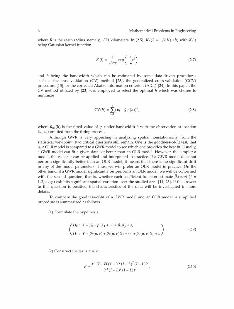
where R is the earth radius, namely, 6371 kilometers. In (2.5), Kh(·) = 1/hK(·/h) with K(·)being Gaussian kernel function

K(t) =1√2π

exp(−12t2)

(2.7)

and h being the bandwidth which can be estimated by some data-driven proceduressuch as the cross-validation (CV) method [23], the generalized cross-validation (GCV)procedure [13], or the corrected Akaike information criterion (AICc) [24]. In this paper, theCV method utilized by [23] was employed to select the optimal h which was chosen tominimize

CV(h) =n∑

i=1

(yi − y(i)(h)

)2, (2.8)

where y(i)(h) is the fitted value of yi under bandwidth h with the observation at location(ui, vi) omitted from the fitting process.

Although GWR is very appealing in analyzing spatial nonstationarity, from thestatistical viewpoint, two critical questions still remain. One is the goodness-of-fit test, thatis, a OLR model is compared to a GWRmodel to see which one provides the best fit. Usually,a GWR model can fit a given data set better than an OLR model. However, the simpler amodel, the easier it can be applied and interpreted in practice. If a GWR model does notperform significantly better than an OLR model, it means that there is no significant driftin any of the model parameters. Thus, we will prefer an OLR model in practice. On theother hand, if a GWR model significantly outperforms an OLR model, we will be concernedwith the second question, that is, whether each coefficient function estimate βj(u, v) (j =1, 2, . . . , p) exhibits significant spatial variation over the studied area [11, 25]. If the answerto this question is positive, the characteristics of the data will be investigated in moredetails.

To compare the goodness-of-fit of a GWR model and an OLR model, a simplifiedprocedure is summarized as follows.

(1) Formulate the hypothesis

⎛

⎝H0 : Y = β0 + β1X1 + · · · + βpXp + ε,

H1 : Y = β0(u, v) + β1(u, v)X1 + · · · + βp(u, v)Xp + ε

⎞

⎠. (2.9)

(2) Construct the test statistic

F =YT (I −H)Y − YT (I − L)T (I − L)Y

YT (I − L)T (I − L)Y. (2.10)


Here, H = X(XTX)−1XT , I is an identity matrix of order n, and

L =

⎛⎜⎜⎜⎜⎜⎜⎜⎝

xT1

(XTW(1)X

)−1XTW(1)

xT2

(XTW(2)X

)−1XTW(2)

...

xTn

(XTW(n)X

)−1XTW(n)

⎞⎟⎟⎟⎟⎟⎟⎟⎠

(2.11)

is an n × n matrix. IfH0 is true, the test statistic F is to be

F =εT

((I −H) − (I − L)T (I − L)

)ε

εT (I − L)T (I − L)ε. (2.12)

(3) Test the hypothesis. The p value should be calculated as

p0 = PH0(F > F0) = PH0

(εT

((I −H) − (1 + F0)(I − L)T (I − L)

)ε > 0

), (2.13)

where F0 is the observed value of F in (2.12). Since it is difficult to derive thenull distribution of F theoretically, the three-moment χ2 approximation procedure[26, 27] devoted to approximate the distribution of normal variable quadratic formsuch as εT ((I − H) − (1 + F0)(I − L)T (I − L))ε was used to compute the p valuedefined in (2.13). Given a significance level α, if p0 < α, the null hypothesis shouldbe rejected. Otherwise, we may conclude that the GWR model cannot improve thefitness significantly in comparison with the OLR model.

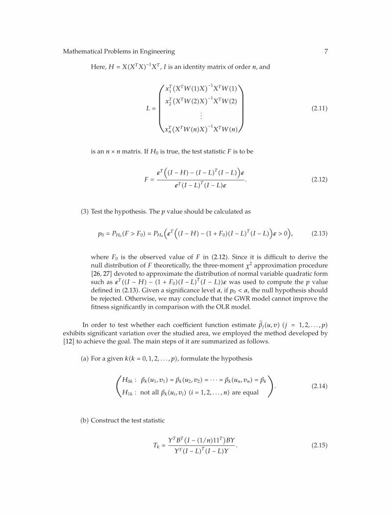
In order to test whether each coefficient function estimate βj(u, v) (j = 1, 2, . . . , p)exhibits significant variation over the studied area, we employed the method developed by[12] to achieve the goal. The main steps of it are summarized as follows.

(a) For a given k(k = 0, 1, 2, . . . , p), formulate the hypothesis

⎛

⎝H0k : βk(u1, v1) = βk(u2, v2) = · · · = βk(un, vn) = βk

H1k : not all βk(ui, vi) (i = 1, 2, . . . , n) are equal

⎞

⎠. (2.14)

(b) Construct the test statistic

Tk =YTBT

(I − (1/n)11T

)BY

YT (I − L)T (I − L)Y. (2.15)


Here, 1 is an n × 1 column vector with unity for each element, and

B =

⎛⎜⎜⎜⎜⎜⎜⎜⎝

eTk+1(XTW(1)X

)−1XTW(1)

eTk+1(XTW(2)X

)−1XTW(2)

...

eTk+1

(XTW(n)X

)−1XTW(n)

⎞⎟⎟⎟⎟⎟⎟⎟⎠

. (2.16)

ek+1 is an n × 1 column vector which takes value 1 for the (k + 1)th element andzero for the other elements. Under the null hypothesis H0k, the test statistic Tk issimplified as

Tk =εTBT

(I − (1/n)11T

)Bε

εT (I − L)T (I − L)ε. (2.17)

(c) Test the hypothesis. The p value is

pk = PH0k(Tk > T0k) = PH0k

(εT

(BT

(I − 1

n11T

)B − T0k(I − L)T (I − L)

)ε > 0

), (2.18)

where T0k is the observed value of Tk in (2.17). Similar to the goodness-of-fit test,the three-moment χ2 approximation procedure was used to derive the p valuedefined in (2.18). Given a significance level α, if pk < α, reject H0k; accept H0k

otherwise.

3. Analysis of Results

In this part, we will carry out numerical experiments for the OLR model and GWR model.All programs are written in Matlab.

3.1. Spatial Distributions of Extreme Climate Indices

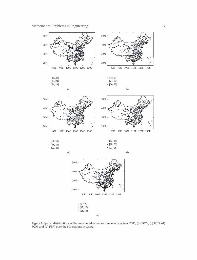
Based on the values of FWD, FWN, FCD, FCN, and FEP, Figure 2 presents the spatialdistributions for each of them over the 504 stations in China.

As shown in Figure 2, FWD, FWN, FCD, FCN, and FEP exhibit some regional features.Generally, there are 16 to 29 times per year for FWD and the larger values for FWD are mainlylocated in the north as well as the east of China. There are 18–35 times per year for FWN. Ifusing the Yangtze River as the boundary, FWN values in the north are generally larger thanthose in the south. As for FCD, there are 14 to 26 times per year. Specially, FCD has smallvalues about 14–18 times per year in most parts of northwest China. With regard to FCN, itis about 13–28 times per year and it has small values in southern China. Furthermore, FEPvalues are between 9 and 33 times per year. In most of the country, its value varies from 25


80E 90E 100E 110E 120E 130E

20N

30N

40N

50N

[16, 20)[20, 24)[24, 29]

(a)

80E 90E 100E 110E 120E 130E

20N

30N

40N

50N

[18, 24)[24, 30)[30, 35]

(b)

80E 90E 100E 110E 120E 130E

20N

30N

40N

50N

[14, 18)[18, 22)[22, 26]

(c)

80E 90E 100E 110E 120E 130E

20N

30N

40N

50N

[13, 18)[18, 23)[23, 28]

(d)

80E 90E 100E 110E 120E 130E

20N

30N

40N

50N

(9, 17)(17, 25)(25, 33)

(e)

Figure 2: Spatial distributions of the considered extreme climate indices ((a) FWD, (b) FWN, (c) FCD, (d)FCN, and (e) FEP) over the 504 stations in China.


Table 2: Correlation coefficients of the independent variables, that is, FWD, FWN, FCD, and FCN.

FWD FWN FCD FCNFWD 1.0000 0.3862 0.3453 0.1836FWN 1.0000 0.1318 0.1329FCD 1.0000 0.4174FCN 1.0000

Table 3:Correlation coefficients of the GWR coefficient estimates, that is, β0(u, v), β1(u, v), β2(u, v), β3(u, v),and β4(u, v).

β0(u, v) β1(u, v) β2(u, v) β3(u, v) β4(u, v)β0(u, v) 1.0000 −0.4068 −0.1734 −0.5044 0.0828β1(u, v) 1.0000 0.0491 −0.3281 −0.0366β2(u, v) 1.0000 −0.4295 0.6309β3(u, v) 1.0000 −0.6375β4(u, v) 1.0000

to 33 times per year, and only in some stations in southern Xinjiang and Tibet, its values liebetween 9 and 17 times per year.

3.2. The Fitted Geographically Weighted Regression Model

In order to make clear the relationship among these extreme climate indices in 504 stations inChina so that some useful information can be provided to decision-makers to help them todeduce the disaster caused by extreme weather, a GWR model was fitted by consideringFEP as the response variable Y and FWD, FWN, FCD, and FCN as the explanatoryvariables (X1, X2, X3, X4), respectively. Letting n be equal to 504 and p equal to 4 and letting(yi, xi1, xi2, xi3, xi4) be the observations of the variables (Y,X1, X2, X3, X4) at the location(ui, vi), the model (2.2) can be expressed as

yi = β0(ui, vi) +4∑

j=1

βj(ui, vi)xij + εi, i = 1, 2, . . . , 504, (3.1)

based on the data collected from the 504 stations.When we apply a fixed Gaussian function, the minimum score of (2.8) is obtained

when the bandwidth h equals approximately 240 km. Thus, the weighting matrix W(i) isestimated, where wij = (1/(240 ∗ √

2π)) exp(−d2ij/(2 ∗ 2402)). Based on (2.3), βj(u, v)(j =

0, 1, 2, 3, 4) are calculated by the locally weighted least square approach. Hence, the strengthand type of relationship that FWD (FWN, FCD, FCN) has with FEP over 504 stations in Chinacan be studied.

Because Wheeler [28–30] raised the multicollinearity issues, correlation coefficients ofthe independent variables as well as that of the GWR coefficient estimates were presented inTables 2 and 3, respectively.


0 100 200 300 400 500 600−15

−10

−5

0

5

10

Stations

Pred

iction

error(P

E)

PE OLRPE GWR

std(PE OLR) = 2.9401

std(PE GWR) = 1.3039

Figure 3: Prediction error (PE) of the responsible variable, FEP, for ordinary linear regression (OLR) andgeographically weighted regression (GWR) over the 504 stations in China.

As shown in Tables 2 and 3, correlation coefficients of the independent variablesas well as that of the GWR coefficient estimates are all not large, except for that betweenβ2(u, v) and β4(u, v), as well as β3(u, v) and β4(u, v), whose absolute values are more than0.5. It indicates that β4(u, v) has a positive correlation with β2(u, v), while it has a negativecorrelation with β3(u, v). We ignore the correlation between the independent variables in thispaper.

After conducting the goodness-of-fit test, the computed p value is smaller thanthe significance level 0.05. Thus, the GWR model can describe the regression relationshipsignificantly better than the OLR model and it indicates that the relationship between FEPand FWD, FWN, FCD, and FCN has spatial nonstationarity. Define

R2 =∑504

i=1(yi − y

)2∑504

i=1(yi − y

)2 (3.2)

to measure the goodness of fit of the regression relationship on the given data set. The R2

values for the OLR and GWR model are 0.3953 and 0.7750, respectively, which indicatesthat the GWR model can capture a larger amount (77.50%) of variance of FEP based on theclimate indices FWD, FWN, FCD, and FCN, than the OLR model. The prediction errors (i.e.,residual errors) for the OLR and GWR model are presented in Figure 3, which shows theprediction error of the GWRmodel and its standard error are both lower than that of the OLRmodel.

Furthermore, the statistical significance tests for the variations of the coefficient func-tions are carried out. The obtained results show that all the regression coefficient estimates


Table 4: p value of relevant tests for the GWR model (3.1).

Globalstationarity forregressionrelationship

Significance forβ0(u, v)





0 1.4816 ∗ 10−6 0 0.0018 0 1.5184 ∗ 10−6

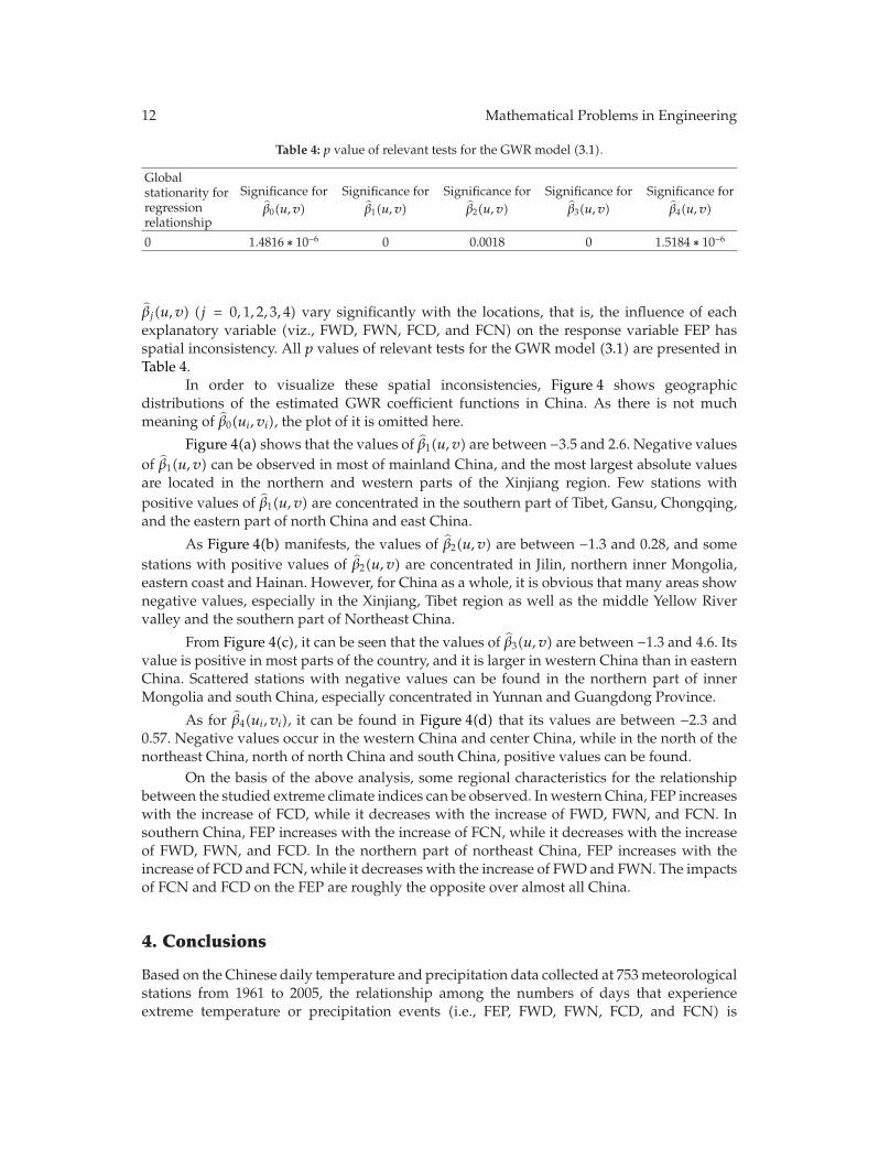
βj(u, v) (j = 0, 1, 2, 3, 4) vary significantly with the locations, that is, the influence of eachexplanatory variable (viz., FWD, FWN, FCD, and FCN) on the response variable FEP hasspatial inconsistency. All p values of relevant tests for the GWR model (3.1) are presented inTable 4.

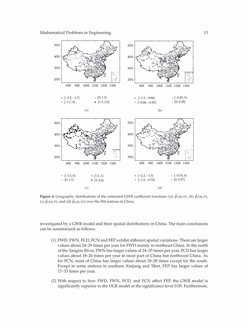
In order to visualize these spatial inconsistencies, Figure 4 shows geographicdistributions of the estimated GWR coefficient functions in China. As there is not muchmeaning of β0(ui, vi), the plot of it is omitted here.

Figure 4(a) shows that the values of β1(u, v) are between −3.5 and 2.6. Negative valuesof β1(u, v) can be observed in most of mainland China, and the most largest absolute valuesare located in the northern and western parts of the Xinjiang region. Few stations withpositive values of β1(u, v) are concentrated in the southern part of Tibet, Gansu, Chongqing,and the eastern part of north China and east China.

As Figure 4(b) manifests, the values of β2(u, v) are between −1.3 and 0.28, and somestations with positive values of β2(u, v) are concentrated in Jilin, northern inner Mongolia,eastern coast and Hainan. However, for China as a whole, it is obvious that many areas shownegative values, especially in the Xinjiang, Tibet region as well as the middle Yellow Rivervalley and the southern part of Northeast China.

From Figure 4(c), it can be seen that the values of β3(u, v) are between −1.3 and 4.6. Itsvalue is positive in most parts of the country, and it is larger in western China than in easternChina. Scattered stations with negative values can be found in the northern part of innerMongolia and south China, especially concentrated in Yunnan and Guangdong Province.

As for β4(ui, vi), it can be found in Figure 4(d) that its values are between −2.3 and0.57. Negative values occur in the western China and center China, while in the north of thenortheast China, north of north China and south China, positive values can be found.

On the basis of the above analysis, some regional characteristics for the relationshipbetween the studied extreme climate indices can be observed. Inwestern China, FEP increaseswith the increase of FCD, while it decreases with the increase of FWD, FWN, and FCN. Insouthern China, FEP increases with the increase of FCN, while it decreases with the increaseof FWD, FWN, and FCD. In the northern part of northeast China, FEP increases with theincrease of FCD and FCN, while it decreases with the increase of FWD and FWN. The impactsof FCN and FCD on the FEP are roughly the opposite over almost all China.

4. Conclusions

Based on the Chinese daily temperature and precipitation data collected at 753meteorologicalstations from 1961 to 2005, the relationship among the numbers of days that experienceextreme temperature or precipitation events (i.e., FEP, FWD, FWN, FCD, and FCN) is


80E 90E 100E 110E 120E 130E

20N

30N

40N

50N

[−3.5, −1.7)[−1.7, 0)

[0, 1.3)[1.3, 2.6]

(a)

80E 90E 100E 110E 120E 130E

20N

30N

40N

50N

[−1.3, −0.86)[−0.86, −0.43)

[−0.43, 0)[0, 0.28]

(b)

80E 90E 100E 110E 120E 130E

20N

30N

40N

50N

[−1.3, 0) [1.5, 3)[3, 4.6][0, 1.5)

(c)

80E 90E 100E 110E 120E 130E

20N

30N

40N

50N

[−2.3, −1.5)[−1.5, −0.74)

[−0.74, 0)[0, 0.57]

(d)

Figure 4: Geographic distributions of the estimated GWR coefficient functions ((a) β1(u, v), (b) β2(u, v),(c) β3(u, v), and (d) β4(u, v)) over the 504 stations in China.

investigated by a GWR model and their spatial distributions in China. The main conclusionscan be summarized as follows.

(1) FWD, FWN, FCD, FCN and FEP exhibit different spatial variations. There are largervalues about 24–29 times per year for FWDmainly in northeast China. In the northof the Yangtze River, FWN has larger values of 24–35 times per year. FCD has largervalues about 18–26 times per year in most part of China but northwest China. Asfor FCN, most of China has larger values about 18–28 times except for the south.Except in some stations in southern Xinjiang and Tibet, FEP has larger values of17–33 times per year.

(2) With respect to how FWD, FWN, FCD, and FCN affect FEP, the GWR model issignificantly superior to the OLR model at the significance level 0.05. Furthermore,


the statistical tests indicate that the influence of each explanatory variable (viz.,FWD, FWN, FCD, and FCN) on FEP has spatial inconsistency.

(3) Some regional features are detected for the relationship between the studied ex-treme climate indices. In western China, FCD has a positive effect on FEP, which iscontrary to that of FWD, FWN, and FCN. However, it is just the opposite in south-ern China. The effects of FCD as well as FCN on FEP are positive in the northernpart of Northeast China, while those of FWD and FWN are negative. Meanwhile,FCN and FCD have the opposite influence on FEP over most of China.

Acknowledgments

This work is supported by the National Natural Science Foundation of China (Grant nos.60675013, 10531030) and the National Basic Research Program of China (973 Program) (Grantno. 2007CB311002).

References

[1] R. W. Katz and B. G. Brown, “Extreme events in a changing climate: variability is more importantthan averages,” Climatic Change, vol. 21, no. 3, pp. 289–302, 1992.

[2] J. T. Houghton, L. G. M. Filho, B. A. Callander, N. Harris, A. Kattenberg, and K. Maskell, Eds., ClimateChange 1995: The Science of Climate Change. Contribution of Working Group I to the Second AssessmentReport of the Intergovernmental Panel on Climate Change, Cambridge University Press, Cambridge, UK,1996.

[3] T. R. Karl, N. Nicholls, and A. Ghazi, “CLIVAR/GCOS/WMO Workshop on Indices and Indicatorsfor climate extremes,” Climatic Change, vol. 42, no. 1, pp. 3–7, 1999.

[4] C. K. Folland, C. Miller, D. Bader et al., “”Workshop on indices and indicators for climate extremes,asheville, NC, USA, 3–6 June 1997, breakout group C: temperature indices for climate extremes,”Climatic Change, vol. 42, no. 1, pp. 31–41, 1999.

[5] M. J. Manton, P. M. Della-Marta, M. R. Haylock et al., “Trends in extreme daily rainfall andtemperature in southeast Asia and the south Pacific: 1961–1998,” International Journal of Climatology,vol. 21, no. 3, pp. 269–284, 2001.

[6] B. D. Su, T. Jiang, and W. B. Jin, “Recent trends in observed temperature and precipitation extremesin the Yangtze River basin, China,” Theoretical and Applied Climatology, vol. 83, no. 1–4, pp. 139–151,2006.

[7] P. Zhai, A. Sun, F. Ren, X. Liu, B. Gao, and Q. Zhang, “Changes of climate extremes in China,” ClimaticChange, vol. 42, no. 1, pp. 203–218, 1999.

[8] C. Brunsdon, A. S. Fotheringham, and M. E. Charlton, “Geographically weighted regression: amethod for exploring spatial nonstationarity,” Geographical Analysis, vol. 28, no. 4, pp. 281–298, 1996.

[9] A. S. Fotheringham, M. Charlton, and C. Brunsdon, “The geography of parameter space: aninvestigation of spatial non-stationarity,” International Journal of Geographical Information Systems,vol. 10, no. 5, pp. 605–627, 1996.

[10] C. Brunsdont, S. Fotheringham, and M. Charlton, “Geographically weighted regression: modellingspatial non-stationarity,” Journal of the Royal Statistical Society Series D, vol. 47, no. 3, pp. 431–443, 1998.

[11] Y. Leung, C. L. Mei, and W. X. Zhang, “Statistical tests for spatial nonstationarity based on thegeographically weighted regression model,” Environment and Planning A, vol. 32, no. 1, pp. 9–32,2000.

[12] Y. Leung, C. L. Mei, and W. X. Zhang, “Testing for spatial autocorrelation among the residuals of thegeographically weighted regression,” Environment and Planning A, vol. 32, no. 5, pp. 871–890, 2000.

[13] A. Fotheringham, C. Brunsdon, and M. Charlton, Geographically Weighted Regression: The Analysis ofSpatially Varying Relationships, Wiley, Chichester, UK, 2002.

[14] V. Huang and Y. Leung, “Analysing regional industrialisation in Jiangsu province using geographi-cally weighted regression,” Journal of Geographical Systems, vol. 4, no. 2, pp. 233–249, 2002.


[15] P. A. Longley and C. Tobon, “Spatial dependence and heterogeneity in patterns of hardship: an intra-urban analysis,” Annals of the Association of American Geographers, vol. 94, no. 3, pp. 503–519, 2004.

[16] T. Nakaya, “Local spatial interaction modelling based on the geographically weighted regressionapproach,” GeoJournal, vol. 53, no. 4, pp. 347–358, 2001.

[17] W. Qian and Y. Zhu, “Climate change in China from 1880 to 1998 and its impact on the environmentalcondition,” Climatic Change, vol. 50, no. 4, pp. 419–444, 2001.

[18] W. Qian, L. Quan, and S. Shi, “Variations of the dust storm in China and its climatic control,” Journalof Climate, vol. 15, no. 10, pp. 1216–1229, 2002.

[19] W. Qian, H. S. Kang, and D. K. Lee, “Distribution of seasonal rainfall in the East Asian monsoonregion,” Theoretical and Applied Climatology, vol. 73, no. 3-4, pp. 151–168, 2002.

[20] T. C. Peterson, M. A. Taylor, R. Demeritte et al., “Recent changes in climate extremes in the Caribbeanregion,” Journal of Geophysical Research D, vol. 107, no. 21, p. 4601, 2002.

[21] N. Plummer, M. J. Salinger, N. Nicholls et al., “Changes in climate extremes over the Australian regionand New Zealand during the twentieth century,” Climatic Change, vol. 42, no. 1, pp. 183–202, 1999.

[22] C. Brunsdon, A. S. Fotheringham, and M. Charlton, “Some notes on parametric significance tests forgeographically weighted regression,” Journal of Regional Science, vol. 39, no. 3, pp. 497–524, 1999.

[23] L. Desmet and I. Gijbels, “Local linear fitting and improved estimation near peaks,” The CanadianJournal of Statistics, vol. 37, no. 3, pp. 453–475, 2009.

[24] C. M. Hurvich, J. S. Simonoff, and C.-L. Tsai, “Smoothing parameter selection in nonparametricregression using an improved Akaike information criterion,” Journal of the Royal Statistical Society B,vol. 60, no. 2, pp. 271–293, 1998.

[25] C. Brunsdon, M. Aitkin, S. Fotheringham, and M. Charlton, “A comparison of random coefficientmodelling and geographically weighted regression for spatially non-stationary regression problems,”Geographical and Environmental Modelling, vol. 3, no. 1, pp. 47–62, 1999.

[26] C. L. Mei and W. X. Zhang, “Testing linear regression relationships via locally-weighted-fittingtechnique,” Journal of Systems Science and Mathematical Sciences, vol. 22, no. 4, pp. 467–480, 2002.

[27] C.-h. Wei and X.-z. Wu, “Testing linearity for nonparametric component of partially linear models,”Mathematica Applicata, vol. 20, no. 1, pp. 183–190, 2007.

[28] D. Wheeler and M. Tiefelsdorf, “Multicollinearity and correlation among local regression coefficientsin geographically weighted regression,” Journal of Geographical Systems, vol. 7, no. 2, pp. 161–187, 2005.

[29] D. C. Wheeler, “Diagnostic tools and a remedial method for collinearity in geographically weightedregression,” Environment and Planning A, vol. 39, no. 10, pp. 2464–2481, 2007.

[30] D. C. Wheeler, “Simultaneous coefficient penalization and model selection in geographicallyweighted regression: the geographically weighted lasso,” Environment and Planning A, vol. 41, no. 3,pp. 722–742, 2009.

Submit your manuscripts athttp://www.hindawi.com

Hindawi Publishing Corporationhttp://www.hindawi.com Volume 2014

MathematicsJournal of


Mathematical Problems in Engineering

Hindawi Publishing Corporationhttp://www.hindawi.com

Differential EquationsInternational Journal of

Volume 2014

Applied MathematicsJournal of


Probability and StatisticsHindawi Publishing Corporationhttp://www.hindawi.com Volume 2014

Journal of


Mathematical PhysicsAdvances in

Complex AnalysisJournal of


OptimizationJournal of


CombinatoricsHindawi Publishing Corporationhttp://www.hindawi.com Volume 2014

International Journal of


Operations ResearchAdvances in

Journal of


Function Spaces

Abstract and Applied AnalysisHindawi Publishing Corporationhttp://www.hindawi.com Volume 2014

International Journal of Mathematics and Mathematical Sciences


The Scientific World JournalHindawi Publishing Corporation http://www.hindawi.com Volume 2014


Algebra

Discrete Dynamics in Nature and Society



Decision SciencesAdvances in

Discrete MathematicsJournal of

Hindawi Publishing Corporationhttp://www.hindawi.com

Volume 2014 Hindawi Publishing Corporationhttp://www.hindawi.com Volume 2014

Stochastic AnalysisInternational Journal of

Documents

Research Article The Use of Geographically Weighted - downloads