Research Coupling PV and CAES Power Plants to Transform ... · Plants to Transform Intermittent PV Electricity into a Dispatchable ... combined-cycle ... PV mounting supports, grounding

PROGRESS IN PHOTOVOLTAICS: RESEARCH AND APPLICATIONS

Prog. Photovolt: Res. Appl. 2008; 16:649–668

Published online 6 October

* Correspondence to: JamesInstitute, 52 Columbia StreeyE-mail: je_mason@verizon.

Copyright # 2008 John Wil

2008 in Wiley InterScience (www.interscience.wiley.com) DOI: 10.1002/pip.858

Research

Coupling PV and CAES PowerPlants to Transform IntermittentPV Electricity into a Dispatchable
Electricity Source James Mason1*,y, Vasilis Fthenakis2, Ken Zweibel3, Tom Hansen4 and Thomas Nikolakakis5
1Renewable Energy Research Institute, 52 Columbia Street, Farmingdale, NY 17735, USA2Center for Life Cycle Analysis, Columbia University, and Director of PV EH&S Research Center, Brookhaven National Laboratory, Upton, NY 11973, USA3Institute for the Analysis of Solar Energy, George Washington University, 2121 I St. NW, Washington, DC 20052, USA4Tucson Electric Power, P.O. Box 711, Tucson, AZ 85702, USA5Center for Life Cycle Analysis, Columbia University, 2960 Broadway, New York City, NY 10027, USA

This study investigates the transformation of photovoltaic (PV) electricity production from an intermittent

into a dispatchable source of electricity by coupling PV plants to compressed air energy storage (CAES) gas

turbine power plants. Based on historical solar irradiation data for the United States’ south western states and

actual PV and CAES performance data, we show that the large-scale adoption of coupled PV–CAES power

plants will likely enable peak electricity generation in 2020 at costs equal to or lower than those from natural

gas power plants with or without carbon capture and storage systems. Our findings also suggest that given

the societal value of reducing carbon dioxide and the sensitivity of conventional generation to rising fossil

fuel prices, this competitive crossover point may occur much sooner. Copyright # 2008 John Wiley &

Sons, Ltd.

key words: photovoltaics; CAES; solar energy

Received 1 February 2008; Revised 31 July 2008

INTRODUCTION

Since 1978, compressed air energy storage (CAES)

plants have been in service to store excess off-peak

electricity in the form of compressed air for use during

peak load times. The original idea for CAES power

plants was to utilize inexpensive, off-peak electricity to

pressurize air at CAES plants, and to store the

compressed air in underground reservoirs.1 The stored

Mason, Renewable Energy Researcht, Farmingdale, NY 17735, USA.net

ey & Sons, Ltd.

compressed air can then be released on demand to the

CAES plant’s turbo-generator set to generate premium

value electricity. The first CAES plant was built in

Huntorf (Germany) in 1978.

The conceptualization of CAES was broadened in the

1990s as a means of solving the intermittency of wind

turbine electricity production. Beginning with Cavallo,2

numerous studies have explored the economic feasibility

of coupling wind farms and CAES gas turbine (GT)

power plants for base load electricity production.3–8 The

basic idea of these studies is to locate underground

storage facilities in relative proximity to the wind farms

and to use the CAES plants to firm and shape the

intermittency of wind electricity production.

1It should be noted that we do not model tracking systems for PVplants, which would increase the average annual capacity factor toapproximately 40% with two-axis trackers, and that we do not modelan HVDC system that integrates the flow of Southwest PVelectricityproduction with the flow of Southwest or Midwest wind electricityproduction, which may be another means of increasing the HVDCtransmission capacity utilization factor. Both of these issues areimportant, but due to data constraints are beyond the scope of thisanalysis. This study is the first in hopefully an emerging body ofstudies that will investigate a variety of models for PV electricityproduction in the Southwest US.

650 J. MASON ET AL.

The wind studies demonstrate that areas of the

country with high wind regimes are highly correlated

with potential aquifer air storage reservoirs, which

enable the location of CAES plants in close proximity

to wind farms to alleviate transmission bottlenecks

and the need for transmission system additions and

upgrades.8 The electricity from both wind farms and

CAES plants are gathered for distribution to local

markets via high voltage direct current (HVDC) power

lines. The ability to locate CAES plants in close

proximity to wind farms facilitates the bundling of

wind and CAES electricity for long-distance trans-

mission via HVDC power lines, which increases the

capacity utilization factor of the HVDC lines from

35% for wind only electricity to 90% for wind plus

CAES electricity and lowers transmission cost.

This study extends CAES research by investigating

the application of CAES to resolve the intermittency of

photovoltaic (PV) electricity production. We concep-

tualize CAES as a means of storing PV electricity that

is produced in the high solar insolation areas of the

Southwest US. The idea is to transport PV electricity

from the Southwest to local markets throughout the US

via HVDC power lines. A CAES plant is located in

close proximity to the DC–AC converter station at the

connection point to the local AC electricity distribution

system. A portion of the PV electricity is sent to the

CAES plant and stored in the form of compressed air.

The CAES plant utilizes the stored compressed air

to generate electricity on demand to transform the

intermittent PV electricity into dispatchable peak and

base load electricity for the local market.

The CAES plant serves three basic functions. For

one, the CAES plant firms and shapes the portion of

PV electricity consigned to grid distribution. Sec-

ondly, the CAES plant maintains a desired level of

controlled electricity production capacity over the

scheduled electricity production period. And thirdly,

the CAES plant provides firm capacity value to a very

large potential source of PV electrical energy in the

US.

Our modeling of coupled PV CAES plants differs

from coupled wind CAES systems in that PV plants are

not necessarily located in close proximity to CAES

plants. PV plants are located in the high insolation

Southwest US, which has an average insolation of

6�4 kWh m�2 day�1. This Southwest average insolation

level translates into a 26�7% average annual capacity

factor for PV power plants. The low annual capacity factor

of PV power plants results in a low capacity utilization

factor for the dedicated HVDC power lines, which

Copyright # 2008 John Wiley & Sons, Ltd.

increases transmission costs and the number of power

transmission lines.1

There are two basic reasons for not modeling PV

plants in close proximity to CAES plants. For one,

water is scarce in the arid Southwest, and CAES GT

power plants require substantial amounts of cooling

water. And the second is the limited availability of air

storage reservoirs in the suitable regions of the

Southwest US, which implies that at high PV

penetration levels there will not be the ability to

locate CAES plants in close proximity to PV plants.

We model PV–CAES plants for both peak and base

load operations. Peak PV–CAES plants are designed to

produce 110 MW of power, 10-h d�1, Monday–Friday,

throughout the year. Base load PV–CAES plants are

designed to produce 400 MW of power, 24-h d�1,

throughout the year, with a 90% annual availability.

Our simulations are based on actual performance

parameters of current PV and CAES systems and

forecasts of near-term costs.9–11

The study evaluates levelized cost of electricity

(LCOE), fuel consumption, and carbon dioxide (CO2)

emissions. The findings for PV–CAES plants are

compared to conventional GT plants, natural gas

combined-cycle (NGCC) plants, and coal integrated

gasification combined-cycle (IGCC) plants. The

NGCC and coal IGCC plants are modeled with carbon

capture and storage (CCS) systems to enable the

comparison of low CO2 emissions PV–CAES power

plants to low CO2 emissions fossil fuel power plants.

The research is important because it addresses the

concern of electric utilities that increasing amounts of

time variant PV electricity generation connected to the

nation’s electrical grid could in time adversely impact

reliability. Another reason this study is important is

that it investigates a means of decreasing natural gas

consumption for electricity production, which reduces

both CO2 emissions and demand for limited US natural

gas reserves. The research is timely because of recent

decreases in PV cost from the advent of second-

generation, thin film PV.


DOI: 10.1002/pip

COUPLING PV AND CAES POWER PLANTS 651

The study is organized as follows. The following

section develops an electricity production profile for

PV power plants located in the Southwest US. The

third section describes CAES power plants. Following

this is a section on peak PV–CAES plants, which

includes a comparison to peak fossil fuel plants. The

fifth section presents the base load PV–CAES model

with a comparison to fossil fuel plants with CCS

systems. The final section summarizes findings.

2Ongoing PV research suggests the potential for other PV technol-ogies such as crystalline silicon (c-Si), amorphous silicon (a-Si),copper–indium–gallium–selenium (CIGS), and gallium arsenideconcentrator PV technologies to match the projected 2020 cost ofelectricity estimates for CdTe thin film PV. Our projections are basedon CdTe thin film PV because its development history providesrelatively high confidence in future cost and performanceprojections.

ELECTRICITY PRODUCTION BY PVPOWER PLANTS LOCATED IN THESOUTHWEST US

The first task is to establish an electricity production

profile for central PV power plants located in the

Southwest US. Electricity production by PV power

plants is estimated by applying the historical insolation

records from the National Solar Radiation Data Base

(NSRDB).12,13 The NSRDB contains a 45-year, 1961–

2005, record of insolation measurements. The NSRDB

insolation records used in this study are for six

locations distributed across the Southwest US—

Phoenix, Tucson, Albuquerque, El Paso, Las Vegas,

and Daggett.

Insolation records for the six selected sites are

averaged to create a daily Southwest insolation

estimate for each of the 45 years. This generates a

45-year record of average daily insolation in the

geographically suitable areas of the Southwest. The

insolation record provides us with information to

model the effect of both intra- and inter-annual

variation in insolation on PV electricity production

levels.

It is assumed that PV plants are composed of flat-

plate PV modules facing south and tilted at an angle

equal to the site’s latitude. A combination of daily and

monthly NSRDB global insolation records are

employed to estimate PV electricity production due

to NSRDB data reporting constraints. The daily

NSRDB insolation records, which are measured in

hourly increments, contain data for global insolation

striking a horizontal surface; these are converted to

insolation on latitude-tilted surfaces.14 The conversion

of daily global insolation on horizontal surfaces to

daily global insolation on latitude-tilted surfaces is

based on the extrapolation of daily insolation adjust-

ment factors generated from the measurement of

changes in the monthly insolation records for latitude-

tilted surfaces.


The components of PV power plants are PV modules

and balance of plant components, which include land,

site preparation, PV mounting supports, grounding

system, wiring, transformers, and construction. PV

plants producing DC electricity for grid distribution

are assumed to have 85% system efficiency15 and 99%

availability.16 We also account for 0�5% per annum

losses due to PV module soiling and degradation, and

we model the addition of PVarrays each year as part of

the standard PV plant operating and maintenance

schedule to compensate the soiling and degradation

losses. In other words, we maintain a constant PV

production level despite PV electricity losses due to

annual soiling and PV module degradation.

PV cost and performance parameters are presented

in Table I. PV power plant capital cost estimates are

presented for 2007, 2015, and 2020 to take into account

the projected development of thin film PV. The capital

costs for PV power plants utilizing lowest cost PV

components were $4200 kW�1 in 2007.17 In 2008,

Southern California Edison announced it was con-

tracting for thin film PV at $3500 kW�1 for rooftop

installations and for the California Market Referent

price of 12 ¢ kWh�1, after solar incentives, for a large,

ground-mounted system.18 We estimate future PV

power plant capital costs of $2000 kW�1 in 2015 and

$1300 kW�1 in 2020. The projected PV cost reductions

are expected through a combination of technical

advances and the realization of optimized scale

economies in material flows in both PV manufacturing

and installation.19,20

The PV technology employed for this study is

cadmium telluride (CdTe) thin film PV patterned after

First Solar’s module product,21 which at present is the

lowest cost PV module technology.2 Since CdTe thin

film PV is a new technology, its technological progress

is rapid. Also, increases in the manufacturing scale of

PV modules will further reduce PV module costs. The

balance of plant costs and operating expenses for PV

power plants are based on the German Juwi Group

40 MW plant and the Tucson Electric Power Spring-

erville 4�6 MW PV plant.10,17 As with PV module

costs, balance of plant costs are expected to decline


DOI: 10.1002/pip

Table I. PV–CAES and GT peak power plant cost and performance assumptions�

(Constant 2007 $ US) 2007 2015 2020 Reference

Capital costs

PV modules ($ kW�1) 2 200 1 000 650 40

PV balance of plant ($ kW�1) 1 800 1 000 650 40

CAES turbo-generator set ($ kW�1) 190 190 190 37

CAES compressor ($ kW�1)y 175 175 175 37

CAES peak balance of plant ($ kW�1) 230 230 230 33

CAES-base load balance of plant ($ kW�1)� 139 139 139 33

CAES peak compressor/turbine power ratio 1�09 1�09 1�09

CAES-base load compressor/turbine power ratio 2�21 2�21 2�21

CAES air storage reservoir ($ kWh�1)� 2�00 2�00 2�00

NG GT plant ($ kW�1) 485 485 485 11

HVDC overhead lines ($ km�1) 485 000 485 000 485 000 22

HVDC converter station (million $/station) 475 475 475 22

Performance assumptions and costs

PV plant system efficiency 0�85 0�85 0�85 15

PV plant operational availability 0�99 0�99 0�99 40

PV O&M ($ per year) 750 000 750 000 750 000 40

PV plant annual capacity factor 26�7% 26�7% 26�7% 40

Average Southwest insolation (kWh m�2 day�1) 6�4 6�4 6�4 13

Transmission losses (per 2400 km) 0�06 0�06 0�06 22

HVDC DC–AC conversion efficiency (%) 0�99 0�99 0�99 22

Power connection to compressors (%)z 0�97 0�97 0�97

CAES plant energy ratio (kWhin/kWhout) 0�84 0�84 0�84

CAES peak plant heat rate (MJ kWh�1) 5�064 5�064 5�064

CAES-base load plant heat rate (MJ kWh�1) 4�819 4�819 4�819

CAES plant fixed O&M ($ kW�1) 3�69 3�69 3�69 11

CAES plant variable O&M ($ kWh�1) 0�006 0�006 0�006 11

CAES parasitic power loss (% of output) 2% 2% 2%

NG GT heat rate (MJ kWh�1) 12�24 12�24 12�24 11

NG GT fixed O&M ($ kW�1) 20�3 20�3 20�3 11

NG GT variable O&M ($ kWh�1) 0�0043 0�0043 0�0043 11

NG GT parasitic power loss (% of output) 2% 2% 2%

Notes:�All dollar amounts are presented in constant 2007 $. If the reference is blank, then the data entry is original to this study. Heat rates are

reported at the fuel’s high heat value.yThe compressor cost estimate is the baseline cost stated in terms of $ kW�1 of turbine power output and needs to be scaled by the

compressor/turbine power ratio to establish the actual compressor cost for the peak and base load CAES plants.zWe assume 3% electricity losses at the compressor station due to low electricity flow levels that are not sufficient to meet the compressors

minimum power requirements. This electricity loss rate is not based empirical data but is included as a conservative loss factor.

652 J. MASON ET AL.

with increased module output per unit area, i.e.,

increases in PV efficiency, scale economies in the

manufacture and purchase of balance of plant

components, and technical progress.

On a final note, a national electricity transmission

system is required to transport the large quantities of

PVelectricity from remote Southwest locations to local

markets throughout the US. Therefore, an HVDC

transmission system is included as an integral

component of the PV electricity production and

distribution system. We project a 6% electricity loss


for the average 2400 km transmission distance between

PV plants and distributed CAES plants over the HVDC

transmission network.22 An additional 1% electricity

loss is modeled for the conversion of DC to AC

electricity at the DC–AC converter stations.22 We

model three DC-AC converter stations per 2400 km of

the HVDC transmission system. The estimated

levelized cost of HVDC electricity transmission is

$0�024 kWh�1 and is derived from the HVDC cost and

performance parameters in Table I, the financial

parameters in Table II, and a 26�7% HVDC capacity


DOI: 10.1002/pip

Table II. Financial assumptions to estimate cost of electricity�

Construction periody Three years

Capital payments: three equal payments Three equal payments

Ratio of equity capital to debt capital 45% Equity/55% debt

Nominal return on equity 10�0% Per Year

Nominal return on debt 6�5% Per Year

Real capital charge rate (weighted average cost of capital) 5�0%

Annual inflation rate 1�9%

Property tax and insurance (CAES plant) 2% Of initial capital per year

Property tax and insurance (PV plant)z 1% Of initial capital per year

Working capital 15% Of annual change in expenses

Depreciation MACRS

Corporate tax rate 38�20%

Replacement cost (occurring in years 10 and 20) 5% Of initial capital

30-Year book life; 20-year tax life

Notes:�The LCOE estimates are calculated by the net present value cash flow method.41

yPV installation is incremental, which means that revenues can be generated during the construction period. The three-year construction

period is for construction of the CAES GT plant and the air storage reservoir.zInsurance rate is assumed to be 0�5% of initial capital since insurance is required only for PV modules. Property tax is assumed to be 0�5% of

initial capital since PV plants are located in the largely unpopulated Southwest US.


utilization factor for the distribution of PV electricity

from the Southwest.3

The development of an HVDC electricity trans-

mission system out of the Southwest and spanning the

US will require national level planning and imple-

mentation. At present, it is very difficult to gain right-

of-ways for long-distance power lines. Assuming a 5–7

gigawatt (GW) capacity for HVDC power lines,23,24

approximately 200 HVDC power lines will be required

to transport a terawatt of PV power capacity. While the

development of a HVDC transmission system to

support super large-scale Southwest PV electricity

production will present challenges, it is doable.24,25

The sizing of HVDC power lines has to accommo-

date the peak electricity production of PV’s power

capacity, which occurs for only a brief period each day.

The inherent daily profile of PV electricity production

means that dedicated HVDC lines are underutilized. To

address concerns over the low capacity utilization of a

costly HVDC system, an abbreviated analysis of an

alternative system composed of distributed PV–CAES

plants, where the PVand CAES plants are built in close

proximity to one another throughout the country, is

performed to assess the economic efficacy of the

Southwest PV and distributed CAES model.

3If only one DC–AC converter station is required for the 2400 kmHVDC line, then the levelized cost of electricity transmission is$0.016 kWh with a 26.7% capacity utilization factor.


Another possibility that we did not model is to

simply build distributed PV fields linked to peak

natural gas plants to shape and firm the PV electricity.

However, this would be similar to the use of standby

reserve capacity of natural gas plants, which results in

more fuel consumption and CO2 emissions than PV–

CAES plants. Other HVDC combinations could also

be studied, e.g., PV–CAES with higher capacity factor

from tracking PV; PV combined with wind, which can

be quite complementary and allows for much higher

capacity factors than either alone. On a final note,

intercontinental HVDC is also possible with the

potential to raise capacity use to over 50% for solar

alone, but such long lines have very high expenses and

many other challenges.

CAES POWER PLANTS

CAES GT power plants are similar to conventional GT

power plants with the key exception that air

compressors are separated from the turbo-generator

set. The turbo-generator set consists of a high- and low-

pressure expander-turbine units and electricity gen-

erators. In conventional GT plants, a single shaft

connects the compressors and turbo-generator train,

and the energy to compress air consumes approxi-

mately two-thirds of the energy generated by the

turbine. In the CAES plant design, the separation of

compressors from the turbo-generator set enables all of


DOI: 10.1002/pip

654 J. MASON ET AL.

the turbine’s mechanical energy to be used for

electricity generation, which triples the turbine’s

electricity generation capacity.

CAES power plants use an external source of

electricity to provide the energy for air compression.

The compressed air is then stored in underground

reservoirs. The stored compressed air is released on

demand to provide kinetic energy to power the plant’s

turbines. Suitable underground storage reservoirs are

salt formations, aquifers, and depleted gas fields. It has

been demonstrated that approximately 75% of the US

land area have geological formations suitable for

underground storage of compressed air for CAES

plants.26 Underground compressed air storage reser-

voirs are assumed to be able to deliver 95% of the

stored working air capacity. Management of reservoir

gas deliverability rates is a normal annual operating

and maintenance task.27

Two commercial CAES power plants are currently

operating—the 290 MW Huntorf, Germany plant

commissioned in 1978 and the 110 MW McIntosh,

Alabama plant commissioned in 1991. Both plants are

peak electricity production plants and have proved

reliable. A 110 MW CAES power plant is employed as

a peak power plant in this study, which enables the

application of performance parameters reported for

the McIntosh, Alabama 110 MW CAES plant. The base

load plant in this study is a 400 MW CAES plant. The

performance parameters of the base load CAES plant

are scaled in proportion to performance parameters of

the 110 MW CAES plant.4

The primary components of a CAES power plant are

the turbo-generator set, compressors, an air storage

reservoir, a heat exchange recuperator that captures the

exhaust heat from the turbine and uses it to preheat air

flowing from the storage reservoir, and balance of plant

components that include, which include a water

cooling system for the compressors, an air piping

system to and from the storage reservoir, air drying and

purification units for air injected and withdrawn from

the air storage reservoir, and plant construction.

A CAES plant requires an airflow rate of

5�05 kg kWh�1 with an inlet air pressure of 4341 kPa

4The proportional scaling assumption is to simplify the presentationand is not expected to hold in all instances. For example, in a study of150 and 350 MW CAES plants the airflow rate for the 350 MW plantis 9% less than the airflow rate of the 150 MW plant on a MW ratedbasis33. The implication of this difference on the conclusions of ourstudy is that we are over-stating the air storage capacity for base loadCAES plants by approximately 5%, which is within an acceptablemargin of error for this type of general study.


to the high-pressure expander-turbine unit.28 The air

storage reservoir must be sized to have a working

air capacity sufficient to maintain a minimum reservoir

air pressure of 4534 kPa to sustain the required airflow

rate to the expander-turbine unit. Working air capacity

is the quantity of air in the storage reservoir that is

above the minimum pressure of 4534 kPa. The quantity

of air that always remains in the storage reservoir to

maintain the minimum reservoir pressure is referred to

as base or cushion gas.

Air is compressed to a pressure of 7584 kPa for

storage. We estimate energy consumption for air

compression with an adiabatic compression energy

formula

WJ�kg�1 ¼ y=y � 1ð ÞP1V1 P2=P1ð Þ y�1ð Þ=y�1h i

� Z1 þ Z2ð Þ= 2Z1ð Þ½ �=Efficiency (1)

where WJ�kg�1 ¼ specific compression work; y¼specific heat ratio (adiabatic coefficient); P1¼ initial

pressure (PaA); P2¼ final pressure (PaA); V1¼ initial

specific volume (m3 kg–1); Z1¼ gas compressibility

factor for initial pressure; Z2¼ gas compressibility

factor for final pressure; and efficiency¼ efficiency of

the compressors.29 The gas compressibility factor is

estimated by the Redlich–Kwon Equation of State

method.30 A compressor efficiency of 80% is assumed

over the 0�1–7�6 MPa range of pressures.

The energy to compress air from 0�1 MPa to 7�6 MPa

is estimated to be 0�522 MJ kg–1 of air. It follows that

the energy ratio of a CAES plant, which is the ratio of

electricity input for compression to the electrical

energy output by the turbo-generator set, is

0�73 kWhin/kWhout with four-stage compression.5

The energy ratio is less than unity due the fact that

electrical energy input is supplemented by the thermal

energy of natural gas burnt in the combustors.

The quantity of fuel consumed by the McIntosh

CAES plant is 55% less than the fuel consumed by a

single-cycle GT plant per kWh of electricity output.11

Reduction or even elimination of the need of fuel is

pursued in advanced adiabatic CAES (AA–CAES)

concepts that capture, store, and utilize compression

heat; these could be commercialized by 2015–

2020.31,32 Even if AA–CAES does not succeed in

completely eliminating the need of fuel, it is certain

that the operation of CAES plants would require even

5From our literature review, reported energy ratios range from 0�67 to0�8128,8 (ERPRI, 2003).


DOI: 10.1002/pip

7The operational formula for the optimization algorithm is: min (x)where: x¼ an array containing components xi (i¼ 1,2,3 . . .);xi¼ 0�18 (mil $/mil lb of air)�Ciþ 1.3 (mil $/MW of installedPV)�Pi; Ci¼ cavern working capacity (mil lbs); Ci¼ i(millbs); Pi¼ PV plant optimum capacity (MW) corresponding to Ci.


less fuel in the future, and instead of natural gas,

biofuels or hydrogen could be used. Conservatively,

our current modeling is solely based on the fuel

consumption of the McIntosh plant.

Our capital cost estimate for air storage reservoirs at

CAES plants is $2�00 kWh–1 of working air storage

capacity.6 Air storage reservoir cost estimates are

derived from an Electric Power Research Institute

(EPRI) study and apply to saline aquifers, depleted

natural gas wells, and excavated salt domes.33

CAES plant air storage capacity is a function of

daily air injection/withdrawal balances. For PV–CAES

plants, the daily air injection rate is contingent on PV

electricity production, and the daily withdrawal rate is

contingent on CAES plant size and the daily electricity

production schedule. These are calculated as follows:

Air storage balance

¼X

Air injection=day � Air withdrawal=dayð Þ(2)

and

Air injection=day ðkgÞ ¼Wp IphEff� �

1 � TLð ÞCe

(3)

where Wp¼ PV capacity and the subscript p

indicates power output at peak insolation, which is

defined as 1000 W m–2, Ihp¼ hours of peak insolation

per day ((Wh d–1)/1000 W), Eff¼ PV power plant

system efficiency (85%), TL¼ electricity transmission

losses between the PV plant and CAES plant

compressor station (7%) plus a 3% allowance for

electricity losses at the low ends of PV electricity

transmission, i.e., PV electricity production is too low

to enable compressor operation, Ce¼ energy to

compress air for underground storage at 7584 kPa

(166 Wh kg–1); and

Air withdrawal=day ðkgÞ ¼ Teh=d

AF=MWh(4)

where Te¼CAES power plant capacity and the

subscript e indicates nameplate power rating, h/d¼hours of plant operation per day, AF/MWh¼ airflow

rate kg/MWh (5047 kg MWh–1).

6The air storage cost metric, $ kWh�1, is calculated by dividing totalair storage cost by the total quantity of electricity that can beproduced with one complete air injection/withdrawal cycle for agiven working air storage capacity.


A cost optimization algorithm is used to determine

PV capacity and air storage reservoir volume for the

peak and base load PV–CAES models.7 The optim-

ization algorithm minimizes the aggregate cost for PV

capacity and the air storage reservoir. For a given

working air capacity, the optimum PV capacity is the

minimum for which the cavern does not deplete for

more than 0�5% of the total 45-year record of solar

radiation measurements. The process is repeated for a

wide range of working air capacities, and for each

working air capacity the optimum PV capacity and

total cost are determined. The end result is a PV

capacity and a working air storage volume that

corresponds to a minimum cost.

There will be times during the year, primarily from

mid-spring through mid-fall when the air injection rate

will exceed the air withdrawal rate and result in periods

where air storage capacity is at its maximum. During

these periods, the PV electricity dedicated to air

compression at the CAES plants is not needed. It is

assumed that this excess PV electricity will be routed

onto the electricity transmission grid for general

distribution. The routing of excess PVelectricity to the

grid is possible since DC–AC converter stations are an

integral component of the HVDC transmission system

to the CAES plant, which uses AC electricity to power

the compressors.

CAES power plant technology is well suited to

transform intermittent PV electricity into a source of

dispatchable electricity. CAES plants are able to ramp-

up and ramp-down power output to accommodate daily

PV electricity production while also supporting

variable utility loads if needed. The ramp rate of

CAES plants is �27% of maximum power capacity

per minute.28

PEAK PV–CAES POWER PLANTS

A schematic of the daily electricity production profile

of a coupled peak PV–CAES plant is presented in

Subject to: Pi¼min (P), for which Tod �(0.5%� td) where: P: anarray containing components Pj and j¼ 1,2,3. . .i...; Pj¼ pv to gridþ j(MW); pvtogrid¼ the portion of total PV capacity sending electricitydirectly to the grid (MW); Tod¼ total days the cavern depletes overthe 45 year period; and td¼ total days constituting the 45 yearsperiod (16 425 days).


DOI: 10.1002/pip

0

20

40

60

80

100

120

140

160

987654321 10 11 12 13 14 15 16 17 18 19 20 21 22 23 24

Hour of Day

Ele

ctri

city

Pro

du

ctio

n (

MW

h)

Total PV Electricity (PV-CAES) PV Electricity to Grid

Gas Turbine Electricity to Grid Aggregate PV & GT Electricity to Grid

PV = 69% of PeakElectricity to Grid

Figure 1. Graphic depiction of peak period electricity production by a coupled 158 MW PV plant and a 110 MW CAES

plant. Notice that the PV electricity production curves represent average insolation conditions. In reality, there will be

fluctuations in PVelectricity production, and the power production of the CAES GT plant is ramped up or down as needed to

maintain a constant 110 MW level of electricity production

656 J. MASON ET AL.

Figure 1. All PV electricity is transported via HVDC.

The CAES plant is located in proximity to the local

market that the electricity will supply, and a DC–AC

converter station is built in close proximity. The DC

PV electricity once converted to AC electricity is then

routed to local markets and to the CAES plant. When

the CAES plant’s air storage reservoir is at maximum

capacity, 100% of PV electricity is routed to the local

market.

The objective is to couple a PV power plant to a

110 MW CAES GT power plant to insure a firm supply

of 110 MW of power to meet peak load conditions,

10 h d–1, Monday–Friday. Our optimization model

shows that 158 MW of PV rated capacity is needed for

the coupled PV and CAES plants to supply a

continuous 110 MW of power under worst winter

conditions. The model allows for 15% PV plant losses

and 7% transmission losses. Of the total PV capacity,

the electricity produced by140 MW of the PV capacity

is for grid distribution, Monday–Friday, and the

remaining 18 MW is for air compressions at the CAES

plant, Monday–Friday. On weekends, all PVelectricity

is used for air compression.

While the Figure 1 graph shows a constant 10-h

supply of electricity, a peak CAES power plant has the

ability to vary the level of electricity production over


the course of the day to match variable electricity

demand. For example, in many utility territories the

peak electricity demand in the summer months occurs

from 5–7 PM, and in winter months there is a dual peak

in electricity demand. Winter peak demand for

electricity occurs in the early morning hours, 7–

9 AM, and then again in the evening hours, 5–9 PM.

PV–CAES plants have the ability to tailor daily

electricity production to meet both summer and winter

electricity demand schedules.

On average, over a year, electricity production from

the 158 MW PV plant accounts for 68% of the total

PV–CAES electricity sent to the transmission grid for

local distribution. This level of PV electricity

production reduces the average daily utilization factor

for the CAES plant to 11%, which results in a large

reduction in fuel consumption. The remainder of the

110 MW load is satisfied directly from PV electricity.

The aggregate fuel consumption for the total grid

distributed electricity produced by coupled peak PV–

CAES plants is 86% less than that for the same level of

electricity production by peak GT plants.

The quantity of compressed air stored by a CAES

power plant needs to be sufficient to enable the power

plant to meet its electricity production schedule in the

presence of variable PV electricity production levels.


DOI: 10.1002/pip

0

10

20

30

40

50

60

70

80

1961 1964 1967 1970 1973 1976 1979 1982 1985 1988 1991 1994 1997 2000 2003

Dai

ly A

ir S

tora

ge

Bal

ance

s (m

illio

n k

g)

Peak PV-CAES Air Storage Balances

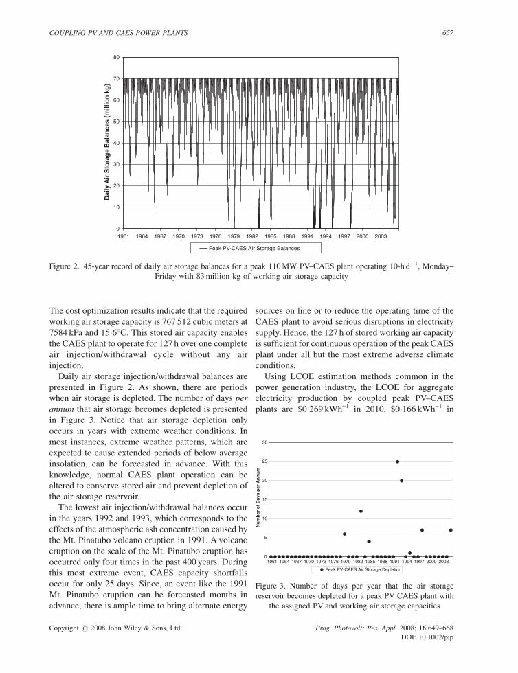
Figure 2. 45-year record of daily air storage balances for a peak 110 MW PV–CAES plant operating 10-h d�1, Monday–

Friday with 83 million kg of working air storage capacity

0

5

10

15

20

25

30

1961 1964 1967 1970 1973 1976 1979 1982 1985 1988 1991 1994 1997 2000 2003

Nu

mb

er o

f D

ays

per

An

nu

m

Peak PV-CAES Air Storage Depletion

Figure 3. Number of days per year that the air storage

reservoir becomes depleted for a peak PV CAES plant with

the assigned PV and working air storage capacities


The cost optimization results indicate that the required

working air storage capacity is 767 512 cubic meters at

7584 kPa and 15�68C. This stored air capacity enables

the CAES plant to operate for 127 h over one complete

air injection/withdrawal cycle without any air

injection.

Daily air storage injection/withdrawal balances are

presented in Figure 2. As shown, there are periods

when air storage is depleted. The number of days per

annum that air storage becomes depleted is presented

in Figure 3. Notice that air storage depletion only

occurs in years with extreme weather conditions. In

most instances, extreme weather patterns, which are

expected to cause extended periods of below average

insolation, can be forecasted in advance. With this

knowledge, normal CAES plant operation can be

altered to conserve stored air and prevent depletion of

the air storage reservoir.

The lowest air injection/withdrawal balances occur

in the years 1992 and 1993, which corresponds to the

effects of the atmospheric ash concentration caused by

the Mt. Pinatubo volcano eruption in 1991. A volcano

eruption on the scale of the Mt. Pinatubo eruption has

occurred only four times in the past 400 years. During

this most extreme event, CAES capacity shortfalls

occur for only 25 days. Since, an event like the 1991

Mt. Pinatubo eruption can be forecasted months in

advance, there is ample time to bring alternate energy


sources on line or to reduce the operating time of the

CAES plant to avoid serious disruptions in electricity

supply. Hence, the 127 h of stored working air capacity

is sufficient for continuous operation of the peak CAES

plant under all but the most extreme adverse climate

conditions.

Using LCOE estimation methods common in the

power generation industry, the LCOE for aggregate

electricity production by coupled peak PV–CAES

plants are $0�269 kWh–1 in 2010, $0�166 kWh–1 in


DOI: 10.1002/pip

Figure 4. Cost of electricity comparison between PV only, peak PV CAES plants, peak conventional GT plants, and peak

NGCC plants with CCS. The assumed fuel price for natural gas is $6 GJ�1, which is the approximate contract natural gas

price for electric utilities in the US in 2006, which is the last year for reported information. However, contract natural gas

price for electric generating companies has risen above $6 GJ�1, which means that the fuel price sensitivity findings

presented in Figure 6 are the best means to compare cost of electricity

658 J. MASON ET AL.

2015, and $0�135 kWh–1 in 2020 (refer to Figure 4).

The assumed fuel price is $6�0/GJ for natural gas.8 An

HVDC transmission cost of $0�024 kWh–1 is included

in the PV–CAES cost of electricity estimates. An

average transmission between PV and CAES plants of

2400 km is assumed with 7% electricity losses, which

includes the 1% loss incurred at the DC–AC converter

station. The CO2 emissions rate for PV–CAES plants is

97 g CO2 kWh–1, which includes the contributions

from the combustion of natural gas and from the life-

cycle of CO2 emissions for the PV electricity35,36.

The electricity cost estimates presented in this study

are derived through the net present value cash flow

method with the financial assumptions presented in

Table II. The financial assumptions are based on EPRI–

DOE37 with downward insurance and property tax

adjustments for PV power plants located in the remote

Southwest US.9 We are not attempting to derive

8The natural gas price of $6 GJ�1 is lower than the average 2007 and2008 contract natural gas price for US electricity generators.9The Southwest US land area suitable for PV plants is undeveloped,hence low property taxes. Also, approximately 50% of the costs forPV plant components do not qualify for insurance since they havezero risk for loss, for example mounting supports, undergroundconduit, land, etc.34


definitive cost of electricity estimates since estimates

are sensitive to variation in financial assumptions. On a

final note, financial incentives such as investment tax

credits and the effects of potential carbon taxes are not

included in the cost of electricity estimates.

Sensitivity analyses are performed to evaluate the

effect of changes in fuel cost, PV and CAES plant

capital costs, and HVDC transmission distance on PV–

CAES cost of electricity. The effect of fuel cost on PV–

CAES cost of electricity is presented in Figure 6. A $1/

GJ change in fuel cost changes the cost of electricity

by $0�0015 kWh–1. The small sensitivity of cost of

electricity to changes in fuel cost is attributable to the

small amount of natural gas consumed by coupled PV–

CAES power plants. The sensitivity of the cost of

electricity to changes in the other factors is presented

in Figure 7. A $100 kW–1 change in PV and CAES

plant capital costs changes the cost of electricity by

$0�004 and $0�003 kWh–1, respectively, and a change

in HVDC transmission distance of 500 km changes the

cost of electricity by $0�005 kWh–1.

We now turn our attention to a comparison of cost of

electricity for 2020 peak PV–CAES plants to those for

conventional peak GT power plants and NGCC power

plants. The cost of electricity comparison is presented


DOI: 10.1002/pip


in Figure 4. The cost of electricity estimate is

$0�108 kWh–1 for conventional peak GT plants and

$0�101 kWh–1 for peak NGCC plants. Notice in

Figure 6 the greater sensitivity of GT and NGCC cost

of electricity to changes in fuel cost due to the greater

fuel consumption rate of peak GT and NGCC plants

compared to peak PV–CAES plants. While the

comparative cost of electricity findings indicate that

at relatively low natural gas prices peak GT and

NGCC power plants produce lower cost electricity

than peak PV–CAES plants, the recent upward trend

in natural gas prices suggests that by 2020 peak

PV–CAES plants may become a cost competitive

source of peak electricity supply without any economic

recognition of the value of their carbon dioxide

reduction.

The CO2 emissions rate for conventional GT plants

is 553 g CO2 kWh–1,35 which is seven times greater

than the aggregate CO2 emissions rate for PV–CAES

peak plants. Comparative power plant CO2 emissions

rates are presented in Figure 5. The installation of CCS

systems at peak GT plants results in a significant

increase in the cost of electricity and because of this

has not been included in the analysis. On the other

hand, NGCC plants with CCS systems produce low

cost electricity and produce less CO2 emissions than

does a coupled PV–CAES plant. There is no indication

that peak electricity production by coal power plants

with CCS systems is cost competitive since the costs of

Figure 5. Power plant carbon dioxide emissio


coal power plants are much greater than GT plants, and

coal steam turbine plants do not have fast ramp-up and

ramp-down capabilities.

The capital cost of a 2020 peak PV–CAES plant is

$2749 kW–1, which is a factor of 5�7 greater than the

$485 kW–1 capital cost of a conventional peak GT

plant and a factor of 2�3 greater than the $1172 kW–1

capital cost of a peak NGCC plant with CCS. However,

annual fuel and O&M expenses are greater for peak GT

and NGCC plants compared to peak PV–CAES plants.

Notice in Figure 6 that when fuel cost exceeds $8�5/GJ

that the cost of electricity for peak PV–CAES plants is

lower than that for peak GT plants and when fuel cost

exceeds $10�2/GJ that the cost of electricity for peak

PV–CAES plants is lower than that for peak NGCC

plants with CCS.

Even the 2015 PV–CAES numbers can compare

favorably with conventional generators if the price of

fuel reaches the high end of the sensitivity domain

given in Figure 6. The effect of high fuel cost on

annualized cash flows can offset the capital cost

differential between peak PV–CAES power plants and

peak GT and NGCC with CCS power plants. Since the

course of fuel prices is largely unpredictable, it is

possible that PV–CAES may become cost-competitive

well prior to 2020. Another factor that is not accounted

in our comparison are the safety risks related to

transportation and storage of CO2, a heavier than air

asphyxiant gas.38

ns per kilowatt-hour of electricity produced


DOI: 10.1002/pip

0.08

0.10

0.12

0.14

0.16

0.18

0.20

0.22

$6 $7 $8 $9 $10 $11 $12

Fuel Cost ($/GJ)

Co

st o

f E

lect

rici

ty (

$/kW

h)

Peak PV CAES LCOE Sensitivity to Fuel Cost

Peak GT LCOE Sensitivity to Fuel Cost

Peak NGCC w/CCS LCOE Sensitivity to Fuel Cost

Figure 6. Sensitivity of peak PV–CAES, conventional GT, and NGCC power plants LCOE to changes in fuel cost. The

modeled power plants operate on average 10 h day�1, Monday–Friday, which is a 30% capacity factor

660 J. MASON ET AL.

The final issue to be considered in the analysis of

peak PV–CAES plants is the economic justification of

HVDC distribution of Southwest PV electricity to

CAES plants distributed outside the Southwest. As

0.110

0.115

0.120

0.125

0.130

0.135

0.140

0.145

0.150

0.155

0.160

-3 -2 -1Low Va

Co

st o

f E

lect

rici

ty (

$/kW

h)

Sensitivity to Change in CAES Plant Cap

Sensitivity to Change in PV Plant Capita

Sensitivity to Change in HVDC Transmis

Figure 7. Sensitivity of peak PV–CAES LCOE to changes i

transmissio


noted in the sensitivity findings, the impact of HVDC

cost on peak PV–CAES cost of electricity is

approximately $0�005 kWh–1 per 500 km of trans-

mission distance. The impact of reduced insolation on

3210lue to High Value

ital Costs (per $100/kW - Mean $877/kW)

l Costs (per $100/kW - Mean $1,300/kW)

sion Distance (per 500 km - Mean 2,400 km)

n CAES plant capital costs, PV plant costs, and to HVDC

n distance


DOI: 10.1002/pip


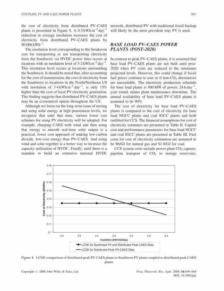
the cost of electricity from distributed PV–CAES

plants is presented in Figure 8. A 0�5 kWh m–2 day–1

reduction in average insolation increases the cost of

electricity from distributed PV–CAES plants by

$0�006 kWh–1.

The insolation level corresponding to the breakeven

cost for transporting or not transporting electricity

from the Southwest via HVDC power lines occurs at

locations with an insolation level of 5�2 kWh m–2 day–1.

This insolation level occurs at locations surrounding

the Southwest. It should be noted that, after accounting

for the cost of transmission, the cost of electricity from

the Southwest to locations in the North/Northeast US

with insolation of 3�4 kWh m–2 day–1, is only 15%

higher than the cost of local PV electricity generation.

This finding suggests that distributed PV–CAES plants

may be an economical option throughout the US.

Although we focus on the long-term issue of storing

and using solar energy at high penetration levels, we

recognize that until that time, various lower cost

schemes for using PV electricity will be adopted. For

example, charging CAES with wind and then using

that energy to smooth real-time solar output is a

practical, lower cost approach of making low-carbon

dioxide, low-cost energy than PV–CAES. And using

wind and solar together is a better way to increase the

capacity utilization of HVDC. Finally, until there is a

mandate to build an extensive national HVDC

0.1

0.11

0.12

0.13

0.14

0.15

0.16

0.17

0.18

3.4 3.9 4.4

Insolatio

Co

st o

f E

lect

rici

ty (

$/kW

h)

LCOE for Southwest P

LCOE for Distributed P

Figure 8. LCOE comparison of distributed peak PV CAES pla

plan


network, distributed PV with traditional fossil backup

will likely be the most prevalent way PV is used.

BASE LOAD PV–CAES POWERPLANTS (POST-2020)

In contrast to peak PV–CAES plants, it is assumed that

base load PV–CAES plants are not built until post-

2020 when PV costs are reduced to the minimum

projected levels. However, this could change if fossil

fuel prices continue to soar or if non-CO2 alternatives

are unavailable. The electricity production schedule

for base load plants is 400 MW of power, 24 h day–1,

year round, minus plant maintenance downtime. The

annual availability of base load PV–CAES plants is

assumed to be 90%.

The cost of electricity for base load PV–CAES

plants is compared to the cost of electricity for base

load NGCC plants and coal IGCC plants and both

outfitted for CCS. The financial assumptions for cost of

electricity estimates are presented in Table II. Capital

cost and performance parameters for base load NGCC

and coal IGCC plants are presented in Table III. Fuel

costs for cost of electricity estimation are assumed to

be $6/GJ for natural gas and $1�8/GJ for coal.

CCS system costs include power plant CO2 capture,

pipeline transport of CO2 to storage reservoirs,

4.9 5.4 5.9 6.4

n (kWh/m2/day)

V and Distributed Peak CAES Sites

eak PV-CAES Sites

nts to Southwest PV plants coupled to distributed peak CAES

ts


DOI: 10.1002/pip

Table III. Fossil fuel power plant cost and performance parameters39�

A. Natural gas CC with CCS

Total plant costs ($ kW�1) 1172 39

Plant capacity factor 0�85 39

Fixed O&M ($ kW�1) 16�637 39

Variable O&M ($ kWh�1) 0�0026 39

Heat rate (MJ kWh�1) 8�237 39

Parasitic power loss (% Of power output) 7% 39

GHG emissions (g CO2 kWh�1) 42 39

B. Coal IGCC with CCS

Total plant costs ($ kW�1) 2496 39

Plant capacity factor 0�8 39

Fixed O&M ($ kW�1) 44�586 39

Variable O&M ($ kWh�1) 0�0082 39

Heat rate (MJ kWh�1) 11�227 39

Parasitic power loss (% of Power output) 25% 39

GHG emissions (g CO2 kWh�1) 100 39�Heat rates are reported at the high heat value.

662 J. MASON ET AL.

reservoir development, and long-term reservoir

monitoring. Cost estimates for CO2 transport, storage,

and monitoring are reported to be $0�004 kWh–1.39

However, these estimates are based on very optimistic

conditions, a CO2 transport distance of only 80 km and

compressors at only the point of CO2 production, and

therefore may not be representative of true CO2

transport costs. The results of a sensitivity analysis

indicate that the cost of electricity sensitivity to a

$100 kW–1 change in CCS costs is $0�001 kWh–1 for

NGCC and coal IGCC power plants.

For base load PV–CAES plants, the PV electricity

production profile created from the 45-year NSRDB

insolation record indicates that a 1�613 GW PV power

plant will support a 400 MW base load CAES power

plant. The electricity output from 507 MW of the total

PV capacity is dedicated to grid distribution, and the

electricity output from the remaining 1106 MW of PV

capacity is consigned to the CAES plant for air

compression. This allocation of PV electricity occurs

7 days a week, year-round.

The volume of the air storage reservoir for the base

load CAES plant is 6�88 million cubic meters of

working air capacity at 7584 kPa and 15�68C. This

quantity of stored compressed air is able to maintain

312 h of CAES plant operation without any air

injection. Daily air storage balances are presented in

Figure 9, and the number of days per annum that air

storage is depleted is presented in Figure 10. Just as in

the peak PV–CAES scenario, the time of year with

lowest air storage balances is the low insolation late-


fall and winter months. Hence, plant maintenance

downtime should be scheduled in late-fall and early

winter to recharge and conserve air storage capacity.

On the other hand, compressor maintenance downtime

should be scheduled in the high insolation spring

period when reservoir recharging is relatively rapid.

Also, notice in Figure 10 that the years when air

storage depletion occurs are those years experiencing

extreme low insolation climate conditions such as the

years following the 1991 Mt. Pinatubo volcano

eruption with the maximum air storage depletion of

29 days. As stated previously, these low insolation

climate conditions can be forecast in advance and

CAES plant operating schedule adjusted to conserve

air storage capacity.

With the base load PV–CAES model adopted for this

study, PV plants directly produce 36% of aggregate PV–

CAES electricity production, and the CAES plant

produces the remaining 64%. The average daily CAES

operating factor is 72%. In 2020, the aggregate cost of

electricity estimate for base load PV–CAES plants is

$0�118 kWh–1. The PV–CAES cost of electricity estimate

includes $0�024 kWh–1 to transport electricity via HVDC

power lines from the Southwest PV plants to distributed

CAES plants at an average distance of 2400 km and with

7% electricity losses. The aggregate CO2 emissions rate

is 164 g CO2 kWh–1, which includes the CAES plant

contribution from the combustion of natural gas and the

life-cycle CO2 emissions for PV electricity.35,36

The capital costs for a 400 MW-base load CAES

plant with a supporting 1�613 GW PV plant are


DOI: 10.1002/pip

0

100

200

300

400

500

600

700

1961 1964 1967 1970 1973 1976 1979 1982 1985 1988 1991 1994 1997 2000 2003

Dai

ly A

ir S

tora

ge

Bal

ance

s (m

illio

n k

g)

Base Load PV-CAES Air Storage Balances

Figure 9. 45-year record of daily air storage balances for a base load PV–CAES plant. The operating schedule includes

36 days of turbo-generator set downtime for normal maintenance scheduled from December 1 to January 6 each year, and

10 days of compressor downtown for normal maintenance scheduled from April 21–April 30 each year


$6681 kW–1. In contrast, the capital costs for 400 MW

NGCC and coal IGCC plants with CCS are $1172 and

$2496 kW–1, respectively.39 The cost of electricity

estimate for base load PV–CAES plants is

0

5

10

15

20

25

30

35

1961 1964 1967 1970 1973 1976 1979 19

Nu

mb

er o

f D

ays

per

An

nu

m

Baseload PV-CAE

Figure 10. Number of days per year that the air storage reservo

assigned PV and workin


$0�118 kWh–1. The base load PV–CAES cost of

electricity estimate is compared to the cost of

electricity estimates for the base load NGCC and coal

IGCC plants, and the findings are presented in

82 1985 1988 1991 1994 1997 2000 2003

S Air Storage Depletion

ir becomes depleted for a base load PV CAES plant with the

g air storage capacities


DOI: 10.1002/pip

Figure 11. Cost of electricity estimates for base load PV–CAES (2020 PV model) and base load Natural Gas CC and Coal

IGCC power plants with CCS. Assumed fuel prices: natural gas¼ $6 GJ�1; coal¼ $1�8 GJ�1

664 J. MASON ET AL.

Figure 11. The reported electricity cost estimate for

base load NGCC plants is $0�076 kWh–1, and the

estimate for base load coal IGCC plants is

$0�087 kWh–1, which are 36% and 26% lower than

the cost of electricity for base load PV–CAES plants,

respectively.

0.06

0.07

0.08

0.09

0.10

0.11

0.12

0.13

0.14

0.15

0.16

0.17

0% 25% 50%

% Increase in Fuel Cost (In

Co

st o

f E

lect

rici

ty (

$/kW

h)

Baseload PV CAES Baseload NGCC

Figure 12. Sensitivity of cost of electricity to increases in fuel

IGCC power pla


The sensitivity of cost of electricity for the base load

power plants to change in fuel cost is presented in

Figure 12. As expected, the cost of electricity from

NGCC plants is the most sensitive to change in fuel

cost. The breakeven cost of electricity for base load

PV–CAES and NGCC plants with CCS is $0�141 kWh–1

75% 100% 125% 150%

itial Cost: NG $6/GJ; Coal $1.80/GJ)

with CCS Baseload Coal IGCC with CCS

cost for base load PV–CAES plants, NGCC plants, and coal

nts with CCS


DOI: 10.1002/pip

0.09

0.10

0.11

0.12

0.13

0.14

0.15

0.16

0.17

3.4 3.9 4.4 4.9 5.4 5.9 6.4

Insolation (kWh/m2/day)

Co

st o

f E

lect

rici

ty (

$/kW

h)

LCOE for Southwest PV and Distributed Base Load CAES Sites

LCOE for Distributed Base Load PV-CAES Sites

Figure 13. LCOE comparison of distributed base load PV CAES plants to Southwest PV plants coupled to distributed base

load CAES plants


and occurs with a fuel cost of $13�5 GJ–1, which is

125% greater than the $6 GJ–1 baseline fuel cost.

The determination of the breakeven cost of

electricity between 2020-modeled PV–CAES and coal

IGCC plants is problematic since two fuels are

involved. Based on the cost of electricity trajectories

for base load PV–CAES and coal IGCC plants

presented in Figure 12, it is unlikely that the fuel

cost mix will result in base load PV–CAES as an

economically viable option in 2020. In addition, it

should be noted that the base load PV–CAES cost of

electricity estimates are significantly greater than the

cost of electricity estimates for base load wind-CAES

plants.7,8

As with the peak PV–CAES scenario, an analysis of

distributed base load PV–CAES plants is performed,

and the cost of electricity estimates compared to those

for the model with PV electricity generated in the

Southwest and transmitted via HVDC to CAES plants

distributed across the country. The comparison is

presented in Figure 13. The cost of electricity

breakeven point occurs at locations with an average

insolation level of 5�9 kWh m–2 day–1, which is

substantially greater than the peak PV–CAES finding.

Locations with an average insolation level of

5�9 kWh m–2 day–1 can only be found in the Southwest.

But once again, the impact on cost of electricity is

relatively small, 22% greater than that at worst case


insolation locations, which implies that distributed

base load PV–CAES plants may be an economically

feasible option.

CONCLUSION

A summary of the findings for the 2020-modeled peak

and base load PV–CAES plants is as follows. The

aggregate LCOE for peak PV–CAES plants is

$0�135 kWh–1, and for base load PV–CAES plants it

is $0�118 kWh–1. The aggregate fuel consumption for

peak PV–CAES plants is 2�0 MJ kWh–1, and for base

load PV–CAES plants it is 3�55 MJ kWh–1. The

aggregate CO2 emissions rate for peak PV–CAES

plants is 97 g CO2 kWh–1, and for base load PV–CAES

plants it is 164 g CO2 kWh–1.

And important finding is that by 2020 peak PV–

CAES plants might be cost competitive with peak

electricity production by conventional GT power

plants and by NGCC with carbon and capture systems

power plants. On the other hand, our findings suggest

that the cost of electricity for base load PV–CAES

plants will not be cost competitive with other sources

of base load electricity supply in 2020, unless fuel

prices increase dramatically from current levels.

While the capital cost of coupled peak PV–CAES

plants is a factor of two or more greater than the capital


DOI: 10.1002/pip

666 J. MASON ET AL.

cost of comparable fossil fuel peak power plants, the

low heat rate of peak PV–CAES plants moderates the

effect of fuel costs on annualized cash flows, and

significantly improves the economic viability of peak

PV–CAES plants. Such effect would be even greater,

if, as expected near-adiabatic CAES plants are

developed by 2020.

Our peak PV–CAES findings are important since

there is a relatively good chance that natural gas prices

in 2020 will be at a high enough level to make peak

PV–CAES electricity production cost competitive. The

natural gas cost level where the cost of electricity for

peak PV–CAES plants is equal to the cost of electricity

for conventional peak GT plants without CCS systems

is $8�5 GJ–1 and for NGCC power plants with CCS it is

$10�2 GJ–1. These natural gas prices are not that much

higher than the 2007 electric utility contract price for

natural gas. Indeed, if natural gas prices take a

continued rising path, we may have to revisit the

economics of the 2015 peak PV–CAES model.

The low heat rate of peak PV–CAES plants is

conducive for the utilization of bio-syngas, which if

used by PV–CAES plants will result in a near-zero CO2

emissions path. With a bio-syngas cost of $13 GJ–1, the

2020 cost of electricity for a peak PV–CAES plant is

$0�146 kWh–1, which is cost competitive with peak GT

power plants at a natural gas cost of $9�0 GJ–1 and with

NGCC plants with CCS systems at a natural gas cost of

$10�5 GJ–1.

To distribute PV electricity produced in the South-

west to local markets throughout the country will

require the construction of a national HVDC power

distribution system. To distribute the electricity from a

PV power plant capacity of one terawatt will require

the construction of 200 5-GW HVDC lines. While this

will require extensive planning, it is considered doable

based on current planning for extensive HVDC

systems in China and India. And the cost is not

prohibitive since it increases the cost of electricity

produced by PV–CAES plants at an average 2400 km

transmission distance by only $0�024 kWh–1.

An alternative to a national HVDC system to

distribute Southwest PV electricity is distributed PV

plants located throughout the country and in close

proximity to distributed CAES plants. While the cost

of electricity by distributed PV power plants is greater

than the Southwest PV model, the net increase in cost

of electricity at the lowest US insolation site is just

15%. Therefore, distributed PV–CAES plants may

prove economically viable. However, it should be

noted that factors other than insolation may increase


the cost of distributed PV–CAES plants relative to

Southwest PV plants and distributed CAES plants such

as a need for costly concrete mounting foundations to

protect against tornado activity, high land costs, and

increased fuel consumption by the CAES plant in

response to greater diurnal variability in insolation. In

conclusion, distributed PV–CAES plants require

greater depth of analysis than provided in this study

before a firm conclusion can be reached.

We do not consider numerous other possible short,

mid-, and long-term combinations of PV, CAES,

HVDC, wind, other renewables, and conventional

backup. These deserve further study as they may

represent practical paths in terms of economics and

carbon dioxide avoidance.

On a final note, the operating life of PV modules is

longer than 30 years and may exceed 60 years. In

addition, the operating life of PV balance of plant

components, i.e., PV mounting supports and under-

ground wiring conduits, is at least 60 years in the arid

environment of the Southwest. Therefore, the

reduction in cost of electricity accruing from

amortization of power plants would be more favorable

for PV–CAES plants than aging fossil fuel plants. This

means a large post-amortization decrease in electricity

prices from PV–CAES plants, which translates into an

economically attractive long-term electricity price

trajectory for PV–CAES power plants.

REFERENCES

1. Zaugg P. Air-storage power generating plants. Brown

Boveri Review 1975; 62: 338–347.

2. Cavallo AJ. High-capacity factor wind energy systems.

Journal of SolarEnergy Engineering, Transactions of the

ASME 1995; 117: 137–143.

3. Denholm P, Kulcinski GL, Holloway T. Emissions and

energy efficiency assessment of baseload wind energy

systems’’. Environmental Science and Technology 2005;

39: 1903–1911.

4. Desai N, Gonzalez S, Pemberton DJ, Rathjen TW. The

Economic Impact of CAES on Wind in TX, OK, and

NM. Ridge Energy Storage & Grid Services L.P., Texas

State Energy Conservation Office June 27 2005.

5. Denholm P. Improving the technical, environmental

and social performance of wind energy systems using

biomass-based energy storage. Renewable Energy 2006;

31(2006): 1355–1370.

6. Cavallo A. Controllable and affordable utility-scale

electricity from intermittent wind resources and com-

pressed air energy storage (CAES). Energy 2007; 32:

120–127.


DOI: 10.1002/pip


7. Greenblatt JB, Succar S, Denkenberger DC, Williams

RH, Socolow RH. Base load wind energy: modeling the

competition between gas turbines and compressed air

energy storage for supplemental generation. Energy

Policy 2007; 35: 1474–1492.

8. Succar S., Williams RH. Compressed Air Energy Sto-

rage: Theory, Resources, and Applications for Wind

Power. Report prepared by the Energy Systems Analysis

Group, Princeton Environmental Institute, Princeton

University 2008.

9. Fthenakis Vasilis, James M, Mason E, Ken Zweibel. The

technical, geographical and economic feasibility for

solar energy to supply the energy needs of the United

States. Energy Policy, In press.

10. Mason JE, Fthenakis VM, Hansen T, Kim HC. Energy

payback and life-cycle [2co] emissions of the bos in an

optimized 3.5-mw pv installation. Progress in Photo-

voltaics: Research and Applications 2006; 14(2): 179–

190.

11. DeCorso Richard, Lee Davis, Dennis Horazak, John

Molinda, Mario DeCorso. Parametric study of payoff

in applications of air energy storage (CAES) plants – an

economic model for future applications.’’ Paper pre-

sented at Power Gen International Conference, Orlando,

Florida, November 2006.

12. NREL. National Solar Radiation Data Base, 1961–

1990. Renewable Resource Data Center, National

Renewable Energy Laboratory (NREL), Golden, CO.

http://rredc.nrel.gov/solar/old_data/nsrdb 2007a.

13. NREL. National Solar Radiation Data Base, 1991–

2005. Renewable Resource Data Center, National

Renewable Energy Laboratory (NREL), Golden, CO.

http://rredc.nrel.gov/solar/old_data/nsrdb 2007b.

14. Marion W, Wilcox S. Solar Radiation Data Manual for

Flat-Plate and Concentrating Collectors. Manual Pro-

duced by the National Renewable Energy Laboratory’s

Analytic Studies Division. Contract No. NREL/TP-463-

5607, DE93018229, April 1994.

15. Falck L. Personal communication with Lars Falck of the

JUWI Group 2008.

16. Hansen TN. The promise of utility scale solar photovoltaic

(pv) distributed generation. Presented at POWER-GEN

International, Las Vegas, NV, 10 December 2003.

17. Juwi. 2007, Press release ‘‘World’s largest solar power

plant being built in eastern Germany.’’ http://www.juwi.

de/international/information/press/PR_Solar_Power_

Plant_Brandis_2007_02_eng.pdf

18. Lesser J, Puga N. PV vs. solar thermal. Public Utilities

Fortnightly July 2008: 2008, 17–20, 27.

19. Zweibel K. The terawatt challenge for thin film pv. In

Thin Film Solar Cells: Fabrication, Characterization

and Applications. Poortmans J, Archipov V (eds). Bos-

ton, John Wiley, 2005 1396–1408.

20. Keshner MS, Arya R. 2004; Study of Potential Cost

Reductions Resulting from Super-Large-Scale Manufac-


turing of PV Modules. Final Subcontract Report, NREL/

SR-520-36846, October (2004), National Renewable

Energy Laboratory, US Department of Energy, Golden,

CO. http//:www.nrel.gov/docs/fy05osti/36846.pdf

21. Ginley D, Green M, Collins R. Solar energy conversion

toward 1 terawatt. MRS Bulletin 2008; 33(4): 355–364.

22. DLR. Trans-Mediterranean Interconnection for Concen-

trating Solar Power. German Aerospace Center (DLR),

Institute of Technical Thermodynamics, Section Sys-

tems Analysis and Technology Assessment. Federal

Ministry for the Environment, Nature Conservation

and Nuclear Safety, Stuttgart, Germany 2006.

23. de Andres J., Miques Perez, Miguel Muhlenkamp, Diet-

mar Retzmann, Roland Walz. Prospects for HVDC:

getting more power out of the grid. Presentation prepared

for Siemens AG and presented at the CIGRE Confer-

ence, Madrid, Spain, 29–30 November 2006.

24. Dorn Joerg, Dietmar Retzmann, Cristen Schimpf, Dag

Soerangr. HVDC solutions for system interconnection

and advanced grid access. Presentation for Siemens AG

at the EPRI HVDC Conference, 13–14 September 2007.

25. McCoy Paul, Vaninetti Jerry. It’s doable: building trans-

mission for solar. EnergyBiz 2008; 5(2): 40.

26. Mehta B. 1992, CAES geology. EPRI J 1992 (October/

November): 38–41.

27. AGA. Examining Natural Gas Storage for Local Distri-

bution Companies. Final report prepared by Inter-

national Gas Consulting, Inc., Houston, TX for the

American Gas Association (AGA), Washington, DC,

May 1998.

28. Davis L., Schainker BR. Compressed Air Energy Storage

(CAES): Alabama Electric Cooperative McIntosh Plant –

Overview and Operational History. Report prepared

jointly by the Alabama Electric Cooperative and the

Electric Power Research Institute (EPRI). EPRI; Palo

Alto, CA 2006.

29. Schwartz J. The gas compression formula was given to

Mason by Joseph Schwartz, a gas dynamics engineering

specialist with Praxair 2005.

30. Peress J. Working with non-ideal gases: here are two

proven methods for predicting gas compressibility fac-

tors. CEP Magazine 2003; 39–41.

31. Bullough C., Gatzen C, Jakiel C, Koller M, Nowi A, Zunft

S. Advanced adiabatic compressed air energy storage for

the Integration of wind energy. Presented at the Proceed-

ings of the European Wind Energy Conference, EWEC

2004, 22–25 November 2004, London UK.

32. Zunft S., Christoph J, Martin K, Chris B. Adiabatic

compressed air energy storage for the grid integration

of wind power. Presented at the Sixth International

Workshop on Large-Scale Integration of Wind Power

and Transmission Networks for Offshore Windfarms, 26–

28 October 2006, Delft, The Netherlands 2006.

33. Swensen E, Potashnik B. Evaluation of Benefits and

Identification of Sites for a CAES Plant in New York


DOI: 10.1002/pip

668 J. MASON ET AL.

State. Report prepared by Energy Storage and Power

Consultants in association with ANR Storage Company

for Electric Power Research Institute (EPRI). TR-

104288, Research Project, Final Report, August 1994,

EPRI, Palo Alto, CA 1994.

34. EIA. Annual Energy Outlook Energy Information

Administration (EIA), DOE/EIA-0554 (2007), US

Department of Energy, Washington, DC, March

2007.

35. Wang M. GREET Version 1.7 (Excel Interactive Version).

Center for Transportation Research, Argonne National

Laboratory, University of Chicago, Chicago, IL 2001.

36. Fthenakis V, Hyung M, Chul K. Greenhouse-gas emis-

sions from solar electric- and nuclear power: a life cycle

study. Energy Policy 2007; 35(4): 2540–2557.


37. EPRI-DOE. EPRI-DOE Handbook of Energy Storage for

Transmission and Distribution Applications. Report Number

1001834, Electric Power Research Institute (EPRI), Palo Alto,

CA and the US Department of Energy, Washington, DC 2003.

38. Elgin B. The dirty truth about clean coal. Business Week

June 2008; 30: 55–56.

39. NETL. Cost and Performance Baseline for Fossil Energy

Plants, Vol. 1. Report DOE/NETL-2007/1281, National

Energy Technology Laboratory (NETL): Washington, DC,

May 2007.

40. Zweibel K, James EM, Vasilis F. A solar grand plan.

Scientific American 2008; 298(1): 64–73.

41. Copeland TE, Weston JF. Financial Theory and Cor-

porate Policy, 3rd Ed. Addison-Wesley Publishing Com-

pany: Reading, MA, USA 1992.


DOI: 10.1002/pip

Documents

Research Coupling PV and CAES Power Plants to Transform ... · Plants to Transform Intermittent PV Electricity into a Dispatchable ... combined-cycle ... PV mounting supports, grounding