Residential Rent Affordability across U.S. Metropolitan Areas

Kelly D. Edmiston Federal Reserve Bank of Kansas City

Working Paper 17-20

June 2017

The views expressed herein are those of the authors and not necessarily those of the Federal Reserve Bank of Minneapolis or the Federal Reserve System. This paper was originally published as Economic Review, Fourth Quarter 2016 by the Federal Reserve Bank of Kansas City. This paper may be revised. The most current version is available at https://www.kansascityfed.org/~/media/files/publicat/econrev/econrevarchive/2016/4q16edmiston.pdf. __________________________________________________________________________________________

Opportunity and Inclusive Growth Institute Federal Reserve Bank of Minneapolis • 90 Hennepin Avenue • Minneapolis, MN 55480-0291

https://www.minneapolisfed.org/institute

Owner-occupied housing has become more affordable in most markets since the housing crisis (National Association of Re-altors Housing Affordability Index). But many renters and

their advocates have reported that rental housing has become increas-ingly unaffordable. Median residential rent rose at an annual rate of 2.3 percent nationally from 2010 to 2015, according to the American Community Survey (ACS). When adjusted for inflation—which rose 1.7 percent as measured by the compound annual rate of change in the Consumer Price Index—annual median rent grew by 0.6 percent.

While rents have been rising moderately faster than inflation, they do not necessarily indicate declining affordability. Rather, rental hous-ing becomes less affordable when rent increases relative to income. By this measure, rental housing has indeed become less affordable at the national level. National personal income declined at an inflation-ad-justed annual rate of 0.4 percent from 2010 to 2015. Thus, rent growth outpaced income growth by 1 percentage point (0.6−[−0.4]) annually.

National data on rent affordability are useful for understanding macroeconomic conditions and policies, but they mask important de-tails about local markets. Specifically, affordability—and changes in af-fordability—vary widely across metropolitan statistical areas (MSAs).

Residential Rent Affordability across U.S. Metropolitan AreasBy Kelly D. Edmiston

Kelly D. Edmiston is a senior economist at the Federal Reserve Bank of Kansas City. Daniel Perez, a research associate at the bank, helped prepare the article.This article is on the bank’s website at www.KansasCityFed.org

5

6 FEDERAL RESERVE BANK OF KANSAS CITY

Properly addressing concerns around housing affordability requires identifying not only the areas with troubling affordability trends but also what makes these areas different from others.

The affordability of rental housing is an especially important con-cern for low- and moderate-income (LMI) households, which have incomes 80 percent or below MSA median income. LMI households have fewer resources to dedicate to housing and often find their housing circumstances to be tenuous. While middle-income households usually have more stable housing, they too are increasingly facing budget con-straints: in higher-cost areas in particular, middle-income households are devoting more of their resources to housing, leaving less for other essential expenditures and important long-term financial goals such as higher education and retirement.

In this article, I highlight patterns in rental housing affordability for both LMI and middle-income (specifically, median-income) house-holds. I first examine patterns across LMI households using the U.S. Department of Housing and Urban Development’s (HUD) Fair Mar-ket Rents. Fair Market Rents are well-suited for their intended pur-pose—setting payment standards for assisted housing programs—but are not ideal for the more extensive analysis in this article. I therefore use data on median income and median rent not only to analyze pat-terns in housing affordability across median-income households, but also to highlight the variation in housing affordability across MSAs and to identify the factors that explain this variation.

When examining variability in housing affordability across MSAs, I find that many of the MSAs that have seen the greatest changes in affordability over the last five years have relatively small populations and an institution or industry that in some sense dominates the area—for example, large military installations, colleges and universities, or energy-related industries.

Section I discusses why rental housing affordability is an important socioeconomic concern. Section II analyzes rental affordability for LMI households. Section III examines affordability for median households, using median rent and income to identify factors explaining variation in rental housing affordability across MSAs and changes in affordability over time.

ECONOMIC REVIEW • FOURTH QUARTER 2016 7

I. Why Is Rental Housing Affordability a Critical Concern?

Shelter is among the most basic human requirements and is neces-sary for survival. A significant number of people in the United States lack affordable housing, and, along with it, housing security. Individu-als are insecure in their housing when it is at least sporadically unavail-able or when they must frequently change their residence.

In the extreme, a lack of affordable housing can lead to home-lessness.1 Housing insecurity also arises from nontraditional housing arrangements such as “doubling up” with friends or family or “couch surfing” among the residences of multiple friends and family mem-bers. These types of living arrangements are manifestations of the same primary problem underlying homelessness, which is an imbalance be-tween income and housing costs (Honig and Filer). Frequent changes in residence, often due to eviction, also erode housing security (Des-mond and Kimbo).

Housing insecurity can lead to several other problems. Those with-out secure housing report significantly poorer well-being (Johnstone and others). While poor physical health is associated with poverty gen-erally, it is more pronounced in populations without secure housing (American Psychological Association). In addition, housing insecurity can restrict social networks and generate barriers to education and em-ployment (Skobba and Goetz; Long, Rio, and Rosen). The effects of housing insecurity on children are well-documented and include not only poor health and nutrition, but also developmental delays, psy-chological problems, and educational underachievement (Rafferty and Shinn; Bassuk, Rubin, and Lauriat; Newman and Holupka).

Housing not only meets a basic physiological need, it also accounts for a substantial share of most household budgets, trumping transpor-tation, food, and health care. In 2015, the shelter component of hous-ing expenditure (mortgage payment or rent) accounted for 19.2 per-cent of total consumer expenditures among U.S. households—25.8 percent among renters (U.S. Bureau of Labor Statistics, Consumer Expenditure Survey). When utilities and taxes are included, the hous-ing share of expenditure is significantly higher. Low-income house-holds face especially high housing expenditures as a share of spending. In 2014, households in the bottom third of the income distribution

8 FEDERAL RESERVE BANK OF KANSAS CITY

spent 40 percent of their income on housing and related expenses (Pew Charitable Trusts).

II. Rental Housing Affordability for LMI Households

At its root, affordability is housing cost relative to income. The most common way to measure housing affordability, especially when evaluating affordability for LMI households, is to assess the financial burden housing costs place on household budgets. In affordable hous-ing research and advocacy, the threshold for being cost-burdened is almost uniformly defined as 30 percent of gross household income. A household with housing costs (rent or mortgage plus utilities) ex-ceeding 30 percent of their gross income is thereby considered “cost-burdened,” while a household with housing costs exceeding 50 percent of their gross income is considered “severely cost-burdened.”

The 30 percent threshold is somewhat arbitrary, but it has a basis in the 1971 Brooke Amendment to the 1969 Housing Act, which capped public housing rents at 25 percent of income (in 1981, the threshold was raised to 30 percent). The Brooke Amendment was a response to rising rents, which led to widespread tenant discontent and a series of rent strikes in the 1960s.2

The most reliable data on rents available by MSA typically are aver-ages or medians, which are not well-suited for assessing rental housing affordability for LMI households. However, Fair Market Rents, which are set at the 40th percentile point within the distribution of market-rate rents, can provide a more useful measure.3 Fair Market Rents are calculated annually by HUD for use in setting payment standard amounts for the Housing Choice Voucher program. Because Fair Mar-ket Rent is set below median rent (by 10 percentage points), it better reflects the rents that lower-income households actually pay than medi-an or average rents. If renters were to select units in the same rank order as their incomes, households paying Fair Market Rent would be just on the cusp of the LMI threshold, or 80 percent of area median income.4

One way that Fair Market Rents can be used to evaluate rental housing affordability for LMI households is by constructing a “hous-ing wage” (see National Low Income Housing Coalition). The housing wage is the (gross) hourly full-time wage a renter would need to af-ford a standard quality unit at Fair Market Rent. The methodology for

ECONOMIC REVIEW • FOURTH QUARTER 2016 9

computing the housing wage begins by multiplying Fair Market Rent by 12 to get the annual rental cost and then dividing the annual rental cost by 0.3, the affordability threshold, to determine the total income needed to “afford” that rent. The required income is then converted to an hourly rate assuming a 40-hour workweek.

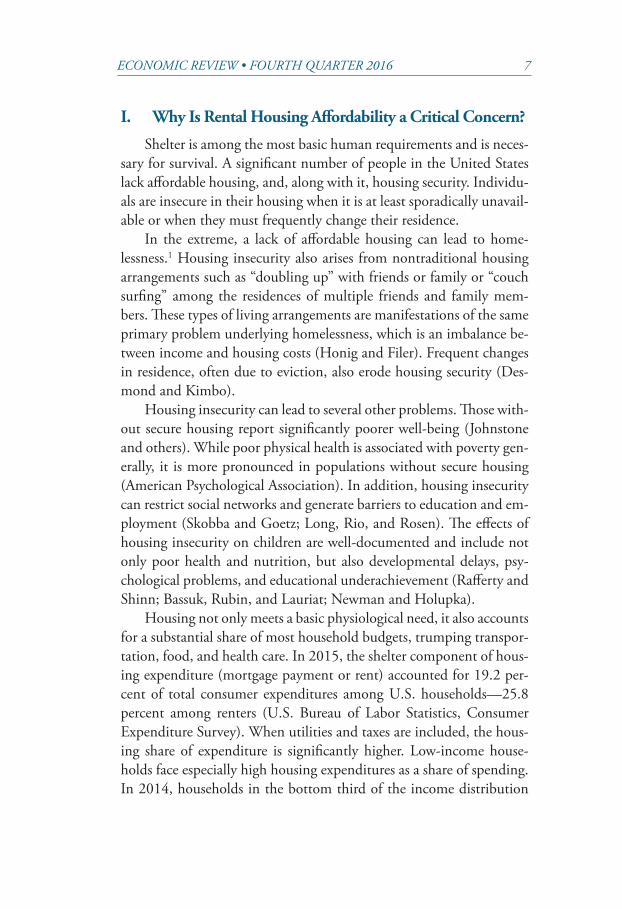
For the nation, the 2016 housing wage is $20.30 per hour. That is, a full-time worker in a single-earner household would need an hourly wage of $20.30 or more to rent a two-bedroom unit at Fair Market Rent without being cost-burdened. The national housing wage has in-creased only modestly over the last several years, growing at an annual rate of 2 percent from its value of $17.32 in 2008. By comparison, in-flation averaged 1.7 percent annually over that period. Housing wages vary substantially across MSAs (Chart 1). In 2016, the housing wage ranged from $11.90 in Florence-Muscle Shoals, AL, to $38.35 in San Jose, CA. The housing wage in Honolulu, HI, also was relatively high at $38.17. But both San Jose and Honolulu are outliers: the third high-est housing wage, in Washington, DC, was $31.21. By construction, the housing wage is proportional to the Fair Market Rent. A ranking of MSAs by housing wage is identical to a ranking by Fair Market Rent. In 2016, nine of the highest-cost MSAs for LMI households were in California. The exceptions were Washington, DC, New York, Boston, Seattle, and Barnstable Town, MA (which includes a number of resort communities such as Cape Cod).

To evaluate affordability, I compare the housing wage with earned wages. Specifically, I calculate the weekly hours of work at specific wage levels that would be required to rent a unit at Fair Market Rent without being housing-cost-burdened. Consider first workers earning the fed-eral minimum wage ($7.25 per hour as of December 2016) who live in single-earner households.5 Ignoring any statutory requirements for overtime pay, they would need to work 112 hours per week to afford a two-bedroom unit priced at Fair Market Rent ([$20.30 x 40]/$7.25). By comparison, workers at the 25th percentile of the wage distribution earned $11.27 per hour in 2016 (U.S. Bureau of Labor Statistics, Na-tional Compensation Survey). At that wage, they would need to work 72 hours to afford a unit at Fair Market Rent. Even at $15 per hour, which is currently being phased in as a minimum wage in some large cities, workers would need to work 54 hours per week to afford the

10 FEDERAL RESERVE BANK OF KANSAS CITY

national Fair Market Rent.6 Moreover, workers at the 50th percentile of the wage distribution ($21.94) would need to work nearly a full 40-hour week to afford a housing unit at the 40th percentile of the rent distribution—in other words, a housing unit at Fair Market Rent.7 This pattern has remained steady throughout the last several years, which suggests that those who have received typical wage increases over the last several years have not seen significant declines in affordability.

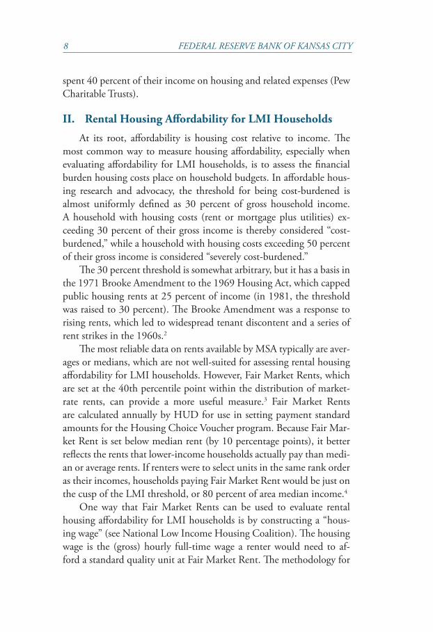
The housing wage also provides a useful framework for analyzing changes in affordability for LMI households over time. Chart 2 com-pares the change in housing wage from 2010 to 2016 to the 2010 hous-ing wage. The data show a clear negative relationship between the 2010 housing wage and the change in the housing wage over the following six years. That is, the MSAs with the highest housing wages in 2010 typi-cally saw the lowest percentage increase (or greatest decrease) in housing wage from 2010 to 2016, implying convergence in housing wages.

Market forces should lead some in high-cost areas to seek residence in lower-cost areas, which should decrease rents in the former and in-crease them in the latter. The data in Chart 2 are consistent with this expectation. Any convergence in housing wages likely would occur over a significant period of time. Moreover, a number of other factors also are important in determining rent growth. The data are scattered

Chart 12016 Housing Wage by MSA

Source: Author’s calculations using data from the U.S. Department of Housing and Urban Development (Fair Market Rents).

$5

$10

$15

$20

$25

$30

$35

$40

$45

$5

$10

$15

$20

$25

$30

$35

$40

$45

1 26 51 76 101 126 151 176 201 226 251 276 301 326 351

Housing wage Housing wage

MSAs

National housing wage: $20.30

ECONOMIC REVIEW • FOURTH QUARTER 2016 11

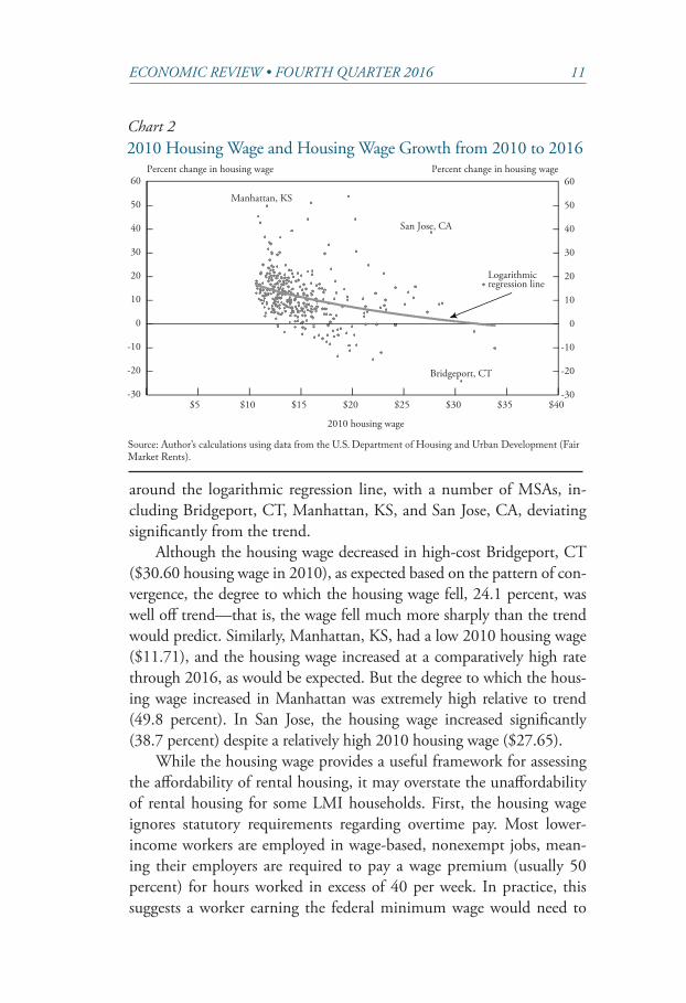
around the logarithmic regression line, with a number of MSAs, in-cluding Bridgeport, CT, Manhattan, KS, and San Jose, CA, deviating significantly from the trend.

Although the housing wage decreased in high-cost Bridgeport, CT ($30.60 housing wage in 2010), as expected based on the pattern of con-vergence, the degree to which the housing wage fell, 24.1 percent, was well off trend—that is, the wage fell much more sharply than the trend would predict. Similarly, Manhattan, KS, had a low 2010 housing wage ($11.71), and the housing wage increased at a comparatively high rate through 2016, as would be expected. But the degree to which the hous-ing wage increased in Manhattan was extremely high relative to trend (49.8 percent). In San Jose, the housing wage increased significantly (38.7 percent) despite a relatively high 2010 housing wage ($27.65).

While the housing wage provides a useful framework for assessing the affordability of rental housing, it may overstate the unaffordability of rental housing for some LMI households. First, the housing wage ignores statutory requirements regarding overtime pay. Most lower-income workers are employed in wage-based, nonexempt jobs, mean-ing their employers are required to pay a wage premium (usually 50 percent) for hours worked in excess of 40 per week. In practice, this suggests a worker earning the federal minimum wage would need to

Chart 22010 Housing Wage and Housing Wage Growth from 2010 to 2016

Source: Author’s calculations using data from the U.S. Department of Housing and Urban Development (Fair Market Rents).

-30

-20

-10

0

10

20

30

40

50

60

$5 $10 $15 $20 $25 $30 $35 $40

Percent change in housing wage

-30

-20

-10

0

10

20

30

40

50

60 Percent change in housing wage

2010 housing wage

Bridgeport, CT

Manhattan, KS

Logarithmic regression line

San Jose, CA

12 FEDERAL RESERVE BANK OF KANSAS CITY

work 88 hours (40 hours at the minimum wage and 48 hours at time-and-a-half pay) to afford a standard quality unit at Fair Market Rent rather than 112 hours.8 However, many LMI workers are employed in multiple hourly jobs and therefore may not receive overtime pay.

Second, many households have multiple wage-earners and may not be cost-burdened even at relatively low wages. For example, if two full-time workers in the same household each earn $10.15 per hour, the household would not be cost-burdened by renting a unit at Fair Market Rent. In recent years, dual-earner couples have outnumbered “bread-winner” couples by nearly three to one, and dual-earner couples’ com-bined work hours have increased (Clarkberg). LMI families often have a single head-of-household, however, and thus may not benefit from dual earnings. Furthermore, at low wages, expenses such as childcare often make dual-earning impractical. One final complication is that, those with the lowest wages, such as minimum wage workers, are likely to rent units well below Fair Market Rent, and those who do rent units at Fair Market Rent may receive subsidies—for example, through the Section 8 voucher program. The Section 8 program currently supports 2.2 million families (5 million individuals).

III. Affordability at the Median and Variation across MSAs

In addition to LMI households, affordable housing is a concern for a significant share of middle-income households. As the share of income devoted to housing increases, less is available for expenditures on other goods and services and for saving for longer-term financial goals such as higher education and retirement. Thus, analyzing rental affordability for these households is also important. In addition, data on median household income and median rent are more reliable than other housing data, offering an opportunity to more deeply examine variation in rental housing affordability across MSAs.

Median rent is preferable to other measures of rent used in this ar-ticle for a number of reasons. First, data on median income are readily available, but comparable income data for Fair Market Rent are not. Second, median rents are available in the ACS as statistically reliable one-year estimates.9 Most Fair Market Rents, which are 40th percentile estimates, begin with an ACS five-year estimate and are grossed up

ECONOMIC REVIEW • FOURTH QUARTER 2016 13

by general inflation and national rent trends. Fair Market Rents are well-designed for their specific purpose—setting payment standards for assisted housing programs—but median rents and incomes are better suited for an analysis across MSAs.

Thus, I analyze affordability for middle-income households using ACS one-year estimates of gross median rent and household median income for 355 MSAs.10 National ACS median rent closely tracks the “Rent on Primary Residence” component of the CPI.11 Unlike an aver-age, median rent is not affected by any skew in the distribution, such as might occur with an influx of expensive luxury apartments.12 A build-up of high-end rental units could increase the median moderately but would likely pull the average rent up significantly. Thus, the median rent is more representative of the rent a middle-income household would pay than average rent.

Affordability across MSAs in 2015

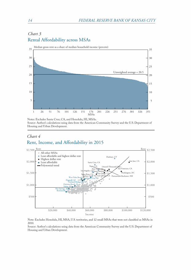
Chart 3 shows rental affordability in 2015 by MSA. Specifically, the chart shows the ratio of annualized gross median rent to median household income across MSAs. The data reveal significant variation in rental housing affordability across MSAs, where affordability is mea-sured as expenditure on rent relative to income.

In 2015, the median expenditure on rental housing as a share of household median income (hereafter, “expenditure share”) ranged from 13.5 percent in Jefferson City, MO, to 34.6 percent in Santa Cruz, CA. That is, median rent consumed 13.5 percent of gross median household income in Jefferson City and 34.6 percent of gross median household income in Santa Cruz. However, Santa Cruz is an outlier. The second-least affordable MSAs, Los Angeles, CA, and West Palm Beach, FL, had expenditure shares of 29.7 percent in 2015.

MSAs with high rents are not necessarily unaffordable. Chart 4 shows that rents and income tend to move together, fitting tightly around a (polynomial) regression line. Many MSAs with very high me-dian rents—such as San Jose ($1,965), San Francisco, CA ($1,708), and Washington, DC ($1,574)—also had high median incomes and thus were not among the least affordable. San Jose provides a salient example. In 2015, median rent in San Jose was the highest in the na-tion, but median household income was also the highest in the nation at $101,980, giving San Jose an expenditure share of 23.1 percent. In

14 FEDERAL RESERVE BANK OF KANSAS CITY

Chart 3Rental Affordability across MSAs

Chart 4Rent, Income, and Affordability in 2015

Notes: Excludes Santa Cruz, CA, and Honolulu, HI, MSAs.Source: Author’s calculations using data from the American Community Survey and the U.S. Department of Housing and Urban Development.

Note: Excludes Honolulu, HI, MSA, U.S. territories, and 12 small MSAs that were not classified as MSAs in 2010.Source: Author’s calculations using data from the American Community Survey and the U.S. Department of Housing and Urban Development.

5

10

15

20

25

30

35

5

10

15

20

25

30

35

1 26 51 76 101 126 151 176 201 226 251 276 301 326 351 MSAs

Unweighted average = 20.5

Median gross rent as a share of median household income (percent)

$500

$1,000

$1,500

$2,000

$2,500

$500

$1,000

$1,500

$2,000

$2,500

$20,000 $40,000 $60,000 $80,000 $100,000 $120,000

All other MSAs

Rent Rent

Least affordable and highest dollar rent Highest dollar rent Least affordable Polynomial trend

Danbury, CT

Santa Cruz, CA

New York, NY Santa Barbara, CA Los Angeles, CA

San Diego, CA San Luis Obispo, CA

San Jose, CA

San Francisco, CA

Washington, DC

Oxnard-Thousand Oaks-

Portsmouth-Rochester, NH

Napa, CA

Santa Rosa, CA Salinas, CA

Atlantic City, NJ West Palm Beach, FL Flagstaff, AZ

Vineland-Bridgeton, NJ Daytona Beach, FL Yuma, AZ

Hot Springs, AR Brownsville, TX

Income

ECONOMIC REVIEW • FOURTH QUARTER 2016 15

2015, 64 MSAs were less affordable than San Jose by this accounting. Similarly, 63 MSAs were less affordable than San Francisco, and 162 MSAs were less affordable than Washington, DC.

Likewise, MSAs with low rents are not necessarily affordable. In Hot Springs, AR, for example, median rent in 2015 was only $850—but in-come was $37,013, giving Hot Springs an expenditure share of 27.6 per-cent, thereby making it one of the least affordable MSAs in the nation. Similarly, in Brownsville, TX, median rent was among the lowest in the nation at $710, but its low median income of $34,074 gave Brownsville a relatively high expenditure share of 24.8 percent. Brownsville was among the least affordable MSAs with populations greater than 250,000 and ranked as 34th-least affordable across all 355 MSAs.

One caveat to these characterizations is that there is a wide distri-bution of income in all cities. For example, for any given level of in-come, rent would be less affordable in San Jose than in Hot Springs. The rankings here offer insight only into the relative affordability of different MSAs for households earning the median income in that MSA.

Changes in affordability over time

Housing affordability for median-income households varies over time as well as over MSA. To assess whether housing has grown more or less affordable for these households recently, I measure affordability over time as a percentage change in the expenditure share. Arithmeti-cally, the percentage change in expenditure share, (E), is equal to the growth in rent, (R), minus the growth in income, (I):

%ΔE =E2015 −E2010

E2010

=( R2015 / I 2015 ) −( R2010 / I 2010 )

R2010 / I 2010

=R2015 / R2010

I 2015 / I 2010

−1 =%ΔR −%ΔI .

Although much of the public discourse around rental affordability has focused on the rise in rents, the above equation shows that rent growth and income growth have equal (and opposite) effects on chang-es in affordability.

Nationally, rents became somewhat less affordable from 2010 to 2014, as the expenditure share rose from 20.5 percent to 20.9 percent. Rent became more affordable in 2015, however, as the national expen-diture share dropped to 20.6. The decline in the expenditure share in 2015 was due entirely to higher income.

16 FEDERAL RESERVE BANK OF KANSAS CITY

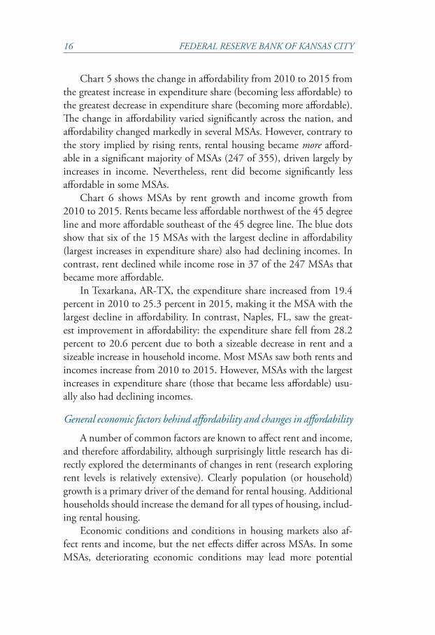
Chart 5 shows the change in affordability from 2010 to 2015 from the greatest increase in expenditure share (becoming less affordable) to the greatest decrease in expenditure share (becoming more affordable). The change in affordability varied significantly across the nation, and affordability changed markedly in several MSAs. However, contrary to the story implied by rising rents, rental housing became more afford-able in a significant majority of MSAs (247 of 355), driven largely by increases in income. Nevertheless, rent did become significantly less affordable in some MSAs.

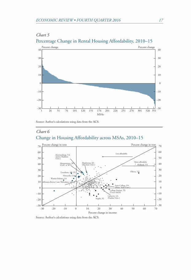
Chart 6 shows MSAs by rent growth and income growth from 2010 to 2015. Rents became less affordable northwest of the 45 degree line and more affordable southeast of the 45 degree line. The blue dots show that six of the 15 MSAs with the largest decline in affordability (largest increases in expenditure share) also had declining incomes. In contrast, rent declined while income rose in 37 of the 247 MSAs that became more affordable.

In Texarkana, AR-TX, the expenditure share increased from 19.4 percent in 2010 to 25.3 percent in 2015, making it the MSA with the largest decline in affordability. In contrast, Naples, FL, saw the great-est improvement in affordability: the expenditure share fell from 28.2 percent to 20.6 percent due to both a sizeable decrease in rent and a sizeable increase in household income. Most MSAs saw both rents and incomes increase from 2010 to 2015. However, MSAs with the largest increases in expenditure share (those that became less affordable) usu-ally also had declining incomes.

General economic factors behind affordability and changes in affordability

A number of common factors are known to affect rent and income, and therefore affordability, although surprisingly little research has di-rectly explored the determinants of changes in rent (research exploring rent levels is relatively extensive). Clearly population (or household) growth is a primary driver of the demand for rental housing. Additional households should increase the demand for all types of housing, includ-ing rental housing.

Economic conditions and conditions in housing markets also af-fect rents and income, but the net effects differ across MSAs. In some MSAs, deteriorating economic conditions may lead more potential

ECONOMIC REVIEW • FOURTH QUARTER 2016 17

Chart 5Percentage Change in Rental Housing Affordability, 2010–15

Chart 6Change in Housing Affordability across MSAs, 2010–15

Source: Author’s calculations using data from the ACS.

Source: Author’s calculations using data from the ACS.

–30

–20

–10

0

10

20

30

40

1 –30

–20

–10

0

10

20

30

40

26 51 76 101 126 151 176 201 226 251 276 301 326 351 MSAs

Percent change Percent change

–30

–20

–10

0

10

20

30

40

50

60

70

-30 -20 -10 0 10 20 30 40 50 60 70

Percent change in rent

–30

–20

–10

0

10

20

30

40

50

60

70 Percent change in rent

Percent change in income

Less a�ordable

More a�ordable Manhattan, KS (KS State Univ.)

Morgantown, WV (Univ. of WV)

Harrisonburg, VA (James Madison Univ.)

Texarkana, AR-TX

Hinesville, GA

Midland, TX

Houma-Bayou Cane-�ibodaux, LA

Warner Robins, GA

Odessa, TX

College Station, TX (Texas A&M)

Naples, FL Lafayette, LA (Purdue Univ.)

State College, PA (Penn. State Univ.)

18 FEDERAL RESERVE BANK OF KANSAS CITY

homeowners to rent, due either to reduced income, a negative outlook, or a desire for the increased geographic mobility that comes with rent-ing. This process should put upward pressure on demand, and hence rent, all else equal. But in other MSAs, poor economic conditions may persuade residents to seek out better opportunities in other locations.

While personal income directly affects housing affordability, as measured by the expenditure share, changes in personal income may change rents as well, with the net effect varying across MSAs. An in-crease in personal income may induce some residents, including rent-ers, to commit more dollars to housing, pushing up rents. Increased household formation arising from increased income may also increase the demand for rental units and therefore rent. Alternatively, increased personal income may lead some residents away from rental housing as they purchase homes.

A decline in home prices, as occurred in most areas during the re-cent housing bust, would likely lead to higher rates of delinquency and foreclosure, driving some affected households out of owner-occupancy and into rental housing. Disruption in owner-occupied housing mar-kets and economic challenges often occur simultaneously, as in the re-cent recession and financial crisis.

The role of smaller one-industry MSAs

While changes in rental affordability across MSAs arise from a num-ber of common economic factors, a more detailed analysis of the data suggests that some of the more extreme changes occur in smaller MSAs. This may not be surprising since local factors are likely much more pro-nounced in MSAs with small populations. For example, five of the 15 least-affordable MSAs in 2015 had populations below 250,000, and 10 had populations below 500,000. In addition, 12 of the 15 MSAs with the most significant declines in affordability from 2010 to 2015 had populations below 250,000.13

In particular, it is much more likely that smaller MSAs—as op-posed to larger MSAs—are dominated by a single industry. As a re-sult, affordability will depend to a large extent on what happens to the particular industry. I find that many of the MSAs with extreme changes in affordability are dependent on military bases, subject to commodity booms, or home to universities.

ECONOMIC REVIEW • FOURTH QUARTER 2016 19

Military bases. Military bases are located in three of the 15 MSAs that saw the greatest increase in expenditure share (declining afford-ability) from 2010 to 2015: Hinesville, GA (the Army’s Fort Stewart); Texarkana, AR-TX (Red River Army Depot); and Warner Robins, GA (Robins Air Force Base) (Chart 6). Other MSAs with a large military presence also saw significant increases in expenditure share. Specifi-cally, Fayetteville, NC (the Army’s Fort Bragg), saw the 18th-largest increase in expenditure share across all MSAs, while Yuma, AZ (Ma-rine Corps Air Station), saw the 32nd-largest increase in expenditure share.14 Manhattan, KS, among the MSAs with the largest increase in expenditure share from 2010 to 2015, is important to the analysis of rent affordability in part because it hosts a large university, but also because it abuts a very large military base (the Army’s Fort Riley in Junction City, KS).

Of course, whether a military MSA saw an increase or decrease in affordability depends on base closures, realignments, and troop deployments.15 For example, Goldsboro, NC (Seymour-Johnson Air Force Base), and Sumter, SC (Shaw Air Force Base), saw substantial increases in expenditure share in the 2010–14 period but saw expen-diture shares fall sharply from 2014 to 2015, making rent much more affordable over the course of the past year.

Commodity MSAs. Smaller MSAs dependent on energy saw large rent increases in recent years, though the overall effect of these in-creases on affordability depended on income. From 2010 to 2014, several MSAs received substantial economic benefits associated with the booming energy sector.16 Odessa, TX, which is highly dependent on crude oil production, experienced an influx of workers and a sub-sequent 64 percent increase in median rent from $638 per month in 2010 to $1,049 per month in 2014. This increase in rent was the larg-est among all MSAs. And while the energy workers were well-paid—median household income in Odessa increased 39 percent over this pe-riod—the increase in rent far exceeded the increase in income, causing affordability to decline. Specifically, the expenditure share increased from 18.1 percent in 2010 to 21.4 percent in 2014.

Midland, TX, which is roughly 20 miles from Odessa, saw the second-greatest increase in rent at 43 percent, rising from $848 in 2010 to $1,210 in 2014. But in contrast to Odessa, Midland became

20 FEDERAL RESERVE BANK OF KANSAS CITY

more affordable over this period due to a substantial increase in median income of 46 percent.

Another energy MSA, Houma-Bayou Cane-Thibodaux, LA, was among the 15 MSAs with the greatest increase in expenditure share from 2010 to 2014. Rent increased by 22.5 percent in Houma-Bayou Cane-Thibodaux over 2010–14. However, unlike most energy boom cities, income declined by 6.4 percent over the same period, exacer-bating the effects of steeply increasing rent. The declining income in Houma-Bayou Cane-Thibodaux is likely a result of the Deepwater Ho-rizon disaster in 2010, which initially decimated the area economically (Greater New Orleans Regional Economic Alliance; Batte 2015a; Gor-don; Batte 2015b). While longer-term “doomsday” predictions for the area economy never materialized, the oil industry did not fully recover until 2014, due in large part to a temporary moratorium on offshore drilling there. Moreover, commercial fishing is a substantial share of the Houma-Bayou Cane-Thibodaux economy, and that industry has not yet recovered.

Much has changed in energy MSAs since 2014. Oil prices (WTI, monthly) have fallen sharply, from $105.70 in June 2014 to $30.32 in February 2016 (U.S. Energy Information Administration). The decline in oil prices has been accompanied by a significant decline in energy ac-tivity (Federal Reserve Bank of Kansas City). In 2014, three of the top 10 fastest-growing “small MSAs” were energy-driven, including Mid-land (second), Odessa (third), and Houma-Bayou Cane-Thibodaux (eighth). But from 2014 to 2015, median rent fell in Odessa from $1,083 to $989 (−8.7 percent). In contrast, median income grew by 11.5 percent that year. In Houma-Bayou Cane-Thibodaux, LA, median rent fell from $823 to $794 (−3.5 percent), but again, median income grew moderately faster. Midland, TX, saw both rents and income con-tinue to increase from 2014 to 2015, but at a much slower rate.

Universities. In addition to MSAs that are home to military bases or are subject to energy price booms and busts, universities may also explain changes in affordability in some MSAs. The data in Chart 6 reveal that three of the 15 MSAs with greatest increase in rent expenditure share from 2010 to 2014 are hosts to large universities: Kansas State University in Manhattan, KS; University of West Virginia in Morgantown, WV; and James Madison University in Harrisonburg, VA. This pattern holds for

ECONOMIC REVIEW • FOURTH QUARTER 2016 21

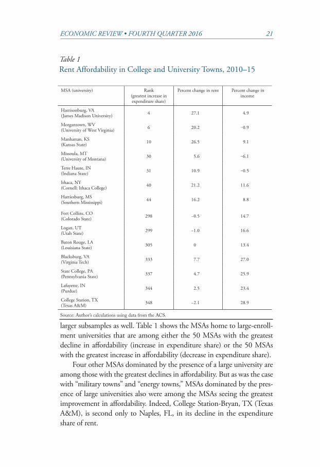
Table 1Rent Affordability in College and University Towns, 2010–15

MSA (university) Rank (greatest increase in expenditure share)

Percent change in rent Percent change in income

Harrisonburg, VA(James Madison University) 4 27.1 4.9

Morgantown, WV(University of West Virginia) 6 20.2 ‒0.9

Manhattan, KS(Kansas State) 10 26.5 9.1

Missoula, MT(University of Montana) 30 5.6 ‒6.1

Terre Haute, IN(Indiana State) 31 10.9 ‒0.5

Ithaca, NY(Cornell; Ithaca College) 40 21.2 11.6

Hattiesburg, MS (Southern Mississippi) 44 16.2 8.8

Fort Collins, CO(Colorado State) 298 −0.5 14.7

Logan, UT(Utah State) 299 −1.0 16.6

Baton Rouge, LA(Louisiana State) 305 0 13.4

Blacksburg, VA(Virginia Tech) 333 7.7 27.0

State College, PA(Pennsylvania State) 337 4.7 25.9

Lafayette, IN(Purdue) 344 2.5 23.4

College Station, TX(Texas A&M) 348 −2.1 28.9

larger subsamples as well. Table 1 shows the MSAs home to large-enroll-ment universities that are among either the 50 MSAs with the greatest decline in affordability (increase in expenditure share) or the 50 MSAs with the greatest increase in affordability (decrease in expenditure share).

Four other MSAs dominated by the presence of a large university are among those with the greatest declines in affordability. But as was the case with “military towns” and “energy towns,” MSAs dominated by the pres-ence of large universities also were among the MSAs seeing the greatest improvement in affordability. Indeed, College Station-Bryan, TX (Texas A&M), is second only to Naples, FL, in its decline in the expenditure share of rent.

Source: Author’s calculations using data from the ACS.

22 FEDERAL RESERVE BANK OF KANSAS CITY

Several factors likely play into the effect of a large university pres-ence on MSAs. Because rents in some university towns are getting much more affordable and rents in some are getting much less affordable, national trends are unlikely to be insightful. Instead, further research is needed to investigate location-specific trends, such as enrollments, higher education investments, and state and local policies, to better understand how universities affect rental affordability across MSAs.

IV. Conclusion

In recent years, renters and their advocates (who typically represent LMI households) have expressed concerns about significant increases in residential rents and associated declines in affordability. Nationally, data show that residential rents have become modestly less affordable for the median household in recent years. Similarly, an analysis of hous-ing wages indicates that many LMI households are facing less afford-able rents, but that MSAs that initially were the least affordable gener-ally are the MSAs that have seen the greatest increases in affordability (decreasing expenditure shares).

Middle-income households, as measured by median rent and in-come, are facing rapidly declining affordability in some MSAs, but have enjoyed much more affordable housing over the last five years in a large majority of MSAs. Analysis at the MSA level reveals that afford-ability and changes in affordability have varied widely and that only a small subset of MSAs have seen significant changes in affordability.

Several factors have likely driven trends in affordability across MSAs. In addition to the “usual suspects,” such as population and income growth and economic and housing conditions, MSAs at the extremes of affordability, especially those with extreme changes in af-fordability, are likely to be smaller and dominated by energy activity or institutions such as military bases and large universities.

ECONOMIC REVIEW • FOURTH QUARTER 2016 23

Endnotes

1The most recent count puts the rate of homelessness in the United States at 17.7 per 10,000 residents (HUD). Among the homeless, about 27 percent of individuals are unsheltered, with the remainder taking refuge in emergency shelters or transitional housing.

2Public housing had its genesis in the New Deal. It was intended to be fund-ed by rents, much like private rental units (although the construction of public housing units was subsidized). As public housing began to deteriorate over time, significantly higher spending on maintenance was required. Housing authorities responded by raising rents. In response to tenant backlash, Congress passed the Brooke Amendment, which altered the financing model for public housing. Spe-cifically, it set a threshold for public housing costs (including utilities) as a share of income, with the federal government filling the gap. Husock provides a useful, succinct history of the Brooke Amendment.

3Assisted housing programs like the Section 8 Voucher Program subsidize market-rate rental units, and Fair Market Rent is a market rate (it excludes non-market rental housing in its computation). In some MSAs (17 in 2016), Fair Market Rent is set at the 50th percentile to ensure that a sufficient supply of rental housing is available to program participants (to qualify for subsidies, rent cannot exceed the Fair Market Rent). A limited availability of qualified homes at the 40th percentile usually arises in areas where voucher recipients are geograph-ically more concentrated. HUD still publishes 40th percentile rents for these MSAs, but they are not used for the Housing Choice Voucher program. See, for example, for Baltimore: https://www.huduser.gov/portal/datasets/fmr/fmrs/FY2016_code/2016summary.odn?&year=2016&fmrtype=Final&cbsasub=METRO12580M12580.

4Rank order in this case is the distribution of income or housing cost from the lowest to the highest (or vice versa). If housing units are selected in the same rank order as income, then the household with the lowest income would rent the lowest-cost dwelling, the household with the second-lowest income would rent the second lowest cost dwelling; and so on.

5Most states (28) and the District of Columbia have legislated minimum wages above the federal minimum wage—the highest being the District of Co-lumbia, where the minimum wage is currently $11.50. Some localities also have minimum wages. Employers are required to pay the highest of federal, state, and local minimums.

6These include San Francisco (see http://sfgov.org/olse/minimum-wage-ordinance-mwo), Los Angeles (http://wagesla.lacity.org/sites/g/files/wph471/f/Los%20Angeles%20Minimum%20Wage%20Ordinance%20184320.pdf ), and Seattle (http://www.seattle.gov/Documents/Departments/LaborStandards/OLS-FactSheets-MWO.pdf ).

24 FEDERAL RESERVE BANK OF KANSAS CITY

7The median wage used here is from the BLS National Compensation Sur-vey, Employer Costs for Employee Compensation, Wages & Salaries component.

8There are no statutory limits on the number of hours a person may work in a week.

9Specifically, the margin of error is less than 50 percent of the estimate itself. There are a small number of exceptions.

10A household with median income does not necessarily pay median rent. However, it is treated as if it does for the purpose of this analysis.

11CPI Rent on Primary Residence is the most commonly used measure of typical rent at the national level, but its regional coverage is limited to 25 large MSAs, an inadequate number for a study of affordability over MSAs.

12A large increase in luxury apartments has been common among larger cities recently. Yardi Matrix apartment information service suggests that 75 percent of all new apartments constructed in 2015 were “high-end” (Balient; see also Lahart).

13The three exceptions are Visalia-Porterville, CA; Olympia, WA; and Se-attle, WA.

14Most military bases host multiple military units.15The Base Realignment and Closure Commission recommendations signifi-

cantly reduced personnel at some bases, possibly due to closure, but significantly increased personnel in others.

16Crude oil prices climbed from about $45 per barrel in December 2008 to a (monthly average) peak of about $107 in February 2014.

ECONOMIC REVIEW • FOURTH QUARTER 2016 25

References

American Psychological Association. 2010. “Health and Homelessness.” Fact Sheet. Available at https://www.apa.org/pi/ses/resources/publications/home-lessness-health.pdf.

Balient, Nadia. 2016. “75% of All New Apartments in 2015 Were High-End, 14 U.S. Cities Saw No New Affordable Rentals.” Rent Café Blog. Available at http://www.rentcafe.com.

Bassuk, Ellen L., Lenore Rubin, and Alison S. Lauriat. 1986. “Characteristics of Sheltered Homeless Families,” American Journal of Public Health, vol. 76, no. 9, pp. 1097–1101. Available at https://doi.org/10.2105/ajph.76.9.1097.

Batte, Jacob. 2015a. “Five Years Later, Oil Spill’s Environmental Impact Debated,” Houma Courier, April 18. Available at http://www.houmatoday.com/article/DA/20150418/News/608081374/HC/.

———. 2015b. “5 Years Later: Could the BP Oil Spill Happen Again?” Houma Courier, April 20. Available at http://www.houmatoday.com/news/20150420/5-years-later-could-the-bp-oil-spill-happen-again.

Clarkberg, Marin. 1999. “The Household Workweek.” The Time-Squeeze in American Families: From Causes to Solutions. Futurework: Trends and Chal-lenges in the 21st Century, U.S. Department of Labor. Paper presented at the Economic Policy Institute symposium, June. Available at https://www.dol.gov/dol/aboutdol/history/herman/reports/futurework/conference/families/workweek.htm.

Craig, Courtney. 2014. “What’s the Most Expensive Town in the U.S.? The An-swer May Surprise You.” Apartment Guide Blog, February 17. Available at http://www.apartmentguide.com/blog/williston-nd/.

Desmond, Matthew, and Rachel Tolbert Kimbro. 2015. “Eviction’s Fallout: Housing, Hardship, and Health.” Social Forces, vol. 94, no. 1, pp. 295–324. Available at https://doi.org/10.1093/sf/sov044.

Dickstein, Corey. 2015. “Fort Stewart’s 2nd Brigade Inactivates as Army Draw-down Continues,” Savannah Morning News, January 15. Available at http://savannahnow.com/news/2015-01-15/fort-stewarts-2nd-brigade-inactivates-army-drawdown-continues.

Divringi, Eileen. 2015. “Affordability and Availability of Rental Housing in the Third Federal Reserve District: 2015.” Federal Reserve Bank of Philadelphia, Cascade Focus, February.

Dunne, Timothy. 2012. “Household Formation and the Great Recession.” Federal Reserve Bank of Cleveland, Economic Commentary, No. 2012-12, August 23.

Fallah, Belal, Mark D. Partridge, and Dan S. Rickman. 2014. “Geography and High-Tech Employment Growth in US Counties.” Journal of Economic Ge-ography, vol. 14, no. 4, pp. 683–720. Available at https://doi.org/10.1093/jeg/lbt030.

Fama, Eugene F., and Kenneth R. French. 1992. “The Cross-Section of Expected Returns,” Journal of Finance, vol. 47, pp. 427–466.

Fannie Mae. 2016. “Multifamily Market Commentary–July 2016.” Available at http://fanniemae.com/resources/file/research/emma/pdf/MF_Market_Com-mentary_071916.pdf.

26 FEDERAL RESERVE BANK OF KANSAS CITY

Feickert, Andrew. 2014. “Army Drawdown and Restructuring: Background and Issues for Congress.” Congressional Research Service, February 28.

Gordon, Aaren. 2015. “After Oil Spill, Local Economy Defies Doomsday Fore-casts,” Houma Courier, April 19. Available at http://www.houmatoday.com/news/20150419/after-oil-spill-local-economy-defies-doomsday-forecasts.

Greater New Orleans Inc. Regional Economic Alliance. 2010. “A Study of the Impact of the Deepwater Horizon Oil Spill,” October 15.

Honig, Marjorie, and Randall K. Filer. 1993. “Causes of Intercity Variation in Homelessness.” American Economic Review, vol. 83, no. 1, pp. 248–255.

Husock, Howard. 2015. “How Brooke Helped Destroy Public Housing.” Forbes, January 8.

Immergluck, Dan, Ann Carpenter, and Abram Lueders. 2016. “Declines in Low-Cost Rented Housing Units in Eight Large Southeastern Cities.” Federal Re-serve Bank of Atlanta Community & Economic Development Discussion Paper No. 03-16, May.

Johnstone, Melissa, Cameron Parsell, Jolanda Jetten, Genevieve Dingel, and Zoe Walter. 2015. “Breaking the Cycle of Homelessness: Housing Stability and Social Support as Predictors of Long-Term Well-Being.” Housing Studies, vol. 31, no. 4, pp. 1–17. Available at https://doi.org/10.1080/02673037.2015.1092504.

Joint Center for Housing Studies, Harvard University. 2013. “America’s Rental Housing: Evolving Markets and Needs.”

Kotkin, Joel. 2014. “America’s Fastest-Growing Small Cities,” Forbes, September 3.Kotkin, Joel, and Mark Schill. 2015. “The Valley and the Upstarts: The Cities

Creating the Most Tech Jobs,” Forbes, April 14.Lahart, Justin. 2016. “Apartment Boom Needs Cooling-Off Period,” The Wall

Street Journal, June 16.Long, David, John Rio, and Jeremy Rosen. 2007. “Employment and Income Sup-

ports for Homeless People.” Toward Understanding Homelessness: The 2007 National Symposium on Homelessness Research, March 1–2.

Mandel, Michael. 2013. “The PPI Tech/Info Job Ranking.” Progressive Policy In-stitute, October.

Moore, Tech. Sgt. Tammie. 2010. “New Reserve Group Stands Up at Seymour Johnson,” Public Affairs, 4th Fighter Wing, Official Web Site of the U.S. Air-force, March 30. Archived at https://web.archive.org/web/20111219150753/http://www.af.mil/news/story.asp?id=123197295.

Muro, Mark, Jonathan Rothwell, Scott Andes, Kenan Fikri, and Siddharth Kulkar-ni. 2015. “America’s Advanced Industries: What They Are, Where They Are, and Why They Matter.” Brookings Institution, Metropolitan Policy Pro-grams, February.

National Association of Realtors. Housing Affordability Index [datafile].National Low-Income Housing Coalition. 2016. “Out of Reach 2016.” Washing-

ton, DC.Numen, Sandra J., and C. Scott Holupka. 2014. “Affordable Housing Is Associ-

ated with Greater Spending on Child Enrichment and Stronger Cognitive Development.” How Housing Matters, MacArthur Foundation, June.

Pew Charitable Trusts. 2016. “Household Expenditures and Income: Balanc-ing Family Finances in Today’s economy.” March. Available at http://www.

ECONOMIC REVIEW • FOURTH QUARTER 2016 27

pewtrusts.org/~/media/assets/2016/03/household_expenditures_and_in-come.pdf.

Rafferty, Yvonne, and Marybeth Shinn. 1991. “The Impact of Homelessness on Children,” American Psychologist, vol. 46, no. 11, pp. 1170–1179. Available at https://doi.org/10.1037//0003-066x.46.11.1170.

Rappaport, Jordan. 2008. “The Affordability of Homeownership to Middle-In-come Americans.” Federal Reserve Bank of Kansas City, Economic Review, vol. 93, no. 4, pp. 65–95.

Skobba, Kimberly, and Edward G. Goetz. 2015. “Doubling Up and the Erosion of Social Capital among Very Low Income Households.” International Journal of Housing Policy, vol. 15, no. 12, pp. 127–147. Available at https://doi.org/10.1080/14616718.2014.961753.

U.S. Army. “Basic Pay: Active Duty Soldiers,” Available at http://www.goarmy.com/benefits/money/basic-pay-active-duty-soldiers.html.

U.S. Bureau of Labor Statistics. 2016. Consumer Expenditure Survey. Table 1702. Available at http://www.bls.gov/cex/2015/combined/tenure.pdf.

———. Current Population Survey, Usual Weekly Earnings. Extracted from Ha-ver Analytics DLXG3.

U.S. Department of Defense. 2012. Fiscal Year 2013 Budget Request, February. Available at http://comptroller.defense.gov/Portals/45/Documents/defbud-get/fy2013/FY2013_Budget_Request_Overview_Book.pdf.

U.S. Department of Housing and Urban Development. 2015. “The 2015 Annual Homeless Assessment Report (AHAR) to Congress, Part 1: Point-in-Time Estimates of Homelessness,” Washington, DC, November.

———. 2007. “Fair Market Rents for the Section 8 Housing Assistance Pay-ments Program.” Office of Policy Development & Research, July. Available at https://www.huduser.gov/portal/datasets/fmr/fmrover_071707R2.doc.

Zellner, Arnold. 1962. “An Efficient Method of Estimating Seemingly Unrelated Regressions and Tests for Aggregation Bias,” Journal of the American Sta-tistical Association, vol. 57, no. 298, pp. 348–368. Available at https://doi.org/10.2307/2281644.