Residual Ratio Tracking for Estimating Attenuation in

From the SIGGRAPH Asia 2014 conference proceedings.

Residual Ratio Tracking for Estimating Attenuation in Participating Media

Jan Novak1,2 Andrew Selle1 Wojciech Jarosz2

1Walt Disney Animation Studios 2Disney Research Zurich

(a) Path traced light transport in clouds

RMSE: 0.043RMSE: 0.043RMSE: 0.043RMSE: 0.043RMSE: 0.043RMSE: 0.043RMSE: 0.043RMSE: 0.043RMSE: 0.043RMSE: 0.043RMSE: 0.043RMSE: 0.043RMSE: 0.043RMSE: 0.043RMSE: 0.043RMSE: 0.043RMSE: 0.043RMSE: 0.043RMSE: 0.043RMSE: 0.043RMSE: 0.043RMSE: 0.043RMSE: 0.043RMSE: 0.043RMSE: 0.043RMSE: 0.043RMSE: 0.043RMSE: 0.043RMSE: 0.043RMSE: 0.043RMSE: 0.043RMSE: 0.043RMSE: 0.043RMSE: 0.043RMSE: 0.043RMSE: 0.043RMSE: 0.043RMSE: 0.043RMSE: 0.043RMSE: 0.043RMSE: 0.043RMSE: 0.043RMSE: 0.043RMSE: 0.043RMSE: 0.043RMSE: 0.043RMSE: 0.043RMSE: 0.043RMSE: 0.043RMSE: 0.043RMSE: 0.043Cost: 51.5 MCost: 51.5 MCost: 51.5 MCost: 51.5 MCost: 51.5 MCost: 51.5 MCost: 51.5 MCost: 51.5 MCost: 51.5 MCost: 51.5 MCost: 51.5 MCost: 51.5 MCost: 51.5 MCost: 51.5 MCost: 51.5 MCost: 51.5 MCost: 51.5 MCost: 51.5 MCost: 51.5 MCost: 51.5 MCost: 51.5 MCost: 51.5 MCost: 51.5 MCost: 51.5 MCost: 51.5 MCost: 51.5 MCost: 51.5 MCost: 51.5 MCost: 51.5 MCost: 51.5 MCost: 51.5 MCost: 51.5 MCost: 51.5 MCost: 51.5 MCost: 51.5 MCost: 51.5 MCost: 51.5 MCost: 51.5 MCost: 51.5 MCost: 51.5 MCost: 51.5 MCost: 51.5 MCost: 51.5 MCost: 51.5 MCost: 51.5 MCost: 51.5 MCost: 51.5 MCost: 51.5 MCost: 51.5 MCost: 51.5 MCost: 51.5 M

RMSE: 0.123RMSE: 0.123RMSE: 0.123RMSE: 0.123RMSE: 0.123RMSE: 0.123RMSE: 0.123RMSE: 0.123RMSE: 0.123RMSE: 0.123RMSE: 0.123RMSE: 0.123RMSE: 0.123RMSE: 0.123RMSE: 0.123RMSE: 0.123RMSE: 0.123RMSE: 0.123RMSE: 0.123RMSE: 0.123RMSE: 0.123RMSE: 0.123RMSE: 0.123RMSE: 0.123RMSE: 0.123RMSE: 0.123RMSE: 0.123RMSE: 0.123RMSE: 0.123RMSE: 0.123RMSE: 0.123RMSE: 0.123RMSE: 0.123RMSE: 0.123RMSE: 0.123RMSE: 0.123RMSE: 0.123RMSE: 0.123RMSE: 0.123RMSE: 0.123RMSE: 0.123RMSE: 0.123RMSE: 0.123RMSE: 0.123RMSE: 0.123RMSE: 0.123RMSE: 0.123RMSE: 0.123RMSE: 0.123RMSE: 0.123RMSE: 0.123Cost: 1.22 GCost: 1.22 GCost: 1.22 GCost: 1.22 GCost: 1.22 GCost: 1.22 GCost: 1.22 GCost: 1.22 GCost: 1.22 GCost: 1.22 GCost: 1.22 GCost: 1.22 GCost: 1.22 GCost: 1.22 GCost: 1.22 GCost: 1.22 GCost: 1.22 GCost: 1.22 GCost: 1.22 GCost: 1.22 GCost: 1.22 GCost: 1.22 GCost: 1.22 GCost: 1.22 GCost: 1.22 GCost: 1.22 GCost: 1.22 GCost: 1.22 GCost: 1.22 GCost: 1.22 GCost: 1.22 GCost: 1.22 GCost: 1.22 GCost: 1.22 GCost: 1.22 GCost: 1.22 GCost: 1.22 GCost: 1.22 GCost: 1.22 GCost: 1.22 GCost: 1.22 GCost: 1.22 GCost: 1.22 GCost: 1.22 GCost: 1.22 GCost: 1.22 GCost: 1.22 GCost: 1.22 GCost: 1.22 GCost: 1.22 GCost: 1.22 G

(b) Delta tracking



(c) Ratio tracking



(d) Residual ratio tracking

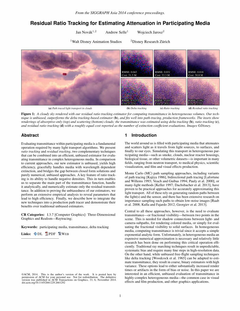
Figure 1: A cloudy sky rendered with our residual ratio tracking estimator for computing transmittance in heterogeneous volumes. Our tech-nique is unbiased, outperforms the delta tracking-based estimator (b), and fits well into path-tracing, production frameworks. The insets showrenderings of absorptive-only (top) and scattering (bottom) clouds; the transmittance was estimated using delta tracking (b), ratio tracking (c),and residual ratio tracking (d) with a roughly equal cost reported as the number of extinction coefficient evaluations. Images ©Disney.

Abstract

Evaluating transmittance within participating media is a fundamentaloperation required by many light transport algorithms. We presentratio tracking and residual tracking, two complementary techniquesthat can be combined into an efficient, unbiased estimator for evalu-ating transmittance in complex heterogeneous media. In comparisonto current approaches, our new estimator is unbiased, yields highefficiency, gracefully handles media with wavelength dependentextinction, and bridges the gap between closed form solutions andpurely numerical, unbiased approaches. A key feature of ratio track-ing is its ability to handle negative densities. This in turn enablesus to separate the main part of the transmittance function, handleit analytically, and numerically estimate only the residual transmit-tance. In addition to proving the unbiasedness of our estimators, weperform an extensive empirical analysis to reveal parameters thatlead to high efficiency. Finally, we describe how to integrate thenew techniques into a production path tracer and demonstrate theirbenefits over traditional unbiased estimators.

CR Categories: I.3.7 [Computer Graphics]: Three-DimensionalGraphics and Realism—Raytracing;

Keywords: participating media, transmittance, delta tracking

Links: DL PDF WEB

©ACM, 2014. This is the author’s version of the work. It is posted here bypermission of ACM for your personal use. Not for redistribution. The definitiveversion was published in ACM Transactions on Graphics, 33, 6, November 2014.doi.acm.org/10.1145/2661229.2661292

1 Introduction

The world around us is filled with participating media that attenuatesand scatters light as it travels from light sources, to surfaces, andfinally to our eyes. Simulating this transport in heterogeneous par-ticipating media—such as smoke, clouds, nuclear reactor housings,biological tissue, or other volumetric datasets—is important in manyfields, ranging from neutron transport, to medical physics, scientificvisualization, and film and visual effects production.

Monte Carlo (MC) path sampling approaches, including variantsof path tracing [Kajiya 1986], bidirectional path tracing [Lafortuneand Willems 1993; Veach and Guibas 1994; Pauly et al. 2000], ormany-light methods [Keller 1997; Dachsbacher et al. 2013], haveproven to be practical approaches for accurately approximating thislight transport. All of these rely on generating random paths betweenthe light(s) and the sensor, and there has been extensive research onimportance sampling such paths to obtain low-noise images [Raabet al. 2008; Kulla and Fajardo 2012; Georgiev et al. 2013].

Central to all these approaches, however, is the need to evaluatetransmittance—or fractional visibility—between two points in thescene. This is needed for shadow connections between light- andcamera-subpaths, for rendering colored media, or simply for eval-uating the fractional visibility to solid surfaces. In homogeneousmedia, computing transmittance is trivial since it accepts a simpleexponential analytic form. Unfortunately, in heterogeneous media anexpensive numerical approximation is necessary and relatively littleresearch has been done on performing this critical operation effi-ciently. Traditional ray marching techniques result in unpredictable,systematic bias and require many fine steps in high-resolution data.On the other hand, while unbiased free-flight sampling techniqueslike delta tracking [Woodcock et al. 1965] can be adapted to esti-mate transmittance, they result in coarse, binary estimators with highvariance. These options lead to either substantially increased rendertimes or artifacts in the form of bias or noise. In this paper we areinterested in an efficient, unbiased evaluation of transmittance inhighly-complex heterogeneous media—the common case in visualeffects and film production, and other graphics applications.

1

http://doi.acm.org/10.1145/2661229.2661292

http://portal.acm.org/ft_gateway.cfm?id=2661292&type=pdf

http://cs.dartmouth.edu/~wjarosz/publications/novak14residual.html

http://doi.acm.org/10.1145/2661229.2661292

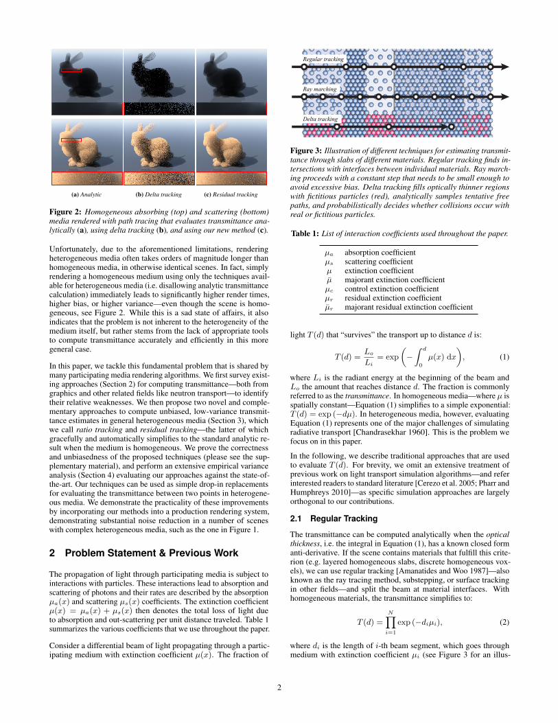
(a) Analytic (b) Delta tracking (c) Residual tracking

Figure 2: Homogeneous absorbing (top) and scattering (bottom)media rendered with path tracing that evaluates transmittance ana-lytically (a), using delta tracking (b), and using our new method (c).

Unfortunately, due to the aforementioned limitations, renderingheterogeneous media often takes orders of magnitude longer thanhomogeneous media, in otherwise identical scenes. In fact, simplyrendering a homogeneous medium using only the techniques avail-able for heterogeneous media (i.e. disallowing analytic transmittancecalculation) immediately leads to significantly higher render times,higher bias, or higher variance—even though the scene is homo-geneous, see Figure 2. While this is a sad state of affairs, it alsoindicates that the problem is not inherent to the heterogeneity of themedium itself, but rather stems from the lack of appropriate toolsto compute transmittance accurately and efficiently in this moregeneral case.

In this paper, we tackle this fundamental problem that is shared bymany participating media rendering algorithms. We first survey exist-ing approaches (Section 2) for computing transmittance—both fromgraphics and other related fields like neutron transport—to identifytheir relative weaknesses. We then propose two novel and comple-mentary approaches to compute unbiased, low-variance transmit-tance estimates in general heterogeneous media (Section 3), whichwe call ratio tracking and residual tracking—the latter of whichgracefully and automatically simplifies to the standard analytic re-sult when the medium is homogeneous. We prove the correctnessand unbiasedness of the proposed techniques (please see the sup-plementary material), and perform an extensive empirical varianceanalysis (Section 4) evaluating our approaches against the state-of-the-art. Our techniques can be used as simple drop-in replacementsfor evaluating the transmittance between two points in heterogene-ous media. We demonstrate the practicality of these improvementsby incorporating our methods into a production rendering system,demonstrating substantial noise reduction in a number of sceneswith complex heterogeneous media, such as the one in Figure 1.

2 Problem Statement & Previous Work

The propagation of light through participating media is subject tointeractions with particles. These interactions lead to absorption andscattering of photons and their rates are described by the absorptionµa(x) and scattering µs(x) coefficients. The extinction coefficientµ(x) = µa(x) + µs(x) then denotes the total loss of light dueto absorption and out-scattering per unit distance traveled. Table 1summarizes the various coefficients that we use throughout the paper.

Consider a differential beam of light propagating through a partic-ipating medium with extinction coefficient µ(x). The fraction of

Figure 3: Illustration of different techniques for estimating transmit-tance through slabs of different materials. Regular tracking finds in-tersections with interfaces between individual materials. Ray march-ing proceeds with a constant step that needs to be small enough toavoid excessive bias. Delta tracking fills optically thinner regionswith fictitious particles (red), analytically samples tentative freepaths, and probabilistically decides whether collisions occur withreal or fictitious particles.

Table 1: List of interaction coefficients used throughout the paper.

µa absorption coefficientµs scattering coefficientµ extinction coefficientµ majorant extinction coefficientµc control extinction coefficientµr residual extinction coefficientµr majorant residual extinction coefficient

light T (d) that “survives” the transport up to distance d is:

T (d) =LoLi

= exp

(−∫ d

0

µ(x) dx

), (1)

where Li is the radiant energy at the beginning of the beam andLo the amount that reaches distance d. The fraction is commonlyreferred to as the transmittance. In homogeneous media—where µ isspatially constant—Equation (1) simplifies to a simple exponential:T (d) = exp (−dµ). In heterogeneous media, however, evaluatingEquation (1) represents one of the major challenges of simulatingradiative transport [Chandrasekhar 1960]. This is the problem wefocus on in this paper.

In the following, we describe traditional approaches that are usedto evaluate T (d). For brevity, we omit an extensive treatment ofprevious work on light transport simulation algorithms—and referinterested readers to standard literature [Cerezo et al. 2005; Pharr andHumphreys 2010]—as specific simulation approaches are largelyorthogonal to our contributions.

2.1 Regular Tracking

The transmittance can be computed analytically when the opticalthickness, i.e. the integral in Equation (1), has a known closed formanti-derivative. If the scene contains materials that fulfill this crite-rion (e.g. layered homogeneous slabs, discrete homogeneous vox-els), we can use regular tracking [Amanatides and Woo 1987]—alsoknown as the ray tracing method, substepping, or surface trackingin other fields—and split the beam at material interfaces. Withhomogeneous materials, the transmittance simplifies to:

T (d) =

N∏i=1

exp (−diµi), (2)

where di is the length of i-th beam segment, which goes throughmedium with extinction coefficient µi (see Figure 3 for an illus-

2

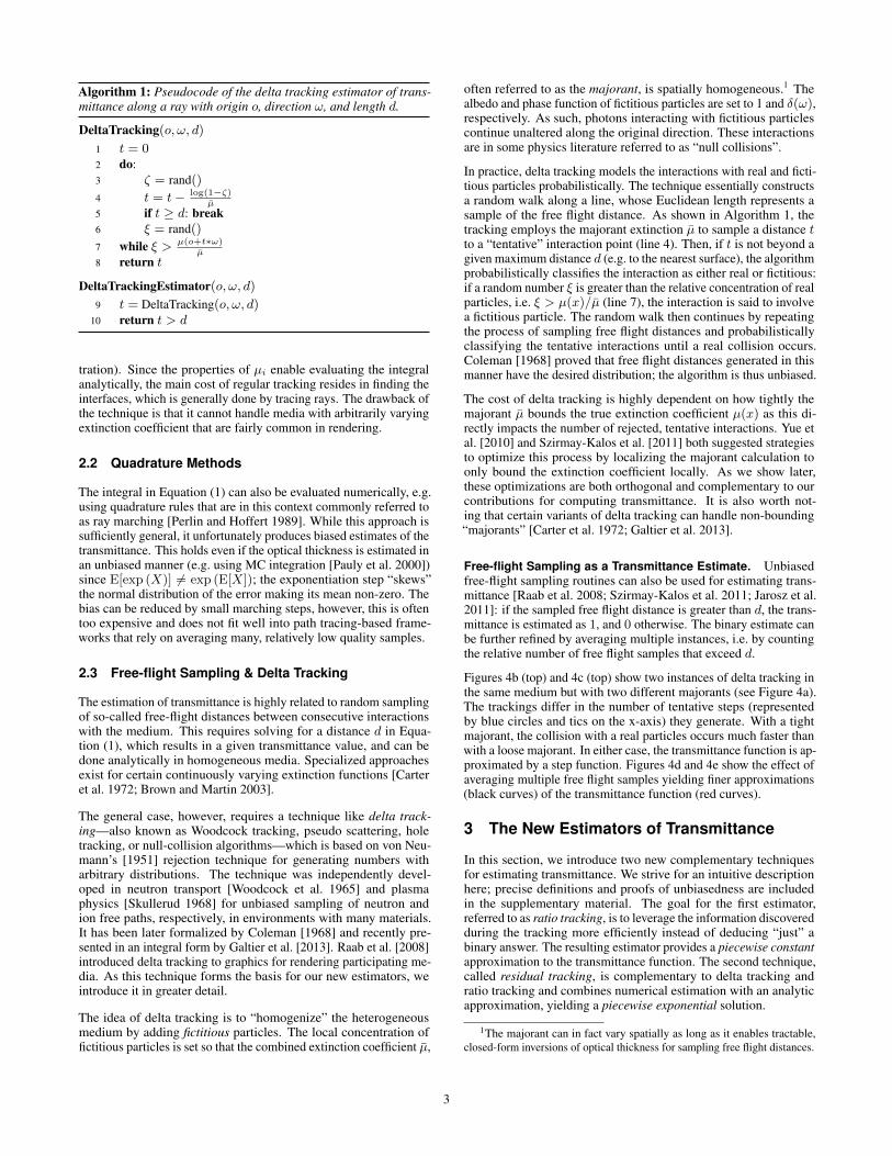
Algorithm 1: Pseudocode of the delta tracking estimator of trans-mittance along a ray with origin o, direction ω, and length d.

DeltaTracking(o, ω, d)

1 t = 02 do:3 ζ = rand()

4 t = t− log(1−ζ)µ

5 if t ≥ d: break6 ξ = rand()

7 while ξ > µ(o+t∗ω)µ

8 return t

DeltaTrackingEstimator(o, ω, d)

9 t = DeltaTracking(o, ω, d)10 return t > d

tration). Since the properties of µi enable evaluating the integralanalytically, the main cost of regular tracking resides in finding theinterfaces, which is generally done by tracing rays. The drawback ofthe technique is that it cannot handle media with arbitrarily varyingextinction coefficient that are fairly common in rendering.

2.2 Quadrature Methods

The integral in Equation (1) can also be evaluated numerically, e.g.using quadrature rules that are in this context commonly referred toas ray marching [Perlin and Hoffert 1989]. While this approach issufficiently general, it unfortunately produces biased estimates of thetransmittance. This holds even if the optical thickness is estimated inan unbiased manner (e.g. using MC integration [Pauly et al. 2000])since E[exp (X)] 6= exp (E[X]); the exponentiation step “skews”the normal distribution of the error making its mean non-zero. Thebias can be reduced by small marching steps, however, this is oftentoo expensive and does not fit well into path tracing-based frame-works that rely on averaging many, relatively low quality samples.

2.3 Free-flight Sampling & Delta Tracking

The estimation of transmittance is highly related to random samplingof so-called free-flight distances between consecutive interactionswith the medium. This requires solving for a distance d in Equa-tion (1), which results in a given transmittance value, and can bedone analytically in homogeneous media. Specialized approachesexist for certain continuously varying extinction functions [Carteret al. 1972; Brown and Martin 2003].

The general case, however, requires a technique like delta track-ing—also known as Woodcock tracking, pseudo scattering, holetracking, or null-collision algorithms—which is based on von Neu-mann’s [1951] rejection technique for generating numbers witharbitrary distributions. The technique was independently devel-oped in neutron transport [Woodcock et al. 1965] and plasmaphysics [Skullerud 1968] for unbiased sampling of neutron andion free paths, respectively, in environments with many materials.It has been later formalized by Coleman [1968] and recently pre-sented in an integral form by Galtier et al. [2013]. Raab et al. [2008]introduced delta tracking to graphics for rendering participating me-dia. As this technique forms the basis for our new estimators, weintroduce it in greater detail.

The idea of delta tracking is to “homogenize” the heterogeneousmedium by adding fictitious particles. The local concentration offictitious particles is set so that the combined extinction coefficient µ,

often referred to as the majorant, is spatially homogeneous.1 Thealbedo and phase function of fictitious particles are set to 1 and δ(ω),respectively. As such, photons interacting with fictitious particlescontinue unaltered along the original direction. These interactionsare in some physics literature referred to as “null collisions”.

In practice, delta tracking models the interactions with real and ficti-tious particles probabilistically. The technique essentially constructsa random walk along a line, whose Euclidean length represents asample of the free flight distance. As shown in Algorithm 1, thetracking employs the majorant extinction µ to sample a distance tto a “tentative” interaction point (line 4). Then, if t is not beyond agiven maximum distance d (e.g. to the nearest surface), the algorithmprobabilistically classifies the interaction as either real or fictitious:if a random number ξ is greater than the relative concentration of realparticles, i.e. ξ > µ(x)/µ (line 7), the interaction is said to involvea fictitious particle. The random walk then continues by repeatingthe process of sampling free flight distances and probabilisticallyclassifying the tentative interactions until a real collision occurs.Coleman [1968] proved that free flight distances generated in thismanner have the desired distribution; the algorithm is thus unbiased.

The cost of delta tracking is highly dependent on how tightly themajorant µ bounds the true extinction coefficient µ(x) as this di-rectly impacts the number of rejected, tentative interactions. Yue etal. [2010] and Szirmay-Kalos et al. [2011] both suggested strategiesto optimize this process by localizing the majorant calculation toonly bound the extinction coefficient locally. As we show later,these optimizations are both orthogonal and complementary to ourcontributions for computing transmittance. It is also worth not-ing that certain variants of delta tracking can handle non-bounding“majorants” [Carter et al. 1972; Galtier et al. 2013].

Free-flight Sampling as a Transmittance Estimate. Unbiasedfree-flight sampling routines can also be used for estimating trans-mittance [Raab et al. 2008; Szirmay-Kalos et al. 2011; Jarosz et al.2011]: if the sampled free flight distance is greater than d, the trans-mittance is estimated as 1, and 0 otherwise. The binary estimate canbe further refined by averaging multiple instances, i.e. by countingthe relative number of free flight samples that exceed d.

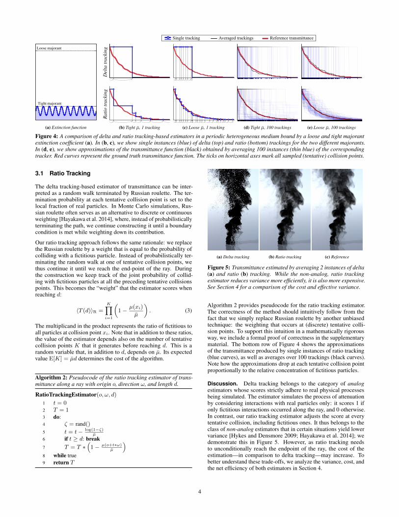
Figures 4b (top) and 4c (top) show two instances of delta tracking inthe same medium but with two different majorants (see Figure 4a).The trackings differ in the number of tentative steps (representedby blue circles and tics on the x-axis) they generate. With a tightmajorant, the collision with a real particles occurs much faster thanwith a loose majorant. In either case, the transmittance function is ap-proximated by a step function. Figures 4d and 4e show the effect ofaveraging multiple free flight samples yielding finer approximations(black curves) of the transmittance function (red curves).

3 The New Estimators of Transmittance

In this section, we introduce two new complementary techniquesfor estimating transmittance. We strive for an intuitive descriptionhere; precise definitions and proofs of unbiasedness are includedin the supplementary material. The goal for the first estimator,referred to as ratio tracking, is to leverage the information discoveredduring the tracking more efficiently instead of deducing “just” abinary answer. The resulting estimator provides a piecewise constantapproximation to the transmittance function. The second technique,called residual tracking, is complementary to delta tracking andratio tracking and combines numerical estimation with an analyticapproximation, yielding a piecewise exponential solution.

1The majorant can in fact vary spatially as long as it enables tractable,closed-form inversions of optical thickness for sampling free flight distances.

3

Single tracking Averaged trackings Reference transmittance

Tight majorant

Loose majorant

(a) Extinction function

Del

tatr

acki

ng

7.21

Rat

iotr

acki

ng

(b) Tight µ, 1 tracking (c) Loose µ, 1 tracking (d) Tight µ, 100 trackings (e) Loose µ, 100 trackings

Figure 4: A comparison of delta and ratio tracking-based estimators in a periodic heterogeneous medium bound by a loose and tight majorantextinction coefficient (a). In (b, c), we show single instances (blue) of delta (top) and ratio (bottom) trackings for the two different majorants.In (d, e), we show approximations of the transmittance function (black) obtained by averaging 100 instances (thin blue) of the correspondingtracker. Red curves represent the ground truth transmittance function. The ticks on horizontal axes mark all sampled (tentative) collision points.

3.1 Ratio Tracking

The delta tracking-based estimator of transmittance can be inter-preted as a random walk terminated by Russian roulette. The ter-mination probability at each tentative collision point is set to thelocal fraction of real particles. In Monte Carlo simulations, Rus-sian roulette often serves as an alternative to discrete or continuousweighting [Hayakawa et al. 2014], where, instead of probabilisticallyterminating the path, we continue constructing it until a boundarycondition is met while weighting down its contribution.

Our ratio tracking approach follows the same rationale: we replacethe Russian roulette by a weight that is equal to the probability ofcolliding with a fictitious particle. Instead of probabilistically ter-minating the random walk at one of tentative collision points, wethus continue it until we reach the end-point of the ray. Duringthe construction we keep track of the joint probability of collid-ing with fictitious particles at all the preceding tentative collisionspoints. This becomes the “weight” that the estimator scores whenreaching d:

〈T (d)〉R =

K∏i=1

(1− µ(xi)

µ

). (3)

The multiplicand in the product represents the ratio of fictitious toall particles at collision point xi. Note that in addition to these ratios,the value of the estimator depends also on the number of tentativecollision points K that it generates before reaching d. This is arandom variable that, in addition to d, depends on µ. Its expectedvalue E[K] = µd determines the cost of the algorithm.

Algorithm 2: Pseudocode of the ratio tracking estimator of trans-mittance along a ray with origin o, direction ω, and length d.

RatioTrackingEstimator(o, ω, d)

1 t = 02 T = 13 do:4 ζ = rand()

5 t = t− log(1−ζ)µ

6 if t ≥ d: break7 T = T ∗

(1− µ(o+t∗ω)

µ

)8 while true9 return T

(a) Delta tracking (b) Ratio tracking (c) Reference

Figure 5: Transmittance estimated by averaging 2 instances of delta(a) and ratio (b) tracking. While the non-analog, ratio trackingestimator reduces variance more efficiently, it is also more expensive.See Section 4 for a comparison of the cost and effective variance.

Algorithm 2 provides pseudocode for the ratio tracking estimator.The correctness of the method should intuitively follow from thefact that we simply replace Russian roulette by another unbiasedtechnique: the weighting that occurs at (discrete) tentative colli-sion points. To support this intuition in a mathematically rigorousway, we include a formal proof of correctness in the supplementarymaterial. The bottom row of Figure 4 shows the approximationsof the transmittance produced by single instances of ratio tracking(blue curves), as well as averages over 100 trackings (black curves).Note how the approximations drop at each tentative collision pointproportionally to the relative concentration of fictitious particles.

Discussion. Delta tracking belongs to the category of analogestimators whose scores strictly adhere to real physical processesbeing simulated. The estimator simulates the process of attenuationby considering interactions with real particles only: it scores 1 ifonly fictitious interactions occurred along the ray, and 0 otherwise.In contrast, our ratio tracking estimator adjusts the score at everytentative collision, including fictitious ones. It thus belongs to theclass of non-analog estimators that in certain situations yield lowervariance [Hykes and Densmore 2009; Hayakawa et al. 2014]; wedemonstrate this in Figure 5. However, as ratio tracking needsto unconditionally reach the endpoint of the ray, the cost of theestimation—in comparison to delta tracking—may increase. Tobetter understand these trade-offs, we analyze the variance, cost, andthe net efficiency of both estimators in Section 4.

4

Single tracking Reference transmittanceControl transmittance Averaged trackings (residual transmittance) Product

Med

ium

A

min

avg

max

extin

ctio

n co

effi

cien

t

distance.001

.01

.1

1

10

100

tran

smitt

ance

distance.001

.01

.1

1

10

100

tran

smitt

ance

distance.001

.01

.1

1

10

100

tran

smitt

ance

distance.001

.01

.1

1

10

100

tran

smitt

ance

distance

Med

ium

B

min

avg

max

extin

ctio

n co

effi

cien

t

distance

(a) Extinction function

.001

.01

.1

1

10

100

tran

smitt

ance

distance

(b) µc = µmin & delta tracking

.001

.01

.1

1

10

100

tran

smitt

ance

distance

(c) µc = µmin & ratio tracking

.001

.01

.1

1

10

100

tran

smitt

ance

distance

(d) µc = µavg & ratio tracking

.001

.01

.1

1

10

100

tran

smitt

ance

distance

(e) µc = µmax & ratio tracking

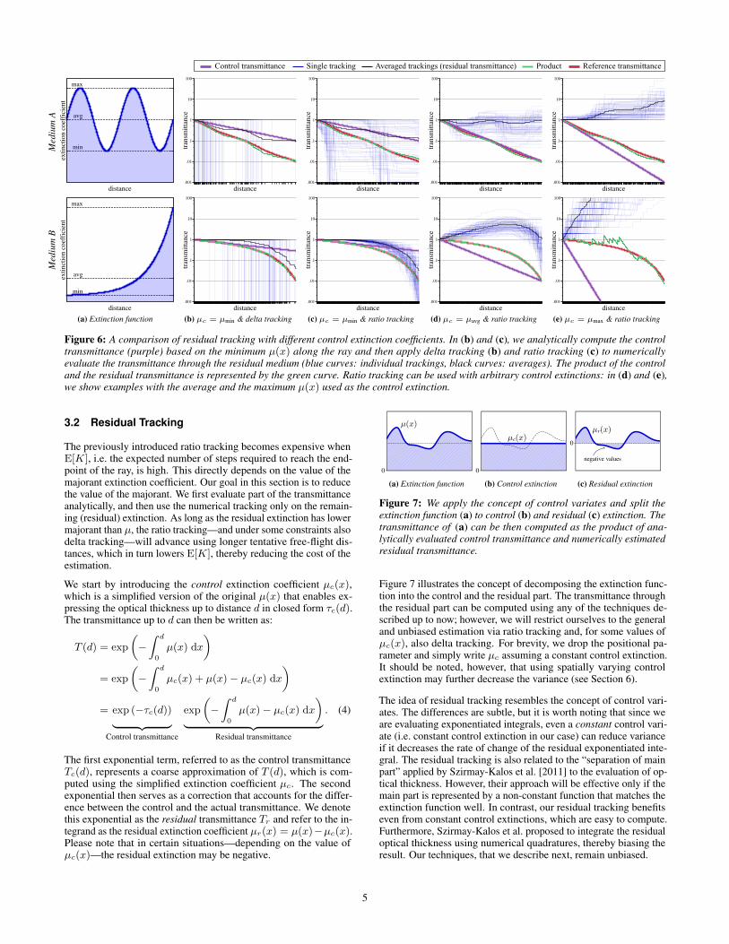
Figure 6: A comparison of residual tracking with different control extinction coefficients. In (b) and (c), we analytically compute the controltransmittance (purple) based on the minimum µ(x) along the ray and then apply delta tracking (b) and ratio tracking (c) to numericallyevaluate the transmittance through the residual medium (blue curves: individual trackings, black curves: averages). The product of the controland the residual transmittance is represented by the green curve. Ratio tracking can be used with arbitrary control extinctions: in (d) and (e),we show examples with the average and the maximum µ(x) used as the control extinction.

3.2 Residual Tracking

The previously introduced ratio tracking becomes expensive whenE[K], i.e. the expected number of steps required to reach the end-point of the ray, is high. This directly depends on the value of themajorant extinction coefficient. Our goal in this section is to reducethe value of the majorant. We first evaluate part of the transmittanceanalytically, and then use the numerical tracking only on the remain-ing (residual) extinction. As long as the residual extinction has lowermajorant than µ, the ratio tracking—and under some constraints alsodelta tracking—will advance using longer tentative free-flight dis-tances, which in turn lowers E[K], thereby reducing the cost of theestimation.

We start by introducing the control extinction coefficient µc(x),which is a simplified version of the original µ(x) that enables ex-pressing the optical thickness up to distance d in closed form τc(d).The transmittance up to d can then be written as:

T (d) = exp

(−∫ d

0

µ(x) dx

)= exp

(−∫ d

0

µc(x) + µ(x)− µc(x) dx

)= exp (−τc(d))︸︷︷︸

Control transmittance

exp

(−∫ d

0

µ(x)− µc(x) dx

)︸︷︷︸

Residual transmittance

. (4)

The first exponential term, referred to as the control transmittanceTc(d), represents a coarse approximation of T (d), which is com-puted using the simplified extinction coefficient µc. The secondexponential then serves as a correction that accounts for the differ-ence between the control and the actual transmittance. We denotethis exponential as the residual transmittance Tr and refer to the in-tegrand as the residual extinction coefficient µr(x) = µ(x)−µc(x).Please note that in certain situations—depending on the value ofµc(x)—the residual extinction may be negative.

(a) Extinction function (b) Control extinction (c) Residual extinction

Figure 7: We apply the concept of control variates and split theextinction function (a) to control (b) and residual (c) extinction. Thetransmittance of (a) can be then computed as the product of ana-lytically evaluated control transmittance and numerically estimatedresidual transmittance.

Figure 7 illustrates the concept of decomposing the extinction func-tion into the control and the residual part. The transmittance throughthe residual part can be computed using any of the techniques de-scribed up to now; however, we will restrict ourselves to the generaland unbiased estimation via ratio tracking and, for some values ofµc(x), also delta tracking. For brevity, we drop the positional pa-rameter and simply write µc assuming a constant control extinction.It should be noted, however, that using spatially varying controlextinction may further decrease the variance (see Section 6).

The idea of residual tracking resembles the concept of control vari-ates. The differences are subtle, but it is worth noting that since weare evaluating exponentiated integrals, even a constant control vari-ate (i.e. constant control extinction in our case) can reduce varianceif it decreases the rate of change of the residual exponentiated inte-gral. The residual tracking is also related to the “separation of mainpart” applied by Szirmay-Kalos et al. [2011] to the evaluation of op-tical thickness. However, their approach will be effective only if themain part is represented by a non-constant function that matches theextinction function well. In contrast, our residual tracking benefitseven from constant control extinctions, which are easy to compute.Furthermore, Szirmay-Kalos et al. proposed to integrate the residualoptical thickness using numerical quadratures, thereby biasing theresult. Our techniques, that we describe next, remain unbiased.

5

Min

imum

A ver

age

Max

imum

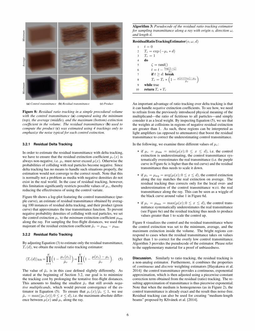
(a) Control transmittance (b) Residual transmittance (c) Product

Figure 8: Residual ratio tracking in a simple procedural volumewith the control transmittance (a) computed using the minimum(top), the average (middle), and the maximum (bottom) extinctioncoefficient in the volume. The residual transmittance (b) used tocompute the product (c) was estimated using 4 trackings only toemphasize the noise typical for each control extinction.

3.2.1 Residual Delta Tracking

In order to estimate the residual transmittance with delta tracking,we have to ensure that the residual extinction coefficient µr(x) isalways non-negative, i.e. µc must never exceed µ(x). Otherwise theprobabilities of colliding with real particles become negative. Sincedelta tracking has no means to handle such situations properly, theestimation would not converge to the correct result. Note that thisis normally not a problem as media with negative densities do notexist in the real world. In the case of residual tracking, however,this limitation significantly restricts possible values of µc, therebyreducing the effectiveness of using the control variate.

Figure 6b shows a log-plot featuring the control transmittance (pur-ple curve), an estimate of residual transmittance obtained by averag-ing 100 instances of residual delta tracking, and their product (greencurve) that approximates the true transmittance function. To preventnegative probability densities of colliding with real particles, we setthe control extinction µc to the minimum extinction coefficient µminalong the ray. For sampling the free-flight distances, we used themajorant of the residual extinction coefficient µr = µmax − µmin.

3.2.2 Residual Ratio Tracking

By adjusting Equation (3) to estimate only the residual transmittance,Tr(d), we obtain the residual ratio tracking estimator:

〈Tr(d)〉RR =

K∏i=1

(1− µr(xi)

µr

)=

K∏i=1

(1− µ(xi)− µc

µr

). (5)

The value of µr is in this case defined slightly differently. Asstated at the beginning of Section 3.2, our goal is to minimizethe tracking cost by prolonging the tentative free-flight distances.This amounts to finding the smallest µr that still avoids nega-tive multiplicands, which would prevent convergence of the es-timator in Equation (5). To ensure that µr(x)/µr ≤ 1, we useµr = max(|µr(x)|; 0 ≤ x ≤ d), i.e. the maximum absolute differ-ence between µ(x) and µc along the ray.

Algorithm 3: Pseudocode of the residual ratio tracking estimatorfor sampling transmittance along a ray with origin o, direction ω,and length d.

ResidualRatioTrackingEstimator(o, ω, d)

1 t = 02 Tc = exp (−µc ∗ d)3 Tr = 14 do5 ζ = rand()

6 t = t− log(1−ζ)µr

7 if t ≥ d: break8 Tr = Tr ∗

(1− µ(o+t∗ω)−µc

µr

)9 while true

10 return Tc ∗ Tr

An important advantage of ratio tracking over delta tracking is thatit can handle negative extinction coefficients. To see how, we needto refrain from the previously introduced physical meaning of themultiplicand—the ratio of fictitious to all particles—and simplyconsider it as a local weight. By inspecting Equation (5), we see thatthe weights at collisions in regions of negative residual extinctionare greater than 1. As such, these regions can be interpreted aslight amplifiers (as opposed to attenuators) that boost the residualtransmittance to correct the underestimating control transmittance.

In the following, we examine three different values of µc:

• if µc = µmin = min(µ(x); 0 ≤ x ≤ d), i.e. the controlextinction is underestimating, the control transmittance sys-tematically overestimates the real transmittance (i.e. the purplecurve in Figure 6c is higher than the red curve) and the residualtransmittance thus needs to scale it down.

• if µc = µavg = avg(µ(x); 0 ≤ x ≤ d), the control extinctionalong the ray matches the real extinction on average. Theresidual tracking thus corrects only for the local over- andunderestimation of the control transmittance w.r.t. the realtransmittance along the ray. This can be seen as a wiggle ofthe black curve around value 1 in Figure 6d.

• if µc = µmax = max(µ(x); 0 ≤ x ≤ d), the control trans-mittance systematically underestimates the real transmittance(see Figure 6e) and the residual tracking thus needs to producevalues greater than 1 to scale the control up.

Figure 8 visualizes the control and the residual transmittance wherethe control extinction was set to the minimum, average, and themaximum extinction inside the volume. The bright regions cor-respond to cases when the residual transmittance takes on valueshigher than 1 to correct for the overly low control transmittance.Algorithm 3 provides the pseudocode of the estimator. Please referto the supplementary material for a proof of unbiasedness.

Discussion. Similarly to ratio tracking, the residual tracking isa non-analog estimator. Furthermore, it combines the propertiesof continuous and discrete weighting estimators [Hayakawa et al.2014]: the control transmittance provides a continuous, exponentialapproximation, which is then adjusted using a piecewise-constantcorrection term obtained from the residual (ratio) tracking. The re-sulting approximation of transmittance is thus piecewise exponential.Note that when the medium is homogeneous (as in Figure 2), thecontrol transmittance is already exact and the result thus noise-free.Residual tracking can also be used for creating “medium-lengthbeams” proposed by Krivanek et al. [2014].

6

(a) Canonical scene

Rat

iotr

acki

ngD

elta

trac

king

0.1

0.2

0.3

0.4

0.5

0.6

0.7

0.8

0.9

0.01 0.10 1.00

colli

sion

sam

plin

g ef

fici

ency

extinction coefficient

0.1

0.2

0.3

0.4

0.5

0.6

0.7

0.8

0.9

0.01 0.10 1.00

colli

sion

sam

plin

g ef

fici

ency


(b) Equal cost render

0.1

0.2

0.3

0.4

0.5

0.6

0.7

0.8

0.9

0.01 0.10 1.00

colli

sion

sam

plin

g ef

fici

ency


0.1

0.2

0.3

0.4

0.5

0.6

0.7

0.8

0.9

0.01 0.10 1.00

colli

sion

sam

plin

g ef

fici

ency


(c) Variance (per instance)

0.1

0.2

0.3

0.4

0.5

0.6

0.7

0.8

0.9

0.01 0.10 1.00

colli

sion

sam

plin

g ef

fici

ency


0.1

0.2

0.3

0.4

0.5

0.6

0.7

0.8

0.9

0.01 0.10 1.00

colli

sion

sam

plin

g ef

fici

ency


(d) Cost (per instance)

0.1

0.2

0.3

0.4

0.5

0.6

0.7

0.8

0.9

0.01 0.10 1.00

colli

sion

sam

plin

g ef

fici

ency


0.1

0.2

0.3

0.4

0.5

0.6

0.7

0.8

0.9

0.01 0.10 1.00

colli

sion

sam

plin

g ef

fici

ency


(e) Product (c)×(d)

0.1

0.2

0.3

0.4

0.5

0.6

0.7

0.8

0.9

0.01 0.10 1.00

colli

sion

sam

plin

g ef

ficie

ncy


Delta tracking

Ratio tracking

color map

(f) Difference

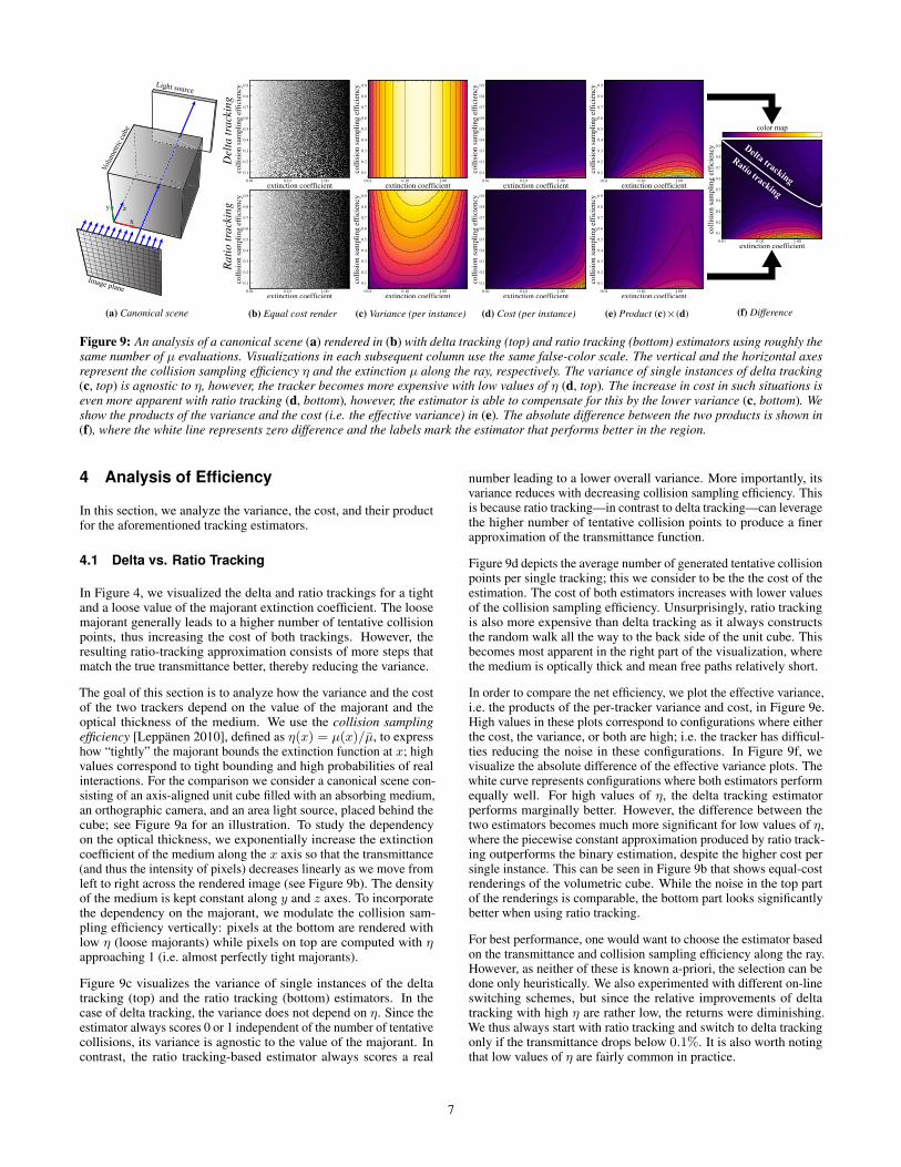
Figure 9: An analysis of a canonical scene (a) rendered in (b) with delta tracking (top) and ratio tracking (bottom) estimators using roughly thesame number of µ evaluations. Visualizations in each subsequent column use the same false-color scale. The vertical and the horizontal axesrepresent the collision sampling efficiency η and the extinction µ along the ray, respectively. The variance of single instances of delta tracking(c, top) is agnostic to η, however, the tracker becomes more expensive with low values of η (d, top). The increase in cost in such situations iseven more apparent with ratio tracking (d, bottom), however, the estimator is able to compensate for this by the lower variance (c, bottom). Weshow the products of the variance and the cost (i.e. the effective variance) in (e). The absolute difference between the two products is shown in(f), where the white line represents zero difference and the labels mark the estimator that performs better in the region.

4 Analysis of Efficiency

In this section, we analyze the variance, the cost, and their productfor the aforementioned tracking estimators.

4.1 Delta vs. Ratio Tracking

In Figure 4, we visualized the delta and ratio trackings for a tightand a loose value of the majorant extinction coefficient. The loosemajorant generally leads to a higher number of tentative collisionpoints, thus increasing the cost of both trackings. However, theresulting ratio-tracking approximation consists of more steps thatmatch the true transmittance better, thereby reducing the variance.

The goal of this section is to analyze how the variance and the costof the two trackers depend on the value of the majorant and theoptical thickness of the medium. We use the collision samplingefficiency [Leppanen 2010], defined as η(x) = µ(x)/µ, to expresshow “tightly” the majorant bounds the extinction function at x; highvalues correspond to tight bounding and high probabilities of realinteractions. For the comparison we consider a canonical scene con-sisting of an axis-aligned unit cube filled with an absorbing medium,an orthographic camera, and an area light source, placed behind thecube; see Figure 9a for an illustration. To study the dependencyon the optical thickness, we exponentially increase the extinctioncoefficient of the medium along the x axis so that the transmittance(and thus the intensity of pixels) decreases linearly as we move fromleft to right across the rendered image (see Figure 9b). The densityof the medium is kept constant along y and z axes. To incorporatethe dependency on the majorant, we modulate the collision sam-pling efficiency vertically: pixels at the bottom are rendered withlow η (loose majorants) while pixels on top are computed with ηapproaching 1 (i.e. almost perfectly tight majorants).

Figure 9c visualizes the variance of single instances of the deltatracking (top) and the ratio tracking (bottom) estimators. In thecase of delta tracking, the variance does not depend on η. Since theestimator always scores 0 or 1 independent of the number of tentativecollisions, its variance is agnostic to the value of the majorant. Incontrast, the ratio tracking-based estimator always scores a real

number leading to a lower overall variance. More importantly, itsvariance reduces with decreasing collision sampling efficiency. Thisis because ratio tracking—in contrast to delta tracking—can leveragethe higher number of tentative collision points to produce a finerapproximation of the transmittance function.

Figure 9d depicts the average number of generated tentative collisionpoints per single tracking; this we consider to be the the cost of theestimation. The cost of both estimators increases with lower valuesof the collision sampling efficiency. Unsurprisingly, ratio trackingis also more expensive than delta tracking as it always constructsthe random walk all the way to the back side of the unit cube. Thisbecomes most apparent in the right part of the visualization, wherethe medium is optically thick and mean free paths relatively short.

In order to compare the net efficiency, we plot the effective variance,i.e. the products of the per-tracker variance and cost, in Figure 9e.High values in these plots correspond to configurations where eitherthe cost, the variance, or both are high; i.e. the tracker has difficul-ties reducing the noise in these configurations. In Figure 9f, wevisualize the absolute difference of the effective variance plots. Thewhite curve represents configurations where both estimators performequally well. For high values of η, the delta tracking estimatorperforms marginally better. However, the difference between thetwo estimators becomes much more significant for low values of η,where the piecewise constant approximation produced by ratio track-ing outperforms the binary estimation, despite the higher cost persingle instance. This can be seen in Figure 9b that shows equal-costrenderings of the volumetric cube. While the noise in the top partof the renderings is comparable, the bottom part looks significantlybetter when using ratio tracking.

For best performance, one would want to choose the estimator basedon the transmittance and collision sampling efficiency along the ray.However, as neither of these is known a-priori, the selection can bedone only heuristically. We also experimented with different on-lineswitching schemes, but since the relative improvements of deltatracking with high η are rather low, the returns were diminishing.We thus always start with ratio tracking and switch to delta trackingonly if the transmittance drops below 0.1%. It is also worth notingthat low values of η are fairly common in practice.

7

min

avg

max

0 0.2 0.4 0.6 0.8 1

extin

ctio

n co

effi

cien

t

distance

min

avg

max

0.01 0.1 1

rela

tive

cont

rol e

xt. c

oef.


min

avg

max

0.01 0.1 1

rela

tive

cont

rol e

xt. c

oef.


min

avg

max

0.01 0.1 1

rela

tive

cont

rol e

xt. c

oef.


min

avg

max

0 0.2 0.4 0.6 0.8 1

extin

ctio

n co

effi

cien

t

distance

min

avg

max

0.01 0.1 1

rela

tive

cont

rol e

xt. c

oef.


min

avg

max

0.01 0.1 1

rela

tive

cont

rol e

xt. c

oef.


min

avg

max

0.01 0.1 1

rela

tive

cont

rol e

xt. c

oef.


min

avg

max

0 0.2 0.4 0.6 0.8 1

extin

ctio

n co

effi

cien

t

distance

min

avg

max

0.01 0.1 1

rela

tive

cont

rol e

xt. c

oef.


min

avg

max

0.01 0.1 1re

lativ

e co

ntro

l ext

. coe

f.extinction coefficient

min

avg

max

0.01 0.1 1

rela

tive

cont

rol e

xt. c

oef.

extinction coefficientmin

avg max

0 0.2 0.4 0.6 0.8 1

extin

ctio

n co

effi

cien

t

distancemin

avg max

0.1 1

rela

tive

cont

rol e

xt. c

oef.


avg max

0.1 1

rela

tive

cont

rol e

xt. c

oef.


avg max

0.1 1

rela

tive

cont

rol e

xt. c

oef.


(a) Extinction func. (b) Variance (c) Cost (d) Product (b)×(c) (e) Extinction func. (f) Variance (g) Cost (h) Product (f)×(g)

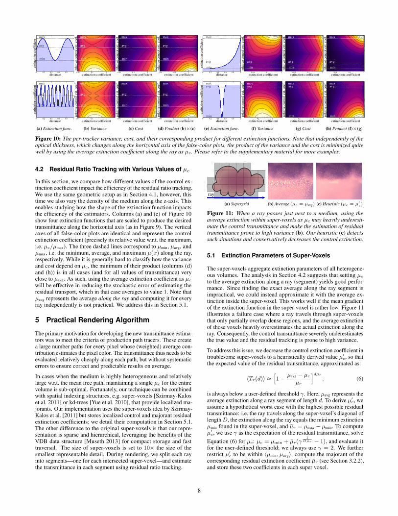
Figure 10: The per-tracker variance, cost, and their corresponding product for different extinction functions. Note that independently of theoptical thickness, which changes along the horizontal axis of the false-color plots, the product of the variance and the cost is minimized quitewell by using the average extinction coefficient along the ray as µc. Please refer to the supplementary material for more examples.

4.2 Residual Ratio Tracking with Various Values of µc

In this section, we compare how different values of the control ex-tinction coefficient impact the efficiency of the residual ratio tracking.We use the same geometric setup as in Section 4.1, however, thistime we also vary the density of the medium along the z-axis. Thisenables studying how the shape of the extinction function impactsthe efficiency of the estimators. Columns (a) and (e) of Figure 10show four extinction functions that are scaled to produce the desiredtransmittance along the horizontal axis (as in Figure 9). The verticalaxes of all false-color plots are identical and represent the controlextinction coefficient (precisely its relative value w.r.t. the maximum,i.e. µc/µmax). The three dashed lines correspond to µmin, µavg, andµmax, i.e. the minimum, average, and maximum µ(x) along the ray,respectively. While it is generally hard to classify how the varianceand cost depend on µc, the minimum of their product (columns (d)and (h)) is in all cases (and for all values of transmittance) veryclose to µavg. As such, using the average extinction coefficient as µcwill be effective in reducing the stochastic error of estimating theresidual transport, which in that case averages to value 1. Note thatµavg represents the average along the ray and computing it for everyray independently is not practical. We address this in Section 5.1.

5 Practical Rendering Algorithm

The primary motivation for developing the new transmittance estima-tors was to meet the criteria of production path tracers. These createa large number paths for every pixel whose (weighted) average con-tribution estimates the pixel color. The transmittance thus needs to beevaluated relatively cheaply along each path, but without systematicerrors to ensure correct and predictable results on average.

In cases when the medium is highly heterogeneous and relativelylarge w.r.t. the mean free path, maintaining a single µc for the entirevolume is sub-optimal. Fortunately, our technique can be combinedwith spatial indexing structures, e.g. super-voxels [Szirmay-Kaloset al. 2011] or kd-trees [Yue et al. 2010], that provide localized ma-jorants. Our implementation uses the super-voxels idea by Szirmay-Kalos et al. [2011] but stores localized control and majorant residualextinction coefficients; we detail their computation in Section 5.1.The other difference to the original super-voxels is that our repre-sentation is sparse and hierarchical, leveraging the benefits of theVDB data structure [Museth 2013] for compact storage and fasttraversal. The size of super-voxels is set to 10× the size of thesmallest representable detail. During rendering, we split each rayinto segments—one for each intersected super-voxel—and estimatethe transmittance in each segment using residual ratio tracking.

(a) Supergrid (b) Average (µc = µavg) (c) Heuristic (µc = µ′c)

Figure 11: When a ray passes just next to a medium, using theaverage extinction within super-voxels as µc may heavily underesti-mate the control transmittance and make the estimation of residualtransmittance prone to high variance (b). Our heuristic (c) detectssuch situations and conservatively decreases the control extinction.

5.1 Extinction Parameters of Super-Voxels

The super-voxels aggregate extinction parameters of all heterogene-ous volumes. The analysis in Section 4.2 suggests that setting µcto the average extinction along a ray (segment) yields good perfor-mance. Since finding the exact average along the ray segment isimpractical, we could instead approximate it with the average ex-tinction inside the super-voxel. This works well if the mean gradientof the extinction function in the super-voxel is rather low. Figure 11illustrates a failure case where a ray travels through super-voxelsthat only partially overlap dense regions, and the average extinctionof those voxels heavily overestimates the actual extinction along theray. Consequently, the control transmittance severely underestimatesthe true value and the residual tracking is prone to high variance.

To address this issue, we decrease the control extinction coefficient introublesome super-voxels to a heuristically derived value µ′c, so thatthe expected value of the residual transmittance, approximated as:

〈Tr(d)〉 ≈[1− µavg − µc

µr

]dµr, (6)

is always below a user-defined threshold γ. Here, µavg represents theaverage extinction along a ray segment of length d. To derive µ′c, weassume a hypothetical worst case with the highest possible residualtransmittance: i.e. the ray travels along the super-voxel’s diagonal oflengthD, the extinction along the ray equals the minimum extinctionµmin found in the super-voxel, and µr = µmax − µmin. To computeµ′c, we use γ as the expectation of the residual transmittance, solveEquation (6) for µc: µc = µmin + µr(γ

1Dµr − 1), and evaluate it

for the user-defined threshold; we always use γ = 2. We furtherrestrict µ′c to be within 〈µmin, µavg〉, compute the majorant of thecorresponding residual extinction coefficient µr (see Section 3.2.2),and store these two coefficients in each super voxel.

8

5.2 Rendering

In order to estimate the transmittance along a given ray, we performregular tracking through the super-voxel grid (i.e. 3D DDA [Ama-natides and Woo 1987]). For each intersected super-voxel, we iden-tify the overlapping ray segment and query the local µc and µr . Thetransmittance along the segment is computed by the product of con-trol transmittance and residual transmittance estimated using ratiotracking. The transmittance along the entire ray is then calculatedby multiplying the transmittances of all ray segments.

While performing the residual ratio tracking, we temporarily store afunctional representation of the transmittance along the entire ray.This is then used for constructing a numerical PDF for importancesampling the in-scattered light along the ray (our PDFs are propor-tional to the product of transmittance, scattering, and fluence), andfor estimating the transmittance to locations where we sample thein-scattered and/or emitted light.

6 Results

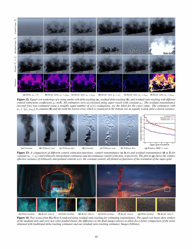
We implemented both estimators in the Mitsuba renderer [Jakob2010] and an in-house production renderer. Figure 12 shows unbi-ased renderings of a rising smoke plume—we purposely made itabsorptive to avoid variance due to scattering—computed by thetraditional delta tracking estimator, residual delta tracking estimator,and four variants of our residual ratio tracking estimator. The bottomrow visualizes the variance of each estimator. We use super-voxelsto store localized control and majorant extinction coefficients. Theresidual transmittance corrects only in regions where the controltransmittance underestimates or overestimates the true value. Tovisualize the noise, we use rather low per-pixel sample counts thatare adjusted to produce a roughly equal number of µ(x) evaluations;this in practice determines the performance of the algorithm.

While setting µc = µavg yields residual transport that is on averageclosest to 1 among all the tested variants, the product may sufferfrom high variance in configurations outlined in Section 5.1. Usingthe heuristically derived µ′c avoids these issues while preserving theRMSE obtained with µavg, which is about 2× lower than with thetraditional delta tracking-based estimator. A path tracer leveragingthe residual ratio tracking thus requires 4× fewer samples to resolvetransmittance at the quality obtained with delta tracking. It is worthnoting that not all values of µc reduce the error equally well, e.g.using µc = µmax yields significantly higher variance than µc = µmin.It is thus important to estimate the average extinction along the rayaccurately, or make µc rather underestimate the optimal value.

Figure 13 demonstrates the benefits of using trilinearly interpolatedcontrol extinction; we use the same polynomial approximation asSzirmay-Kalos et al. [2011] but apply it to µc instead of the majorant.Since the trilinearly interpolated control matches µ(x) better, theresidual transport does not deviate from 1 as much and can beestimated with lower variance. If we make the control extinctioncontinuous, e.g. by using the same µc for adjacent super-voxelcorners, the noise will change gradually over the image plane; thismay be in certain scenarios advantageous.

6.1 Media with Colored Extinction

Figure 1 shows a rendering obtained with our in-house productionrenderer. The clouds use “colored” extinction coefficients. Thisposes a problem for delta tracking, which, in order to preservehigh collision sampling efficiency, needs to handle the transmittancecomputation for each color channel independently. The estimationbecomes easier with our ratio tracking that maintains good effectiveperformance even with low values of η; all color channels can

thus be efficiently handled at once. For the control transmittance,we computed µc coefficients separately for each color and thenestimated the residual transmittance by a single instance of residualratio tracking, which uses the maximum µr across all color channels.

The insets emphasize the noise obtained with delta, ratio, and resid-ual ratio tracking with roughly the same number of µ(x) evaluations.In the top insets we disabled scattering to visualize the noise due tothe transmittance estimation only. As shown in the bottom insets,the different performance of the two estimators is clearly visibleeven when adding noisy estimates of multiple scattering; all render-ings use the same PDFs to sample in-scattering, the only differenceresides in the transmittance estimation. The residual ratio trackingyields lower RMSE producing results with roughly 6× lower effec-tive variance (i.e. the product of MSE and cost) when consideringjust the transmittance, and about 2.3× lower effective variance whensimulating multiple scattering in the medium. Figure 14 shows twomore examples with scattering media.

7 Discussion and Future Work

Overall Impact of Transmittance Estimation. Transmittance es-timation is only one of the many components of evaluating radiative-transport integrals. Here, we primarily focused on studying thevariance of transmittance estimators in isolation using metrics thatare renderer independent. In general, the reported improvementsshould lead to a corresponding decrease of noise in memory boundscenes where transmittance significantly impacts the quality.

Non-strict Majorants. The residual delta tracking and residualratio tracking estimators require strictly bounding majorants to avoidnegative probabilities or negative multiplicands, respectively. Carteret al. [1972] and Galtier et al. [2013] proposed weighted variantsof delta tracking that can deal with non-bounding majorants (i.e.negative densities of fictitious particles). These methods are quitepractical as they remove the burden of finding bounding majorants,be it at the cost of increased variance. While employing such weight-ing in residual delta tracking is trivial, applications to residual ratiotracking require careful variance analysis; we leave it as future work.

Free-flight Sampling. One could also leverage the concept ofcontrol variates and residual tracking for free-path sampling. As-suming that the control extinction represents a good approximationof µ(x) and the control optical thickness is invertible, free pathscould be sampled using the inversion method. The sample wouldthen be further weighted by the residual transmittance, which can beefficiently estimated for all channels via the residual ratio tracking.

Integral Formulation. We would like to note that ratio trackingcan be seen as a special case of the recently presented integralformulation of delta tracking [Galtier et al. 2013]. While we did notleverage this framework here, we believe it could offer a foundationfor deriving and proving new, weighted trackings, which may undercertain constraints be more efficient than the original algorithm.

8 Conclusion

We presented two complementary concepts that yield unbiased es-timators for efficient evaluation of transmittance in heterogeneousvolumes. In comparison to delta tracking, ratio tracking decreasesthe need for having tight majorants via improved efficiency in thosecases. When combined with the control transmittance, the residualratio tracking estimator gracefully handles media with low degree ofheterogeneity, simplifying to an analytic solution for homogeneous(sub)volumes. Furthermore, the estimators do not require any man-ual tuning (such as the step size in ray marching), and can be easily

9

Con

trol

tran

s.Tc

Res

idua

ltra

ns.Tr

Cost: 8.37MCost: 8.37MCost: 8.37MCost: 8.37MCost: 8.37MCost: 8.37MCost: 8.37MCost: 8.37MCost: 8.37MCost: 8.37MCost: 8.37MCost: 8.37MCost: 8.37MCost: 8.37MCost: 8.37MCost: 8.37MCost: 8.37M Cost: 8.07MCost: 8.07MCost: 8.07MCost: 8.07MCost: 8.07MCost: 8.07MCost: 8.07MCost: 8.07MCost: 8.07MCost: 8.07MCost: 8.07MCost: 8.07MCost: 8.07MCost: 8.07MCost: 8.07MCost: 8.07MCost: 8.07M Cost: 8.17MCost: 8.17MCost: 8.17MCost: 8.17MCost: 8.17MCost: 8.17MCost: 8.17MCost: 8.17MCost: 8.17MCost: 8.17MCost: 8.17MCost: 8.17MCost: 8.17MCost: 8.17MCost: 8.17MCost: 8.17MCost: 8.17M Cost: 8.17MCost: 8.17MCost: 8.17MCost: 8.17MCost: 8.17MCost: 8.17MCost: 8.17MCost: 8.17MCost: 8.17MCost: 8.17MCost: 8.17MCost: 8.17MCost: 8.17MCost: 8.17MCost: 8.17MCost: 8.17MCost: 8.17M Cost: 8.17MCost: 8.17MCost: 8.17MCost: 8.17MCost: 8.17MCost: 8.17MCost: 8.17MCost: 8.17MCost: 8.17MCost: 8.17MCost: 8.17MCost: 8.17MCost: 8.17MCost: 8.17MCost: 8.17MCost: 8.17MCost: 8.17M Cost: 8.17MCost: 8.17MCost: 8.17MCost: 8.17MCost: 8.17MCost: 8.17MCost: 8.17MCost: 8.17MCost: 8.17MCost: 8.17MCost: 8.17MCost: 8.17MCost: 8.17MCost: 8.17MCost: 8.17MCost: 8.17MCost: 8.17M

Pro

ductTc×Tr

RMSE: 0.026RMSE: 0.026RMSE: 0.026RMSE: 0.026RMSE: 0.026RMSE: 0.026RMSE: 0.026RMSE: 0.026RMSE: 0.026RMSE: 0.026RMSE: 0.026RMSE: 0.026RMSE: 0.026RMSE: 0.026RMSE: 0.026RMSE: 0.026RMSE: 0.026 RMSE: 0.024RMSE: 0.024RMSE: 0.024RMSE: 0.024RMSE: 0.024RMSE: 0.024RMSE: 0.024RMSE: 0.024RMSE: 0.024RMSE: 0.024RMSE: 0.024RMSE: 0.024RMSE: 0.024RMSE: 0.024RMSE: 0.024RMSE: 0.024RMSE: 0.024 RMSE: 0.022RMSE: 0.022RMSE: 0.022RMSE: 0.022RMSE: 0.022RMSE: 0.022RMSE: 0.022RMSE: 0.022RMSE: 0.022RMSE: 0.022RMSE: 0.022RMSE: 0.022RMSE: 0.022RMSE: 0.022RMSE: 0.022RMSE: 0.022RMSE: 0.022 RMSE: 0.012RMSE: 0.012RMSE: 0.012RMSE: 0.012RMSE: 0.012RMSE: 0.012RMSE: 0.012RMSE: 0.012RMSE: 0.012RMSE: 0.012RMSE: 0.012RMSE: 0.012RMSE: 0.012RMSE: 0.012RMSE: 0.012RMSE: 0.012RMSE: 0.012 RMSE: 0.012RMSE: 0.012RMSE: 0.012RMSE: 0.012RMSE: 0.012RMSE: 0.012RMSE: 0.012RMSE: 0.012RMSE: 0.012RMSE: 0.012RMSE: 0.012RMSE: 0.012RMSE: 0.012RMSE: 0.012RMSE: 0.012RMSE: 0.012RMSE: 0.012 RMSE: 0.049RMSE: 0.049RMSE: 0.049RMSE: 0.049RMSE: 0.049RMSE: 0.049RMSE: 0.049RMSE: 0.049RMSE: 0.049RMSE: 0.049RMSE: 0.049RMSE: 0.049RMSE: 0.049RMSE: 0.049RMSE: 0.049RMSE: 0.049RMSE: 0.049

V ari

ance

(a) Delta, µc=0 (b) Resid. delta, µc=µmin (c) Resid. ratio, µc=µmin (d) Resid. ratio, µc=µ′c (e) Resid. ratio, µc=µavg (f) Resid. ratio, µc=µmax

Figure 12: Equal-cost renderings of a rising smoke with delta tracking (a), residual delta tracking (b), and residual ratio tracking with differentcontrol extinctions coefficients µc (c-f). All estimators were accelerated using super-voxels with constant µc. The residual transmittance(second row) was estimated using a roughly equal number of µ(x) evaluations, see the label for the exact value. The estimators withµc ∈ {µ′c, µavg} in columns (d) and (e) yield the lowest error, which is visualized in the bottom row as equally scaled, false-colored variance.

(a) Constant (b) Trilinear cont. (c) Trilinear disc. (d) Constant (e) Trilinear cont. (f) Trilinear disc.

0

0.2

0.4

0.6

0.8

1

1.2

1.4

20 40 60 80 100 120

rela

tive

effe

ctiv

e va

rian

ce

super-grid resolution

ConstantTrilinear cont.Trilinear disc.

(g) Relative (MSE × cost)

Figure 13: A comparison of different control extinction functions: control transmittance (a, b, c) and residual transmittance (d, e, f) forconstant (µc = µ′c) and trilinearly interpolated continuous and discontinuous control extinction, respectively. The plot in (g) shows the relativeeffective variance of trilinearly interpolated controls w.r.t. the constant control; all plotted as functions of the resolution of the super-grid.

(a) Delta tracking (b) Resid. ratio tr. (c) Delta tracking (d) Resid. ratio tr. (e) Delta tracking (f) Resid. ratio tr. (g) Delta tracking (h) Resid. ratio tr.

Figure 14: Two scenes from Big Hero 6 rendered using residual ratio tracking for estimating transmittance. The equal-cost insets show rendersof the medium only and were not color graded (hence the difference to the final images above) to allow for a better comparison of the noiseobtained with traditional delta tracking estimator and our residual ratio tracking estimator. Images ©Disney.

10

combined with existing spatial indexing structures. Given that thecode changes w.r.t. delta tracking are minimal, integrating them intorenderers that already use delta tracking is trivial and well justifiedby the more effective handling of media with colored extinction.

9 Acknowledgments

We thank reviewers for their helpful comments, Simon Kallweit forimplementing the interpolated control extinction, and Oliver Klehmand Jaroslav Krivanek for proofreading. The bunny (Figure 2) andthe smoke (Figures 5, 13) are courtesy of the Stanford ComputerGraphics Laboratory and the OpenVDB library, respectively. Fig-ures 1 and 14 were rendered using Disney’s Hyperion Renderer.

References

AMANATIDES, J., AND WOO, A. 1987. A fast voxel traversalalgorithm for ray tracing. In Eurographics ’87, 3–10.

BROWN, F. B., AND MARTIN, W. R. 2003. Direct sampling ofMonte Carlo flight paths in media with continuously varyingcross-sections. In Proc. of ANS Mathematics & ComputationTopical Meeting, 6–11.

CARTER, L. L., CASHWELL, E. D., AND TAYLOR, W. M. 1972.Monte Carlo sampling with continuously varying cross sectionsalong flight paths. Nuclear Science and Engineering 48, 4, 403–411.

CEREZO, E., PEREZ, F., PUEYO, X., SERON, F. J., AND SILLION,F. X. 2005. A survey on participating media rendering techniques.The Visual Computer 21, 5, 303–328.

CHANDRASEKHAR, S. 1960. Radiative Transfer. Dover Publica-tions.

COLEMAN, W. A. 1968. Mathematical verification of a certainMonte Carlo sampling technique and applications of the techniqueto radiation transport problems. Nuclear Science and Engineering32, 1 (Apr.), 76–81.

DACHSBACHER, C., KRIVANEK, J., HASAN, M., ARBREE, A.,WALTER, B., AND NOVAK, J. 2013. Scalable realistic renderingwith many-light methods. Computer Graphics Forum 33, 1, 88–104.

GALTIER, M., BLANCO, S., CALIOT, C., COUSTET, C.,DAUCHET, J., HAFI, M. E., EYMET, V., FOURNIER, R., GAU-TRAIS, J., KHUONG, A., PIAUD, B., AND TERRE, G. 2013.Integral formulation of null-collision Monte Carlo algorithms.Journal of Quantitative Spectroscopy and Radiative Transfer 125(Apr.), 57–68.

GEORGIEV, I., KRIVANEK, J., HACHISUKA, T.,NOWROUZEZAHRAI, D., AND JAROSZ, W. 2013. Jointimportance sampling of low-order volumetric scattering. ACMTOG (Proc. of SIGGRAPH Asia) 32, 6 (Nov.), 164:1–164:14.

HAYAKAWA, C. K., SPANIER, J., AND VENUGOPALAN, V. 2014.Comparative analysis of discrete and continuous absorptionweighting estimators used in Monte Carlo simulations of radiativetransport in turbid media. J. Opt. Soc. Am. A 31, 2, 301–311.

HYKES, J. M., AND DENSMORE, J. D. 2009. Non-analog MonteCarlo estimators for radiation momentum deposition. Journalof Quantitative Spectroscopy and Radiative Transfer 110, 13,1097–1110.

JAKOB, W., 2010. Mitsuba renderer. http://www.mitsuba-renderer.org.

JAROSZ, W., NOWROUZEZAHRAI, D., THOMAS, R., SLOAN, P.-P., AND ZWICKER, M. 2011. Progressive photon beams. ACMTOG (Proc. of SIGGRAPH Asia) 30, 6 (Dec.), 181:1–181:12.

KAJIYA, J. T. 1986. The rendering equation. Computer Graphics(Proc. of SIGGRAPH), 143–150.

KELLER, A. 1997. Instant radiosity. In Proc. of SIGGRAPH97, ACM Press/Addison-Wesley Publishing Co., New York, NY,USA, Annual Conference Series, 49–56.

KULLA, C., AND FAJARDO, M. 2012. Importance samplingtechniques for path tracing in participating media. CGF (Proc. ofEurographics Symposium on Rendering) 31, 4 (June), 1519–1528.

KRIVANEK, J., GEORGIEV, I., HACHISUKA, T., VEVODA, P., SIK,M., NOWROUZEZAHRAI, D., AND JAROSZ, W. 2014. Unifyingpoints, beams, and paths in volumetric light transport simulation.ACM TOG (Proc. of SIGGRAPH) 33, 4, 103:1–103:13.

LAFORTUNE, E. P., AND WILLEMS, Y. D. 1993. Bi-directionalpath tracing. In Compugraphics ’93, 145–153.

LEPPANEN, J. 2010. Performance of Woodcock delta-tracking inlattice physics applications using the Serpent Monte Carlo reactorphysics burnup calculation code. Annals of Nuclear Energy 37, 5,715 – 722.

MUSETH, K. 2013. VDB: High-resolution sparse volumes withdynamic topology. ACM TOG 32, 3 (July), 27:1–27:22.

PAULY, M., KOLLIG, T., AND KELLER, A. 2000. Metropolislight transport for participating media. In Proc. of EurographicsWorkshop on Rendering Techniques, Springer-Verlag, London,UK, 11–22.

PERLIN, K. H., AND HOFFERT, E. M. 1989. Hypertexture. Com-puter Graphics (Proc. of SIGGRAPH) 23, 3 (July), 253–262.

PHARR, M., AND HUMPHREYS, G. 2010. Physically Based Render-ing: From Theory to Implementation, 2nd ed. Morgan KaufmannPublishers Inc., San Francisco, CA, USA.

RAAB, M., SEIBERT, D., AND KELLER, A. 2008. Unbiasedglobal illumination with participating media. In Monte Carlo andQuasi-Monte Carlo Methods 2006. Springer, 591–606.

SKULLERUD, H. R. 1968. The stochastic computer simulation ofion motion in a gas subjected to a constant electric field. Journalof Physics D: Applied Physics 1, 11, 1567–1568.

SZIRMAY-KALOS, L., TOTH, B., AND MAGDICS, M. 2011. Freepath sampling in high resolution inhomogeneous participatingmedia. Computer Graphics Forum 30, 1, 85–97.

VEACH, E., AND GUIBAS, L. J. 1994. Bidirectional estimators forlight transport. In Proc. of Eurographics Rendering Workshop1994, 147–162.

VON NEUMANN, J. 1951. Various techniques used in connectionwith random digits. Journal of Research of the National Bureauof Standards, Appl. Math. Series 12, 36–38.

WOODCOCK, E., MURPHY, T., HEMMINGS, P., AND T.C., L.1965. Techniques used in the GEM code for Monte Carlo neu-tronics calculations in reactors and other systems of complexgeometry. In Applications of Computing Methods to ReactorProblems, Argonne National Laboratory.

YUE, Y., IWASAKI, K., CHEN, B.-Y., DOBASHI, Y., ANDNISHITA, T. 2010. Unbiased, adaptive stochastic samplingfor rendering inhomogeneous participating media. ACM TOG(Proc. of SIGGRAPH Asia) 29, 6 (Dec.), 177:1–177:8.

11

Documents

Residual Ratio Tracking for Estimating Attenuation in