Embed Size (px)
Citation preview
8/11/2019 Attenuation Radiation
http://slidepdf.com/reader/full/attenuation-radiation 1/20
Attenuation of Radiation
by Dr. James E. Parks
Department of Physics and Astronomy401 Nielsen Physics Building
The University of Tennessee
Knoxville, Tennessee 37996-1200
Copyright © March, 2001 by James Edgar Parks*
*All rights are reserved. No part of this publication may be reproduced or transmitted in any form or by
any means, electronic or mechanical, including photocopy, recording, or any information storage or
retrieval system, without permission in writing from the author.
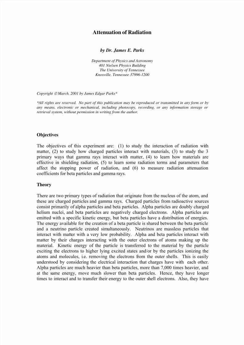
Objectives
The objectives of this experiment are: (1) to study the interaction of radiation with
matter, (2) to study how charged particles interact with materials, (3) to study the 3
primary ways that gamma rays interact with matter, (4) to learn how materials are
effective in shielding radiation, (5) to learn some radiation terms and parameters that
affect the stopping power of radiation, and (6) to measure radiation attenuation
coefficients for beta particles and gamma rays.
Theory
There are two primary types of radiation that originate from the nucleus of the atom, and
these are charged particles and gamma rays. Charged particles from radioactive sources
consist primarily of alpha particles and beta particles. Alpha particles are doubly charged
helium nuclei, and beta particles are negatively charged electrons. Alpha particles are
emitted with a specific kinetic energy, but beta particles have a distribution of energies.
The energy available for the creation of a beta particle is shared between the beta particle
and a neutrino particle created simultaneously. Neutrinos are massless particles that
interact with matter with a very low probability. Alpha and beta particles interact with
matter by their charges interacting with the outer electrons of atoms making up thematerial. Kinetic energy of the particle is transferred to the material by the particle
exciting the electrons to higher lying excited states and/or by the particles ionizing the
atoms and molecules, i.e. removing the electrons from the outer shells. This is easily
understood by considering the electrical interaction that charges have with each other.
Alpha particles are much heavier than beta particles, more than 7,000 times heavier, and
at the same energy, move much slower than beta particles. Hence, they have longer
times to interact and to transfer their energy to the outer shell electrons. Also, they have
8/11/2019 Attenuation Radiation
http://slidepdf.com/reader/full/attenuation-radiation 2/20
Attenuation of Radiation
twice the charge and the electrical interactions are therefore greater. As a result then,
alpha particles have greater interactions and give up their kinetic energy much more
quickly than do beta particles. Therefore, alpha particles have very short pathlengths in
the material. The range of charged particles at a given energy is defined as the average
distance they travel before they come to rest. The range of a 4 MeV alpha particle in air
is about 3 cm, and they can be stopped by a thin piece of paper or a thin sheet of someother solid or liquid material. 4 MeV beta particles have a maximum range of about
1,700 cm in air whereas they have a maximum range of about 2.0 cm in water and about
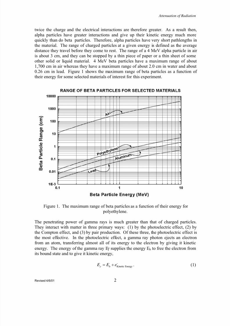
0.26 cm in lead. Figure 1 shows the maximum range of beta particles as a function of
their energy for some selected materials of interest for this experiment.
Figure 1. The maximum range of beta particles as a function of their energy for
polyethylene.
The penetrating power of gamma rays is much greater than that of charged particles.
They interact with matter in three primary ways: (1) by the photoelectric effect, (2) bythe Compton effect, and (3) by pair production. Of these three, the photoelectric effect is
the most effective. In the photoelectric effect, a gamma ray photon ejects an electron
from an atom, transferring almost all of its energy to the electron by giving it kinetic
energy. The energy of the gamma ray Eγ supplies the energy E b to free the electron from
its bound state and to give it kinetic energy,
. (1)-
Kinetic Energyb E E e
γ = +
Revised 4/6/01 2
8/11/2019 Attenuation Radiation
http://slidepdf.com/reader/full/attenuation-radiation 3/20
Attenuation of Radiation
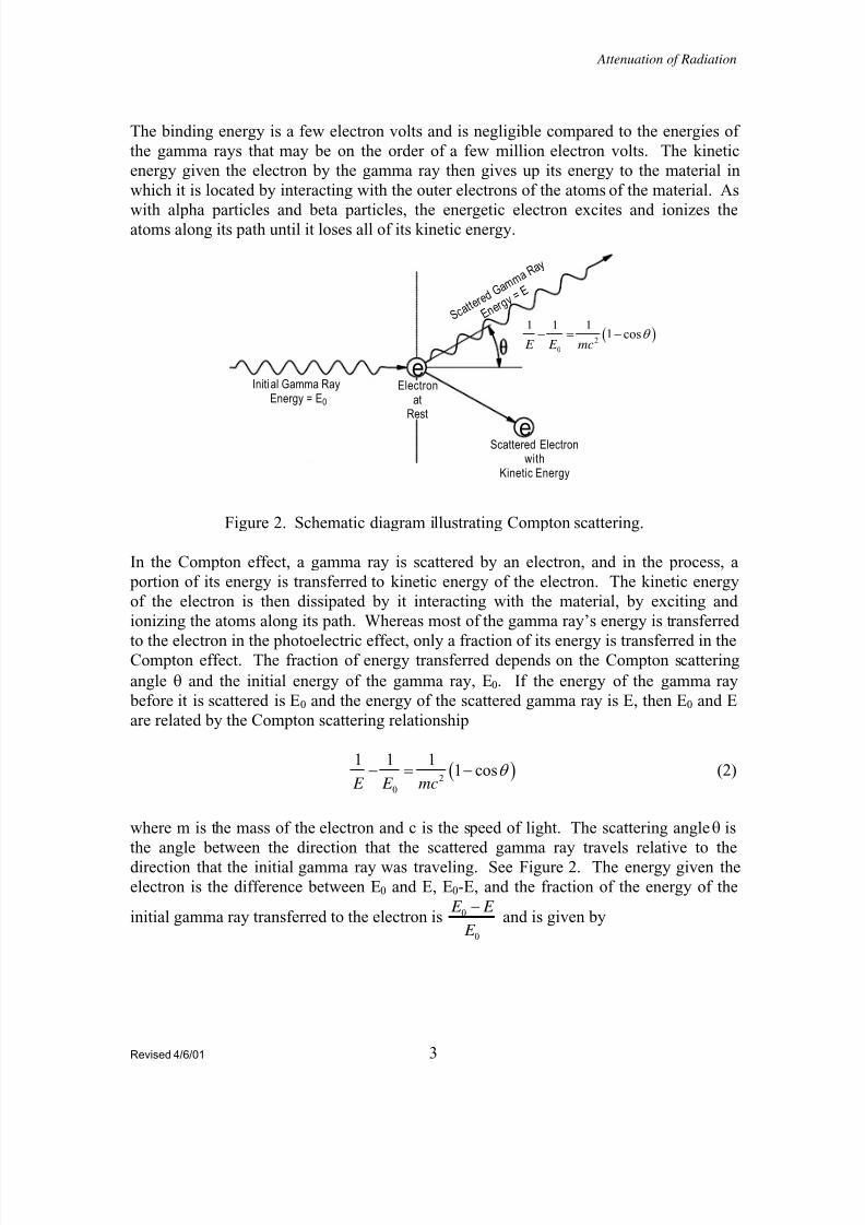
The binding energy is a few electron volts and is negligible compared to the energies of
the gamma rays that may be on the order of a few million electron volts. The kinetic
energy given the electron by the gamma ray then gives up its energy to the material in
which it is located by interacting with the outer electrons of the atoms of the material. As
with alpha particles and beta particles, the energetic electron excites and ionizes theatoms along its path until it loses all of its kinetic energy.
( )2
0
1 1 11 cos
E E mcθ − = −
e
e
Scattered Electronwith
Kinetic Energy
Initi al Gamma RayEnergy = E
S c a t t e
r e d G a m m
a R a y
E n e r g
y = E
Electronat
Rest0
Figure 2. Schematic diagram illustrating Compton scattering.
In the Compton effect, a gamma ray is scattered by an electron, and in the process, a
portion of its energy is transferred to kinetic energy of the electron. The kinetic energy
of the electron is then dissipated by it interacting with the material, by exciting and
ionizing the atoms along its path. Whereas most of the gamma ray’s energy is transferred
to the electron in the photoelectric effect, only a fraction of its energy is transferred in theCompton effect. The fraction of energy transferred depends on the Compton scattering
angle θ and the initial energy of the gamma ray, E0. If the energy of the gamma ray
before it is scattered is E0 and the energy of the scattered gamma ray is E, then E 0 and E
are related by the Compton scattering relationship
(2
0
1 1 11 cos
E E mc)θ − = − (2)
where m is the mass of the electron and c is the speed of light. The scattering angle θ is
the angle between the direction that the scattered gamma ray travels relative to the
direction that the initial gamma ray was traveling. See Figure 2. The energy given the
electron is the difference between E0 and E, E0-E, and the fraction of the energy of the
initial gamma ray transferred to the electron is 0
0
E E
E
− and is given by
Revised 4/6/01 3
8/11/2019 Attenuation Radiation
http://slidepdf.com/reader/full/attenuation-radiation 4/20
Attenuation of Radiation
( )
( )00
2
0 0
1 cos
1 cos
E E E
E mc E
θ
θ
⎡ ⎤−−= ⎢ ⎥
+ −⎣ ⎦. (3)
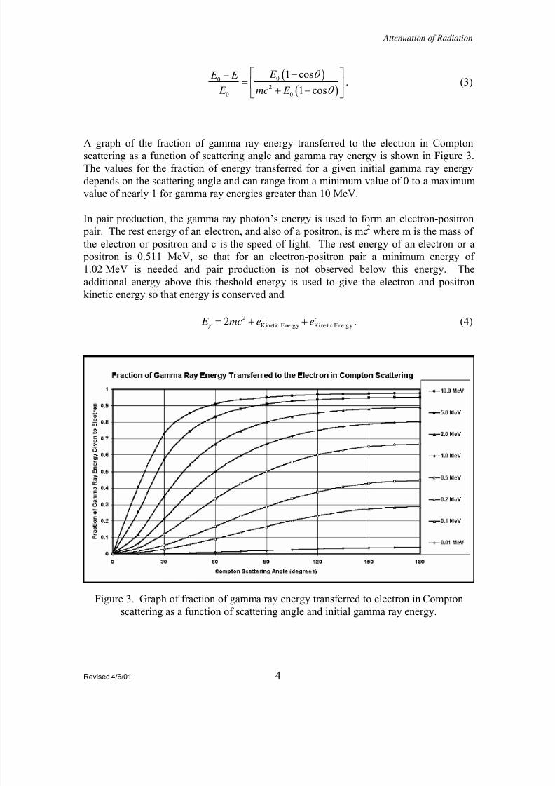
A graph of the fraction of gamma ray energy transferred to the electron in Compton
scattering as a function of scattering angle and gamma ray energy is shown in Figure 3.
The values for the fraction of energy transferred for a given initial gamma ray energy
depends on the scattering angle and can range from a minimum value of 0 to a maximum
value of nearly 1 for gamma ray energies greater than 10 MeV.
In pair production, the gamma ray photon’s energy is used to form an electron-positron
pair. The rest energy of an electron, and also of a positron, is mc2 where m is the mass of
the electron or positron and c is the speed of light. The rest energy of an electron or a
positron is 0.511 MeV, so that for an electron-positron pair a minimum energy of
1.02 MeV is needed and pair production is not observed below this energy. The
additional energy above this theshold energy is used to give the electron and positron
kinetic energy so that energy is conserved and
. (4)2 + -
Kinetic Energy Kinetic Energy2 E mc e eγ = + +
Figure 3. Graph of fraction of gamma ray energy transferred to electron in Compton
scattering as a function of scattering angle and initial gamma ray energy.
Revised 4/6/01 4
8/11/2019 Attenuation Radiation
http://slidepdf.com/reader/full/attenuation-radiation 5/20
Attenuation of Radiation
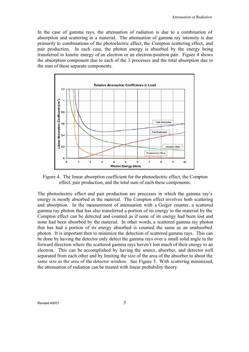
In the case of gamma rays, the attenuation of radiation is due to a combination of
absorption and scattering in a material. The attenuation of gamma ray intensity is due
primarily to combinations of the photoelectric effect, the Compton scattering effect, and
pair production. In each case, the photon energy is absorbed by the energy being
transferred to kinetic energy of an electron or an electron-positron pair. Figure 4 shows
the absorption component due to each of the 3 processes and the total absorption due tothe sum of these separate components.
Figure 4. The linear absorption coefficient for the photoelectric effect, the Compton
effect, pair production, and the total sum of each these components.
The photoelectric effect and pair production are processes in which the gamma ray’s
energy is mostly absorbed in the material. The Compton effect involves both scattering
and absorption. In the measurement of attenuation with a Geiger counter, a scattered
gamma ray photon that has also transferred a portion of its energy to the material by the
Compton effect can be detected and counted as if none of its energy had been lost and
none had been absorbed by the material. In other words, a scattered gamma ray photon
that has had a portion of its energy absorbed is counted the same as an unabsorbed
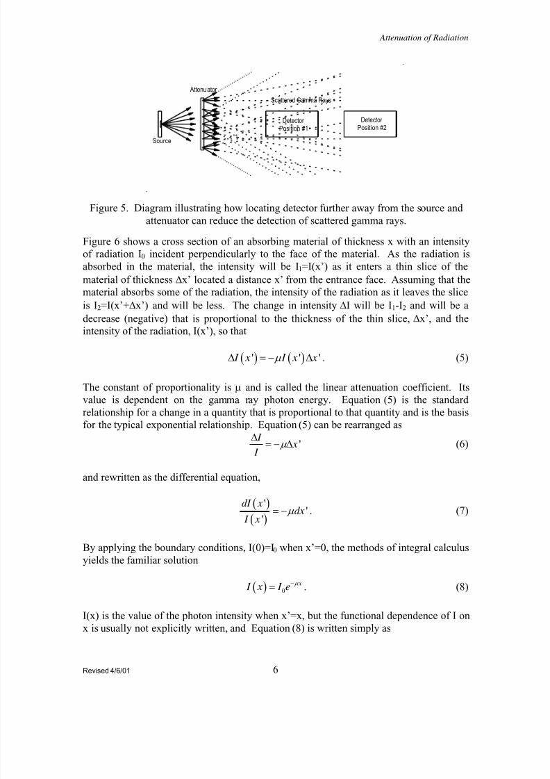
photon. It is important then to minimize the detection of scattered gamma rays. This can
be done by having the detector only detect the gamma rays over a small solid angle in the
forward direction where the scattered gamma rays haven’t lost much of their energy to anelectron. This can be accomplished by having the source, absorber, and detector well
separated from each other and by limiting the size of the area of the absorber to about the
same size as the area of the detector window. See Figure 5. With scattering minimized,
the attenuation of radiation can be treated with linear probability theory.
Revised 4/6/01 5
8/11/2019 Attenuation Radiation
http://slidepdf.com/reader/full/attenuation-radiation 6/20
Attenuation of Radiation
Detector Position #2
Detector Position #1
Source
Attenuator
Scattered Gamma Rays
Figure 5. Diagram illustrating how locating detector further away from the source and
attenuator can reduce the detection of scattered gamma rays.
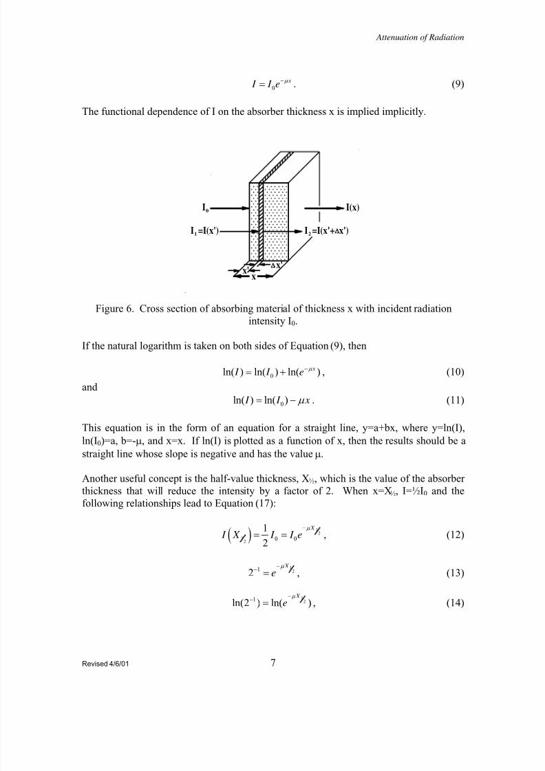
Figure 6 shows a cross section of an absorbing material of thickness x with an intensity
of radiation I0 incident perpendicularly to the face of the material. As the radiation is
absorbed in the material, the intensity will be I1=I(x’) as it enters a thin slice of the
material of thickness Δx’ located a distance x’ from the entrance face. Assuming that the
material absorbs some of the radiation, the intensity of the radiation as it leaves the slice
is I2=I(x’+Δx’) and will be less. The change in intensity ΔI will be I1-I2 and will be a
decrease (negative) that is proportional to the thickness of the thin slice, Δx’, and the
intensity of the radiation, I(x’), so that
( ) ( )' ' ' I x I xμ xΔ = − Δ . (5)
The constant of proportionality is μ and is called the linear attenuation coefficient. Its
value is dependent on the gamma ray photon energy. Equation (5) is the standard
relationship for a change in a quantity that is proportional to that quantity and is the basisfor the typical exponential relationship. Equation (5) can be rearranged as
' I
x I
μ Δ
= − Δ (6)
and rewritten as the differential equation,
( )
( )
''
'
dI xdx
I xμ = − . (7)
By applying the boundary conditions, I(0)=I0 when x’=0, the methods of integral calculusyields the familiar solution
( ) 0
x I x I e μ −= . (8)
I(x) is the value of the photon intensity when x’=x, but the functional dependence of I on
x is usually not explicitly written, and Equation (8) is written simply as
Revised 4/6/01 6
8/11/2019 Attenuation Radiation
http://slidepdf.com/reader/full/attenuation-radiation 7/20
Attenuation of Radiation
0
x I I e
μ −= . (9)
The functional dependence of I on the absorber thickness x is implied implicitly.
I =I(x') I =I(x'+ x')
I(x)I
1 2
0
x'x' x
+ + + + + ++++ + + + + + + +
+ + + + + +++
+ + + + + + + +
+ + + + + +++
+ + + + + + + +
+ + + + + ++++ + + + + + + +
+ + + + + +++
+ + + + + + + +
+ + + + + +++
+ + + + + + + +
+ + + + + ++++ + + + + + + +
+ + + + + +++
+ + + + + + + +
+ + + + + +++
+ + + + + + + +
+ + + + + +++
+ + + + + + + +
+ + + + + +++
+ + + + + + + +
+ + + + + +++
+ + + + + + + +
+ + + + + +++
+ + + + + + + +
Figure 6. Cross section of absorbing material of thickness x with incident radiation
intensity I0.
If the natural logarithm is taken on both sides of Equation (9), then
0ln( ) ln( ) ln( ) x I I e
μ −= + , (10)
and
0ln( ) ln( ) I I xμ = − . (11)
This equation is in the form of an equation for a straight line, y=a+bx, where y=ln(I),
ln(I0)=a, b=-μ, and x=x. If ln(I) is plotted as a function of x, then the results should be a
straight line whose slope is negative and has the value μ.
Another useful concept is the half-value thickness, X½, which is the value of the absorber
thickness that will reduce the intensity by a factor of 2. When x=X½, I=½I0 and the
following relationships lead to Equation (17):
( )
12
12 0 0
1
2
X
I X I I eμ −
= = , (12)
1212
X
eμ −− = , (13)
121
ln(2 ) ln( ) X
eμ −
− = , (14)
Revised 4/6/01 7
8/11/2019 Attenuation Radiation
http://slidepdf.com/reader/full/attenuation-radiation 8/20
Attenuation of Radiation
12
1ln(2) ln( ) X eμ − = − , (15)
12
ln(2) X μ = , (16)
and
1 12 2
ln(2) .693 X X
μ = = . (17)
Yet another useful concept is the mass attenuation coefficient μm where the thickness of a
slab of attenuator material is replaced by a new quantity called the mass thickness. If a
mass of material m has a uniform cross section A and length x, the volume density ρ is
defined as
m m
V A x
ρ = =
×
(18)
and the length x can be written as
1 1m
m x
A x
ρ ρ = × = × (19)
where xm is defined as the mass thickness. By substituting this value for x into Equation
(9) and by defining the mass attenuation coefficient as m
μ μ
ρ = a new relation,
1
0
m x I I e
ρ μ −
= (20)
is formed that yields
0m m x
I I e μ −= . (21)
The linear thickness is then measured in terms of the mass thickness in units of mass per
unit area (g/cm2, etc.) and the mass attenuation coefficient has the inverse units of
1/(mass/area) (1/gm/cm2). Just as Equation (9) could be written in the form of Equation
(11) by taking the natural logarithm of both sides, Equation (21) can be written as
0ln( ) ln( ) m m I I xμ = − . (22)
which is also in the form of an equation for a straight line, y=a+bx, where y=ln(I),
ln(I0)=a, b=-μm, and x=xm. If ln(I) is plotted as a function of xm, then the results should
be a straight line whose slope is negative and has the value of μm. The concept of a half-
value for mass thickness, Xm½, is the same as the concept for a half-value for linear
thickness. It is value of the mass thickness that will reduce the intensity by a factor of 2.
So when xm=Xm½, then I=½I0 and
Revised 4/6/01 8
8/11/2019 Attenuation Radiation
http://slidepdf.com/reader/full/attenuation-radiation 9/20
Attenuation of Radiation
( )1
21
20 0
1
2
m X
m I X I I e
μ −= = . (23)
Using the same mathematical operations that was used for the linear thickness,
1 12 2
ln(2) .693m
m m X X
μ = = (24)
and
12
.693m
m
X μ
= . (25)
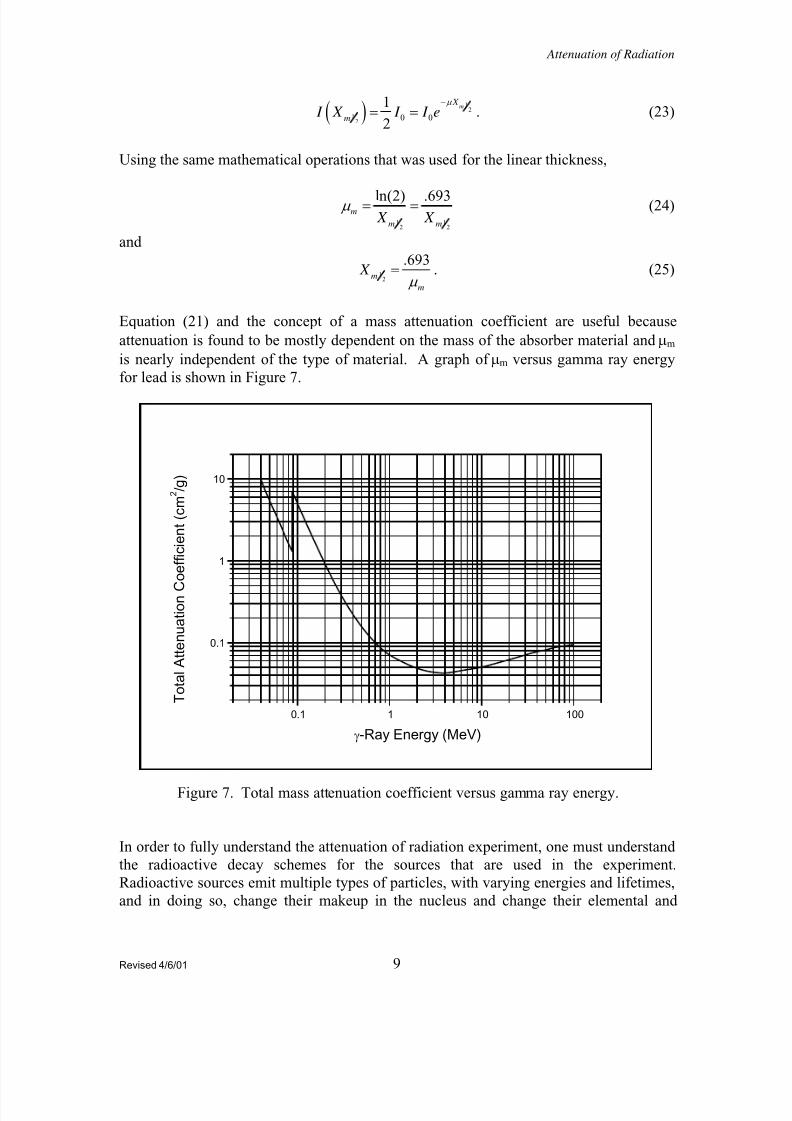
Equation (21) and the concept of a mass attenuation coefficient are useful because
attenuation is found to be mostly dependent on the mass of the absorber material and μm
is nearly independent of the type of material. A graph of μm versus gamma ray energy
for lead is shown in Figure 7.
0.1 1 10 100
0.1
1
10
T o t a l A t t e n u a t i o n C
o e f f i c i e n t ( c m
2 / g )
γ-Ray Energy (MeV)
Figure 7. Total mass attenuation coefficient versus gamma ray energy.
In order to fully understand the attenuation of radiation experiment, one must understand
the radioactive decay schemes for the sources that are used in the experiment.
Radioactive sources emit multiple types of particles, with varying energies and lifetimes,
and in doing so, change their makeup in the nucleus and change their elemental and
Revised 4/6/01 9
8/11/2019 Attenuation Radiation
http://slidepdf.com/reader/full/attenuation-radiation 10/20
Attenuation of Radiation
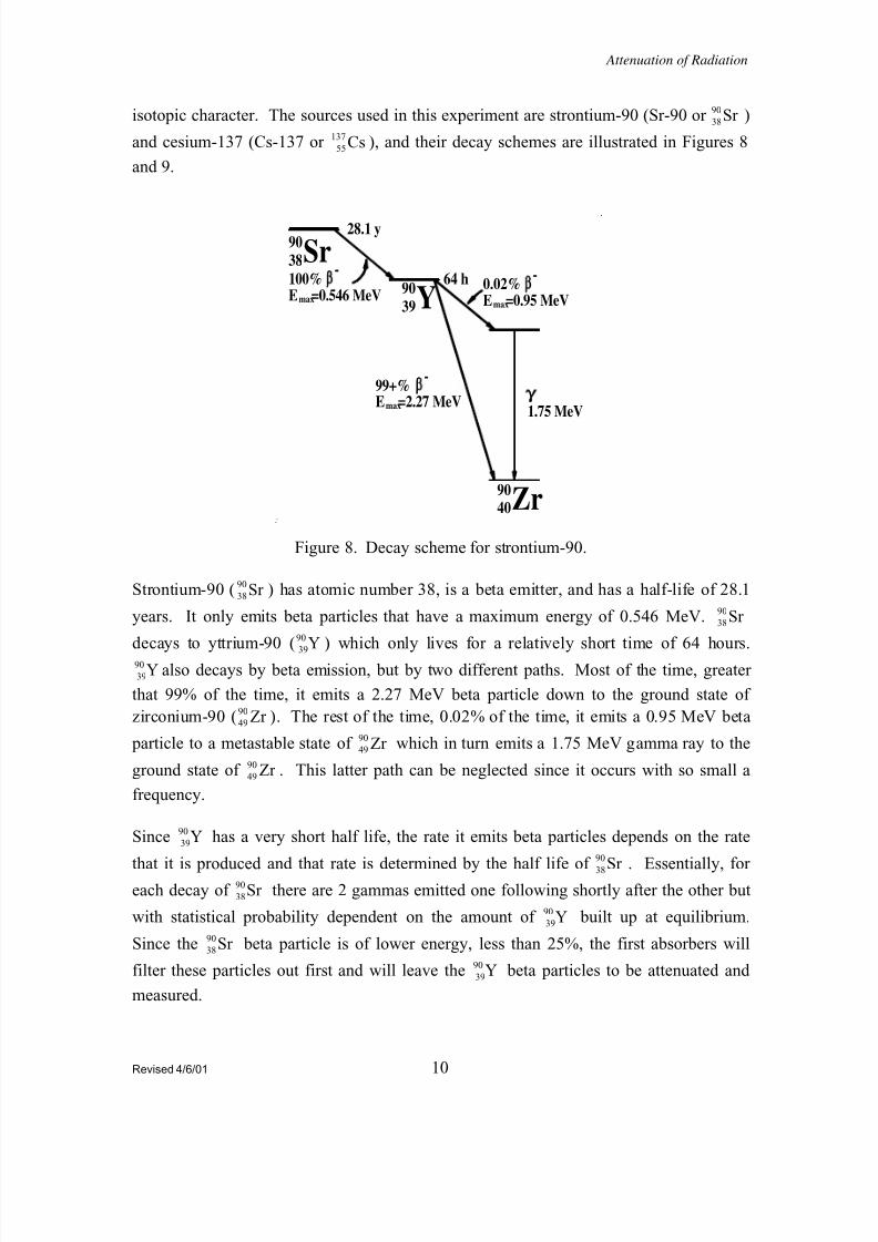
isotopic character. The sources used in this experiment are strontium-90 (Sr-90 or )
and cesium-137 (Cs-137 or 13 ), and their decay schemes are illustrated in Figures 8
and 9.
90
38Sr 7
55Cs
Y
Zr
Sr
39
40
38
90
90
90
64 h
28.1 y
99+%
0.02%100%
-
--
1.75 MeVE =2.27 MeV
E =0.95 MeVE =0.546 MeV
max
maxmax
Figure 8. Decay scheme for strontium-90.
Strontium-90 ( ) has atomic number 38, is a beta emitter, and has a half-life of 28.1
years. It only emits beta particles that have a maximum energy of 0.546 MeV.
decays to yttrium-90 ( ) which only lives for a relatively short time of 64 hours.
also decays by beta emission, but by two different paths. Most of the time, greater
that 99% of the time, it emits a 2.27 MeV beta particle down to the ground state of
zirconium-90 ( ). The rest of the time, 0.02% of the time, it emits a 0.95 MeV beta
particle to a metastable state of which in turn emits a 1.75 MeV gamma ray to the
ground state of . This latter path can be neglected since it occurs with so small a
frequency.
90
38Sr 90
38Sr 90
39
Y
90
39Y
90
49 Zr 90
49 Zr 90
49 Zr
Since has a very short half life, the rate it emits beta particles depends on the rate
that it is produced and that rate is determined by the half life of . Essentially, foreach decay of there are 2 gammas emitted one following shortly after the other but
with statistical probability dependent on the amount of built up at equilibrium.
Since the beta particle is of lower energy, less than 25%, the first absorbers will
filter these particles out first and will leave the beta particles to be attenuated and
measured.
90
39Y90
38Sr 90
38Sr 90
39Y90
38Sr 90
39Y
Revised 4/6/01 10
8/11/2019 Attenuation Radiation
http://slidepdf.com/reader/full/attenuation-radiation 11/20
Attenuation of Radiation
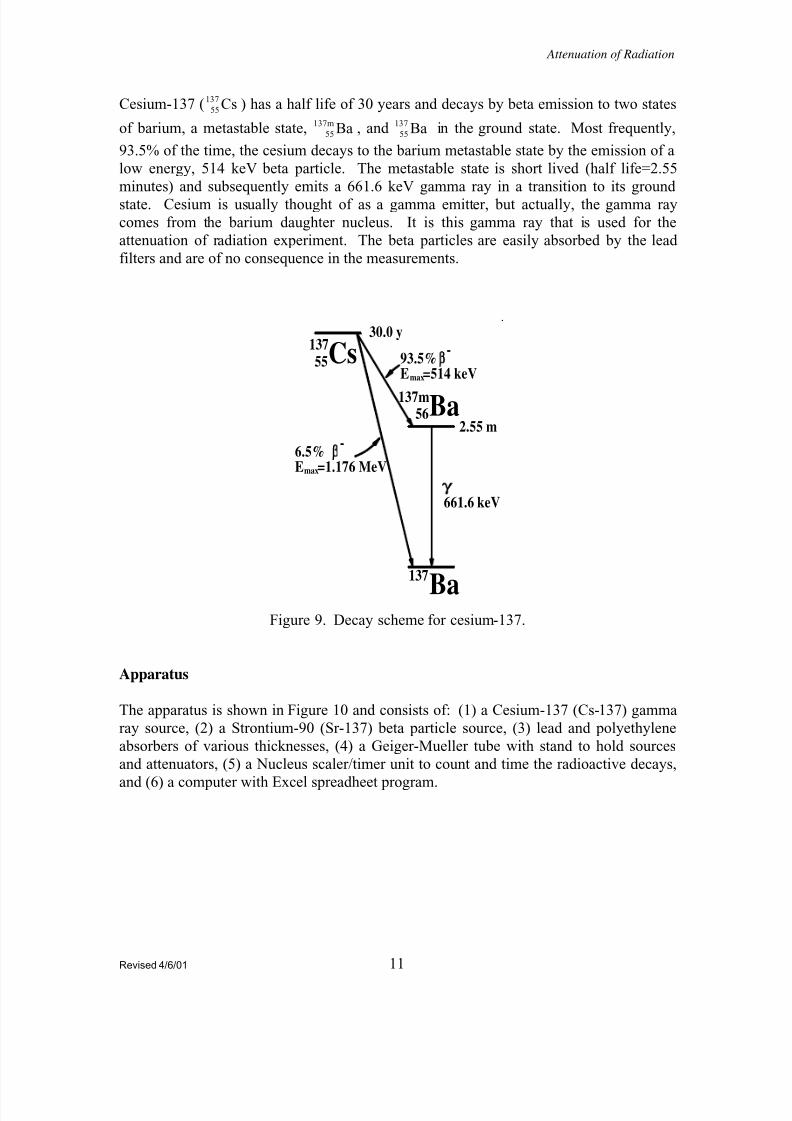
Cesium-137 ( 13 ) has a half life of 30 years and decays by beta emission to two states
of barium, a metastable state, , and 13 in the ground state. Most frequently,
93.5% of the time, the cesium decays to the barium metastable state by the emission of a
low energy, 514 keV beta particle. The metastable state is short lived (half life=2.55
minutes) and subsequently emits a 661.6 keV gamma ray in a transition to its ground
state. Cesium is usually thought of as a gamma emitter, but actually, the gamma ray
comes from the barium daughter nucleus. It is this gamma ray that is used for the
attenuation of radiation experiment. The beta particles are easily absorbed by the lead
filters and are of no consequence in the measurements.
7
55 Cs137m
55 Ba7
55 Ba
Ba
Ba
Cs
56
55
137m
137
137
2.55 m
30.0 y
6.5%
93.5%
-
-
661.6 keV
E =1.176 MeV
E =514 keV
max
max
Figure 9. Decay scheme for cesium-137.
Apparatus
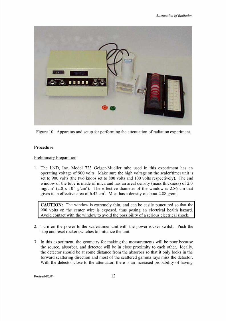
The apparatus is shown in Figure 10 and consists of: (1) a Cesium-137 (Cs-137) gamma
ray source, (2) a Strontium-90 (Sr-137) beta particle source, (3) lead and polyethylene
absorbers of various thicknesses, (4) a Geiger-Mueller tube with stand to hold sources
and attenuators, (5) a Nucleus scaler/timer unit to count and time the radioactive decays,
and (6) a computer with Excel spreadheet program.
Revised 4/6/01 11
8/11/2019 Attenuation Radiation
http://slidepdf.com/reader/full/attenuation-radiation 12/20
Attenuation of Radiation
Figure 10. Apparatus and setup for performing the attenuation of radiation experiment.
Procedure
Preliminary Preparation
1. The LND, Inc. Model 723 Geiger-Mueller tube used in this experiment has anoperating voltage of 900 volts. Make sure the high voltage on the scaler/timer unit is
set to 900 volts (the two knobs set to 800 volts and 100 volts respectively). The end
window of the tube is made of mica and has an areal density (mass thickness) of 2.0
mg/cm2 (2.0 x 10
-3 g/cm
2). The effective diameter of the window is 2.86 cm that
gives it an effective area of 6.42 cm2. Mica has a density of about 2.88 g/cm
3.
CAUTION: The window is extremely thin, and can be easily punctured so that the
900 volts on the center wire is exposed, thus posing an electrical health hazard.
Avoid contact with the window to avoid the possibility of a serious electrical shock.
2. Turn on the power to the scaler/timer unit with the power rocker switch. Push thestop and reset rocker switches to initialize the unit.
3. In this experiment, the geometry for making the measurements will be poor because
the source, absorber, and detector will be in close proximity to each other. Ideally,
the detector should be at some distance from the absorber so that it only looks in the
forward scattering direction and most of the scattered gamma rays miss the detector.
With the detector close to the attenuator, there is an increased probability of having
Revised 4/6/01 12
8/11/2019 Attenuation Radiation
http://slidepdf.com/reader/full/attenuation-radiation 13/20
Attenuation of Radiation
photons scatter from the edges of the absorber into the detector. Nevertheless, the
results should be very satisfactory and clearly demonstrate the principles.
4. In the first part of this experiment with the attenuation of gamma rays, the
measurements will be made by measuring the time for a fixed number of counts.
From Poisson Statistics for a large number of counts, the uncertainty in counts isequal to ± the square root of the average number of counts collected, i.e. N σ = ±
where σ is the uncertainty and N is the average number of counts. In the case here,
the number will be 5000 and the uncertainty will be 5000 71= . This represents an
uncertainty of71
100% 1.4%5000
× = and the measurements should be very good
statistically.
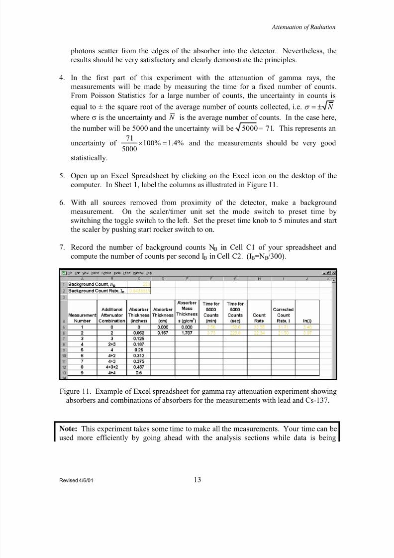
5. Open up an Excel Spreadsheet by clicking on the Excel icon on the desktop of the
computer. In Sheet 1, label the columns as illustrated in Figure 11.
6. With all sources removed from proximity of the detector, make a background
measurement. On the scaler/timer unit set the mode switch to preset time by
switching the toggle switch to the left. Set the preset time knob to 5 minutes and start
the scaler by pushing start rocker switch to on.
7. Record the number of background counts NB in Cell C1 of your spreadsheet and
compute the number of counts per second IB in Cell C2. (IB=NB/300).
Figure 11. Example of Excel spreadsheet for gamma ray attenuation experiment showingabsorbers and combinations of absorbers for the measurements with lead and Cs-137.
Note: This experiment takes some time to make all the measurements. Your time can be
used more efficiently by going ahead with the analysis sections while data is being
Revised 4/6/01 13
8/11/2019 Attenuation Radiation
http://slidepdf.com/reader/full/attenuation-radiation 14/20
Attenuation of Radiation
collected. The Excel spreadsheet program will automatically up-date the results as new
data are entered.
Attenuation of Gamma Rays
1. The procedure is to measure and record the count rate of detected gamma rays as a
function of the mass thickness of various absorbers that are placed between the
source and detector.
2. Obtain a Cs-137 source (orange disk) from the instructor and place it in the source
slide holder with the label side up. Place a #2 lead attenuator (0.062 inches, 1.80
g/cm2) on top of the source and slide holder to cover the source to absorb the beta
particles that are emitted as the cesium decays. Slide the source and source holder
with the #2 lead attenuator on top of the source into the fourth slot from the top of the
source/attenuator slide holder and detector stand. This combination of source and
attenuator will serve as the source to which additional attenuators will be added.
3. On the scaler/time unit set the mode switch to PRESET COUNT by switching the
toggle switch to the right. Set the PRESET COUNT knob to 5000 counts.
4. Start the counter with the start switch on the scaler. The scaler will measure and
display the time in minutes after it has collected 5000 counts and stopped. The
smallest time unit displayed is a hundredth of a minute, 0.01 minute. Record the time
in column F of your spreadsheet along with the values of the linear thickness and
mass thickness of the absorber used for the measurement in columns D and E. (For
this measurement, measurement #1, the thickness will be zero.)
5. Repeat the previous step by adding a second #2 absorber (0.062 inches thick) to a
second slide holder and insert it in the stand between the source and detector. Record
the time in column F, the linear thickness in columns D and the mass thickness in
column E of the spreadsheet.
6. Repeat these measurements until all the absorbers and combinations of absorbers
listed in the Excel spreadsheet in Figure 11 have been used. In each case record the
time to collect 5000 counts, the linear thickness, and the mass thickness of the lead in
the appropriate spreadsheet columns.
7. When completed, return the source to the front of the lab and to the instructor.Remove all the attenuators and place them in their proper locations in their storage
box.
Analysis of Results for the Attenuation of Gamma Rays
Revised 4/6/01 14
8/11/2019 Attenuation Radiation
http://slidepdf.com/reader/full/attenuation-radiation 15/20
Attenuation of Radiation
1. Make sure that the linear thickness and mass thickness is computed for each of the
absorbers and combinations of absorbers and recorded in columns D and E. Recall
that the mass thickness is just the normal thickness multiplied by the density of the
material. Lead has a density of 11.34 g/cm3 so that a 0.0625 inch thick lead absorber
has a normal thickness of 0.15875 cm and a mass thickness of 0.15875 cm x 11.34
g/cm3
=1.800 g/cm2
.
2. In column G compute the time in seconds from the times recorded in minutes in
column F. A formula, =F5*60 , can be entered in cell G5 and then copied down to
G13.
3. In column H compute the count rate for each of the measurements by dividing the
5000 counts detected by the time recorded in column G. A formula, =5000/G5, can
be entered in cell H5 and then copied down to H13.
4. In column I compute the corrected count rate by subtracting the background count
rate found in cell C2 from each on the count rates determined in column H. Aformula, =H5-$C$2, can be entered in cell I5 and then copied down to I13.
5. Since Equation (22) is the form of a linear equation and graphical analysis using
linear regression can be used to find the coefficients, use column J to compute the
natural logarithm of corrected count rates found in column I. A formula, =LN(I5), can be entered in cell J5 and then copied down to J13.
6. In the following steps, ln(I) will be graphed as a function of the mass thickness, xm.
According to the theory, the graph should result in a straight line whose slope is -μm.
All the points on the graph will seem to lie along a straight line, but if carefully
examined, the graph will appear to have two distinct linear portions, one with asteeper slope near the very beginning defined by the first 2 or 3 data points and a
second defined by the rest of the points. The linear portion with the first few points
and steeper slope is due to barium and lead x-rays. These are quickly filtered out
with the small attenuators and don’t contribute to the measurements with the thicker
absorbers. The graphical analysis will need to display this difference and the data for
the different portions will need to be analyzed separately. The slopes will be found
by linear regression using the trendline feature of Excel, but to do this, the data will
need to be broken into two components.
7. To graph all the points, choose Insert from the Excel main menu bar and then
Chart . . . from the pull down menu. Choose XY (Scatter) for the Chart type and the
points only option, , from Chart sub-type selections. Click on Next and then
click on the Series tab of the Chart Source Data window. Click the Add series button
and type All Points in the Name text input box. Type =Sheet1!$E$5:$E$13 in the XValues text input box and =Sheet1!$J$5:$J$13 in the Y Values text input box and
then click on Next.
Revised 4/6/01 15
8/11/2019 Attenuation Radiation
http://slidepdf.com/reader/full/attenuation-radiation 16/20
8/11/2019 Attenuation Radiation
http://slidepdf.com/reader/full/attenuation-radiation 17/20
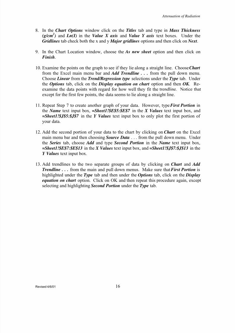
Attenuation of Radiation
Figure 12. Example graph of gamma ray attenuation by lead.
14. This graph should look something the one in Figure 12. The data ranges suggested
above for the first and second portions may not be consistent with your data. If not
you can edit the ranges by choosing Chart from the main menu and then
Source Data . . . .
15. The slope of the trendline for the second portion of the graph is negative and is equal
to -μm, the mass attenuation coefficient. Record the value of the slope taken from the
equation of the trendline in a convenient cell in sheet 1. Use another adjacent cell in
the same row or column to label this value.
16. By reading values from the graph in Figure 7 determine the value for the total mass
attenuation coefficient for 0.6616 MeV gamma rays and record this value in a cell
next to the slope value. Label an adjacent cell to identify the value.
17. Calculate the percent difference between the slope value and the graphical value, and
record this value properly labeled.
18. Examine the data in columns E and I and determine the mass thickness that reduces
the count rate by a factor of 2. From Equation (25) and your measured value for μm,
calculate the value of the half mass thickness, Xm½ and compare it to the value you
determined from the data. A plot of your data on semi-log graph paper and a linear
fit of the data would be a better way to determine this value since a table of numbers
is too discrete and a graph is continuous.
Attenuation of Beta Particles
Revised 4/6/01 17
8/11/2019 Attenuation Radiation
http://slidepdf.com/reader/full/attenuation-radiation 18/20
Attenuation of Radiation
1. Place the strontium-90 source (green disk) with its lettering topside in a source holder
tray and place it in the fifth slot (counting from the top slot) of the detector stand.
No attenuator will be placed on top of the source as in the previous case since beta
particles are the subject of this measurement.
2. In order to save time, these measurements will use a constant time period, and thecounting period will be set to 1 minute. The uncertainty between measurements will
change and will not be as good as the previous case, but the results will be acceptable
and the savings in time will be needed. Switch the scaler/timer unit’s toggle switch to
PRESET TIME and adjust the time period to 1 minute with the adjustment knobs.
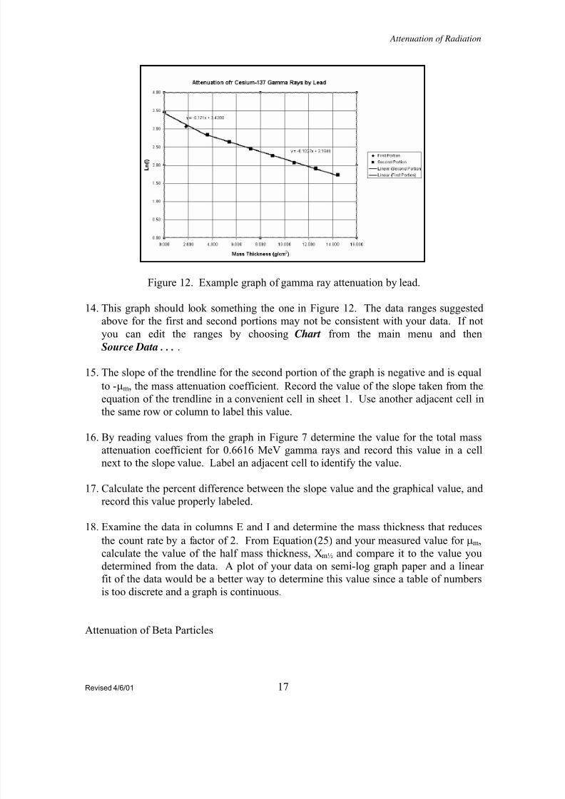
3. Open up Sheet 2 of your Excel workbook and label the columns as shown in
Figure 13. The absorbers to be used for the attenuation of betas are made of
polyethylene and are numbered. Figure 13 shows the attenuators and combinations of
attenuators to be used in the measurements, with the initial measurement having no
attenuator.
4. Enter the background count and background count rate from the previous experiment
since these values should not have changed.
5. Place the attenuator holder into the number 3 slot of the stand and make 1 minute
measurements of the beta particles for all the polyethylene attenuators and
combinations shown in Figure 13. Record your results in the appropriate column.
Figure 13. Example spreadsheet for recording and analyzing data for the attenuation of
beta particles by polyethylene.
6. Compute the mass thickness from the linear thickness, the count rate, the corrected
count rate, and the logarithm of the corrected count rate as was done in the gamma
ray absorption experiment. Polyethylene has a density of about 0.92 g/cm3 (920
mg/cm3) and is of much lower density than lead. It is more convenient to express the
Revised 4/6/01 18
8/11/2019 Attenuation Radiation
http://slidepdf.com/reader/full/attenuation-radiation 19/20
Attenuation of Radiation
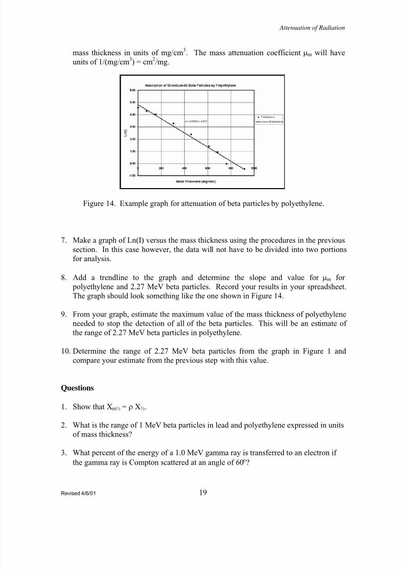
mass thickness in units of mg/cm3. The mass attenuation coefficient μm will have
units of 1/(mg/cm3) = cm
2/mg.
Figure 14. Example graph for attenuation of beta particles by polyethylene.
7. Make a graph of Ln(I) versus the mass thickness using the procedures in the previous
section. In this case however, the data will not have to be divided into two portions
for analysis.
8. Add a trendline to the graph and determine the slope and value for μm for
polyethylene and 2.27 MeV beta particles. Record your results in your spreadsheet.
The graph should look something like the one shown in Figure 14.
9. From your graph, estimate the maximum value of the mass thickness of polyethylene
needed to stop the detection of all of the beta particles. This will be an estimate of
the range of 2.27 MeV beta particles in polyethylene.
10. Determine the range of 2.27 MeV beta particles from the graph in Figure 1 and
compare your estimate from the previous step with this value.
Questions
1. Show that Xm½ = ρ X½.
2. What is the range of 1 MeV beta particles in lead and polyethylene expressed in units
of mass thickness?
3. What percent of the energy of a 1.0 MeV gamma ray is transferred to an electron if
the gamma ray is Compton scattered at an angle of 60°?
Revised 4/6/01 19
8/11/2019 Attenuation Radiation
http://slidepdf.com/reader/full/attenuation-radiation 20/20
Attenuation of Radiation
4. What are the 3 primary processes for the energy of a 3.5 MeV gamma ray to be
absorbed in lead and what is the relative effectiveness of each of these 3 processes in
transferring energy to the material?
5. What thickness of lead is needed to reduce the intensity of 1 MeV gamma rays to 1/8the initial intensity?
20