Resonance Entrainment of Tensegrity Structures via CPG Control · Resonance Entrainment of Tensegrity Structures via CPG Control Thomas K. Bliss a, Tetsuya Iwasaki b, Hilary Bart-Smith

Resonance Entrainment of Tensegrity

Structures via CPG Control

Thomas K. Bliss a, Tetsuya Iwasaki b, Hilary Bart-Smith a

aUniversity of Virginia, 122 Engineer’s Way, Charlottesville, VA 22903bUniversity of California, 420 Westwood Plaza, Los Angeles, CA 90095

Abstract

Neuronal circuits known as central pattern generators (CPG) are responsible forthe rhythmic motions in animal locomotion. These circuits exploit the resonantmodes of the body to produce efficient locomotion through sensory feedback. Assuch, the neuronal mechanisms are of interest in the control of autonomous roboticvehicles. The objective of this study is to establish a design framework that in-tegrates synthesized CPGs with tensegrity structures, with the goal of resonanceentrainment. Tensegrities are novel, nonlinear dynamic structures featuring highstrength to weight ratios, embedded actuation and sensing, and tunable stiffness.A two-neuron circuit known as a reciprocal inhibition oscillator is integrated withtensegrity structures with a pair of antagonistic actuators and collocated sensors.Each neuron has control of a cable length, and the sensory signal (current, stretchedlength) from the cable is fed back to the neuron. The frequency and amplitude ofclosed-loop oscillation are analyzed via harmonic balance, and a systematic methodfor control design is proposed to achieve entrainment to a prescribed resonancemode.

Key words: Neural control, Oscillation, Resonance, Harmonic balance, Tensegrity.

? Corresponding author T. K. Bliss. Tel. 434-982-4593. Fax 434-982-2037.Email addresses: [email protected] (Thomas K. Bliss), [email protected]

(Tetsuya Iwasaki), [email protected] (Hilary Bart-Smith).

Preprint submitted to Elsevier 10 August 2011

CONFIDENTIAL. Limited circulation. For review only

Preprint submitted to AutomaticaReceived August 11, 2011 05:40:50 PST

1 Introduction

Rhythmic motion in animals is ultimately controlled by central pattern gen-erators (CPGs), which are systems of neurons connected in such a way thattheir membrane potentials autonomously oscillate with particular phase rela-tionships between individual neurons. Brown [1] first illustrated that the CPGwas responsible for this behavior and suggested that sensory feedback servedto regulate the CPGs activity. He also cited reciprocal inhibition, where theactivity of antagonistic neurons inhibit each other, as a fundamental mecha-nism in rhythm generation. Pearce and Friesen [29] examined the contributionof sensory feedback, as well as peripheral neuronal and mechanical effects,to the coordination of rhythmic activity by comparing intact swimming ofmedicinal leeches and “fictive swimming” of isolated nerve chords. Friesen [5]then pointed out that reciprocal inhibition is responsible for oscillatory mo-tion in many species. He also showed that dynamic properties like synapticfatigue and impulse adaptation play an important role in oscillatory circuits.Ultimately, the literature illustrates that CPGs, consisting of neurons withreciprocal inhibition, are basic control units for rhythmic patterns. Sensoryfeedback has the ability to fine tune these patterns, resulting in coordinatedsignals essential to animal locomotion [6, 19, 28, 44].

These studies in biology have attracted the attention of engineers seeking ef-ficient control methodologies in robotics. Taga et al. [39] employed neuronalcircuits to control double pendulums modeling legs for bipedal locomotion, andobserved robust entrainment of the CPG to the mechanical system’s resonancefrequency. Williamson [43] used a CPG to control an arm with entrainmentto a hanging mass system, as well as turning a crank and ‘playing’ with aslinky. Kimura et al. [18] experimentally verified synthetic neuronal controlof a quadruped walking on irregular terrain as well as running on flat ter-rain using reflex signals to coordinate the CPG. Lewis and Bekey [20] andNakanishi et al. [27] also applied neuronal circuits to gait control and Lewis etal. [21] demonstrated the ability to create in silico CPGs. Chen and Iwasaki[3] developed a method for synthesizing oscillators with prescribed frequency,phase, and amplitude, and how to design such oscillators for feedback controlof an optimized locomotion variable.

Engineers have also investigated the mechanisms that provide entrainmentof neuronal circuits to a resonance of dynamic systems for efficient oscilla-tions [12, 43]. Verdaasdonk et al. [40, 41] simulated the neuro-musculo-skeletalsystem of the human arm, observing the conditions necessary for a reciprocalinhibition oscillator (RIO) to entrain to a resonance. Williams and DeWeerth[42] performed a case study of a simulated single degree of freedom (DOF)mass-spring-damper system controlled by an RIO, and commented on theform of feedback necessary for the RIO to entrain to the dynamic system

2



when the RIO’s intrinsic frequency is either above or below the resonanceof the mechanical system. Iwasaki and Zheng [15] compared the entrainmentof different RIO models to a pendulum, mapping the frequency against neu-ronal parameters. Then they used the method of harmonic balance to predictentrainment. Futakata and Iwasaki [9] formalized the graphical analysis in[15] and illustrated that negative integral feedback and positive rate feedbackare responsible for robust entrainment. All these studies focused on classicalstructures and models of one DOF systems like the pendulum and mass-spring-damper.

In the design of robotic locomotors, efficient propulsion can be achieved byexploiting a resonance. While CPGs appear to provide a fundamental controlframework for such applications, tensegrity structures are particularly suitablefor the mechanical part of the design due to their similarity to musculoskeletalsystems. Tensegrities are systems of bars held in compression with stabilityby a network of cables (or strings) in tension [32], where the bars and ca-bles can act like bones and muscles in biomechanical systems. The cables intensegrities provide a method of simultaneous actuation and sensing [22, 25],which is analogous to the biological motor control mechanism of regulatingmuscle stiffness through motoneuron activation and sensing the resulting mo-tion by stretch receptors. Originally developed by Snelson [34] and Fuller [7],tensegrities have attracted interest due to their high strength to weight ra-tios as well as their actuation capabilities [4, 37]. The statics [2, 24, 30] anddynamics [26, 31, 33] of tensegrities have been studied extensively. Their useas deployable antennae has been analyzed [8, 38], as well as controllable plat-forms for flight simulators [16, 35]. Despite various engineering applications oftensegrity structures, there seem to have been very few studies on tensegritiesin the context of morphing locomotors.

This paper develops a systematic method for designing a CPG-based feed-back controller that achieves entrainment to a resonance for a general class oftensegrity structures. We illustrate the potential of the tensegrity-CPG controlsystem for robotic applications, which has not been recognized in the control orrobotics communities. Coupling of neuronal control strategies with tensegritystructures provides a promising avenue for realization of morphing locomotorsinspired by biology. We will define a general class of multi-DOF tensegritystructures, and develop a method to design a CPG controller to achieve en-trainment to a prescribed resonance mode of oscillation. A single antagonisticpair of actuators is employed, where the formalization of the concept of anantagonistic actuator-sensor pair is a novel contribution. The design methodis based on harmonic balance [13] and hence an oscillation near a resonanceis to be achieved only approximately. The effectiveness of the proposed designmethod is illustrated by a three-cell tensegrity beam, which provides a basicplatform for robotic underwater vehicle applications.

3



2 Problem Formulation

This section formulates a control design problem. We consider the dynamics ofa general class of tensegrity structures for the plant, and develop the conceptof antagonistic actuation and sensing. The problem is to design a feedbackcontroller that achieves a closed-loop oscillation near a prescribed resonancemode. We adopt a control architecture based on a CPG as described below.

2.1 Tensegrity System

We consider a general tensegrity structure formed by multiple rigid bars con-nected by multiple flexible cables. The structure maintains a fixed shape atits nominal configuration through a static equilibrium of cable tensions. Theshape can be deformed through actuators that change the rest lengths of somecables. Let θ(t) ∈ Rn be a set of generalized coordinates representing theshape. For the ith cable, let li(t) be the current (stretched, deformed) lengthand λi(t) be the rest (original, undeformed) length. The cable is in tensionwhen li(t) > λi(t). We define the length vectors l(t), λ(t) ∈ Rm by stackingthe length values in columns, where m is the number of cables. The currentlength l(t) is uniquely determined by the current shape θ(t). The values ofthe variables at the equilibrium configuration are denoted by θe ∈ Rn andle, λe ∈ Rm.

Suppose the rest lengths of q cables are changed by actuators in real time. LetMa⊆ Im be the set of indices for the actuated cables, i.e., λi(t) for i ∈Ma arecontrolled by actuators, where Im is the set of positive integers up to m. Definethe control input by the rest length perturbation u(t) := Ta(λ(t)− λe), wherea positive input means that the cable is lengthened, and Ta ∈ Rq×m is a matrixformed by the ith rows of the identity matrix for i ∈Ma. For feedback controldesign, the current lengths of p cables, li(t) for i ∈Ms, are assumed available,where Ms ⊆ Im is the set of indices for sensed cables. Let Ts ∈ Rp×m be amatrix formed by the ith rows of the identity matrix for i ∈Ms, and define thesensor output as the current length perturbation y(t) := Ts(l(t)− le). A fullynonlinear model of the tensegrity system can be developed from the Euler-Lagrange equation. Assuming that the input u and the resulting perturbedmotion ϑ(t) := θ(t) − θe are both small, the input-output dynamics, from uto y, can be linearized and approximated by a p× q transfer function matrixP (s), as discussed in [36].

We assume that a point on the structure is fixed to the inertial frame, allthe bars are tightly constrained by the cable tensions at the equilibrium, andany admissible motions of the bars are subject to small friction. In this case,

4



there is no rigid body mode and the system is stable with lightly dampedpoles, which define n natural modes of oscillation. When the linear systemP (s) is driven by sinusoidal inputs u(t), the forced response y(t) has a locallymaximum amplitude at a resonance frequency, which is close to a naturalfrequency. The resonance and natural frequencies of the original nonlinearsystem would depend on the amplitude of oscillation in general, but are closeto those of the linear model when the amplitude is small.

2.2 Antagonistic Actuation and Collocated Sensing

We are interested in designing a feedback controller to achieve a prescribedmode of resonance oscillation for the closed-loop system (precise problem for-mulation will be given later). The first step toward this goal is to select cablesfor sensing and actuation. Tensegrity structures are analogous to musculoskele-tal systems in biology in that the cables act like muscles that actuate the body.An important property shared by cables and muscles is that they are only ableto impart force through tension, not compression. The property necessitatesat least a pair of antagonistic muscles to drive a skeletal joint in biologicalsystems. This motivates us to choose a pair of antagonistic cables to actuatethe tensegrity structure.

A nominal configuration of practical importance is one of symmetry, and thenatural oscillations about this configuration are symmetric as well. If twoactuators are placed at symmetric locations, then they would act as an antag-onistic pair. To elaborate on this point, consider a symmetric structure drivenby two symmetrically placed actuators with collocated sensors. In this case,the transfer function P (s) is 2 × 2, and let its (i, j)th entry be denoted byPij(s) with i, j = 1, 2. Since the effect of u1 on y2 is the same as that of u2 ony1 by symmetry, we have P12(s) = P21(s). By a similar argument, we arriveat P11(s) = P22(s). Hence, antagonistic actuations u1 = −u2 leads to

y1y2

=

P11 P12

P12 P11

u1

−u1

= (P11 − P12)

u1

−u1

,indicating that the resulting outputs y1 and y2 are also antagonistic; y1 = −y2.

For a general tensegrity structure, there may be no choice of antagonisticcables. The following is a definition for an extended notion of antagonicitythat broadens applicability of controlled tensegrity structures.

Definition 1 A system P (s) is said to be antagonistic if it has two inputs andtwo outputs, and there exist a nonzero scalar transfer function ρ(s), nonzero

5



η ∈ R, and matrices H,G ∈ R2×2 such that

HP (s)Ge = ηρ(s)e, ∀ s ∈ C, where e :=[

1 −1

]T. (1)

Condition (1) means that if a pair of anti-phase inputs u = e sin(ωt) is ap-plied to the augmented system HP (s)G, then its outputs oscillate also in ananti-phase manner in the steady state. The parameter η is redundant in thisdefinition but will become useful later as a design freedom. It turns out thatthe gain matrices H and G can always be chosen to be diagonal, providingconditioning of the inputs and outputs (i.e., scaling of their magnitudes) tothe original system P (s). Note that antagonicity of P (s) is equivalent to theexistence of matrices G and H such that HP (s)G has the fixed eigenvector efor all s ∈ C.

We consider a tensegrity structure described by an antagonistic transfer func-tion P (s). In addition, we assume that the sensors and actuators are collocated(Ma = Ms and Ta = Ts). It is well known that mechanical systems with col-located sensors and actuators are related to positive real transfer functions.For tensegrity structures, it can be proved that sensor/actuator collocationmakes sKP (s) positive real, where K is the diagonal matrix comprising thestiffnesses of the actuated cables (the slopes of the force-length curves at theequilibrium). An important consequence is that the transfer function ρ(s)in (1) can always be chosen such that sρ(s) is positive real for collocatedantagonistic systems.

In summary, we consider the class of systems satisfying the following:

Assumption 1 The system P (s) is stable with lightly damped poles, is an-tagonistic, and satisfies (1) with a positive real transfer function ρ(s).

A system is easily controllable to achieve high bandwidth tracking with a rea-sonable amount of control effort if the system is positive real [14]. Analogousto this fact, it turns out that the positive realness of the tensegrity system isimportant for achieving entrainment to the second or higher resonance mode.Selection of antagonistic actuators and collocated sensors is motivated by mus-culoskeletal biomechanics, and will make the RIO a particularly suitable choicefor the controller to achieve resonance entrainment as described in the nextsection.

2.3 CPG Control and Resonance Entrainment Problem

The most basic CPG unit is the reciprocal inhibition oscillator. It is a systemof two neurons with mutually inhibitory synaptic connections. Each neuron

6



can be modeled as a mapping from input wi to output vi as shown by [9]:

vi = ϕ(qi), qi = f(s)wi, f(s) :=2ωos

(s+ ωo)2, (2)

for i = 1, 2. The transfer function f(s) is a bandpass filter centered at thefrequency ωo, capturing the lag and adaptation characteristics of neuronaldynamics. The nonlinearity ϕ(x) captures the threshold property of neurons,and is assumed to be an odd, bounded, increasing function that is strictlyconcave on x > 0 and satisfies ϕ′(0) = ϕ(∞) = 1. A suitable choice for ϕ(x)is the hyperbolic tangent function, tanh(x), which is used in our numericalstudy.

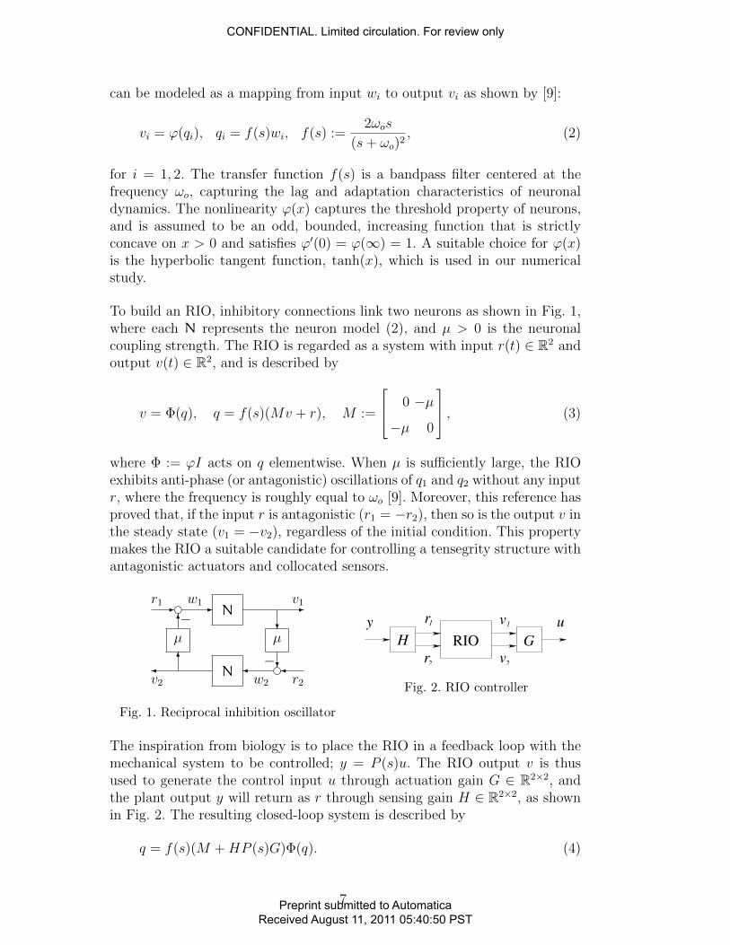
To build an RIO, inhibitory connections link two neurons as shown in Fig. 1,where each N represents the neuron model (2), and µ > 0 is the neuronalcoupling strength. The RIO is regarded as a system with input r(t) ∈ R2 andoutput v(t) ∈ R2, and is described by

v = Φ(q), q = f(s)(Mv + r), M :=

0 −µ

−µ 0

, (3)

where Φ := ϕI acts on q elementwise. When µ is sufficiently large, the RIOexhibits anti-phase (or antagonistic) oscillations of q1 and q2 without any inputr, where the frequency is roughly equal to ωo [9]. Moreover, this reference hasproved that, if the input r is antagonistic (r1 = −r2), then so is the output v inthe steady state (v1 = −v2), regardless of the initial condition. This propertymakes the RIO a suitable candidate for controlling a tensegrity structure withantagonistic actuators and collocated sensors.

e

eN

µ µ

N

-

?

?�6

6

- -

��

−

−

w1r1 v1

w2 r2v2

Fig. 1. Reciprocal inhibition oscillator

G

y r1

r2 v2

v1 u

RIOH

Fig. 2. RIO controller

The inspiration from biology is to place the RIO in a feedback loop with themechanical system to be controlled; y = P (s)u. The RIO output v is thusused to generate the control input u through actuation gain G ∈ R2×2, andthe plant output y will return as r through sensing gain H ∈ R2×2, as shownin Fig. 2. The resulting closed-loop system is described by

q = f(s)(M +HP (s)G)Φ(q). (4)

7



The symbols G and H are used for the gains here because it turns out thatgood choices for the gains are those satisfying the antagonicity condition (1).The problem addressed in this paper can now be formulated as follows.

Resonance Entrainment Problem: Consider the plant P (s) satisfyingAssumption 1 and the RIO control described by (3) and Fig. 2. Design thecontroller parameters G, H, µ, and ωo such that closed-loop oscillations for(4) occur at or close to a prescribed resonance mode.

It would be extremely difficult or intractable to solve the problem with theo-retical guarantees for existence and stability of a limit cycle or closeness to theresonance mode. To derive practically useful design conditions, we will chooseto address the problem through an approximate method in the next section.

The entrainment property has been fully analyzed and confirmed in a differentsetting (single-input, single-output one-DOF system) [9, 15]. We have adoptedthe RIO model in Fig. 1 from [9], but modified its input-output architecture todeal with two-input, two-output antagonistic systems arising from tensegritystructures. More importantly, the previous work dealt with a unique reso-nance of a one-DOF system, while we consider entrainment to one of manyresonance modes of a multi-DOF system, which is more difficult. A slightly dif-ferent control objective, called natural entrainment, has been considered formulti-DOF mechanical systems [10], where not only the frequency but alsothe mode shape are required to be close to a natural mode of oscillation. Acondition for natural entrainment of possibly underactuated systems is given,but this condition is strong due to the mode shape requirement and can oftenbe violated for systems with a small number of actuators (although it worksfine when fully actuated). Our problem formulation removes the mode shaperequirement, making it possible to obtain a more useful design condition forantagonistic systems.

3 Control Design for Resonance Entrainment

3.1 Design of Feedback Gains for Antagonicity

This section shows how to choose the feedback gains G and H. A reasonablechoice is those satisfying the antagonicity condition (1) because such choicewould make antagonistic oscillations of q1 and q2 a solution to the closed-loop system (4) as shown in the next section. The following result givesa computationally verifiable condition for checking whether a given transferfunction is antagonistic. The result also provides a constructive procedure tofind G and H.

8



Lemma 1 Let a stable 2×2 transfer function P (s) be given. The system P (s)is antagonistic if and only if Q is singular and R+RT is singular or indefinite,where Q and R are matrices constructed as follows. Let (A,B,C) be a minimalrealization of the transfer function

q(s) :=[P11(s) P12(s) P21(s) P22(s)

]T. (5)

Define Q := CXCT where X is the controllability Gramian of (A,B). For thenull space of Q, let r be its dimension, and let N ∈ R4×r be a matrix whosecolumns form its basis. Define R = n1n

T4 − n2n

T3, where ni ∈ Rr is the ith

column of NT.

Proof. There exists ρ(s) satisfying (1) if and only if

e⊥HP (s)Ge = 0 ⇔ hTP (s)g = 0,

⇔ tr(FP (s)) = 0,

⇔ q(s)Tf = 0,

where

e⊥ :=[1 1

], h := (e⊥H)T, g := Ge, F := ghT, f :=

[F11 F21 F12 F22

]T,

with Fij and Pij(s) being the (i, j) entries of F and P (s), respectively. Furthernote that, due to stability of q(s), we have

q(s)Tf = 0, ∀ s ∈ C ⇔ Qf = 0, Q :=1

2π

∫ ∞−∞

q(jω)q(jω)∗dω.

The matrix Q is given by Q = CXCT with the controllability Gramian X.Thus, existence of f such that Qf = 0 is necessary. Conversely, for such f ,the gain matrices G and H, such that F = ghT, can be constructed if andonly if det(F ) = 0, or f1f4 = f2f3 holds. Therefore, antagonicity is equivalentto the existence of a nonzero vector f such that Qf = 0 and f1f4 = f2f3. Avector f satisfies Qf = 0 if and only if f = Nz holds for some z ∈ Rr. Suchf satisfies f1f4 = f2f3 if and only if z is chosen to satisfy zTRz = 0. Finally,such nonzero z exists if and only if R +RT is indefinite or singular. 2

The definition and the associated verifiable condition for antagonicity can beapplied to any stable 2× 2 transfer function and are not limited to tensegritysystems. When the condition in Lemma 1 is satisfied, the parameters in (1)can be obtained as follows. First, let z ∈ Rr be a nonzero vector such thatzTRz = 0, and set f := Nz. Define F ∈ R2×2 by f = [ F11 F21 F12 F22 ]T.Let Go := diag(a1,−a2) and Ho := diag(b1, b2) be defined by any full rank

9



factor a, b ∈ R2 of F such that F = abT. Then the choice

G := gGo, H := hHo, η := gh, ρ(s) := eTHoP (s)Goe/2, (6)

satisfies (1) for arbitrary g, h ∈ R. The freedom in the sign of z can be used tointroduce normalization ρ(0) > 0 and make sρ(s) positive real when sensorsand actuators are collocated. For control design, we choose the feedback gainsG and H as described above, where Go and Ho are fixed but g and h are left asdesign parameters to be specified later. It turns out that the essential designfreedom is captured by their product η, and their individual values just scalethe oscillation amplitude of the tensegrity structure.

3.2 Oscillation Analysis

In this section, we show that the choice of feedback gains made in the previoussection leads to a closed-loop system that can have antagonistic oscillationswhen the controller parameters η, µ, and ωo are chosen appropriately. Wewill apply the method of harmonic balance [13] to the closed-loop systemand derive a condition under which the harmonic balance predicts existenceof oscillations. The frequency and amplitude of oscillation are also character-ized. The result will be used in the subsequent sections to examine when thepredicted frequency is close to one of the resonance frequencies.

The set of solutions q(t) to the closed-loop system (4), with G and H satisfying(1), includes antagonistic trajectories characterized by q(t) = x(t)e for somescalar signal x(t). To see this, note that e is an eigenvector of both M andHP (s)G:

Me = µe, HP (s)Ge = ηρ(s)e.

Hence, the signal q(t) = x(t)e satisfies (4), where x(t) is a solution to

x = f(s)(µ+ ηρ(s))ϕ(x). (7)

Thus, if this system has a periodic trajectory x(t), then the closed-loop system(4) has antagonistic oscillations q(t) = x(t)e. The design parameters in (7) areµ, η, and ωo embedded in f(s).

We analyze the system (7) using describing functions [17]. Recall that a pe-riodic signal x(t) may be approximated by a sinusoid x(t) ∼= a sin(ωt + b)through the Fourier series expansion. Such approximation would be reason-able for (7) because the band pass filter f(s) attenuates the bias and higherorder harmonics. The describing function of the nonlinearity ϕ(·) is an ampli-tude dependent gain κ(a) such that ϕ(x) ∼= κ(a)x, where the approximation

10



is based on the Fourier series of ϕ(x). When ϕ is an odd sigmoid function asassumed earlier, κ(a) is real valued and monotonically decreasing from one tozero on a > 0.

Approximating the nonlinearity ϕ(x) by its describing function κ(a)x, thesystem (7) becomes quasi-linear and its characteristic equation is given by

1 = ηκ(a)f(s)g(s), g(s) := µ/η + ρ(s). (8)

The harmonic balance equation is obtained by setting s = jω in this equation:

1 = ηκ(a)f(jω)g(jω). (9)

The variable x(t) in the closed-loop system (7) is expected to oscillate at afrequency ω and amplitude a satisfying (9).

Since κ(a) is real positive, from (9) we obtain the phase balance condition∠[ηf(jω)g(jω)] = 0, or equivalently,

∠f(jω) + ∠g(jω) =

0, (when η > 0),

−π, (when η < 0),(10)

where ∠(·) denotes the angle of a complex number in polar coordinates. So-lutions ω to (10) represent possible closed-loop, steady-state oscillation fre-quencies. These candidates, however, may not admit any solution a to (9).In particular, the range of the describing function κ is the interval (0, 1), andhence there exists a satisfying (9) if and only if

1 < ηf(jω)g(jω), (11)

If this condition is violated for a particular ω, it means that the frequency ωdoes not satisfy (9) for any amplitude a, and hence the closed-loop oscillation isnot expected at this frequency. On the other hand, if (11) holds, the oscillationamplitude a of x(t) can be estimated from

a = κ−1(1/ηf(jω)g(jω)). (12)

The process described above would predict multiple oscillations for the closed-loop system in general, but not all of them are stable.

Stability of the closed-loop oscillations can be predicted from the associatedcharacteristic equation (8). In particular, the predicted oscillation (ω, a) is ex-pected to be stable if the quasi-linear system (8) is marginally stable [11, 15].Graphically, candidate oscillation frequencies are characterized by intersec-tions of the Nyquist plot of ηf(jω)g(jω) with the real axis greater thanone. The coordinate of each intersection d specifies the amplitude through

11



a = κ−1(1/d). Since the critical point 1/κ(a) moves to the right/left when theamplitude a is increased/decreased, the quasi-linear system (8) is marginallystable when the intersection is the rightmost one. Thus, the phase balancecondition (10) gives possible frequencies for the closed-loop oscillations, onlythose satisfying (11) remain as candidates, and the one that gives the max-imum value of |ηf(jω)g(jω)| is expected to represent the stable oscillation.Summarizing the argument, we have the following result.

Proposition 2 The harmonic balance condition predicts existence of a stablelimit cycle for the closed-loop system (4) if and only if |η| > 1/γ where

γ := maxω

|ξ(jω)| subject to ∠ηξ(jω) = 0, (13)

where ξ(s) := f(s)g(s). The maximizer gives the estimated frequency of oscil-lation, and the amplitude a is estimated from κ(a)ηγ = 1.

The result indicates that the closed-loop system (4) is expected to have astable limit cycle when the feedback gain η is sufficiently large in magnitude.Note that the phase balance constraint ∠ηξ(jω) = 0 in (13) depends onlyon the sign (but not the magnitude) of the gain η; the condition means thatthe value of ξ(jω) is real and its sign is the same as η. The frequency of theclosed-loop oscillation is thus estimated to be the one that gives the maximumgain |ξ(jω)| among those frequencies satisfying the phase balance condition.

The goal of resonance entrainment is for ω to be near a desired resonancefrequency. The condition (13) will be directly useful for a numerical charac-terization of the controller parameters ωo, η, and µ for resonance entrainmentas shown in Section 3.4. However, let us first gain some analytical insightsinto the entrainment mechanisms by considering a limiting case for (13) inthe next section.

3.3 Resonance Entrainment Mechanism

We consider the limiting case where µ/η and the damping ratios are small,say, of ε-order. 1 Since sρ(s) is positive real, ρ(s) can be given in the form

ρ(s) =z1 · · · znp1 · · · pn

,

zj := s2 + 2ζjωjs+ ω2j ,

pi := s2 + 2ζiωis+ ω2i ,

(14)

1 A function f(ε) is said to be of ε-order if there exist constants c and εo suchthat |f(ε)| ≤ c|ε| for all ε such that |ε| < εo, and we denote this relationship byf(ε) = O(ε). The case we consider here assumes that the system parameters dependon a fictitious small parameter ε, and are small in the sense of O(ε).

12



where i ∈ In, j ∈ In−1, zn is a (real) high frequency gain, ζi and ζj are thedamping ratios, and ωi and ωj are the undamped resonance and anti-resonancefrequencies, respectively. For ease of presentation, let us define ω0 := 0. In thelimiting case, we have the following condition for resonance entrainment.

Proposition 3 Consider the closed-loop system (4) with the essential dynam-ics ρ(s) of the plant given by (14). Suppose the control gain µ/η and the damp-ing ratios ζi and ζj are O(ε) with a sufficiently small ε. Let k ∈ In be a desiredmode of resonance oscillation. Then the closed-loop system is expected to oscil-late with frequency ω = ωk+O(ε) if the gain η and the intrinsic RIO frequencyωo satisfy

η < −1/|f(jωk)g(jωk)|, ωk−1 < ωo < ωk,

provided the gain |ρ(jωi)| is nonincreasing for i ≥ k.

The harmonic balance analysis in the previous section predicts, in the limitingcase, that entrainment to the resonance mode ωk is achieved through a negativehigh gain feedback when the RIO frequency ωo is chosen to be just below ωk.The rest of this section will explain how we reach this conclusion and alsodiscuss what happens if the controller parameters are chosen differently.

First recall that the resonance and anti-resonance frequencies of a positive realtransfer function satisfy the interlacing property (see e.g., [23])

ω1 < ω1 < ω2 < ω2 < · · · < ωn.

The gain plot of ρ(s) has alternative peaks and valleys at which the phasecurve goes down and up, respectively, between 0o and −180o as shown inFig. 3. The band pass filter f(s) has a maximum gain at ωo and its phasedrops around ωo from 90o to −90o. Since µ/η is small, g(s) is close to ρ(s),and the oscillation would occur near an intersection of the phase curves forρ(s) and −ηf(s) due to (10).

In general, there are multiple intersections, i.e., solutions ω to the phase bal-ance equation. However, every solution is close to one of the following; ωo, ωi,and ωi, in the sense that the distance measured by

$i :=1

2

(ω

ωi− ωiω

), $i :=

1

2

(ω

ωi− ωiω

)

is small. In particular we have $i = O(ε) for some i ∈ In ∪ {o} or $j = O(ε)

13



10−1

100

101

102

103

104

105

10−6

10−4

10−2

100

102

Gai

n

10−1

100

101

102

103

104

105

−300

−200

−100

0

100

Phas

e [d

eg]

Frequency [rad/sec]

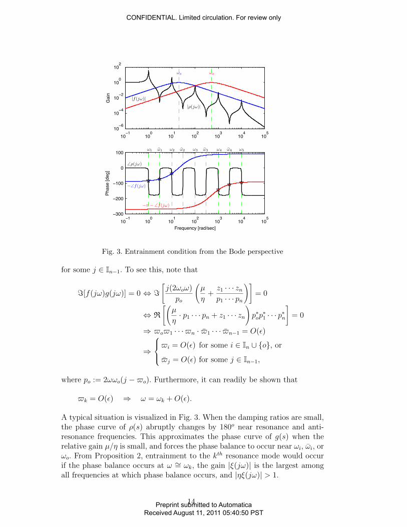
Fig. 3. Entrainment condition from the Bode perspective

for some j ∈ In−1. To see this, note that

=[f(jω)g(jω)] = 0 ⇔ =[j(2ωoω)

po

(µ

η+z1 · · · znp1 · · · pn

)]= 0

⇔ R

[(µ

η· p1 · · · pn + z1 · · · zn

)p∗op∗1 · · · p∗n

]= 0

⇒ $o$1 · · ·$n · $1 · · · $n−1 = O(ε)

⇒

$i = O(ε) for some i ∈ In ∪ {o}, or

$j = O(ε) for some j ∈ In−1,

where po := 2ωωo(j −$o). Furthermore, it can readily be shown that

$k = O(ε) ⇒ ω = ωk +O(ε).

A typical situation is visualized in Fig. 3. When the damping ratios are small,the phase curve of ρ(s) abruptly changes by 180o near resonance and anti-resonance frequencies. This approximates the phase curve of g(s) when therelative gain µ/η is small, and forces the phase balance to occur near ωi, ωi, orωo. From Proposition 2, entrainment to the kth resonance mode would occurif the phase balance occurs at ω ∼= ωk, the gain |ξ(jω)| is the largest amongall frequencies at which phase balance occurs, and |ηξ(jω)| > 1.

14



Consider the negative feedback case

η < 0, ωk−1 < ωo < ωk. (15)

The phase balance for this case occurs near resonance and anti-resonancemodes higher than ωo (see red curves in Fig. 3). Among these candidates foroscillations, the one with the largest gain |ξ(jω)| is expected to be stable.Since the gain at ωi is almost zero for small ε, oscillations near anti-resonancefrequencies would be unstable. The gain |f(jωi)| is smaller for higher frequencyωi. Hence, if the peak gain |g(jωi)| has the same decreasing property, so doesthe overall gain |ξ(jωi)|. Thus, the stable oscillation would occur at the lowestresonance mode ωk among those higher than ωo. Approximate entrainment tothe kth resonance mode would thus be expected if (15) holds, provided ζi, ζi,and |µ/η| are sufficiently small. This explains Proposition 3.

Next consider the positive feedback case

η > 0, ωk < ωo < ωk.

In this case, the phase balance occurs near resonance and anti-resonance modeslower than ωo (see blue curves in Fig. 3). Again, the predicted oscillationnear an anti-resonance is expected unstable because the gain |ξ(jωi)| is small.At resonance frequencies, the gain |f(jωi)| increases with i, while |g(jωi)|decreases with i. Hence, the two effects tend to cancel each other and thestability property depends on the magnitudes of the relative effects. Therefore,the mode to which stable entrainment occurs can be different for different planttransfer function g(s). It turns out that the CPG tends to entrain to the firstmode of resonance for the tensegrity structure studied later. In the other caseswhere

η > 0, ωk < ωo < ωk+1 or η < 0, ωk < ωo < ωk,

the phase balance occurs near ωo. Whether the oscillation at ω ∼= ωo is stableor unstable depends on the actual amount of damping and the location of ωowithin the interval between a resonance and an anti-resonance. Entrainmentto a resonance mode is not expected in these cases anyway.

3.4 Design by Mode Partition Diagrams

In the previous analysis, we have shown that the closed-loop system (4) isexpected to oscillate when |η| is sufficiently large, and that the frequency ω ofthe closed-loop oscillation is close to either a resonance frequency of the plantor the intrinsic frequency of the RIO, provided the plant has sufficiently smalldamping. For each controller parameter pair χ := (ωo, η/µ), the estimated

15



frequency ω(χ) is determined as the optimizer of (13). The basic questionsare: in which region of the controller parameter space χ, is ω(χ) close to aprescribed resonance frequency, and how to quantify the closeness when thedamping is nonzero? This section addresses these questions and develop acontrol design procedure.

The mode partition diagrams (MPDs) illustrate the expected entrainmentcharacteristics of the closed-loop system by separating the χ parameter spaceinto regions where entrained frequency ω(χ) is expected close to the kth res-onance frequency, the intrinsic RIO frequency, or neither. Let these sets bedenoted by Ok, Oo, and N, respectively. In particular, we define

Ok := {χ ∈ R2 : ek < εk, ek < ei, ∀ i ∈ In ∪ {o}\{k} }

Oo := {χ ∈ R2 : eo < εi, eo < ei, ∀ i ∈ In },(16)

where εi for i ∈ In are small numbers representing the error tolerance, and

ei(χ) :=

∣∣∣∣∣ω(χ)− ωiωi

∣∣∣∣∣ ,for i ∈ In ∪ {o}. The set N is defined by χ for which there is no feasiblesolution to (13) or the estimated closed-loop frequency ω(χ) is outside of theerror bound εi for all i. The MPD is obtained by visualizing the regions Ok,Oo, and N through numerical solutions to the optimization problem in (13)for selected grid points on the χ-plane . Once the MPD is found, the controllerparameter χ can be chosen from the region Ok of the desired resonance modek. A remaining question is how to set the error bounds εi for i ∈ In.

We will develop analytical bounds on the entrainment error in the frequencythrough a slight modification of a result in [9], which suggests the following:

εi :=

∣∣∣∣∣ ζi$oi

∣∣∣∣∣ , $oi :=

1

2

(ωoωi− ωiωo

).

To this end, note that the transfer function ρ(s) has a frequency responseillustrated in Fig. 3, and can be approximated by a second order transferfunction near a resonance mode. Let ρ(s) be an approximation of ρ(s) in theneighborhood of the kth resonance mode s ∼= jωk:

ρ(s) ∼= ρ(s) :=δkω

2k

s2 + 2ζkωks+ ω2k

where δk ∈ R is an appropriately chosen parameter. The following result canbe proved through a slight modification of results in [9, 10].

16



Proposition 4 Suppose the harmonic balance condition

1 = ηκ(a)f(jω)(µ/η + ρ(jω))

holds and the associated quasi-linear system is marginally stable. Then we have∣∣∣∣ω − ωkωk

∣∣∣∣ ≤∣∣∣∣∣ ζk$o

k

∣∣∣∣∣ if (ωo − ωk)(η/µ− 2$okζk/δk) > 0,

∣∣∣∣ω − ωoωo

∣∣∣∣ ≤∣∣∣∣∣ ζk$o

k

∣∣∣∣∣ if (ωo − ωk)η < 0.

Proof. The result is obtained by replacing η in [9] by (δk/2)η. 2

The error bound |ζk/$ok| is independent of the value of δk, and is determined

by the damping ζk and the distance $ok between ωk and ωo. Hence, the bound

is valid even if the approximation parameter value δk is inaccurate as longas the effects of the other poles and zeros in ρ(s) can be captured by a realconstant δk. In reality, the imaginary part of δk is close to but may not beexactly equal to zero, and this could potentially make the bound violated.However, we find the quantitative bounds useful in constructing MPDs.

We now summarize the procedure to solve the Resonance Entrainment Prob-lem to achieve closed-loop oscillations near a prescribed resonance mode k.

Design Procedure:

1. Find the scaling matrices Go and Ho as described in Section 3.1, and defineρ(s) as in (6).

2. Construct the MPD to identify the set Ok in (16) by solving the optimizationproblem (13), and choose a parameter pair (ωo, ηµ) ∈ Ok.

3. Choose a value for neuronal coupling strength µ > 0.4. Select actuation gain g to attain a desired amplitude of oscillation for the

plant output y at resonance, where the amplitude is estimated from y(t) ∼=<[yejωt] with y = P (jω)gGoκ(a)ea and a is given by (12) with ω = ωk.

5. Set the feedback gains G := gGo and H := hHo, where the sensory gain isdefined by h := η/g and η := µηµ.

6. The controller is given by Fig. 2 with the RIO given by (3), where theparameters G, H, ωo, µ are as specified above.

The controller thus designed is expected, by harmonic balance, to entrain tothe kth resonance mode with the frequency of the closed-loop oscillation ωsatisfying the error bound |(ω − ωk)/ωk| ≤ |ζk/$o

k|. The main design freedomis in Steps 2 and 3. In regards to Step 2, note that the further ωo is from thetargeted frequency ωk, the smaller the error bound |ζk/$o

k| becomes. Hence,the designer will want to maximize the distance |ωo − ωk|, while remaining inthe Ok region of the MPD. In Step 3, a choice µ > 1 will ensure that the RIO

17



oscillates autonomously without input (by Lemma 1 of [9]), but this is notnecessary for resonance entrainment.

4 Tensegrity Application

The design method outlined in the previous section is applied to the threecell tensegrity beam presented below. Accuracy of the MPD and robustnessof resonance entrainment are demonstrated by evaluating the design againstsimulations of a fully nonlinear model of the tensegrity dynamics.

4.1 Three cell beam

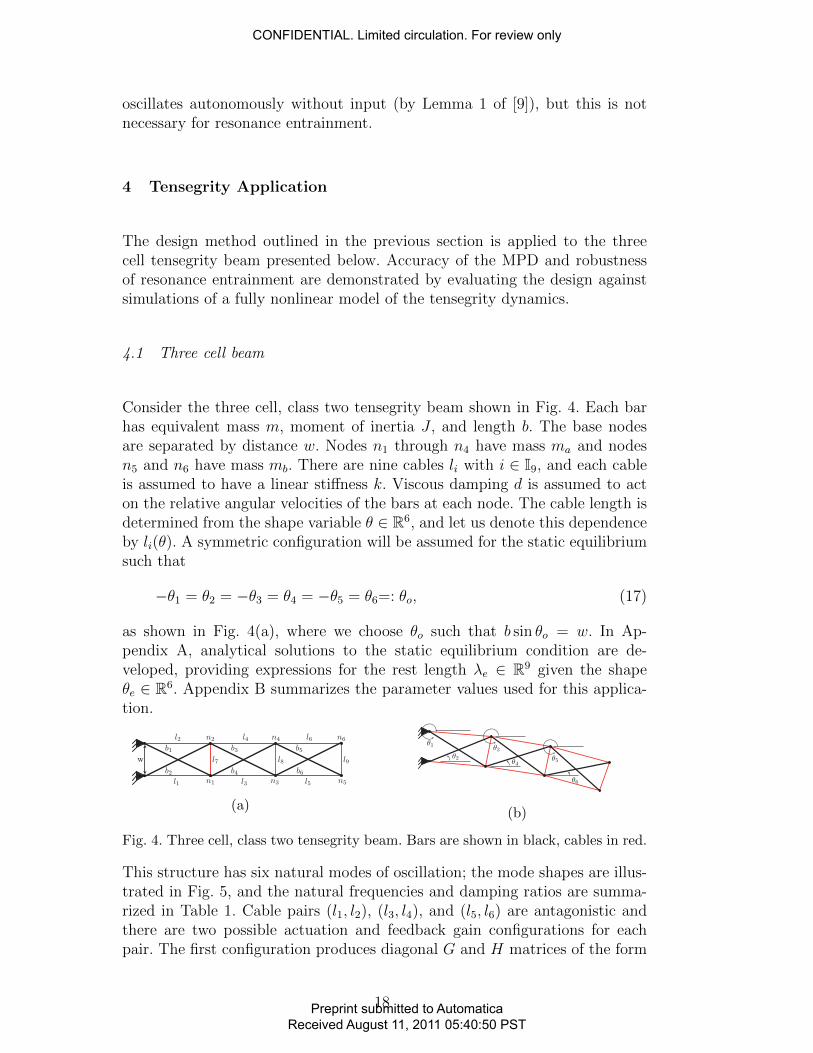
Consider the three cell, class two tensegrity beam shown in Fig. 4. Each barhas equivalent mass m, moment of inertia J , and length b. The base nodesare separated by distance w. Nodes n1 through n4 have mass ma and nodesn5 and n6 have mass mb. There are nine cables li with i ∈ I9, and each cableis assumed to have a linear stiffness k. Viscous damping d is assumed to acton the relative angular velocities of the bars at each node. The cable length isdetermined from the shape variable θ ∈ R6, and let us denote this dependenceby li(θ). A symmetric configuration will be assumed for the static equilibriumsuch that

−θ1 = θ2 = −θ3 = θ4 = −θ5 = θ6=: θo, (17)

as shown in Fig. 4(a), where we choose θo such that b sin θo = w. In Ap-pendix A, analytical solutions to the static equilibrium condition are de-veloped, providing expressions for the rest length λe ∈ R9 given the shapeθe ∈ R6. Appendix B summarizes the parameter values used for this applica-tion.

w

(a)(b)

Fig. 4. Three cell, class two tensegrity beam. Bars are shown in black, cables in red.

This structure has six natural modes of oscillation; the mode shapes are illus-trated in Fig. 5, and the natural frequencies and damping ratios are summa-rized in Table 1. Cable pairs (l1, l2), (l3, l4), and (l5, l6) are antagonistic andthere are two possible actuation and feedback gain configurations for eachpair. The first configuration produces diagonal G and H matrices of the form

18



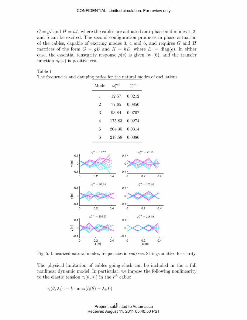
G = gI and H = hI, where the cables are actuated anti-phase and modes 1, 2,and 5 can be excited. The second configuration produces in-phase actuationof the cables, capable of exciting modes 3, 4 and 6, and requires G and Hmatrices of the form G = gE and H = hE, where E := diag(e). In eithercase, the essential tensegrity response ρ(s) is given by (6), and the transferfunction sρ(s) is positive real.

Table 1The frequencies and damping ratios for the natural modes of oscillations

Mode ωnati ζnati

1 12.57 0.0212

2 77.65 0.0850

3 93.84 0.0702

4 175.83 0.0274

5 204.35 0.0314

6 218.58 0.0086

0 0.2 0.4−0.1

0

0.1

y [m

]

0 0.2 0.4−0.1

0

0.1

0 0.2 0.4−0.1

0

0.1

y [m

]

0 0.2 0.4−0.1

0

0.1

0 0.2 0.4−0.1

0

0.1

y [m

]

x [m]0 0.2 0.4

−0.1

0

0.1

x [m]

Fig. 5. Linearized natural modes, frequencies in rad/sec. Strings omitted for clarity.

The physical limitation of cables going slack can be included in the a fullnonlinear dynamic model. In particular, we impose the following nonlinearityto the elastic tension τi(θ, λi) in the ith cable:

τi(θ, λi) := k ·max(li(θ)− λi, 0)

19



where max(x, 0) is equal to x when x ≥ 0 and is zero when x < 0. Theslack condition is ignored for the linearized model used in the control design,but is included in numerical simulations of the nonlinear dynamics for designevaluation.

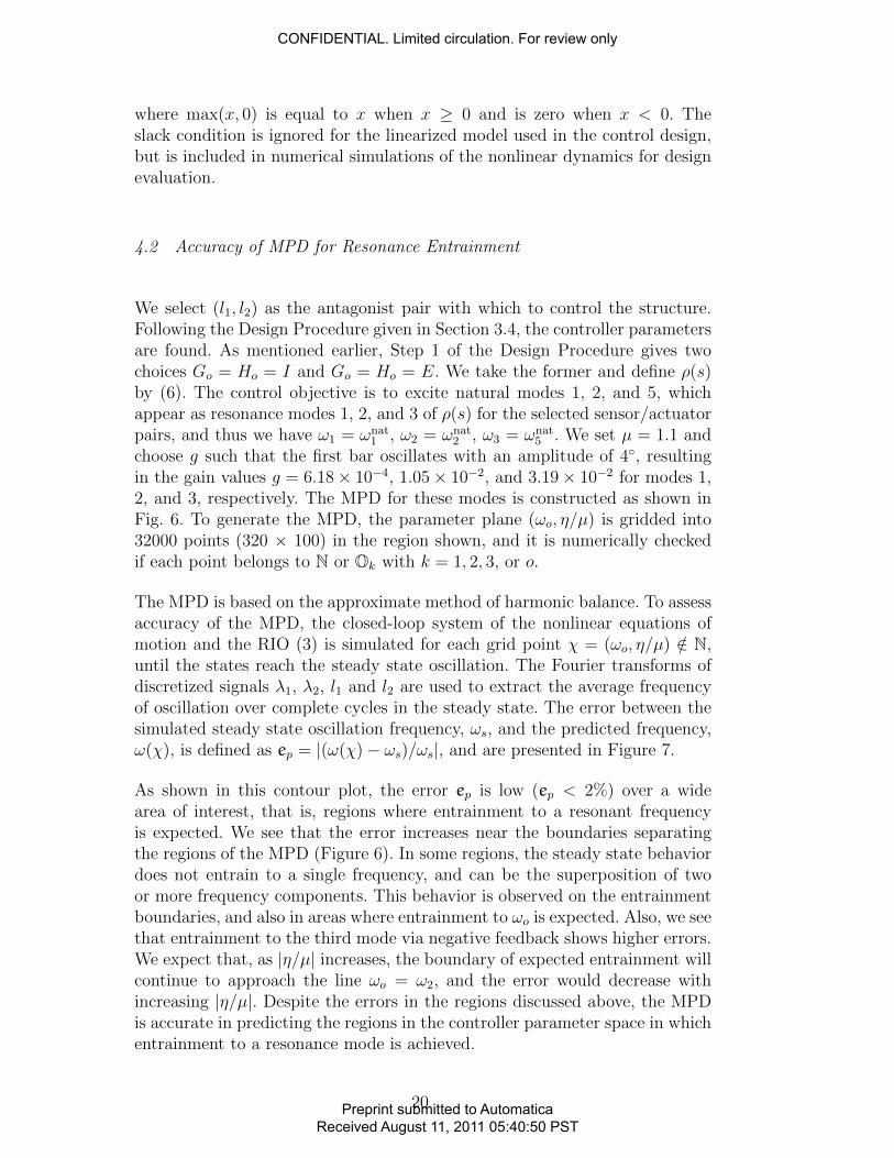
4.2 Accuracy of MPD for Resonance Entrainment

We select (l1, l2) as the antagonist pair with which to control the structure.Following the Design Procedure given in Section 3.4, the controller parametersare found. As mentioned earlier, Step 1 of the Design Procedure gives twochoices Go = Ho = I and Go = Ho = E. We take the former and define ρ(s)by (6). The control objective is to excite natural modes 1, 2, and 5, whichappear as resonance modes 1, 2, and 3 of ρ(s) for the selected sensor/actuatorpairs, and thus we have ω1 = ωnat

1 , ω2 = ωnat2 , ω3 = ωnat

5 . We set µ = 1.1 andchoose g such that the first bar oscillates with an amplitude of 4◦, resultingin the gain values g = 6.18× 10−4, 1.05× 10−2, and 3.19× 10−2 for modes 1,2, and 3, respectively. The MPD for these modes is constructed as shown inFig. 6. To generate the MPD, the parameter plane (ωo, η/µ) is gridded into32000 points (320 × 100) in the region shown, and it is numerically checkedif each point belongs to N or Ok with k = 1, 2, 3, or o.

The MPD is based on the approximate method of harmonic balance. To assessaccuracy of the MPD, the closed-loop system of the nonlinear equations ofmotion and the RIO (3) is simulated for each grid point χ = (ωo, η/µ) /∈ N,until the states reach the steady state oscillation. The Fourier transforms ofdiscretized signals λ1, λ2, l1 and l2 are used to extract the average frequencyof oscillation over complete cycles in the steady state. The error between thesimulated steady state oscillation frequency, ωs, and the predicted frequency,ω(χ), is defined as ep = |(ω(χ)− ωs)/ωs|, and are presented in Figure 7.

As shown in this contour plot, the error ep is low (ep < 2%) over a widearea of interest, that is, regions where entrainment to a resonant frequencyis expected. We see that the error increases near the boundaries separatingthe regions of the MPD (Figure 6). In some regions, the steady state behaviordoes not entrain to a single frequency, and can be the superposition of twoor more frequency components. This behavior is observed on the entrainmentboundaries, and also in areas where entrainment to ωo is expected. Also, we seethat entrainment to the third mode via negative feedback shows higher errors.We expect that, as |η/µ| increases, the boundary of expected entrainment willcontinue to approach the line ωo = ω2, and the error would decrease withincreasing |η/µ|. Despite the errors in the regions discussed above, the MPDis accurate in predicting the regions in the controller parameter space in whichentrainment to a resonance mode is achieved.

20



1 10 100−2

−1.5

−1

−0.5

0

0.5

1

1.5

2

Fig. 6. Mode partition diagram forthe three cell tensegrity beam, wherethe actuators are located at cables{l1, l2} and are used antagonistically;λ1 − λe1 = −(λ2 − λe2).

1 10 100−2

−1.5

−1

−0.5

0

0.5

1

1.5

2

0

2

4

6

8

10+%

Fig. 7. Percentage error between pre-dicted and entrained frequency. Theareas in white are contained in N ordid not give a steady state periodicoscillation.

4.3 Robustness of entrainment

As shown above, the harmonic balance condition is accurate in predictingthe closed-loop response. We have observed, however, that the error betweenthe predicted and simulated closed-loop frequencies increases as the linearizedtensegrity approximation begins to diverge from the nonlinear tensegrity be-havior. As an example, let us choose to target the first mode (k = 1) with thefirst bar oscillating at an amplitude of 30◦, giving g = 2.32 × 10−3 from ourdesign procedure. Numerical simulation results in the steady state oscillationshown in Fig. 8, where ωs = 11.74 rad/sec. This is outside of the predictederror bound (|ζ1/$o

1| = 2.0%, e1 = 6.6%), but we do note that the structure isroughly achieving its predicted oscillation amplitude. We also note that duringthe oscillation cycle, cables 1 and 2 are going slack, which causes a drop instiffness, and perhaps a drop in the resonance frequency.

For this reason, we study the nonlinear frequency response, presented in Fig. 9.For a given actuation amplitude g, the structure is driven by anti-phase sinu-soidal signals: λ1(t) = λa+g sin(ωt), λ2(t) = λa−g sin(ωt). For each frequencyω, the Hilbert transforms of discretized signals λ1, λ2, l1 and l2 are used toextract the average amplitude and phase over complete cycles, and comparedto the linearized system, ρ(s). As shown in Fig. 9, as the actuation amplitudeis increased, the resonant frequency decreases. This result is a combination oftwo factors, the first being the break down of the small angle approximationsused in the linearized model. Much like a pendulum’s increased period withincreasing amplitude, the same phenomenon is observed with the tensegritydynamics. The second factor is the slackening of cables near the nonlinear res-

21



89.5 90 90.5 91−30

−20

−10

0

10

20

30

Time [s]

[d

eg]

(a)

0 0.2 0.4

−0.2

0

0.2

x [m]

y [m

]

(b)

89.5 90 90.5 91−0.02

0

0.02

0.04

0.06

Time [s]

[m

]

(c)

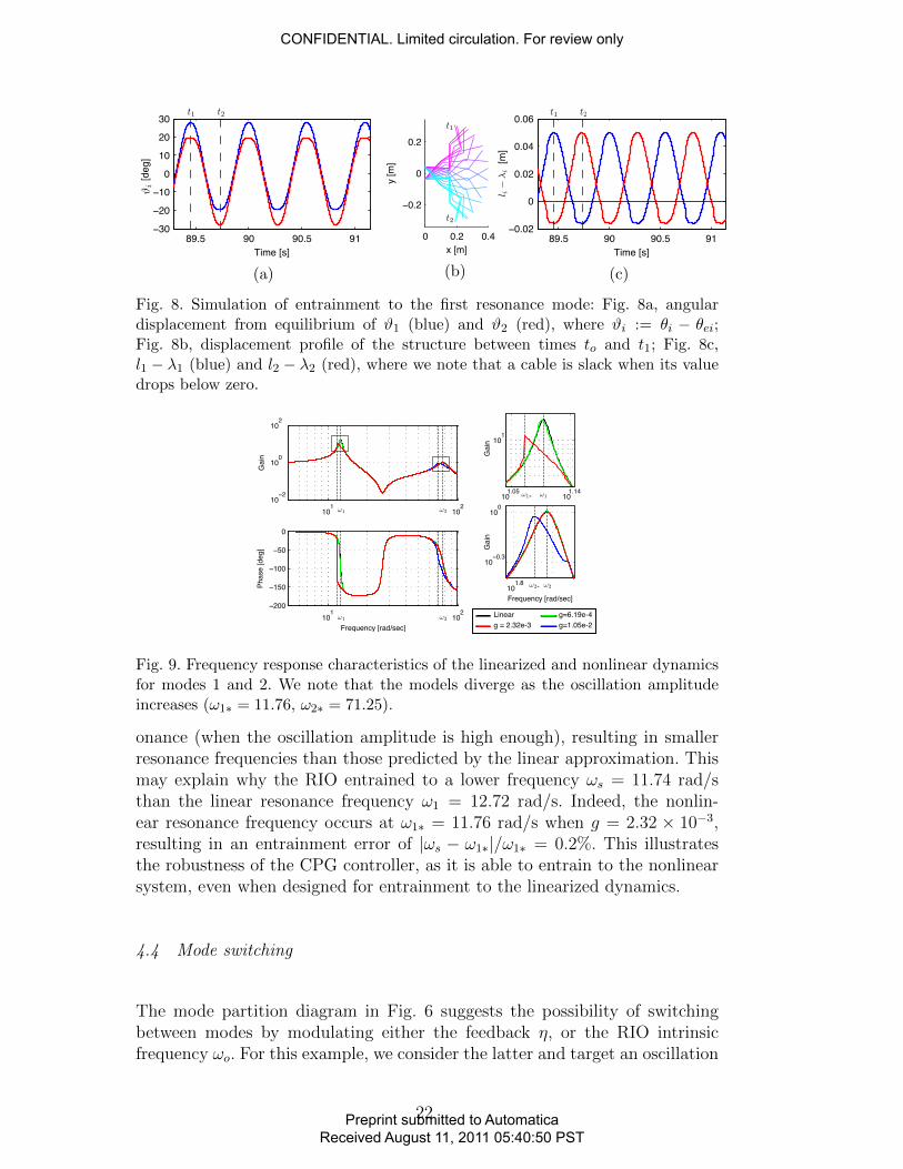
Fig. 8. Simulation of entrainment to the first resonance mode: Fig. 8a, angulardisplacement from equilibrium of ϑ1 (blue) and ϑ2 (red), where ϑi := θi − θei;Fig. 8b, displacement profile of the structure between times to and t1; Fig. 8c,l1 − λ1 (blue) and l2 − λ2 (red), where we note that a cable is slack when its valuedrops below zero.

101

102

10−2

100

102

Gai

n

101

102

−200

−150

−100

−50

0

Phas

e [d

eg]

Frequency [rad/sec]

Gai

n

Frequency [rad/sec]

101.05

101.14

101

101.8

10−0.3

100

Gai

n

Linearg = 2.32e-3

g=6.19e-4g=1.05e-2

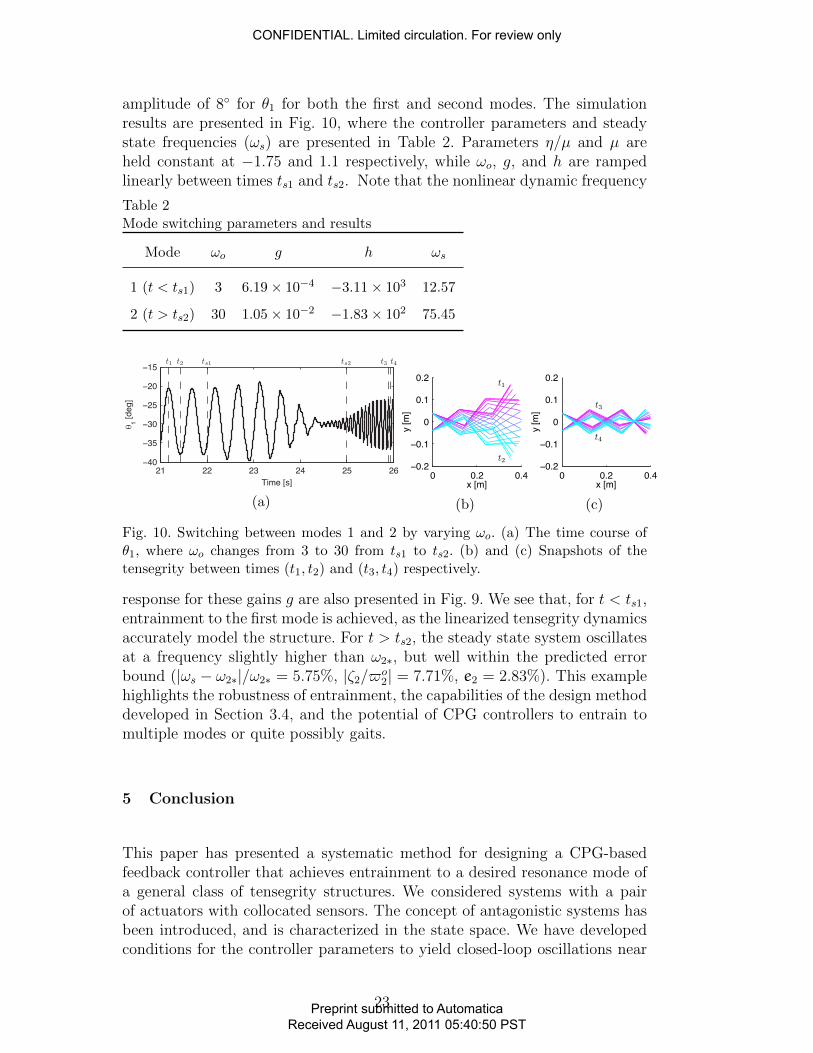
Fig. 9. Frequency response characteristics of the linearized and nonlinear dynamicsfor modes 1 and 2. We note that the models diverge as the oscillation amplitudeincreases (ω1∗ = 11.76, ω2∗ = 71.25).

onance (when the oscillation amplitude is high enough), resulting in smallerresonance frequencies than those predicted by the linear approximation. Thismay explain why the RIO entrained to a lower frequency ωs = 11.74 rad/sthan the linear resonance frequency ω1 = 12.72 rad/s. Indeed, the nonlin-ear resonance frequency occurs at ω1∗ = 11.76 rad/s when g = 2.32 × 10−3,resulting in an entrainment error of |ωs − ω1∗|/ω1∗ = 0.2%. This illustratesthe robustness of the CPG controller, as it is able to entrain to the nonlinearsystem, even when designed for entrainment to the linearized dynamics.

4.4 Mode switching

The mode partition diagram in Fig. 6 suggests the possibility of switchingbetween modes by modulating either the feedback η, or the RIO intrinsicfrequency ωo. For this example, we consider the latter and target an oscillation

22



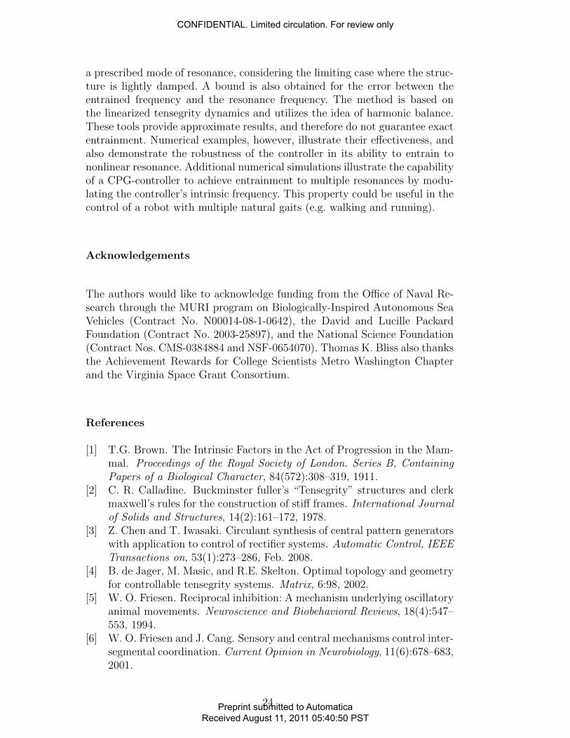
amplitude of 8◦ for θ1 for both the first and second modes. The simulationresults are presented in Fig. 10, where the controller parameters and steadystate frequencies (ωs) are presented in Table 2. Parameters η/µ and µ areheld constant at −1.75 and 1.1 respectively, while ωo, g, and h are rampedlinearly between times ts1 and ts2. Note that the nonlinear dynamic frequency

Table 2Mode switching parameters and results

Mode ωo g h ωs

1 (t < ts1) 3 6.19× 10−4 −3.11× 103 12.57

2 (t > ts2) 30 1.05× 10−2 −1.83× 102 75.45

21 22 23 24 25 26−40

−35

−30

−25

−20

−15

Time [s]

θ 1 [deg

]

(a)

0 0.2 0.4−0.2

−0.1

0

0.1

0.2

x [m]

y [m

]

(b)

0 0.2 0.4−0.2

−0.1

0

0.1

0.2

x [m]

y [m

]

(c)

Fig. 10. Switching between modes 1 and 2 by varying ωo. (a) The time course ofθ1, where ωo changes from 3 to 30 from ts1 to ts2. (b) and (c) Snapshots of thetensegrity between times (t1, t2) and (t3, t4) respectively.

response for these gains g are also presented in Fig. 9. We see that, for t < ts1,entrainment to the first mode is achieved, as the linearized tensegrity dynamicsaccurately model the structure. For t > ts2, the steady state system oscillatesat a frequency slightly higher than ω2∗, but well within the predicted errorbound (|ωs − ω2∗|/ω2∗ = 5.75%, |ζ2/$o

2| = 7.71%, e2 = 2.83%). This examplehighlights the robustness of entrainment, the capabilities of the design methoddeveloped in Section 3.4, and the potential of CPG controllers to entrain tomultiple modes or quite possibly gaits.

5 Conclusion

This paper has presented a systematic method for designing a CPG-basedfeedback controller that achieves entrainment to a desired resonance mode ofa general class of tensegrity structures. We considered systems with a pairof actuators with collocated sensors. The concept of antagonistic systems hasbeen introduced, and is characterized in the state space. We have developedconditions for the controller parameters to yield closed-loop oscillations near

23



a prescribed mode of resonance, considering the limiting case where the struc-ture is lightly damped. A bound is also obtained for the error between theentrained frequency and the resonance frequency. The method is based onthe linearized tensegrity dynamics and utilizes the idea of harmonic balance.These tools provide approximate results, and therefore do not guarantee exactentrainment. Numerical examples, however, illustrate their effectiveness, andalso demonstrate the robustness of the controller in its ability to entrain tononlinear resonance. Additional numerical simulations illustrate the capabilityof a CPG-controller to achieve entrainment to multiple resonances by modu-lating the controller’s intrinsic frequency. This property could be useful in thecontrol of a robot with multiple natural gaits (e.g. walking and running).

Acknowledgements

The authors would like to acknowledge funding from the Office of Naval Re-search through the MURI program on Biologically-Inspired Autonomous SeaVehicles (Contract No. N00014-08-1-0642), the David and Lucille PackardFoundation (Contract No. 2003-25897), and the National Science Foundation(Contract Nos. CMS-0384884 and NSF-0654070). Thomas K. Bliss also thanksthe Achievement Rewards for College Scientists Metro Washington Chapterand the Virginia Space Grant Consortium.

References

[1] T.G. Brown. The Intrinsic Factors in the Act of Progression in the Mam-mal. Proceedings of the Royal Society of London. Series B, ContainingPapers of a Biological Character, 84(572):308–319, 1911.

[2] C. R. Calladine. Buckminster fuller’s “Tensegrity” structures and clerkmaxwell’s rules for the construction of stiff frames. International Journalof Solids and Structures, 14(2):161–172, 1978.

[3] Z. Chen and T. Iwasaki. Circulant synthesis of central pattern generatorswith application to control of rectifier systems. Automatic Control, IEEETransactions on, 53(1):273–286, Feb. 2008.

[4] B. de Jager, M. Masic, and R.E. Skelton. Optimal topology and geometryfor controllable tensegrity systems. Matrix, 6:98, 2002.

[5] W. O. Friesen. Reciprocal inhibition: A mechanism underlying oscillatoryanimal movements. Neuroscience and Biobehavioral Reviews, 18(4):547–553, 1994.

[6] W. O. Friesen and J. Cang. Sensory and central mechanisms control inter-segmental coordination. Current Opinion in Neurobiology, 11(6):678–683,2001.

24



[7] R. B. Fuller. Tensile-integrity structures, U.S. Pat. 3063521, 1962.[8] H. Furuya. Concept of deployable tensegrity structures in space applica-

tion. International Journal of Space Structures, 7:143–151, 1992.[9] Y. Futakata and T. Iwasaki. Formal analysis of resonance entrainment by

central pattern generator. Journal of Mathematical Biology, 57(2):183–207, 2008.

[10] Y. Futakata and T. Iwasaki. Entrainment to natural oscillations viauncoupled central pattern generators. Automatic Control, IEEE Trans-actions on, 56(5):1075 –1089, May 2011.

[11] T. Glad and L. Ljung. Control Theory: Multivariable and Nonlinear Meth-ods. Taylor & Francis, New York, 2000.

[12] N.G. Hatsopoulos. Coupling the Neural and Physical Dynamics in Rhyth-mic Movements. Neural Computation, 8(3):567–581, 1996.

[13] T. Iwasaki. Multivariable harmonic balance for central pattern genera-tors. Automatica, 44(12):3061–3069, 2008.

[14] T. Iwasaki, S. Hara, and H. Yamauchi. Dynamical system design froma control perspective: Finite frequency positive-realness approach. IEEETransactions on Automatic Control, 48(8):1337, 2003.

[15] T. Iwasaki and M. Zheng. Sensory feedback mechanism underlying en-trainment of central pattern generator to mechanical resonance. BiologicalCybernetics, 94(4):245–261, 2006.

[16] N. Kanchanasaratool and D. Williamson. Motion control of a tensegrityplatform. Communications in Information and Systems, 2(3):299–324,2002.

[17] H. K. Khalil. Nonlinear Systems. Prentice Hall, New Jersey, 2002.[18] H. Kimura, S. Akiyama, and K. Sakurama. Realization of Dynamic Walk-

ing and Running of the Quadruped Using Neural Oscillator. AutonomousRobots, 7(3):247–258, 1999.

[19] W. B. Kristan Jr., R. L. Calabrese, and W. O. Friesen. Neuronal controlof leech behavior. Progress in Neurobiology, 76(5):279–327, 2005/8.

[20] M.A. Lewis and G.A. Bekey. Gait Adaptation in a Quadruped Robot.Autonomous Robots, 12(3):301–312, 2002.

[21] M.A. Lewis, R. Etienne-Cummings, M.J. Hartmann, Z.R. Xu, and A.H.Cohen. An in silico central pattern generator: silicon oscillator, cou-pling, entrainment, and physical computation. Biological Cybernetics,88(2):137–151, 2003.

[22] F. Li and R. E. Skelton. Sensor/actuator selection for tensegrity struc-tures. In 45th IEEE Conf. on Decision and Control, San Diego CA,December 2006. IEEE.

[23] J.L. Lin, K.C. Chan, J.J. Sheen, and S.J. Chen. Interlacing propertiesfor Mass-Dashpot-Spring Systems with proportional damping. Journalof dynamic systems, measurement, and control, 126(2):426–430, 2004.

[24] M. Masic and R. E. Skelton. Selection of prestress for optimal dynam-ic/control performance of tensegrity structures. International Journal ofSolids and Structures, 43:2110–2125, 2005.

25



[25] K.W. Moored and H. Bart-Smith. The Analysis of Tensegrity Structuresfor the Design of a Morphing Wing. Journal of Applied Mechanics, 74:668,2007.

[26] H. Murakami. Static and dynamic analyses of tensegrity structures. part1. nonlinear equations of motion. International Journal of Solids andStructures, 38:3599 – 3613, 2001.

[27] J. Nakanishi, J. Morimoto, G. Endo, G. Cheng, S. Schaal, and M. Kawato.Learning from demonstration and adaptation of biped locomotion.Robotics and Autonomous Systems, 47(2-3):79–91, 2004.

[28] G.N. Orlovsky, TG Deliagina, and S. Grillner. Neuronal Control of Lo-comotion: From Mollusc to Man. Oxford University Press, 1999.

[29] R. A. Pearce and W. O. Friesen. Intersegmental coordination of leechswimming: comparison of in situ and isolated nerve cord activity withbody wall movement. Brain Research, 299(2):363–366, 1984.

[30] S. Pellegrino and C. R. Calladine. Matrix analysis of statically and kine-matically indeterminate frameworks. International Journal of Solids andStructures, 22(4):409–428, 1986.

[31] R. E. Skelton. Dynamics of tensegrity systems: Compact forms. In 45thIEEE Conf. on Decision and Control, San Diego CA, December 2006.IEEE.

[32] R. E. Skelton and M. C. de Oliveira. Tensegrity Systems. Springer, 1stedition, June 2009.

[33] R. E. Skelton, J. P. Pinaud, and D. L. Mingori. Dynamics of the shell classof tensegrity structures. Journal of the Franklin Institute, 338:255–320,2001.

[34] KD Snelson. Continuous tension, discontinuous compression structures.US Patent, 1965.

[35] C. Sultan, M. Corless, and R. E. Skelton. A tensegrity flight simulator.Journal of Guidance, Control, and Dynamics, 23(6):1055–1064, 2000.

[36] C. Sultan, M. Corless, and R. E. Skelton. Linear dynamics of tensegritystructures. Engineering Structures, 24(6):671–685, 2002.

[37] C. Sultan and R. Skelton. Deployment of tensegrity structures. Interna-tional Journal of Solids and Structures, 40(18):4637–4657, 2003.

[38] C. Sultan and R.E. Skelton. Tendon control deployment of tensegritystructures. In Proceedings of the SPIE 5th Symposium on Smart Struc-tures and Materials. SPIE, 1998.

[39] G. Taga, Y. Yamaguchi, and H. Shimizu. Self-organized control of bipedallocomotion by neural oscillators in unpredictable environment. BiologicalCybernetics, 65(3):147–159, 1991.

[40] BW Verdaasdonk, H. Koopman, and F.C.T.V.D. Helm. Energy efficientand robust rhythmic limb movement by central pattern generators. Neu-ral Networks, 19(4):388–400, 2006.

[41] B.W. Verdaasdonk, H.F.J.M. Koopman, and F.C.T. Van der Helm. Reso-nance tuning in a neuro-musculo-skeletal model of the forearm. BiologicalCybernetics, 96(2):165–180, 2007.

26



[42] C.A. Williams and S.P. DeWeerth. A comparison of resonance tuningwith positive versus negative sensory feedback. Biological Cybernetics,96(6):603–614, 2007.

[43] M. M. Williamson. Neural control of rhythmic arm movements. NeuralNetworks, 11:1379–1394, 1998.

[44] X. Yu, B. Nguyen, and W. O. Friesen. Sensory feedback can coordinatethe swimming activity of the leech. Journal of Neuroscience, 19(11):4634–4643, 1999.

A Symmetric Prestressable Configuration

Consider the tensegrity shown in Fig. 4a. We will derive a condition on therest length λe such that static equilibrium is achieved at the symmetric con-figuration (17) with b sin θo = w. All cables are assumed linearly elastic withuniform spring constant k. Solving the static equilibrium equations for λe withthese geometric constraints produces a solution where λe1 = λe2, λe3 = λe4,λe5 = λe6, with λe7, λe8 and λe9 as functions of λe1, λe3, and λe5. To reducethe number of free parameters, assume λe1 = . . . = λe6 =: λa. This allows λeto be expressed in terms of one free parameter, λa:

λe7 = λe8 =2wλala− w, λe9 =

wλala

,

where la :=√b2 − w2. The following condition enforces all cables to be in

tension,

0 < λa < la, 0 < {λe7, λe8, λe9} < w,

which reduces to

la2< λa < la.

This result leads to a stiffness matrix with two free parameters, the springconstant k of the cables and λa. This allows the designer to select appropriatematerials for a physical model, then adjust the pretension using λa to targetspecific dynamic properties like natural frequency.

B Tensegrity Beam Parameters

27



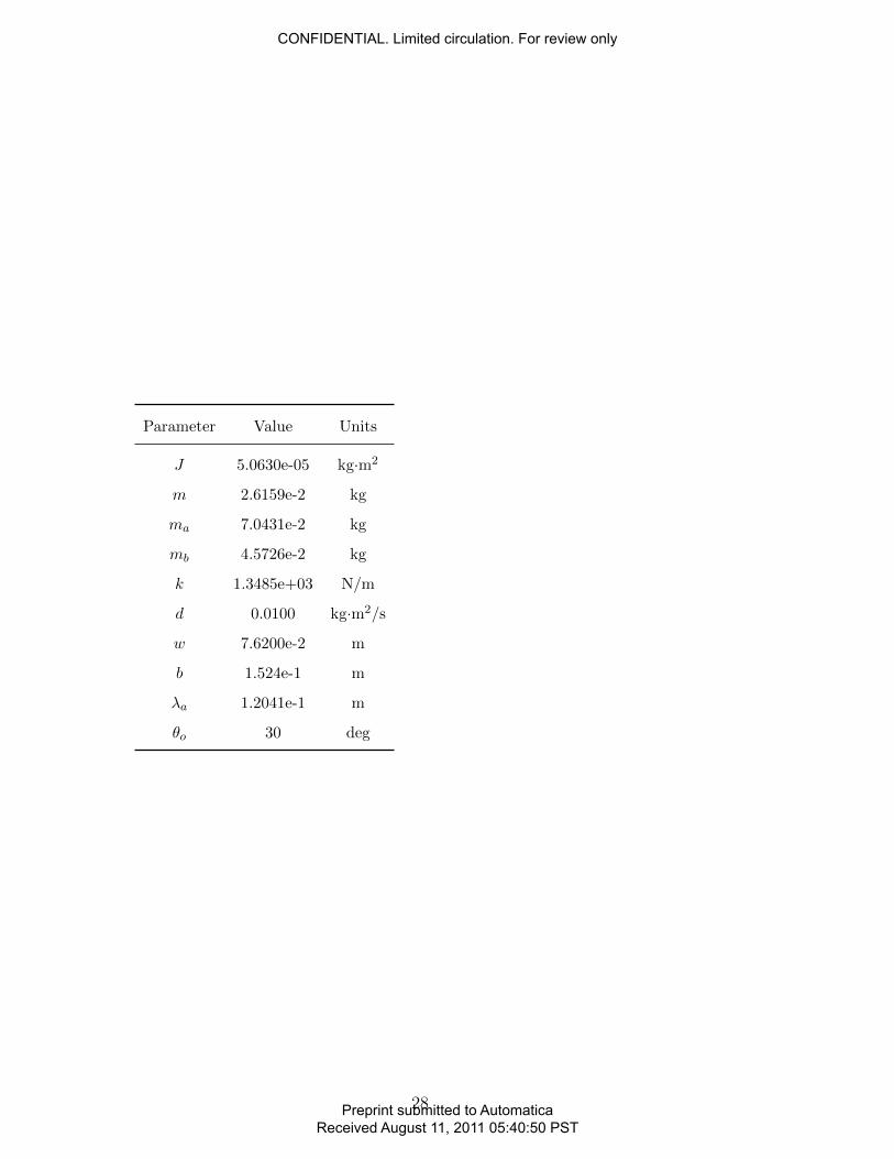
Parameter Value Units

J 5.0630e-05 kg·m2

m 2.6159e-2 kg

ma 7.0431e-2 kg

mb 4.5726e-2 kg

k 1.3485e+03 N/m

d 0.0100 kg·m2/s

w 7.6200e-2 m

b 1.524e-1 m

λa 1.2041e-1 m

θo 30 deg

28



Documents

Resonance Entrainment of Tensegrity Structures via CPG Control · Resonance Entrainment of Tensegrity Structures via CPG Control Thomas K. Bliss a, Tetsuya Iwasaki b, Hilary Bart-Smith