Revisiting the Turbulent Prandtl Number in an Idealized Atmospheric Surface Layer

DAN LI

Program in Atmospheric and Oceanic Sciences, Princeton University, Princeton, New Jersey

GABRIEL G. KATUL

Nicholas School of the Environment, and Department of Civil and Environmental Engineering,

Duke University, Durham, North Carolina

SERGEJ S. ZILITINKEVICH

Finnish Meteorological Institute, and Division of Atmospheric Sciences, University of Helsinki, Helsinki, Finland, and Department

of Radio Physics, N.I. Lobachevski State University of Nizhniy, Novgorod, and Faculty of Geography, Moscow University, and

Institute of Geography, Russian Academy of Sciences, Moscow, Russia, and Nansen Environmental and Remote Sensing

Center/Bjerknes Centre for Climate Research, Bergen, Norway

(Manuscript received 10 November 2014, in final form 8 March 2015)

ABSTRACT

Cospectral budgets are used to link the kinetic and potential energy distributions of turbulent eddies, as

measured by their spectra, to macroscopic relations between the turbulent Prandtl number (Prt) and atmo-

spheric stability measures such as the stability parameter z, the gradient Richardson number Rg, or the flux

Richardson number Rf in the atmospheric surface layer. The dependence of Prt on z, Rg, or Rf is shown to be

primarily controlled by the ratio of Kolmogorov and Kolmogorov–Obukhov–Corrsin phenomenological

constants and a constant associated with isotropization of turbulent flux production that can be independently

determined using rapid distortion theory in homogeneous turbulence. Changes in scaling laws of the vertical

velocity and air temperature spectra are also shown to affect the Prt–z (or Prt–Rg or Prt–Rf) relation. Results

suggest that departure of Prt from unity under neutral conditions is induced by dissimilarity between mo-

mentum and heat in terms of Rotta constants, isotropization constants, and constants in the flux transfer

terms. A maximum flux Richardson number Rfm predicted from the cospectral budgets method (50.25) is in

good agreement with values in the literature, suggesting that Rfm may be tied to the collapse of Kolmogorov

spectra instead of laminarization of turbulent flows under stable stratification. The linkages between mi-

croscale energy distributions of turbulent eddies andmacroscopic relations that are principally determined by

dimensional considerations or similarity theories suggest that when these scalewise energy distributions of

eddies experience a ‘‘transition’’ to other distributions (e.g., when Rf is increased over Rfm), dimensional

considerations or similarity theories may fail to predict bulk flow properties.

1. Introduction

The significance of exchanges of momentum, heat, wa-

ter vapor, and trace gases such as CO2 and CH4 between

the earth’s surface and the atmospheric boundary layer

(ABL) is rarely questioned (Brutsaert 1982; Stull 1988;

Baldocchi et al. 2001; Stensrud 2007). These exchanges are

governed by turbulence in the lower atmosphere, which is

generated by both shear and buoyancy forces (Obukhov

1946; Monin and Obukhov 1954). It is often assumed that

the turbulent transport of heat (as well as other scalars,

such as water vapor and CO2) is similar to the turbulent

transport of momentum, given that the same eddies are

the transporting agent for momentum, heat, and scalars.

This assumption is often referred to as the Reynolds

analogy (Kays 1994) and is used extensively in applications

where eddy diffusivities are required. However, dissimi-

larity between turbulent transport of momentum and

scalars for unstable stratification has been well docu-

mented in the ABL even prior to the weighty Kansas

experiments (Businger et al. 1971; Brutsaert 2005).

Corresponding author address:Dan Li, Program in Atmospheric

and Oceanic Sciences, Princeton University, 300 Forrestal Road,

Sayre Hall, Princeton, NJ 08544.

E-mail: danl@princeton.edu

2394 JOURNAL OF THE ATMOSPHER IC SC IENCES VOLUME 72

DOI: 10.1175/JAS-D-14-0335.1

� 2015 American Meteorological Society

The turbulent Prandtl number (Prt), a non-

dimensional number defined by the ratio of turbulent

diffusivities of momentum and heat (Kays 1994), is

commonly used to account for such dissimilarity. It is an

important parameter in closure schemes for the

Reynolds-averaged Navier–Stokes equations (Mellor

and Yamada 1974; Stull 1988) and a similar parameter

(i.e., the subgrid-scale Prandtl number) is also widely

used in large-eddy simulation (LES) (Lilly 1992; Bou-

Zeid et al. 2008). Numerous studies have reported Prt in

wall-bounded turbulent boundary layers under ‘‘ideal’’

laboratory conditions (Yakhot et al. 1987; Kays 1994)

and are not reviewed here. In the logarithmic region,

where the Prt is expected to be a constant for fluids with

molecular Prandtl number (Prm, the ratio of kinematic

viscosity and molecular thermal diffusivity) of order

unity such as air and water, the value of Prt reported in

the literature ranges from 0.73 to 0.92 (Kays 1994). The

Prt values reported in the well-studied atmospheric

surface layer (ASL), which is the lowest 50–100m of the

ABL and corresponds to the logarithmic region re-

ported in laboratory experiments (Businger et al. 1971;

Högström 1988), exhibit much larger scatter even for

near-neutral conditions (i.e., in the absence of buoyancy

flux at the surface). Moreover, Prt in the ASL is further

affected by the thermal stratification or atmospheric

stability (Businger et al. 1971; Högström 1988; Li and

Bou-Zeid 2011; Li et al. 2012). Explaining the causes of

variability in the turbulent Prandtl number frames the

scope of this work.

Despite significant advances in experiments and nu-

merical simulations, a unified phenomenological theory

that (i) elucidates possible departures of Prt from unity

under near-neutral conditions, (ii) predicts variations of

Prt with atmospheric stability from unstable through

stable stratification in the ASL, and (iii) captures the

impacts of various physical processes, such as flux

transport terms, on Prt is currently lacking. Few recent

studies (Katul et al. 2011; Li et al. 2012) have attempted

to unravel the impact of thermal stratification on Prt in

the ASL building on recent phenomenological argu-

ments developed for the mean velocity profile in pipes

(Gioia et al. 2010). In those studies, it was conjectured

that the quasi-universal behavior of Prt with atmo-

spheric stability parameters in the ASL may be con-

nected to the quasi-universal spectral shapes whose

finescales are reasonably described by Kolmogorov’s

theory in the inertial subrange (Katul et al. 2011; Li et al.

2012). Two recent studies formalized these linkages by

analytically solving cospectral budgets for momentum

and heat fluxes with prescribed idealized spectral shapes

for vertical velocity and air temperature anchored to

Kolmogorov’s phenomenological theory at small scales

(Katul et al. 2013b, 2014). The cospectral budgets method

was shown to reproduce many bulk relations reported in

experiments, simulations, and othermodels (Yamada 1975;

Zilitinkevich et al. 2008, 2013), including the variation of Prtwith atmospheric stability parameters. These studies sug-

gest that linkages must exist between the spectral shapes of

vertical velocity and air temperature and the bulk relations

for the mean flow, which are principally determined from

dimensional considerations or similarity theories.

Building on these phenomenological studies, the ob-

jective of this work is to generalize earlier phenome-

nological theories so that they can accommodate

measured alterations in scaling laws in vertical velocity

and air temperature spectra as atmospheric stability

changes (Kader and Yaglom 1991). The dependence of

Prt on other important physical processes that have not

been considered in previous studies is also analyzed

over a wide range of atmospheric stability conditions.

The work here aims to link the spectral shapes of vertical

velocity and air temperature, which describe the mi-

croscale states of turbulent kinetic and potential energy

distributions, as shall be seen later, to the bulk flow

properties, such as Prt. This linkage is particularly impor-

tant for improving atmospheric modeling, because turbu-

lence in the ABL spans an enormous range of scales, and

different physical processes occur at different scales, which

cannot be fully captured by parameterizations of bulk flow

properties that are widely used in current numerical

weather and climatemodels (Stensrud 2007). For example,

there is strong coupling between small-scale turbulence

and microphysical/aerosol processes (Bodenschatz et al.

2010). Moreover, the fast degeneration of small-scale

turbulence but the long lifetime of large-scale turbu-

lence after sunset is a key for maintaining turbulent

mixing during nighttime in the ABL (Stull 1988).

The paper is organized as follows. Section 2 presents

the theory, including the cospectral budgets for mo-

mentum and heat fluxes and how they are solved with

the aid of idealized spectral shapes for vertical velocity

and air temperature. Section 3 presents the resulting

solution and compares the solution to experiments and

other models, and section 4 concludes with the impli-

cations of these results to ASL flows.

2. Theory

a. Background and definitions

The turbulent Prandtl number is defined as (Kays

1994)

Prt 5Km

Kh

52u0w0/S2w0T 0/G

, (1)

JUNE 2015 L I E T AL . 2395

where Km and Kh are turbulent or eddy diffusivities for

momentum and heat, respectively; the overbar denotes

averaging over coordinates of statistical homogeneity;

u0, w0, and T 0 are turbulent fluctuations of the longitu-

dinal velocity, vertical velocity, and air temperature,

respectively, from their averages; u0w0 is the turbulent

momentum flux; w0T 0 is the turbulent sensible heat flux;S5 ›U(z)/›z is the mean velocity gradient; and

G5 ›T(z)/›z is the mean air temperature gradient. To

describe thermal stratification effects on S and G as well

as other flow statistics, Monin–Obukhov similarity the-

ory (MOST), is commonly employed (Obukhov 1946;

Monin and Obukhov 1954; Businger and Yaglom 1971).

MOST assumes that the flow in the ASL is stationary,

planar homogeneous, and without subsidence, charac-

terized by sufficiently high Reynolds and Peclet num-

bers so that viscous and molecular diffusion effects are

negligible compared to Km and Kh. When these as-

sumptions are applied to the mean momentum and

mean temperature budgets, the resulting outcome is that

u0w0 and w0T 0 become independent of height z. It is for

this reason that the idealized ASL is also labeled as the

constant-flux region. Using only dimensional consider-

ations, Monin and Obukhov showed that distortions to

the classical logarithmic velocity and air temperature

profiles by buoyancy can be accounted for by stability

correction functions fm and fh (Obukhov 1946; Monin

and Obukhov 1954; Businger and Yaglom 1971), re-

spectively, given as follows:

fm(z)5kz

u*S and (2)

fh(z)5kz

T*G , (3)

where k’ 0:4 is the von Kármán constant, z is height

from the ground surface or zero-plane displacement and

is assumed to be much larger than the depth of the vis-

cous sublayer, u*5 (2u0w0)1/2 is the friction velocity,

and T*52w0T 0/u* is a temperature scaling parameter.

The stability parameter is defined as z5 z/L, with

L52u3*/(kbw0T 0

y) being the Obukhov length (Obukhov

1946); b5 g/Ty is the buoyancy parameter; g is the grav-

itational acceleration; and Ty is the virtual temperature,

with T21y being the coefficient of expansion for an ideal

gas. For simplicity, the virtual temperature is approximated

by the air temperature here given the minor impact water

vapor flux has on the overall buoyancy flux. When z, 0,

the ASL is unstable (e.g., during daytime over land); and

when z. 0, the ASL is stable (e.g., during nighttime over

land).When z’ 0, theASL is labeled as neutrally buoyant

(or neutral), and no significant density gradients are ex-

pected due to surface heating or cooling.

Based on these definitions, Prt can be related to the

stability correction functions using

Prt 5fh(z)

fm(z). (4)

b. Cospectral budgets of momentum and heat fluxes

The turbulent momentum and heat fluxes are linked

to eddy sizes or wavenumbers using the cospectral

definitions:

u0w05ð‘0Fuw(K) dK and (5)

w0T 0 5ð‘0FwT(K) dK , (6)

where Fuw(K) is the cospectrum of u0 and w0; FwT(K) is

the cospectrum of w0 and T 0; andK is a one-dimensional

wavenumber in the streamwise direction. This definition

of K is selected here to be consistent with the myriad of

ASL experiments (Kaimal et al. 1972; Kaimal 1973;

Kaimal and Finnigan 1994; Wyngaard and Cote 1972)

that report spectra and cospectra from single-point time

series measurements converted to one-dimensional

streamwise wavenumber using Taylor’s frozen turbu-

lence hypothesis (Taylor 1938).

Before the cospectral budgets of momentum and

sensible heat fluxes are presented, a brief summary of

the main budgets of momentum and heat fluxes in the

idealized ASL is provided. These budgets are

›u0w0

›t5 052w0w0S2

›w0w0u0

›z2

1

ru0›p0

›z

1bu0T 0 2 2n›u0

›z

›w0

›zand (7)

›w0T 0

›t5 052w0w0G2

›w0w0T 0

›z2

1

rT 0›p

0

›z

1bT 0T 0 2 (n1Dm)›w0

›z

›T 0

›z, (8)

where r is the mean air density, p is the air pressure, n is

the kinematic viscosity, andDm is the molecular thermal

diffusivity. The molecular Prandtl number of air is de-

fined as Prm 5 n/Dm ’ 0:72. The terms on the left-hand

side of the equations represent changes in covariances

(i.e., u0w0 and w0T 0) with time. The terms on the right-

hand side of the equations represent (in order): pro-

duction terms due to the presence of mean velocity and

air temperature gradients (2w0w0S and 2w0w0G), fluxtransport terms that represent turbulent transport

of momentum and heat fluxes (2›w0w0u0/›z and

2396 JOURNAL OF THE ATMOSPHER IC SC IENCES VOLUME 72

2›w0w0T 0/›z), pressure decorrelation terms due

to interactions between pressure and velocity

[2(1/r)u0(›p0/›z)] and between pressure and tempera-

ture [2(1/r)T 0(›p0/›z)], buoyancy terms arising from

thermal stratification in the ASL (bu0T 0 and bT 0T 0), andmolecular destruction terms [22n(›u0/›z)(›w0/›z) and

2(n1Dm)(›w0/›z)(›T 0/›z)].In correspondence, the cospectral budgets of mo-

mentum and heat fluxes in the ASL can be simplified as

follows (Panchev 1971; Bos et al. 2004; Bos and

Bertoglio 2007; Canuto et al. 2008; Katul et al. 2013a):

›Fuw(K)

›t5 05Puw(K)1Tuw(K)1pu(K)

1bFuT(K)2 2nK2Fuw(K) and (9)

›FwT(K)

›t5 05PwT(K)1TwT(K)1pT(K)

1bFTT(K)2 (n1Dm)K2FwT(K) . (10)

The terms on the left-hand side of the equations represent

temporal changes in the cospectra. The terms on the right-

hand side of the equations represent (in order): production

P, flux transfer T, pressure decorrelation p, buoyancy

(bFuT andbFTT), andmolecular destruction. The termFuT

is the cospectrum of u0 andT 0, and FTT(K) is the spectrum

of air temperature. The molecular destruction terms are

assumed to be small since they are, in principle, significant

at sufficiently largewavenumber on the order of 1/h, where

h is the Kolmogorov microscale scale (on the order of 0.1–

1mm in the ASL). This is essentially assuming that eddies

with sizes on the order of h do not contribute significantly

to momentum and heat fluxes (at least when compared to

othermechanisms such asp). The term FuT(K) is assumed

to be small compared toPuw(K) and can be ignored. This is

because it involves the correlation between the turbulent

longitudinal velocity and air temperature, which is often

small in the ASL, as demonstrated using direct numerical

simulations (DNS) (Katul et al. 2014; Shah and Bou-Zeid

2014) and scaling arguments (Stull 1988). Hence, as a

starting point, the cospectral budgets of momentum and

heat fluxes here involve only themost basic terms common

to all models and are given by

Puw(K)1Tuw(K)1pu(K)5 0 and (11)

PwT(K)1TwT(K)1pT(K)1bFTT(K)5 0. (12)

The production terms can be obtained from direct

Fourier transforming 2w0w0S and 2w0w0G:

Puw(K)52Fww(K)S and (13)

PwT(K)52Fww(K)G , (14)

where Fww(K) is the vertical velocity spectrum.

The flux transfer terms act to transport fluxes away

from the peak of the cospectra; hence, they are param-

eterized using a spectral gradient diffusion model as

follows (Bos et al. 2004; Bos and Bertoglio 2007):

Tuw(K)52AUU

›

›K[«1/3K5/3Fuw(K)] and (15)

TwT(K)52ATT

›

›K[«1/3K5/3FwT(K)] , (16)

whereAUU andATT aremodel constants associated with

the flux transfer terms and « is the mean dissipation rate

of the turbulent kinetic energy (TKE). Throughout, the

term ‘‘flux transport’’ is used in the context of Reynolds-

averaged equation, while the term ‘‘flux transfer’’ is used

in spectral space. It is also conceivable that the flux

transport terms are negligible in an idealized ASL, but

the flux transfer terms can be significant at a given K.

To model the pressure decorrelation terms, a Rotta-

type parameterization is invoked in the spectral domain

and corresponds to the one widely used in second-order

closure schemes (Mellor and Yamada 1974; Yamada

1975). The limitations of such a Rotta approach are

reasonably established (Choi and Lumley 2001); how-

ever, this parameterization remains the primary ‘‘work

horse’’ model to close pressure-scalar and pressure-

velocity covariances with some success (Launder et al.

1975). The following standard closure formulations are

employed here (Launder et al. 1975; Pope 2000):

pu(K)52AU

Fuw(K)

tuw(K)2CIUPuw(K) and (17)

pT(K)52AT

FwT(K)

twT(K)2CITPwT(K) , (18)

where AT and AU (’1.8) are the Rotta constants (Pope

2000), CIT and CIU (’3/5) are constants associated with

isotropization of production terms (herein referred to as

the isotropization constants), which can be determined

using rapid distortion theory in homogeneous turbu-

lence (Pope 2000). The parameters tuw(K) and twT(K)

are relaxation time scales for momentum and heat

fluxes, respectively, which are also wavenumber de-

pendent. A widely used formulation for tuw(K) and

twT(K) is given by the following (Corrsin 1961; Bos et al.

2004; Bos and Bertoglio 2007; Cava and Katul 2012;

Katul et al. 2014):

tuw(K)5 twT(K)5 «21/3K22/3 . (19)

With these parameterizations, Eqs. (11) and (12) re-

duce to

JUNE 2015 L I E T AL . 2397

›Fuw(K)

›K1

�AU

AUU

15

3

�K21Fuw(K)

52(12CIU)S

AUU«1/3

Fww(K)K25/3 and (20)

›FwT(K)

›K1

�AT

ATT

15

3

�K21FwT(K)

52(12CIT)G

ATT�1/3

Fww(K)K25/3

1b

ATT«1/3

FTT(K)K25/3 . (21)

The above equations for Fuw(K) and FwT(K) can be

solved once Fww(K) and FTT(K) are known or specified.

The precise spectral shapes of Fww(K) and FTT(K) will

be discussed later. However, for illustration purposes, it

is convenient to begin with a single power-law formu-

lation with Fww(K)5CwwK2a and FTT(K)5CTTK

2g,

where a and g are spectral scaling exponents and Cww

and CTT are normalization factors.

c. Solving the cospectral budgets for momentum andheat fluxes

Equations (20) and (21) reduce to two (uncoupled) first-

order ordinary differential equations, given as follows:

dFuw(K)

dK1D1K

21Fuw(K)5D2CwwK2a25/3 and

(22)

dFwT(K)

dK1D3K

21FwT(K)5D4CwwK2a25/3

1D5CTTK2g25/3 , (23)

where D15AU /AUU 15/3, D252(12CIU)S/(AUU«1/3),

D3 5 AT /ATT 1 5/3, D4 5 2(12 CIT)G/(ATT«1/3), and

D55b/(ATT«1/3). These two equations can be solved to

yield the following:

Fuw(K)5D2

2a2 2/31D1

CwwK2a22/31E1K

2D1 and

(24)

FwT(K)5D4

2a2 2/31D3

CwwK2a22/3

1D5

2g2 2/31D3

CTTK2g22/31E2K

2D3 ,

(25)

where E1 and E2 are integration constants to be de-

termined later. The above solutions implicitly require

D1 $a1 2/3 and D3 $max(a1 2/3, g1 2/3). That is,

AU /AUU $a2 1, and AT /ATT $max(a2 1, g2 1).

d. Idealized spectral shapes of Fww(K) and FTT(K)

In this section,multiexponent approximations toFww(K)

and FTT(K) are evaluated so that Eqs. (24) and (25) can be

integrated across all K so as to obtain the momentum and

heat fluxes. One plausible approximation assumes that the

spectra of vertical velocity and temperature simply follow

the Kolmogorov 25/3 scaling for all K.Ka and level off

for all K,Ka for near-neutral and stable stratification,

where Ka ’ 1/z is a transition wavenumber delineating

attached eddies to the boundary from detached eddies as-

sumed to follow inertial subrange scaling (Katul et al.

2014). An outcome of this approximation is a connection

between AU , CIU , the Kolmogorov phenomenological

constant Co in the inertial subrange, and the von Kármánconstant k (Katul et al. 2014). Later, this idealized spectral

shape ofFTT(K) wasmodified inLi et al. (2015,manuscript

submitted to Bound.-Layer Meteor.) to accommodate the

presence of 21 scaling in the low-wavenumber part based

on ASL measurements above lakes and glaciers. Both

studies (Katul et al. 2014; Li et al. 2015, manuscript sub-

mitted to Bound.-Layer Meteor.) focused on stable ASL

conditions and did not consider any effects of flux transfer

terms in their analyses. Other studies did consider flux

transfer terms in their scalar cospectral budgets (Cava and

Katul 2012; Katul et al. 2013a), but these studies primarily

focused on the effects of flux transfer terms on inertial

subrange scales, not on bulk flow properties.

More realistic spectral shapes are assumed here for

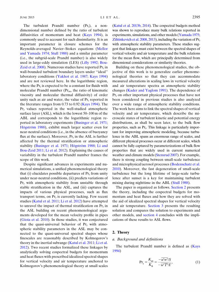
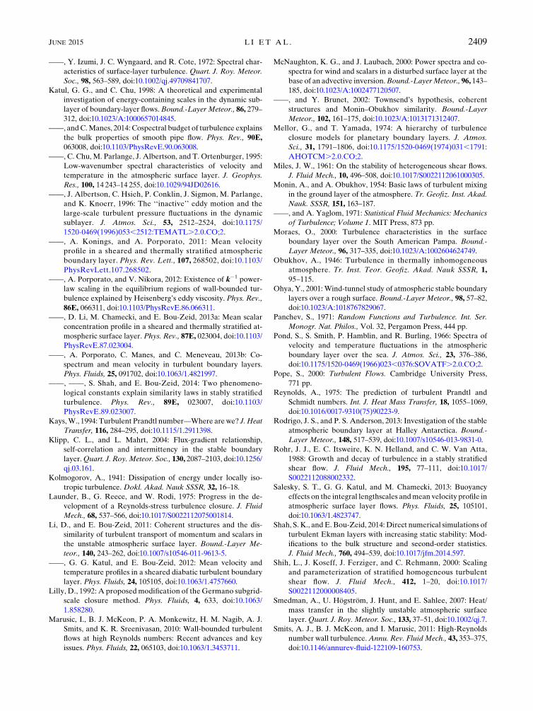
both Fww(K) and FTT(K), shown in Fig. 1, that reflect

observed scaling exponents in the ASL reported from

long-term field experiments (Kader and Yaglom 1991).

FIG. 1. The assumed shapes of (a) the vertical velocity and (b) the

air temperature spectra as a function of wavenumber K for near-

neutral and stable conditions (solid lines) and free-convective

conditions (dashed lines). When K.Ka, the spectra under near-

neutral and free-convective conditions overlap. The transition

wavenumbers Kd and Ka are indicated by the dashed–dotted lines,

and they can be different for Fww(K) andFTT(K), as denoted by the

subscripts w and T, respectively.

2398 JOURNAL OF THE ATMOSPHER IC SC IENCES VOLUME 72

Both Fww(K) and FTT(K) follow the expected Kolmo-

gorov 25/3 power-law scaling at sufficiently large

wavenumber (Kolmogorov 1941). The 25/3 scaling

commences from Kd under free-convective conditions

(z/2‘) but starts fromKa ’ 1/z under neutral and stable

conditions.A21 power-law scaling is allowed to exist over a

range of lowwavenumbers (fromKd toKa) forFTT(K), but

not for Fww(K) under near-neutral and stable conditions to

explore the impact of thepossibleoccurrenceof a21 scaling

in FTT(K), as suggested by several ASL experiments re-

ported elsewhere (Kader and Yaglom 1991; Katul et al.

1995; Katul and Chu 1998; Li et al. 2015, manuscript

submitted to Bound.-Layer Meteor.). Both spectra are

assumed to become invariant with K when K,Kd to

accommodate finite energy associated with very-large-

scale and super structures recently reported in laboratory

and ASL turbulence (Guala et al. 2010; Hutchins et al.

2012) and reviewed elsewhere (Marusic et al. 2010; Smits

et al. 2011). Hence, as a compromise between realistic

spectral shapes in the ASL and the need for maximum

simplicity in analytical tractability, the following idealized

forms for Fww(K) and FTT(K) are assumed:

Fww(K)5

8>><>>:

Cww1K2a

1 , for K,Kd,w

Cww2K2a

2 , for Kd,w ,K,Ka,w

Cww3K2a

3 , for K.Ka,w

and

FTT(K)5

8>><>>:

CTT1K2g

1 , for K,Kd,T

CTT2K2g

2 , for Kd,T ,K,Ka,T

CTT3K2g

3 , for K.Ka,T

As can be seen from Fig. 1, a1 5 0, g1 5 0, and

a3 5 g3 5 5/3.Under neutral and stable conditions,a2 5 0

and g2 5 1, while a2 5 g2 5 5/3 under free-convective

conditions. An interpolation a2 5 5/3[12 exp(5z)] is

used to cover the whole range of z# 0 so that a2 satisfies

both the neutral and the free-convective limits. Simi-

larly, g2 5 2/3[12 exp(5z)]1 1 is used when z# 0. As

such, the possible existence of 21 exponent in air tem-

perature spectra is restricted to be within a limited range

of z (i.e., under near-neutral conditions) when z, 0, as

reported in previous ASL experiments (Kader and

Yaglom 1991; Katul et al. 1995).

The values of Cww3and CTT3

can be determined from

Kolmogorov’s theory (Kolmogorov 1941) for the in-

ertial subrange: Cww35Co«

2/3 and CTT35CTNT«

21/3,

where Co is defined above and CT is the Kolmogorov–

Obukhov–Corrsin phenomenological constant. For a

one-dimensional-wavenumber interpretation, their values

are Co 5 0:65 and CT 5 0:8 (Ishihara et al. 2002; Chung

and Matheou 2012). The parameter « is the mean turbu-

lent kinetic energy dissipation rate, and NT is the mean

temperature variance dissipation rate. The values ofCww2,

Cww1,CTT2

, andCTT1are then determined from continuity

constraints on the spectra (e.g., Cww3K2a3

a,w 5Cww2K2a2

a,w

and Cww2K2a2

d,w 5Cww1K2a1

d,w ).

It is to be noted that the turbulent kinetic energy in the

vertical direction (TKEw) and the turbulent potential

energy (TPE) can be linked to Fww(K) and FTT(K)

(Zilitinkevich et al. 2007, 2008, 2013; Li et al. 2015,

manuscript submitted to Bound.-Layer Meteor.) using

TKEw 51

2

ð‘0Fww(K) dK and (26)

TPE51

2

b2

N2

ð‘0FTT(K) dK . (27)

Hence, specifying Fww(K) and FTT(K) is analogous to

specifying the vertical kinetic and potential energy dis-

tributions of turbulent eddies at each K. This provides a

clear connection between the proposed cospectral budget

model here and the energy- and flux-budget (EFB) tur-

bulence closure approach proposed by Zilitinkevich et al.

(2007, 2008, 2013), since TKEw/TPE was shown to be a

significant parameter in the EFB model.

e. The integration constants E1 and E2

Besides the spectral shapes of Fww(K) and FTT(K), the

integration constants (i.e.,E1 andE2) are also required to

evaluate Fuw(K) and FwT(K). Katul et al. (2013a) as-

sumed that ›FwT(K)/›K becomes zero when K5Ka.

As a result, the flux transfer term in the cospectral budget

of heat flux affectsfh only by a constant that is dependent

on ATT /AT . In our study, the integration constants (i.e.,

E1 and E2) are simply assumed to be zero. This is sup-

ported by experiments and DNS that reported 27/3

power-law scalings in the inertial subrange of momentum

and heat flux cospectra (Kaimal and Finnigan 1994; Pope

2000). Note, Eqs. (24) and (25) yield 27/3 scaling in the

inertial subrange of Fuw(K) and FwT(K), respectively,

when E1 5 0 and E2 5 0 are assumed, given a5 5/3 and

g5 5/3 in the inertial subrange. It is pointed out here that

the impact of flux transfer terms is not completely elim-

inated by doing so since the other terms on the right-hand

side of Eqs. (24) and (25) are still affected by flux transfer

terms. However, the impact of the flux transfer terms on

the anomalous scalings in the inertial subrange of mo-

mentum and heat flux cospectra are excluded when set-

ting E1 5 0 and E2 5 0.

3. Results

Using the idealized spectral shapes of Fww(K) and

FTT(K) and the assumption of E1 5E2 5 0, Eqs. (5) and

(6) can now be evaluated:

JUNE 2015 L I E T AL . 2399

u0w0 5ð‘0Fuw(K) dK5 f1D2Co«

2/3 and (28)

w0T 05ð‘0FwT(K) dK5 g1D4Co«

2/31 g2D5CTNT«21/3

5 g1D4Co«2/3Q .

(29)

Again, for maximum simplicity, local balances between

production and dissipation terms in the TKE and in the

temperature variance budgets are assumed to yield

(Katul et al. 2014; Li et al. 2015, manuscript submitted to

Bound.-Layer Meteor.):

Prt 52u0w0/S2w0T 0/G

5ATT(12CIU)

AUU(12CIT)

f1g1

1

Q, (30)

where

Q5 121

12CIT

CT

Co

g2g1

z

(fm 2 z), (31)

f151

(2a12 2/31D1)(2a11 1/3)K

2a211/3

d,w Ka22a

3a,w 1

1

(2a22 2/31D1)(2a21 1/3)(K

2a311/3

a,w 2K2a

211/3

d,w Ka22a

3a,w )

11

(2a32 2/31D1)(2a3 1 1/3)(2K

2a311/3

a,w ) ,

(32)

g151

(2a12 2/31D3)(2a11 1/3)K

2a211/3

d,w Ka22a

3a,w 1

1

(2a22 2/31D3)(2a21 1/3)(K

2a311/3

a,w 2K2a

211/3

d,w Ka22a

3a,w )

11

(2a32 2/31D3)(2a31 1/3)(2K

2a311/3

a,w ), and

(33)

g251

(2g12 2/31D3)(2g11 1/3)K

2g211/3

d,T Kg22g

3

a,T 11

(2g22 2/31D3)(2g21 1/3)(K

2g311/3

a,T 2K2g

211/3

d,T Kg22g

3

a,T )

11

(2g32 2/31D3)(2g31 1/3)(2K

2g311/3

a,T ) .

(34)

To ensure a downgradient sensible heat flux,Q. 0. The

parameters f1, g1, and g2 encode the shape functions of the

vertical velocity and temperature spectra. When z5 0

(i.e., under neutral conditions), Prt (denoted as Prt,neu)

becomes

Prt,neu5ATT(12CIU)

AUU(12CIT)

f1g1

. (35)

The departure of Prt,neu from unity, as predicted from

earlier theories (Mellor and Yamada 1974; Yamada

1975; Reynolds 1975; Yakhot et al. 1987; Zilitinkevich

et al. 2008, 2013) and many experiments and simulations

(Businger et al. 1971; Högström 1988; Kays 1994) can

now be critically examined. The main mechanisms that

introduce such departures are ATT 6¼ AUU , CIU 6¼ CIT ,

and f1 6¼ g1. As shown later, inequality between f1 and

g1 is primarily due to the inequality between ATT /AT

and AUU /AU . Consequently, inequality in the Rotta

constants, isotropization constants, and constants in

flux transfer terms between momentum and heat lead

to Prt,neu different from unity. Naturally, the assumed

balances between production and dissipation in the

turbulent kinetic energy and temperature variance

budgets also introduce further uncertainties. The evi-

dence in the literature thus far seems to be in support of

such approximations for unstable conditions when data

are conditioned for stationarity and planar homoge-

neity in the absence of subsidence (Hsieh and Katul

1997; Charuchittipan and Wilson 2009; Salesky et al.

2013), but for stable conditions, the emerging picture is

far less clear (Salesky et al. 2013). Moreover, most ASL

data tend to be infected by high-intensity turbulent

flow conditions at the very stable and near-convective

conditions, thereby complicating the use of Taylor’s

frozen turbulence hypothesis to infer dissipation rates

from structure functions or spectra.

From Eq. (30), Prt can also be expressed as Pr21t 5

Pr21t,neuQ, where Q represents the additional effects of

2400 JOURNAL OF THE ATMOSPHER IC SC IENCES VOLUME 72

stability on the turbulent Prandtl number separate from

those expected in near-neutral conditions. Denoting v1 5[1/(12CIT)](CT /Co)(g2/g1), Eq. (30) is recast as follows:

Pr21t 5Pr21

t,neu

"12v1

z

(fm 2 z)

#. (36)

Assuming that the stability correction function fm is

given by its Businger–Dyer form (Businger et al. 1971), a

form shown to be reasonable from recent multilevel

ASL experiments (Salesky et al. 2013), the dependence

of Prt on z is then primarily controlled by v1: namely, by

the ratio of the Kolmogorov to the Kolmogorov–

Obukhov–Corrsin phenomenological constants (CT /CO);

a constant associated with isotropization of the produc-

tion (CIT), the value of which can be determined from

rapid distortion theory in homogeneous turbulence

(53/5); and the ratio of g2/g1 encoding differences in

the spectral shapes of vertical velocity and air tempera-

ture. The near-universal values of the Kolmogorov

and the Kolmogorov–Obukhov–Corrsin phenomeno-

logical constants have been investigated extensively

(Sreenivasan 1995, 1996; Yeung and Zhou 1997). The

dependence of the Prt–z relation on the ratio of two

constants suggests that a possible universal Prt–z

relation (or Prt–Rg, where Rg is the gradient Richard-

son number; see below) may be inherited from the

Kolmogorov cascade in the inertial subrange, which is

consistent with recent literature demonstrating that

there are strong linkages between macroscopic fea-

tures in the logarithmic region of wall-bounded tur-

bulent flows and the Kolmogorov scaling (Gioia et al.

2010; Katul et al. 2013a, 2014, 2013b; Li et al. 2012;

Zúñiga Zamalloa et al. 2014; Katul and Manes 2014).

In addition, the fact that the Prt–z relation depends on

the ratio of CT /CO (basic constants associated with

spectral shapes of temperature and velocity) suggests

that both TPE and TKEw are important energetics in

the ASL, consistent with the EFBmodel (Zilitinkevich

et al. 2007, 2008, 2013). To illustrate this point further,

assuming the 21 scaling is absent in air temperature

spectra under neutral and stable conditions (see

Fig. 1), CT /CO is related to the ratio of TPE and TKEw

through

TPE

TKEw

5CT

Co

Rf

12Rf

. (37)

Interestingly, Rf at which the vertical turbulent kinetic en-

ergy is balanced by the turbulent potential energy is

Rf 5 (11CT /CO)21 ’ 0:45. This constraint on Rf (,0:45)

is much stronger than Rf imposed from TKE balance

considerations alone [i.e., «52w0u0S(12Rf ). 0] that

yield Rf , 1. However, this constraint on Rf (,0:45) is

not the most severe, as discussed next.

In addition to z, Rf and Rg are also widely used to

indicate the thermal stratification or the stability effect

in the ASL. Using Rf 5 z/fm, Prt can be formulated as a

function of Rf :

Pr21t 5Pr21

t,neu

2412v1

Rf

(12Rf )

35 . (38)

Given that the Prt 5Rg/Rf , Prt can be readily expressed

as a function of Rg, as follows:

Pr21t 5Pr21

t,neu

266411v2Rg2

ffiffiffiffiffiffiffiffiffiffiffiffiffiffiffiffiffiffiffiffiffiffiffiffiffiffiffiffiffiffiffiffiffiffiffiffiffiffiffiffiffiffiffiffiffiffiffi24Rg1 (212v2Rg)

2q

2Rg

3775 ,

(39)

where v2 5v1 1 1. The flux Richardson number is also

readily related to Rg through

Rf 5Pr21t,neu

266411v2Rg2

ffiffiffiffiffiffiffiffiffiffiffiffiffiffiffiffiffiffiffiffiffiffiffiffiffiffiffiffiffiffiffiffiffiffiffiffiffiffiffiffiffiffiffiffiffiffiffi24Rg1 (212v2Rg)

2q

2

3775 .

(40)

An interesting outcome of Eq. (40) is that Rf is limited

by some threshold or the ‘‘maximum flux Richardson

number’’ Rfm as Rg increases. The physical meaning

of this maximum flux Richardson number is that

Rf cannot increase infinitely under stable conditions

as Rg increases (Galperin et al. 2007). The gradient

Richardson number can be viewed as an external var-

iable that characterizes the mean flow; as a result, the

increase of Rg is not limited by the internal turbulence

state (Zilitinkevich et al. 2007). However, Rf depends on

the internal turbulence state and becomes saturated at

high stability, as already shown inKatul et al. (2014). This

maximum flux Richardson number can be inferred from

Eq. (38), given that the sensible heat flux is downgradient

(hence Q. 0 and Prt . 0) and Rf , 1 so that

Rfm51

v1 1 15

1

v2

. (41)

When AU 5AT 5 1:8, CIU 5CIT 5 3/5, and g2 5 g1, the

value of Rfm is 0.25, which is in agreement with the

values of Rfm reported in the literature (0.2–0.25). It is

pointed out here that Rfm should not be equated to the

‘‘critical gradient Richardson number’’Rgc inferred from

the classic Miles–Howard theory. This aforementioned

JUNE 2015 L I E T AL . 2401

theory yields a prediction of a critical Rg 5 0:25 associ-

ated with instability of a laminar boundary layer (Miles

1961; Howard 1961). The critical gradient Richardson

number of the Miles–Howard theory was assumed to

represent a critical Richardson number in some turbulent

studies, though this representation has been questioned

(Monin and Yaglom 1971). The concept of the critical

gradient Richardson number characterizing a laminar–

turbulent transition is not applicable to a laminarization

of a turbulent ASL, as discussed elsewhere (Galperin

et al. 2007; Zilitinkevich et al. 2007). Different from a

critical gradient Richardson number of the Miles–

Howard theory, the maximum flux Richardson number

is used to indicate a saturation value ofRf with increasing

Rg in turbulent flows. We note that Rfm has also been

labeled as a ‘‘critical’’ Richardson number in some other

studies (Yamada 1975; Grachev et al. 2013), but this label

is not linked with theMiles–Howard theory (even though

the maximum flux Richardson number value is close to

0.25). To avoid ambiguity in nomenclature, this saturated

value in a turbulent ASL is labeled as the maximum flux

Richardson number. The implications of this Rfm in the

cospectral budget framework are explained later. In ad-

dition, how the value of Rfm is influenced by the possible

existence of21 scaling in air temperature spectra and the

flux transfer terms are also explored.

a. Evaluation of modeled Prt from proposedcospectral budgets

Previous studies demonstrated the utility of the cospec-

tral budgets in reproducing variations of Pr21t /Pr21

t,neu for

stable conditions when g2 5 g1 (Katul et al. 2014).

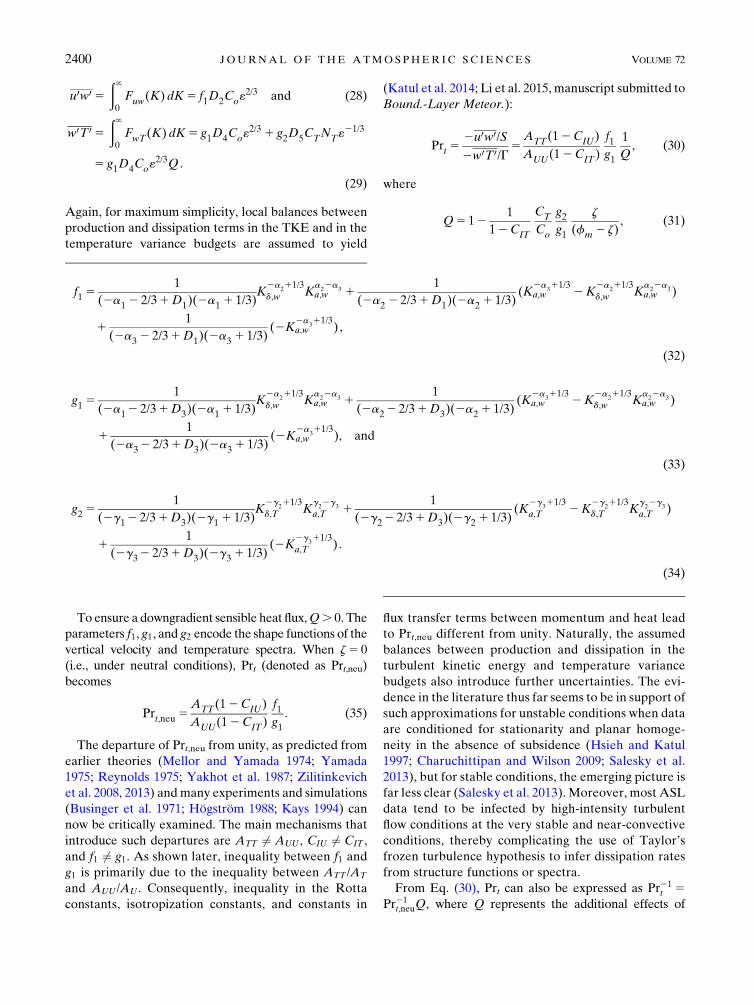
Figure 2 shows modeled Pr21t /Pr21

t,neu or Q using the

cospectral budgets whenKd,T 5Ka,T [i.e., the21 power-

law scaling is absent in FTT(K) at low K] for unstable

conditions. Since the ratio of g2/g1 is also dependent on

the inequality between Kd,w and Ka,w under unstable

conditions, results with Kd,w 5Ka,w (the black dashed

line) andKd,w 5 0:8Ka,w (the black line) are both shown in

Fig. 2. These predictions are compared to data frommany

field experiments. It is clear that the cospectral budgets

method captures the general variation of Pr21t /Pr21

t,neu with

z under unstable conditions reported in many experi-

ments. The model with Kd,w 5 0:8Ka,w (black line) re-

duces Prt under very unstable conditions and better agrees

with experiments, suggesting the need for a further ex-

tension of the 25/3 scaling in Fww(K) as instability in-

creases, which is in agreement with spectral shapes

reported elsewhere for forced and free convection in the

ASL (Kader and Yaglom 1991).

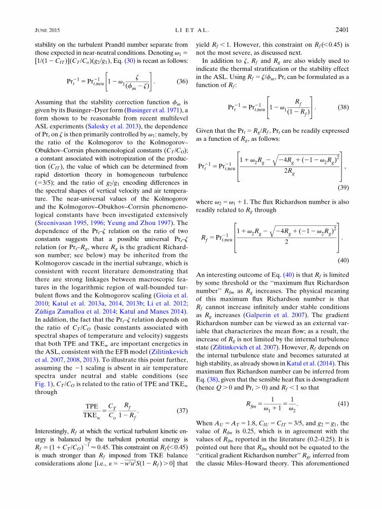
The cospectral budgets model is further compared

against theEFB turbulence closuremodel developed for

stable conditions (Zilitinkevich et al. 2007, 2008, 2013)

in Fig. 3. The Prt–Rg relation instead of the Prt– z re-

lation is examined under stable conditions to avoid self-

correlation between Prt and z or Rf reported in the

experiments (Klipp and Mahrt 2004; Esau and Grachev

2007; Grachev et al. 2007; Anderson 2009; Rodrigo and

Anderson 2013). Zilitinkevich et al. (2013) pointed out

that under stable conditions, Prt increases as Rg in-

creases and has the asymptote Prt /Rg/Rfm when

Rg /‘. Figure 3 shows that the cospectral budgets

model reproduces the increasing trend of Prt (or the

FIG. 2. Comparison between modeled Pr21t /Pr21

t,neu from the co-

spectral budgetswhenKd,T 5Ka,T 5Ka,w (i.e., no21 power scaling in

the air temperature spectra) and Kd,w 5 0:8Ka,w (black solid line) or

Kd,w 5Ka,w (black dashed line) with experiments and simulations for

a wide range of unstable conditions. The inequality betweenKd,w and

Ka,w only affects the unstable part, since only under unstable condi-

tions is the scaling betweenKd,w andKa,w nonzero.Data are fromASL

field experiments8 inKansas (Businger et al. 1971);P inKerang and

Hay,Australia (Brutsaert 1982);9 in Pampa, Brazil (Moraes 2000);Din Tsimlyansk, Russia (Kader and Yaglom 1990); and u in Gotland

Island, Sweden (Smedman et al. 2007).

FIG. 3. Comparison between modeled Pr21t /Pr21

t,neu from the co-

spectral budgets model and from the EFB model with experiments

and simulations for a wide range of stable conditions. Data are

from numerical simulations, including DNS and LES, laboratory,

and field experiments: 8 for DNS (Shih et al. 2000), 9 for DNS

(Stretch et al. 2010),P for DNS (Chung andMatheou 2012), D for

LES (Esau and Grachev 2007), ) for LES (Andren 1995), 1 for

water channel (Rohr et al. 1988), u for wind tunnel (Webster

1964), s for wind tunnel (Ohya 2001), and * for SHEBA field

experiment (Grachev et al. 2007).

2402 JOURNAL OF THE ATMOSPHER IC SC IENCES VOLUME 72

decreasing trend of Pr21t ) as Rg increases, which is also

consistent with other theoretical work using the quasi-

normal scale elimination theory (Galperin et al. 2007).

Moreover, as Rg/‘, Prt is almost a linear function of

Rg, the slope of which is also similar to the slope from the

EFBmodel (not shown here but similar slopes in the two

models can be inferred fromFig. 3), implying that theRfm

values are similar in both the cospectral budgets model

and the EFB model. It is, however, noted here that

Rfm5 0:25 was preset in the EFB model, while it is an

outcome of model calculations in the cospectral budgets.

b. The impact of possible 21 scaling in airtemperature spectra on Prt

The 21 power-law scaling has been reported in sev-

eral ASL experiments for the spectra of streamwise

velocity, pressure, and skin and air temperature, espe-

cially for near-neutral conditions (Kader and Yaglom

1991; Katul et al. 1995, 1996; Katul and Chu 1998;

McNaughton and Laubach 2000; Katul et al. 2012;

Banerjee and Katul 2013; Katul et al. 2013b). A recent

study also showed that a21 power-law scaling existed in

air temperature spectra for near-neutral to mildly stable

conditions over lakes and glaciers (Li et al. 2015, man-

uscript submitted to Bound.-Layer Meteor.). However,

the universal character of the 21 scaling in air temper-

ature spectra remains questionable. For example, early

experiments by Pond and coworkers over sea do report a

K21 scaling in their longitudinal velocity spectra but not

in their air temperature (or vertical velocity) spectra

(Pond et al. 1966). Likewise, measured air temperature

spectra in a stableASL reported byGrachev et al. (2013)

also do not support an extensive 21 power-law scaling.

Hence, an exploration of how the21 power-law scaling

in air temperature spectra may modify Prt is warranted.

The possible existence of 21 power law in the air tem-

perature spectra can be represented here by the in-

equality between Kd,T and Ka,T . As can be seen from

Eqs. (35), (32), and (33), the possible existence of 21

scaling has no impact on the Prt,neu but affects the ratio

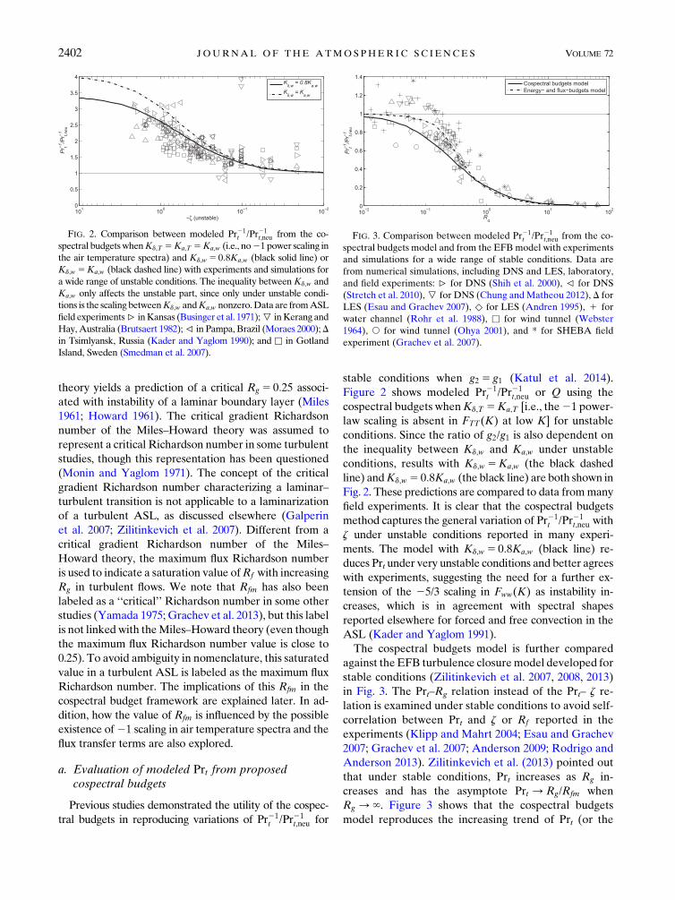
g2/g1 and, thus, Q. Figure 4 shows the variations of

Pr21t /Pr21

t,neu as functions of z, Rg, and Rf for three cases

(Kd,T /Ka,T 5 1, Kd,T /Ka,T 5 0:5, and Kd,T /Ka,T 5 0:2).

First, Pr21t /Pr21

t,neu when Kd,T 5Ka,T is examined. It is

clear that the Pr21t /Pr21

t,neu increases as the atmosphere

becomes more unstable, while it decreases as the atmo-

sphere becomes more stable, implying that sensible heat is

transferredmore efficiently under unstable conditions and

less efficiently under stable conditions when compared to

momentum. The relation between Pr21t /Pr21

t,neu and z is

almost identical to that between Pr21t /Pr21

t,neu and Rg,

which is in agreement with Businger (1988) regarding a

near correspondence between z and Rg. A difference is

observed in the relation between Prt and Rf (Fig. 4c).

Unlike z and Rg, which may increase to very large values

under stable conditions, Rf is limited by Rfm. Again, the

numerical value of this Rfm is a direct outcome of the

cospectral budget model, as demonstrated by Eq. (41),

which is also in agreement with the values ofRfm reported

in the literature and assumed in the EFB model.

Figure 4 further shows how variations of Pr21t /Pr21

t,neu

with z, Rg, and Rf are modified by the possible existence

of a 21 scaling in the air temperature spectra. To sim-

plify the analysis, ATT /AT 5 1 is assumed here; but, as

shown later, the exact value ofATT /AT only changes the

stability impact on Pr21t /Pr21

t,neu in a minor way. It is clear

that Pr21t is increased significantly when z, 0 but de-

creased when z. 0 because of the possible existence

of a21 power-law scaling. This result implies that when

such a 21 power-law scaling is primarily observed in

the air temperature spectra, Prt becomes more sensitive

to the atmospheric stability effect. This may be because

of the existence of large-scale, inactive eddies under

FIG. 4. Pr21t /Pr21

t,neu as a function of (a) z5 z/L, (b) Rg, and (c) Rf

when the21 scaling law is prevalent in the spectra of air temperature.

Here,Kd,T canbe smaller thanKa,T . The inset in (c) further emphasizes

the results for stableASLconditions.Note thatATT /AT 5 1 is assumed

here, but other values of ATT /AT yield similar results.

JUNE 2015 L I E T AL . 2403

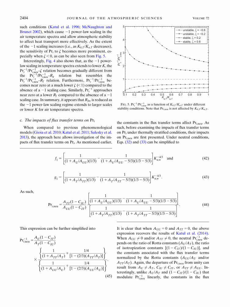
such conditions (Katul et al. 1996; McNaughton and

Brunet 2002), which cause 21 power-law scaling in the

air temperature spectra and allow atmospheric stability

to affect heat transport more effectively. As the extent

of the21 scaling increases (i.e., as Kd,T /Ka,T decreases),

the sensitivity of Prt to z becomes more prominent, es-

pecially when z, 0, as can be also seen from Fig. 5.

Interestingly, Fig. 4 also shows that, as the 21 power-

law scaling in temperature spectra extends to lowerK, the

Pr21t /Pr21

t,neu–z relation becomes gradually different from

the Pr21t /Pr21

t,neu–Rg relation but resembles the

Pr21t /Pr21

t,neu–Rf relation. Furthermore, Pr21t /Pr21

t,neu be-

comes near zero at a much lower z (,1) compared to the

absence of a 21 scaling case. Similarly, Pr21t approaches

near zero at a lower Rf compared to the absence of a21

scaling case. In summary, it appears thatRfm is reduced as

the21 power-law scaling regime extends to larger scales

or lower K for air temperature spectra.

c. The impacts of flux transfer terms on Prt

When compared to previous phenomenological

models (Gioia et al. 2010; Katul et al. 2011; Salesky et al.

2013), the approach here allows investigation of the im-

pacts of flux transfer terms on Prt. As mentioned earlier,

the constants in the flux transfer terms affect Prt,neu. As

such, before examining the impacts of flux transfer terms

on Prt under thermally stratified conditions, their impacts

on Prt,neu are first presented. Under neutral conditions,

Eqs. (32) and (33) can be simplified to

f15

"1

(11AU /AUU)(1/3)2

1

(11AU /AUU 2 5/3)(1/32 5/3)

#K24/3

a,w and (42)

g15

"1

(11AT /ATT)(1/3)2

1

(11AT /ATT2 5/3)(1/32 5/3)

#K24/3

a,w . (43)

As such,

Prt,neu5ATT(12CIU)

AUU(12CIT)

"1

(11AU /AUU)(1/3)2

1

(11AU /AUU 2 5/3)(1/32 5/3)

#"

1

(11AT /ATT)(1/3)2

1

(11AT /ATT2 5/3)(1/32 5/3)

# . (44)

This expression can be further simplified into

Pr21t,neu5

AU(12CIT)

AT(12CIU)

3

(1

(11ATT /AT)1

1/4

[12 (2/3)(ATT /AT)]

)(

1

(11AUU /AU)1

1/4

[12 (2/3)(AUU /AU)]

) .

(45)

It is clear that when AUU 5 0 and ATT 5 0, the above

expression recovers the results of Katul et al. (2014).

When AUU 6¼ 0 and/or ATT 6¼ 0, the neutral Pr21t,neu de-

pends on the ratio of Rotta constants (AU /AT), the ratio

of isotropization constants [(12CIT)/(12CIU)], and

the constants associated with the flux transfer terms

normalized by the Rotta constants (AUU /AU and/or

ATT /AT). Again, the departure of Prt,neu from unity can

result from AU 6¼ AT , CIU 6¼ CIT , or ATT 6¼ AUU . In-

terestingly, unlike AU /AT and (12CIT)/(12CIU) that

modulate Pr21t,neu linearly, the constants in the flux

FIG. 5. Pr21t /Pr21

t,neu as a function of Kd,T /Ka,T under different

stability conditions. Note that Prt,neu is not affected by Kd,T /Ka,T .

2404 JOURNAL OF THE ATMOSPHER IC SC IENCES VOLUME 72

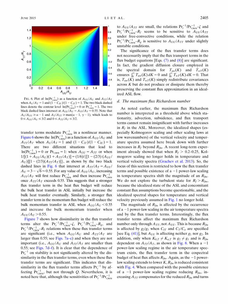
transfer terms modulate Pr21t,neu in a nonlinear manner.

Figure 6 shows the ln(Pr21t,neu) as a function ofAUU /AU and

ATT /AT when AU /AT 5 1 and (12CIT)/(12CIU)5 1.

There are two different situations that lead to

ln(Pr21t,neu)5 0 or Prt,neu 5 1: when AUU 5ATT or when

1/[(11AUU /AU)(11ATT /AT)]5 (1/6)/f[12 (2/3) (AUU /

AU)][12 (2/3)(ATT /AT)]g, as shown by the two black

dashed lines in Fig. 6 that intersect at ATT /AT 5AUU /

AU 532ffiffiffi6

p’0:55. For any value ofAUU /AU , increasing

ATT /AT will first reduce Pr21t,neu and then increase Pr21

t,neu

once ATT /AT exceeds 0.55. This suggests that a stronger

flux transfer term in the heat flux budget will reduce

the bulk heat transfer in ASL initially but increase the

bulk heat transfer eventually. Similarly, a stronger flux

transfer term in the momentum flux budget will reduce the

bulk momentum transfer in ASL when AUU /AU ,0:55

and increase the bulk momentum transfer when

AUU /AU .0:55.

Figure 7 shows how dissimilarity in the flux transfer

terms alter the Pr21t /Pr21

t,neu–z, Pr21t /Pr21

t,neu–Rg, and

Pr21t /Pr21

t,neu–Rf relations when these flux transfer terms

are significant (i.e., when AUU /AU and ATT /AT are

larger than 0.55; see Figs. 7a–c) and when they are not

important (i.e., AUU /AU and ATT /AT are smaller than

0.55; see Figs. 7d–f). It is clear that the dependence of

Pr21t on stability is not significantly altered by the dis-

similarity in the flux transfer terms, even when these flux

transfer terms are significant. This indicates that dis-

similarity in the flux transfer terms affects Pr21t by af-

fecting Pr21t,neu, but not through Q. Nevertheless, it is

noted here that, although the sensitivities of Pr21t /Pr21

t,neu

to AUU /ATT are small, the relations Pr21t /Pr21

t,neu–z and

Pr21t /Pr21

t,neu–Rf seems to be sensitive to AUU /ATT

under free-convective conditions, while the relation

Pr21t /Pr21

t,neu–Rg is sensitive to AUU /ATT under slightly

unstable conditions.

The significance of the flux transfer terms does

not necessarily imply that the flux transport terms in the

flux budget equations [Eqs. (7) and (8)] are significant.

In fact, the gradient diffusion closure employed in

the spectral domain for Tuw(K) and TwT(K)

ensuresÐ ‘0 Tuw(K) dK5 0 and

Ð ‘0 TwT(K) dK5 0. That

is, Tuw(K) and TwT(K) simply redistribute covariances

across K but do not produce or dissipate them thereby

preserving the constant flux approximation in an ideal-

ized ASL flow.

d. The maximum flux Richardson number

As noted earlier, the maximum flux Richardson

number is interpreted as a threshold above which sta-

tionarity, advection, subsidence, and flux transport

terms cannot remain insignificant with further increases

in Rf in the ASL. Moreover, the idealized shapes (es-

pecially Kolmogorov scaling and other scaling laws at

low wavenumbers) of the vertical velocity and temper-

ature spectra assumed here break down with further

increases in Rf beyond Rfm. A recent long-term exper-

iment already showed that when Rf . 0.2–0.25, Kol-

mogorov scaling no longer holds in temperature and

vertical velocity spectra (Grachev et al. 2013). So, the

focus of this section is restricted to how the flux transfer

terms and possible existence of a 21 power-law scaling

in temperature spectra shift the magnitude of an Rfm.

We do not explore the turbulent state for Rf .Rfm,

because the idealized state of the ASL and concomitant

constant flux assumptions become questionable, and the

idealized spectral shapes for temperature and vertical

velocity previously assumed in Fig. 1 no longer hold.

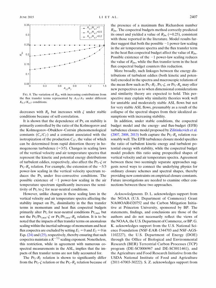
The magnitude of Rfm is affected by the occurrence

of a21 power-law scaling in the air temperature spectra

and by the flux transfer terms. Interestingly, the flux

transfer terms affect the maximum flux Richardson

number only throughATT , notAUU . This is because Rfm

is affected by g2/g1 when CIT and CT /Co are specified

[see Eq. (41)], but AUU is affecting neither g1 nor g2. In

addition, only when Kd,T 6¼ Ka,T is g2 6¼ g1 and is Rfm

dependent on ATT /AT , as shown in Fig. 8. When a 21

power-law scaling regime in the air temperature spec-

trum exists, the flux transfer term in the cospectral

budget of heat flux affects Rfm. Again, as the21 power-

law scaling extends to lowerK,Rfm is reduced consistent

with Fig. 4. When compared with the possible existence

of a 21 power-law scaling regime reducing Rfm, in-

creasingATT compensates for the reducedRfm and turns

FIG. 6. Plot of ln(Pr21t,neu) as a function of AUU /AU and ATT /AT

whenAU /AT 5 1 and (12CIU)/(12CIT)5 1. The two black dashed

lines denote the contour level ln(Pr21t,neu)5 0 or Pr21

t,neu 5 1. The two

black dashed lines intersect at AUU /AU 5ATT /AT ’ 0:55. Note that

AU /AUU $a2 1 and AT /ATT $max(a2 1, g2 1), which leads to

0#AUU /AU # 3/2 and 0#ATT /AT # 3/2.

JUNE 2015 L I E T AL . 2405

it back to its value when Kd,T 5Ka,T . Hence, it can be

conjectured that the flux transfer term in the heat flux

budget mediates the impact of the21 power-law scaling

in air temperature spectra on Rfm.

4. Conclusions and discussion

A recently proposed cospectral budget method that

links kinetic energy of eddies in the vertical direction via

Fww(K) and their potential energy via FTT(K) to mac-

roscopic relations, such as Prt–z (or Prt–Rg), is general-

ized here to accommodate extensions of the 25/3

power-law scaling in both vertical velocity and air tem-

perature spectra for free-convective conditions, the

possible existence of 21 power-law scaling in air tem-

perature spectra under near-neutral and mildly stable

conditions, and the existence of finite flux transfer terms.

The generalized model reproduces the Prt–z relation

under unstable conditions and the Prt–Rg relation under

stable conditions reported in many experiments and

simulations. Pr21t is shown to decrease with z or Rg,

implying that heat is transferred less efficiently than

momentum as stability increases. This does not contra-

dict several experimental studies showing that Pr21t

FIG. 7. Pr21t /Pr21

t,neu as a function of (a),(d) z5 z/L; (b),(e) Rg; and (c),(f) Rf when dissimilarity exists between the

flux transfer terms in momentum and heat flux cospectral budgets. Kd,T 5Ka,T is assumed here, but other values of

Kd,T 5Ka,T also yield similar results, except that the maximum flux Richardson number is altered by the inequality

between Kd,T and Ka,T , as in Fig. 8. In (a)–(c), AUU /AU 5 1. 0:55 is used, while in (d)–(f), AUU /AU 5 0:3, 0:55

is used.

2406 JOURNAL OF THE ATMOSPHER IC SC IENCES VOLUME 72

decreases with Rg but increases with z under stable

conditions because of self-correlation.

It is shown that the dependence of Prt on stability is

primarily controlled by the ratio of the Kolmogorov and

the Kolmogorov–Obukhov–Corrsin phenomenological

constants (Co/CT) and a constant associated with the

isotropization of the production CIT , the value of which

can be determined from rapid distortion theory in ho-

mogeneous turbulence (53/5). Changes in scaling laws

of the vertical velocity and air temperature spectra that

represent the kinetic and potential energy distributions

of turbulent eddies, respectively, also affect the Prt–z or

Prt–Rg relation. For example, the extension of the 25/3

power-law scaling in the vertical velocity spectrum re-

duces the Prt under free-convective conditions. The

possible existence of 21 power-law scaling in the air

temperature spectrum significantly increases the sensi-

tivity of Prt to z for near-neutral conditions.

However, unlike changes in these scaling laws in the

vertical velocity and air temperature spectra affecting the

stability impact on Prt, dissimilarity in the flux transfer

terms in momentum and heat flux cospectral budgets

primarily alter Prt for near-neutral conditions Prt,neu but

not the Prt/Prt,neu–z or Prt/Prt,neu–Rg relation. It is to be

noted that the impacts of flux transfer terms on anomalous

scalingwithin the inertial subrange ofmomentumandheat

flux cospectra are excluded by settingE1 5 0 andE2 5 0 in

Eqs. (24) and (25), respectively, thereby ensuring that such

cospectramaintain aK27/3 scaling exponent. Nonetheless,

this restriction, while in agreement with numerous co-

spectral measurements in the ASL, implies that the im-

pacts of flux transfer terms are not fully accounted for.

The Prt–Rf relation is shown to significantly differ

from the Prt–z relation or the Prt–Rg relation because of

the presence of a maximum flux Richardson number

Rfm. The cospectral budgets method correctly predicted

its onset and yielded a value of Rfm (’0.25), consistent

with those reported in the literature. Model results fur-

ther suggest that both the possible21 power-law scaling

in the air temperature spectra and the flux transfer term

in the heat flux cospectral budget affect the value ofRfm.

Possible existence of the 21 power-law scaling reduces

the value of Rfm, while the flux transfer term in the heat

flux cospectral budget counters this reduction.

More broadly, such linkages between the energy dis-

tributions of turbulent eddies (both kinetic and poten-

tial) encoded in the spectra andmacroscopic relations of

the mean flow such as Prt–Rf , Prt–z, or Prt–Rg may offer

new perspectives as to when dimensional considerations

and similarity theory are expected to hold. This per-

spective may explain why similarity theories work well

for unstable and moderately stable ASL flows but not

for very stable ASL flows, presumably as a result of the

collapse of the spectral shapes from their idealized as-

sumptions with increasing stability.

In addition, under stable conditions, the cospectral

budget model and the energy- and flux-budget (EFB)

turbulence closure model proposed by Zilitinkevich et al.

(2007, 2008, 2013) both capture the Prt–Rg relation rea-

sonablywell. TheEFB turbulence closuremodel specifies

the ratio of turbulent kinetic energy and turbulent po-

tential energy with stability, while the cospectral budget

model predicts this ratio using prespecified shapes of

vertical velocity and air temperature spectra. Agreement

between these two seemingly separate approaches sug-

gests novel ways to connect the underlying physics for

ordinary closure schemes and spectral shapes, thereby

providing new constraints on empirical closure constants.

Future investigations are needed to examine other con-

nections between these two approaches.

Acknowledgments. D. L. acknowledges support from

the NOAA (U.S. Department of Commerce) Grant

NA08OAR4320752 and the Carbon Mitigation Initia-

tive at Princeton University, sponsored by BP. The

statements, findings, and conclusions are those of the

authors and do not necessarily reflect the views of

theNOAA, theU.S.Department ofCommerce, orBP.G.

K. acknowledges support from the U.S. National Sci-

ence Foundation (NSF-EAR-1344703 and NSF-AGS-

1102227), the U.S. Department of Energy (DOE)

through the Office of Biological and Environmental

Research (BER) Terrestrial Carbon Processes (TCP)

program (DE-SC0006967 and DE-SC0011461), and

the Agriculture and Food Research Initiative from the

USDA National Institute of Food and Agriculture

(2011-67003-30222). S. Z. acknowledges support from

FIG. 8. The variation of Rfm with increasing contributions from

the flux transfer terms represented by ATT /AT under different

Kd,T /Ka,T conditions.

JUNE 2015 L I E T AL . 2407

the European Commission ERC-Ideas PoC Project

632295-INMOST (2014–15); the Academy of Finland

project ABBA, Contract 280700 (2014–17); the Rus-

sian Mega-grant Contract 11.G34.31.0048 (2011–15);

and the Russian Federal Program—Research and

Development on priority directions of development of

scientific–technological infrastructure of Russia for

2014–20, Contract 14.578.21.0033 (2014–16).

REFERENCES

Anderson, P. S., 2009:Measurement of Prandtl number as a function

of Richardson number avoiding self-correlation. Bound.-Layer

Meteor., 131, 345–362, doi:10.1007/s10546-009-9376-4.

Andren, A., 1995: The structure of stably stratified atmospheric

boundary layers: A large eddy simulation study.Quart. J. Roy.

Meteor. Soc., 121, 961–985, doi:10.1002/qj.49712152502.

Baldocchi, D., and Coauthors, 2001: FLUXNET: A new tool to

study the temporal and spatial variability of ecosystem-

scale carbon dioxide, water vapor, and energy flux densi-

ties. Bull. Amer. Meteor. Soc., 82, 2415–2434, doi:10.1175/

1520-0477(2001)082,2415:FANTTS.2.3.CO;2.

Banerjee, T., and G. Katul, 2013: Logarithmic scaling in the lon-

gitudinal velocity variance explained by a spectral budget.

Phys. Fluids, 25, 125106, doi:10.1063/1.4837876.Bodenschatz, E., S. P. Malinowski, R. A. Shaw, and F. Stratmann,

2010: Can we understand clouds without turbulence? Science,

327, 970–971, doi:10.1126/science.1185138.

Bos, W., and J. Bertoglio, 2007: Inertial range scaling of scalar flux

spectra in uniformly sheared turbulence. Phys. Fluids, 19,

025104, doi:10.1063/1.2565563.

——, H. Touil, L. Shao, and J. Bertogli, 2004: On the behavior of

the velocity-scalar cross correlation spectrum in the inertial

range. Phys. Fluids, 16, 3818–3823, doi:10.1063/1.1779229.Bou-Zeid, E., N. Vercauteren, M. Parlange, and C. Meneveau,

2008: Scale dependence of subgrid-scale model coefficients:

An a priori study. Phys. Fluids, 20, 115106, doi:10.1063/

1.2992192.

Brutsaert, W. B., 1982: Evaporation into the Atmosphere. Kluwer

Academic Publishers, 299 pp.

——, 2005: Hydrology: An Introduction. Cambridge University

Press, 605 pp.

Businger, J. A., 1988: A note on the Businger–Dyer profiles.

Bound.-Layer Meteor., 42, 145–151, doi:10.1007/BF00119880.

——, and A. M. Yaglom, 1971: Introduction to Obukhov’s paper

on ‘Turbulence in an atmosphere with a non-uniform

temperature.’ Bound.-Layer Meteor., 2, 3–6, doi:10.1007/

BF00718084.

——, J. C. Wyngaard, Y. Izumi, and E. F. Bradley, 1971: Flux-

profile relationships in the atmospheric surface layer. J.Atmos.

Sci., 28, 181–191, doi:10.1175/1520-0469(1971)028,0181:

FPRITA.2.0.CO;2.

Canuto, V. M., Y. Cheng, A. Howard, and I. Esau, 2008: Stably

stratified flows: A model with no Ri(cr). J. Atmos. Sci., 65,

2437–2447, doi:10.1175/2007JAS2470.1.

Cava,D., andG.Katul, 2012:On the scaling laws of the velocity-scalar

cospectra in the canopy sublayer above tall forests. Bound.-

Layer Meteor., 145, 351–367, doi:10.1007/s10546-012-9737-2.

Charuchittipan, D., and J. Wilson, 2009: Turbulent kinetic energy

dissipation in the surface layer. Bound.-Layer Meteor., 132,

193–204, doi:10.1007/s10546-009-9399-x.

Choi, K., and J. Lumley, 2001: The return to isotropy of homoge-

neous turbulence. J. Fluid Mech., 436, 59–84, doi:10.1017/

S002211200100386X.

Chung, D., and G. Matheou, 2012: Direct numerical simulation of

stationary homogeneous stratified sheared turbulence. J. Fluid

Mech., 696, 434–467, doi:10.1017/jfm.2012.59.

Corrsin, S., 1961: The reactant concentration spectrum in turbulent

mixing with a first-order reaction. J. Fluid Mech., 11, 407–416,

doi:10.1017/S0022112061000615.

Esau, I., and A. A. Grachev, 2007: Turbulent Prandtl number in

stably stratified atmospheric boundary layer: Intercomparison

between LES and SHEBA data. e-WindEng, 006, 1–17.

[Available online at http://ejournal.windeng.net/16/.]

Galperin, B., S. Sukoriansky, and P. S. Anderson, 2007: On the

critical Richardson number in stably stratified turbulence.

Atmos. Sci. Lett., 8, 65–69, doi:10.1002/asl.153.

Gioia, G., N. Guttenberg, N. Goldenfeld, and P. Chakraborty,

2010: Spectral theory of the turbulent mean-velocity

profile. Phys. Rev. Lett., 105, 184501, doi:10.1103/

PhysRevLett.105.184501.

Grachev, A., E. Andreas, C. Fairall, P. Guest, and P. G. Persson,

2007: On the turbulent Prandtl number in the stable atmo-

spheric boundary layer. Bound.-Layer Meteor., 125, 329–341,

doi:10.1007/s10546-007-9192-7.

——, ——, ——, ——, and ——, 2013: The critical Richardson

number and limits of applicability of local similarity theory in

the stable boundary layer. Bound.-Layer Meteor., 147, 51–82,

doi:10.1007/s10546-012-9771-0.

Guala, M., M. Metzger, and B.McKeon, 2010: Intermittency in the

atmospheric surface layer: Unresolved or slowly varying?

Physica D, 239, 1251–1257, doi:10.1016/j.physd.2009.10.010.Högström, U., 1988: Non-dimensional wind and temperature pro-

files in the atmospheric surface layer: A re-evaluation.

Bound.-Layer Meteor., 42, 55–78, doi:10.1007/BF00119875.Howard, L. N., 1961: Note on a paper of John W. Miles. J. Fluid

Mech., 10, 509–512, doi:10.1017/S0022112061000317.

Hsieh, C.-I., and G. G. Katul, 1997: Dissipation methods, Taylor’s

hypothesis, and stability correction functions in the atmo-

spheric surface layer. J. Geophys. Res., 102, 16 391–16 405,

doi:10.1029/97JD00200.

Hutchins, N., K. Chauhan, I. Marusic, J. Monty, and J. Klewicki,

2012: Towards reconciling the large-scale structure of turbulent

boundary layers in the atmosphere and laboratory. Bound.-

Layer Meteor., 145, 273–306, doi:10.1007/s10546-012-9735-4.Ishihara, T., K. Yoshida, andY. Kaneda, 2002: Anisotropic velocity

correlation spectrum at small scales in a homogeneous tur-

bulent shear flow. Phys. Rev. Lett., 88, 154501, doi:10.1103/

PhysRevLett.88.154501.

Kader, B. A., and A. M. Yaglom, 1990: Mean fields and fluctuation

moments in unstably stratified turbulent boundary layers.

J. Fluid Mech., 212, 637–662, doi:10.1017/S0022112090002129.——, and ——, 1991: Spectra and correlation functions of surface

layer atmospheric turbulence in unstable thermal stratifica-

tion. Turbulence and Coherent Structures, O. Metais and

M. Lesieur, Eds., Fluid Mechanics and Its Applications,

Vol. 2, Kluwer Academic Publishers, 387–412, doi:10.1007/

978-94-015-7904-9_24.

Kaimal, J. C., 1973: Turbulence spectra, length scales and structure

parameters in the stable surface layer. Bound.-Layer Meteor.,

4, 289–309, doi:10.1007/BF02265239.

——, and J. Finnigan, 1994: Atmospheric Boundary Layer Flows:

Their Structure and Measurement. Oxford University Press,

289 pp.

2408 JOURNAL OF THE ATMOSPHER IC SC IENCES VOLUME 72

——, Y. Izumi, J. C. Wyngaard, and R. Cote, 1972: Spectral char-

acteristics of surface-layer turbulence. Quart. J. Roy. Meteor.

Soc., 98, 563–589, doi:10.1002/qj.49709841707.

Katul, G. G., and C. Chu, 1998: A theoretical and experimental

investigation of energy-containing scales in the dynamic sub-

layer of boundary-layer flows. Bound.-Layer Meteor., 86, 279–

312, doi:10.1023/A:1000657014845.

——, andC.Manes, 2014: Cospectral budget of turbulence explains

the bulk properties of smooth pipe flow. Phys. Rev., 90E,

063008, doi:10.1103/PhysRevE.90.063008.

——, C. Chu, M. Parlange, J. Albertson, and T. Ortenburger, 1995:

Low-wavenumber spectral characteristics of velocity and

temperature in the atmospheric surface layer. J. Geophys.

Res., 100, 14 243–14 255, doi:10.1029/94JD02616.

——, J. Albertson, C. Hsieh, P. Conklin, J. Sigmon, M. Parlange,

and K. Knoerr, 1996: The ‘‘inactive’’ eddy motion and the

large-scale turbulent pressure fluctuations in the dynamic

sublayer. J. Atmos. Sci., 53, 2512–2524, doi:10.1175/

1520-0469(1996)053,2512:TEMATL.2.0.CO;2.

——, A. Konings, and A. Porporato, 2011: Mean velocity

profile in a sheared and thermally stratified atmospheric

boundary layer. Phys. Rev. Lett., 107, 268502, doi:10.1103/

PhysRevLett.107.268502.

——, A. Porporato, and V. Nikora, 2012: Existence of k21 power-

law scaling in the equilibrium regions of wall-bounded tur-

bulence explained by Heisenberg’s eddy viscosity. Phys. Rev.,

86E, 066311, doi:10.1103/PhysRevE.86.066311.

——, D. Li, M. Chamecki, and E. Bou-Zeid, 2013a: Mean scalar

concentration profile in a sheared and thermally stratified at-

mospheric surface layer. Phys. Rev., 87E, 023004, doi:10.1103/

PhysRevE.87.023004.

——, A. Porporato, C. Manes, and C. Meneveau, 2013b: Co-

spectrum and mean velocity in turbulent boundary layers.

Phys. Fluids, 25, 091702, doi:10.1063/1.4821997.——, ——, S. Shah, and E. Bou-Zeid, 2014: Two phenomeno-

logical constants explain similarity laws in stably stratified

turbulence. Phys. Rev., 89E, 023007, doi:10.1103/

PhysRevE.89.023007.

Kays,W., 1994: Turbulent Prandtl number—Where arewe? J. Heat

Transfer, 116, 284–295, doi:10.1115/1.2911398.

Klipp, C. L., and L. Mahrt, 2004: Flux-gradient relationship,

self-correlation and intermittency in the stable boundary

layer.Quart. J. Roy.Meteor. Soc., 130, 2087–2103, doi:10.1256/

qj.03.161.

Kolmogorov, A., 1941: Dissipation of energy under locally iso-

tropic turbulence. Dokl. Akad. Nauk SSSR, 32, 16–18.

Launder, B., G. Reece, and W. Rodi, 1975: Progress in the de-

velopment of a Reynolds-stress turbulence closure. J. Fluid

Mech., 68, 537–566, doi:10.1017/S0022112075001814.

Li, D., and E. Bou-Zeid, 2011: Coherent structures and the dis-

similarity of turbulent transport of momentum and scalars in

the unstable atmospheric surface layer. Bound.-Layer Me-

teor., 140, 243–262, doi:10.1007/s10546-011-9613-5.

——, G. G. Katul, and E. Bou-Zeid, 2012: Mean velocity and

temperature profiles in a sheared diabatic turbulent boundary

layer. Phys. Fluids, 24, 105105, doi:10.1063/1.4757660.

Lilly, D., 1992: A proposedmodification of theGermano subgrid-

scale closure method. Phys. Fluids, 4, 633, doi:10.1063/

1.858280.

Marusic, I., B. J. McKeon, P. A. Monkewitz, H. M. Nagib, A. J.

Smits, and K. R. Sreenivasan, 2010: Wall-bounded turbulent

flows at high Reynolds numbers: Recent advances and key

issues. Phys. Fluids, 22, 065103, doi:10.1063/1.3453711.

McNaughton, K. G., and J. Laubach, 2000: Power spectra and co-

spectra for wind and scalars in a disturbed surface layer at the

base of an advective inversion.Bound.-LayerMeteor., 96, 143–

185, doi:10.1023/A:1002477120507.

——, and Y. Brunet, 2002: Townsend’s hypothesis, coherent

structures and Monin–Obukhov similarity. Bound.-Layer

Meteor., 102, 161–175, doi:10.1023/A:1013171312407.

Mellor, G., and T. Yamada, 1974: A hierarchy of turbulence

closure models for planetary boundary layers. J. Atmos.

Sci., 31, 1791–1806, doi:10.1175/1520-0469(1974)031,1791:

AHOTCM.2.0.CO;2.

Miles, J. W., 1961: On the stability of heterogeneous shear flows.

J. Fluid Mech., 10, 496–508, doi:10.1017/S0022112061000305.Monin, A., and A. Obukhov, 1954: Basic laws of turbulent mixing

in the ground layer of the atmosphere. Tr. Geofiz. Inst. Akad.

Nauk. SSSR, 151, 163–187.

——, and A. Yaglom, 1971: Statistical Fluid Mechanics: Mechanics

of Turbulence; Volume 1. MIT Press, 873 pp.

Moraes, O., 2000: Turbulence characteristics in the surface

boundary layer over the South American Pampa. Bound.-

Layer Meteor., 96, 317–335, doi:10.1023/A:1002604624749.

Obukhov, A., 1946: Turbulence in thermally inhomogeneous

atmosphere. Tr. Inst. Teor. Geofiz. Akad. Nauk SSSR, 1,

95–115.

Ohya, Y., 2001:Wind-tunnel study of atmospheric stable boundary

layers over a rough surface. Bound.-Layer Meteor., 98, 57–82,

doi:10.1023/A:1018767829067.

Panchev, S., 1971: Random Functions and Turbulence. Int. Ser.

Monogr. Nat. Philos., Vol. 32, Pergamon Press, 444 pp.

Pond, S., S. Smith, P. Hamblin, and R. Burling, 1966: Spectra of

velocity and temperature fluctuations in the atmospheric

boundary layer over the sea. J. Atmos. Sci., 23, 376–386,

doi:10.1175/1520-0469(1966)023,0376:SOVATF.2.0.CO;2.

Pope, S., 2000: Turbulent Flows. Cambridge University Press,

771 pp.

Reynolds, A., 1975: The prediction of turbulent Prandtl and

Schmidt numbers. Int. J. Heat Mass Transfer, 18, 1055–1069,

doi:10.1016/0017-9310(75)90223-9.

Rodrigo, J. S., and P. S. Anderson, 2013: Investigation of the stable

atmospheric boundary layer at Halley Antarctica. Bound.-

Layer Meteor., 148, 517–539, doi:10.1007/s10546-013-9831-0.

Rohr, J. J., E. C. Itsweire, K. N. Helland, and C. W. Van Atta,

1988: Growth and decay of turbulence in a stably stratified

shear flow. J. Fluid Mech., 195, 77–111, doi:10.1017/

S0022112088002332.

Salesky, S. T., G. G. Katul, and M. Chamecki, 2013: Buoyancy

effects on the integral lengthscales andmean velocity profile in

atmospheric surface layer flows. Phys. Fluids, 25, 105101,

doi:10.1063/1.4823747.

Shah, S. K., and E. Bou-Zeid, 2014: Direct numerical simulations of

turbulent Ekman layers with increasing static stability: Mod-

ifications to the bulk structure and second-order statistics.

J. Fluid Mech., 760, 494–539, doi:10.1017/jfm.2014.597.

Shih, L., J. Koseff, J. Ferziger, and C. Rehmann, 2000: Scaling

and parameterization of stratified homogeneous turbulent

shear flow. J. Fluid Mech., 412, 1–20, doi:10.1017/

S0022112000008405.

Smedman, A., U. Högström, J. Hunt, and E. Sahlee, 2007: Heat/

mass transfer in the slightly unstable atmospheric surface

layer.Quart. J. Roy. Meteor. Soc., 133, 37–51, doi:10.1002/qj.7.Smits, A. J., B. J. McKeon, and I. Marusic, 2011: High-Reynolds

number wall turbulence.Annu. Rev. FluidMech., 43, 353–375,

doi:10.1146/annurev-fluid-122109-160753.

JUNE 2015 L I E T AL . 2409

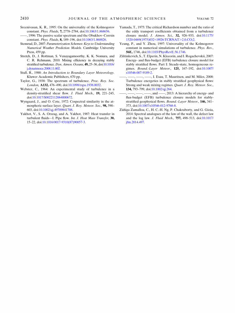
Sreenivasan, K. R., 1995: On the universality of the Kolmogorov

constant. Phys. Fluids, 7, 2778–2784, doi:10.1063/1.868656.

——, 1996: The passive scalar spectrum and the Obukhov–Corrsin

constant. Phys. Fluids, 8, 189–196, doi:10.1063/1.868826.Stensrud, D., 2007: Parameterization Schemes: Keys to Understanding

Numerical Weather Prediction Models. Cambridge University

Press, 459 pp.

Stretch, D., J. Rottman, S. Venayagamoorthy, K. K. Nomura, and

C. R. Rehmann, 2010: Mixing efficiency in decaying stably

stratified turbulence.Dyn. Atmos. Oceans, 49, 25–36, doi:10.1016/

j.dynatmoce.2008.11.002.

Stull, R., 1988: An Introduction to Boundary Layer Meteorology.

Kluwer Academic Publishers, 670 pp.

Taylor, G., 1938: The spectrum of turbulence. Proc. Roy. Soc.

London, A132, 476–490, doi:10.1098/rspa.1938.0032.Webster, C., 1964: An experimental study of turbulence in a

density-stratified shear flow. J. Fluid Mech., 19, 221–245,

doi:10.1017/S0022112064000672.

Wyngaard, J., and O. Cote, 1972: Cospectral similarity in the at-

mospheric surface layer. Quart. J. Roy. Meteor. Soc., 98, 590–

603, doi:10.1002/qj.49709841708.

Yakhot, V., S. A. Orszag, and A. Yakhot, 1987: Heat transfer in

turbulent fluids—I. Pipe flow. Int. J. Heat Mass Transfer, 30,15–22, doi:10.1016/0017-9310(87)90057-3.

Yamada, T., 1975: The critical Richardson number and the ratio of

the eddy transport coefficients obtained from a turbulence

closure model. J. Atmos. Sci., 32, 926–933, doi:10.1175/

1520-0469(1975)032,0926:TCRNAT.2.0.CO;2.

Yeung, P., and Y. Zhou, 1997: Universality of the Kolmogorov

constant in numerical simulations of turbulence. Phys. Rev.,

56E, 1746, doi:10.1103/PhysRevE.56.1746.

Zilitinkevich, S., T. Elperin, N.Kleeorin, and I. Rogachevskii, 2007:

Energy- and flux-budget (EFB) turbulence closure model for

stably stratified flows. Part I: Steady-state, homogeneous re-

gimes. Bound.-Layer Meteor., 125, 167–192, doi:10.1007/

s10546-007-9189-2.

——, ——, ——, ——, I. Esau, T. Mauritsen, and M. Miles, 2008:

Turbulence energetics in stably stratified geophysical flows:

Strong and weak mixing regimes. Quart. J. Roy. Meteor. Soc.,

134, 793–799, doi:10.1002/qj.264.

——, ——, ——, ——, and ——, 2013: A hierarchy of energy- and

flux-budget (EFB) turbulence closure models for stably-

stratified geophysical flows. Bound.-Layer Meteor., 146, 341–373, doi:10.1007/s10546-012-9768-8.

Zúñiga Zamalloa, C., H. C.-H. Ng, P. Chakraborty, and G. Gioia,

2014: Spectral analogues of the law of the wall, the defect law

and the log law. J. Fluid Mech., 757, 498–513, doi:10.1017/jfm.2014.497.

2410 JOURNAL OF THE ATMOSPHER IC SC IENCES VOLUME 72