Embed Size (px)
Citation preview

RISK MANAGEMENT AND DECISION THEORY
A promising marriage between two wholly
remarkable characters of mind-boggling lineage

Risk management and decision theory 1
Author: V. Versluis
Student number: 0809019
Email address: [email protected] / [email protected]
Group: BE44
Course: Bachelor Business Economics at Rotterdam University of
Applied Sciences
Principal initiator: A. F. de Wild
Email address: [email protected]
Organisation: Rotterdam University of Applied Sciences
Department: Enterprise Risk Management
Supervisor: H. J. J. de Breet
Email address: [email protected]
Second reader: S. Drigpal
Email address: [email protected]

Risk management and decision theory 2
Acknowledgements
It has been a rather educative blast, so to speak. I am proud to come to the zenith of my
venture into the world of risk management and decision theory with this dissertation.
Although this product is not my average type of product, as it is more theoretical and
mathematically challenging than most other projects I have finished during my course, I
found the process of concocting this dissertation a pleasure to the mind.
During the minor Enterprise Risk Management in the seventh semester, I took the
opportunity to make myself acquainted with the marvels of the ever captivating field of
decision theory through a series of lectures and a project. I am well pleased that I made
the decision for decision theory as the topic of my dissertation.
First of all, a very well meant thank you to Arie de Wild who gave me the opportunity to
write this dissertation and also helped me with my research. If it were not for this man
of great intellect, I would have never gotten interested in decision theory in the first
place. Also I would like to thank my supervisor for keeping me on track and, along with
the second reader, for assessing my aptitude in the field of Business Economics.
To my loving other half, a great thank you for giving feedback on the language
component of my dissertation and for putting up with my everlasting ramblings and
inquiries on how words are properly spelt. To my parents, thank you for giving me the
opportunity to study and always supporting me. Also to the rest of the people around
me, I extend my sincere gratitude.
Risk management and decision theory 3
Table of contents
Executive summary ....................................................................................................................................... 5
Introduction ..................................................................................................................................................... 7
1 Theory ....................................................................................................................................................... 9
1.1 Risk management ......................................................................................................................... 9
1.1.1 Risk management process .............................................................................................. 10
1.1.2 Risk matrix ........................................................................................................................... 11
1.1.3 Risk responses .................................................................................................................... 13
1.1.4 Making risk management decisions ........................................................................... 14
1.2 Decision theory............................................................................................................................ 15
1.2.1 Risk appetite and risk attitude ..................................................................................... 15
1.2.2 Expected value .................................................................................................................... 17
1.2.3 Expected utility ................................................................................................................... 17
1.2.4 Loss aversion ....................................................................................................................... 20
1.2.5 Prospect theory .................................................................................................................. 22
1.3 Risk management’s and decision theory’s common ground ..................................... 25
1.4 Decision influencing factors ................................................................................................... 25
1.4.1 Demographic and socioeconomic factors ................................................................. 26
1.4.2 DOSPERT ............................................................................................................................... 26
2 Experimental design .......................................................................................................................... 28
2.1 Desired information .................................................................................................................. 29
2.2 Risk reduction .............................................................................................................................. 30
2.2.1 Overview ............................................................................................................................... 30
2.2.2 Costs of control and axis values ................................................................................... 32
2.2.3 Manipulations...................................................................................................................... 33
2.3 Indifferences ................................................................................................................................. 35

Risk management and decision theory 4
2.4 Risk matrix .................................................................................................................................... 36
2.5 Demographic and socioeconomic factors ......................................................................... 36
2.6 DOSPERT ........................................................................................................................................ 36
3 Analysis .................................................................................................................................................. 37
4 Conclusion ............................................................................................................................................. 38
References ...................................................................................................................................................... 39
Appendix 1 – Example of a hypothetical participant ..................................................................... 41
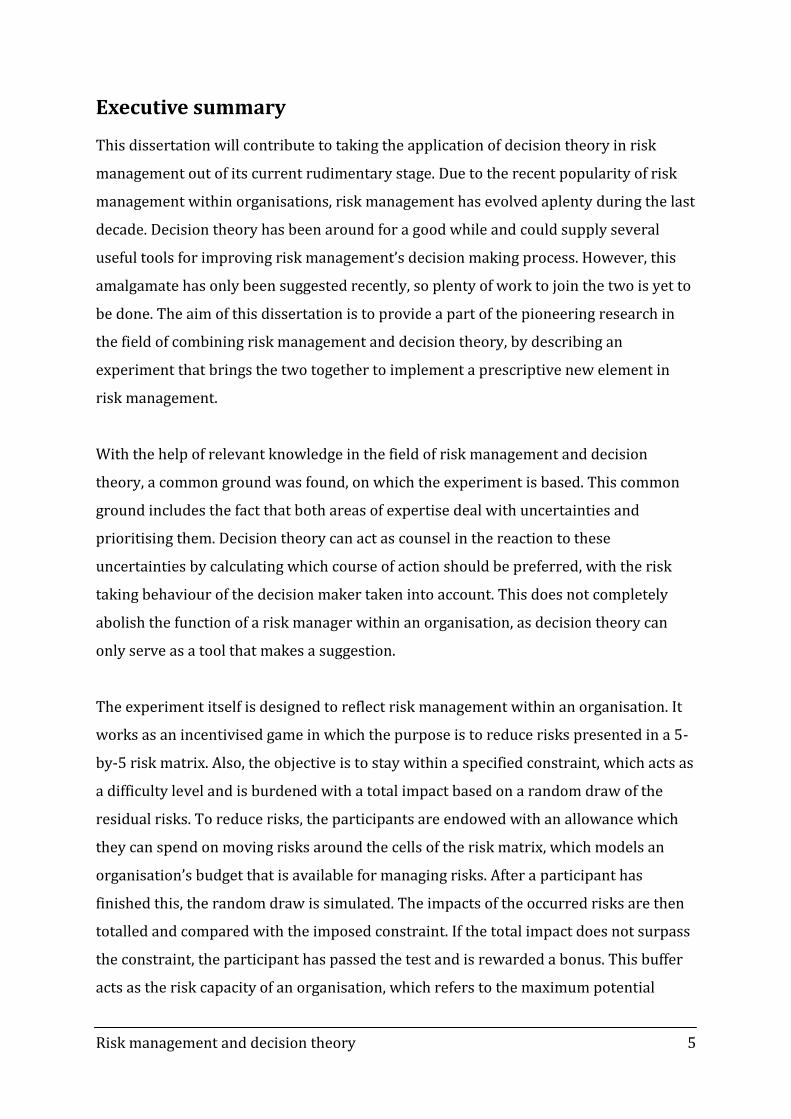
Risk management and decision theory 5
Executive summary
This dissertation will contribute to taking the application of decision theory in risk
management out of its current rudimentary stage. Due to the recent popularity of risk
management within organisations, risk management has evolved aplenty during the last
decade. Decision theory has been around for a good while and could supply several
useful tools for improving risk management’s decision making process. However, this
amalgamate has only been suggested recently, so plenty of work to join the two is yet to
be done. The aim of this dissertation is to provide a part of the pioneering research in
the field of combining risk management and decision theory, by describing an
experiment that brings the two together to implement a prescriptive new element in
risk management.
With the help of relevant knowledge in the field of risk management and decision
theory, a common ground was found, on which the experiment is based. This common
ground includes the fact that both areas of expertise deal with uncertainties and
prioritising them. Decision theory can act as counsel in the reaction to these
uncertainties by calculating which course of action should be preferred, with the risk
taking behaviour of the decision maker taken into account. This does not completely
abolish the function of a risk manager within an organisation, as decision theory can
only serve as a tool that makes a suggestion.
The experiment itself is designed to reflect risk management within an organisation. It
works as an incentivised game in which the purpose is to reduce risks presented in a 5-
by-5 risk matrix. Also, the objective is to stay within a specified constraint, which acts as
a difficulty level and is burdened with a total impact based on a random draw of the
residual risks. To reduce risks, the participants are endowed with an allowance which
they can spend on moving risks around the cells of the risk matrix, which models an
organisation’s budget that is available for managing risks. After a participant has
finished this, the random draw is simulated. The impacts of the occurred risks are then
totalled and compared with the imposed constraint. If the total impact does not surpass
the constraint, the participant has passed the test and is rewarded a bonus. This buffer
acts as the risk capacity of an organisation, which refers to the maximum potential
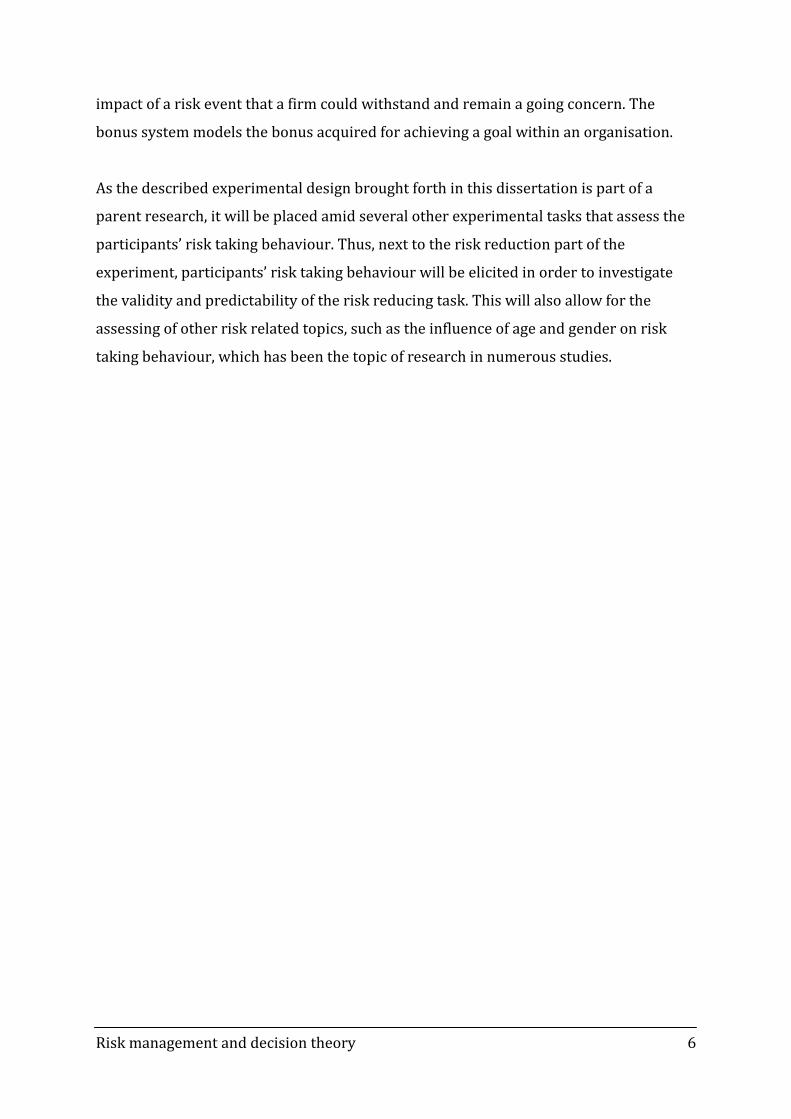
Risk management and decision theory 6
impact of a risk event that a firm could withstand and remain a going concern. The
bonus system models the bonus acquired for achieving a goal within an organisation.
As the described experimental design brought forth in this dissertation is part of a
parent research, it will be placed amid several other experimental tasks that assess the
participants’ risk taking behaviour. Thus, next to the risk reduction part of the
experiment, participants’ risk taking behaviour will be elicited in order to investigate
the validity and predictability of the risk reducing task. This will also allow for the
assessing of other risk related topics, such as the influence of age and gender on risk
taking behaviour, which has been the topic of research in numerous studies.

Risk management and decision theory 7
Introduction
With an ever progressing world comes risk in all fields imaginable. To triumph over all
of these risks would be tremendously hard, if not impossible. For several decades, risk
management has evolved into a discipline that is applied by many organisations to
overcome these ubiquitous risks.
Decision theory is concerned with calculating the consequences of uncertain decisions.
This science has been present ever since Pascal came up with the idea of calculating
expected value for uncertain decisions in the 17th century. Ever since, decision theory
has evolved and is now used to describe decision making processes in various fields,
such as economics, mathematics and psychology, on a higher level than just Pascal’s
calculation of expected value.
As risk management is concerned with making decisions to manage uncertainties and
their consequences and decision theory is concerned with evaluating choices people
make, it would seem that these two disciplines share a common ground and are often
used jointly. However, the only part of decision theory that is usually applied to risk
management is calculating the expected value of a risk, whilst other aspects of decision
theory are seldom used. This dissertation will contribute to the ongoing evolution of
risk management by bringing risk management and decision theory together more
closely and take the current application of decision theory in risk management out of its
current rudimentary stage.
This dissertation is written within the confines of a parent research, which strives to
“contribute to tightening the gap between the practice and promise of decision theory in
the field of risk management” (De Wild, forthcoming). The research described in this
dissertation is focussed on part of an experiment to gauge organisational risk appetite.
A clear definition of an organisation’s risk appetite can be used as a guideline in the
decision making process regarding risks. In the experimental part described in this
dissertation, participants will be subjected to risks within a risk matrix and is given the
opportunity to invest in reduction measures. The residual risks can subsequently be
analysed and the participants’ risk appetite can be assessed.

Risk management and decision theory 8
The problem at hand is defined as “creating an experiment that allows for the
assessment of risk appetite within a risk reduction context through application of the
risk matrix”. The main research question is thus:
“How can risk appetite in the context of risk reduction be experimentally assessed
through application of a risk matrix?”
To answer this question, several other questions can be posed, to come to the answer of
the main research question:
What is the common ground of risk management and decision theory?
How can decision theory be used together with a risk matrix?
How can risk appetite be derived from a reduced risk matrix?
The parent research will provide a new perspective on risk appetite within
organisations, which can assist risk management practitioners in determining the
acceptable level of risk within an organisation and can thus further integrate decision
theory in risk management. As merge has been suggested only recently, research can
form the foundation of a valuable new eye-opening facet of risk management that
provides insight in the risk taking behaviour of organisations. This dissertation provides
part of the research necessary to achieve the intention of the parent research, by
providing the basis for approaching risk appetite through application of a risk matrix.
In the first chapter a range of relevant theory regarding risk management and decision
theory will be evaluated and common grounds shared by the two disciplines will be
uncovered. In the second chapter the experimental method used to assess risk appetite
through application of the risk matrix will be discussed. It will also swiftly go over other
parts of the experiment employed in the parent research. In the third chapter a
conclusion will be drawn to answer the questions posed in this introduction. In chapter
four several recommendations will be made on how the results of the experiment
designed in chapter three can be used for further research.

Risk management and decision theory 9
1 Theory
To create an experiment that uncovers risk appetite, it is necessary to first construct an
appropriate theoretical framework to place it in. This chapter will first discuss risk
management as it is applied in organisations, showing its goals, application and a
popular risk management tool called the risk matrix. Paragraph two will discuss
decision theory and how it can be applied to risk management. The presented theory in
the first two paragraphs will only include theory that is relevant to this dissertation. The
third paragraph will reflect on the previous two paragraphs and bring forth the
common ground of risk management and decision theory. In the last paragraph passive
traits influencing risk taking will be discussed.
1.1 Risk management
Risk is the possibility that an event will occur and adversely affect the achievement of
objectives. Risk management is the process that attempts to manage the uncertainty
that influences the achievement of objectives, with the goal of reaching the objectives
and thus creating value for the organisation in which it is applied (COSO, 2004). In order
to accomplish this goal, it is necessary to constantly apply risk management throughout
all of the aspects of an entity.
Risk management attempts to identify risks and take appropriate action to diminish
their impending effects on an organisation. As the process of risk management is rather
abstract, several risk management standards, such as COSO, FERMA and CAS, have been
developed. The guidelines offered by these standards are broadly applicable and make
it possible to approach risks in a great variety of contexts, from financial portfolio risk
to health care and from oil drilling to organising sports events.
Risk management and decision theory 10
1.1.1 Risk management process
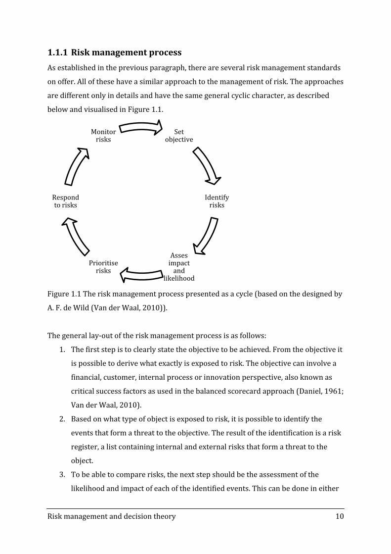
As established in the previous paragraph, there are several risk management standards
on offer. All of these have a similar approach to the management of risk. The approaches
are different only in details and have the same general cyclic character, as described
below and visualised in Figure 1.1.
Figure 1.1 The risk management process presented as a cycle (based on the designed by
A. F. de Wild (Van der Waal, 2010)).
The general lay-out of the risk management process is as follows:
1. The first step is to clearly state the objective to be achieved. From the objective it
is possible to derive what exactly is exposed to risk. The objective can involve a
financial, customer, internal process or innovation perspective, also known as
critical success factors as used in the balanced scorecard approach (Daniel, 1961;
Van der Waal, 2010).
2. Based on what type of object is exposed to risk, it is possible to identify the
events that form a threat to the objective. The result of the identification is a risk
register, a list containing internal and external risks that form a threat to the
object.
3. To be able to compare risks, the next step should be the assessment of the
likelihood and impact of each of the identified events. This can be done in either
Set objective
Identify risks
Asses impact
and likelihood
Prioritise risks
Respond to risks
Monitor risks

Risk management and decision theory 11
or both a qualitative or quantitative way. Assessment of impact is done in
relevant quantities, in most cases this is done in monetary equivalents, but it is
common to see impact expressed in other quantities, such as reputational
damage and injuries.
4. Prioritisation of risks is done by comparing individual risks. This can be done in
several ways. Frequently used methods of prioritisation are the expected value
method, which ranks risks according to the product of a risk’s probability and
impact, and plotting risks on a risk matrix, which offers a visual aid to compare
risks. A more detailed description of risk matrices is supplied in paragraph 1.1.2.
5. When risks have gone through the prioritising step, an appropriate risk response
is applied to deal with the risk. Possible risk responses include treat, transfer,
terminate and tolerate. These responses to risk will be described in more detail
in paragraph 1.1.3.
6. After selecting an appropriate risk response, the risk should be monitored to
ensure it will not become a threat again. Depending on the severity of the
residual risk, reassessment can be done on daily to an annual basis. This final
step in the risk management process serves as a monitoring and feedback
moment and closes the cycle of risk management.
1.1.2 Risk matrix
Risk matrices are widely used as a tool to visualise various types of risk. The use of risk
matrices is promoted by several risk management standards (FERMA, 2002; COSO,
2004). A risk matrix is a rendering of a probability and a consequence axis in the form of
a graph. The axes are divided in several categories, ranging from low to high. The
resolution of this matrix depends on the amount of categories along the axes and is an
arbitrary choice by the creator of the matrix. It is possible to give the axes both
qualitative and quantitative labels. As a result the categories might not be linear in the
case of quantitative labels. For quantitative labels a percentage is used for the
probability axis and the consequence axis is usually expressed in monetary terms.
Depending on the type of risks plotted in the risk matrix, another scale can be used,
such as injuries or reputational damage. The two axes create a number of cells, each
representing a range of probability and a range of consequence. To enhance the
visibility of the risk matrix, colours or numbers are commonly used to indicate the

Risk management and decision theory 12
acceptability of each of the cells. Colours and numbers ranging from green or 1
(acceptable) to red or 5 (unacceptable) are most often used for this and can be
arbitrarily applied to every cell. An example of a risk matrix is shown in Figure 1.2.
Figure 1.2 An example of a 5-by-5 qualitative risk matrix, with a numerical and colour
scale indicating the acceptability of every cell, ranging from acceptable (1 and green) to
unacceptable (5 and red).
Note that the risk matrix is not necessarily symmetric with respect to the diagonal. This
can be explained by the fact that the range of every category can be arbitrarily chosen
and that the last category of the consequence axis is where risks such as bankruptcy,
death or irreparable damage are located. As these risks have an irrecoverable impact,
they can practically never be grouped with any acceptable risks.
When identified risks are plotted in the risk matrix, they can be ranked for urgency as a
result of prioritisation by the colour of the cell in which they are located. The
acceptability index can also be used to roughly outline which control measures should
be taken to manage risks (Glasgow Caledonian University, 2009). A red cell means that a
risk is unacceptable and should be treated, transferred or terminated immediately. A
risk located in an amber cell is momentarily acceptable, but should be considered for
treatment or transferring shortly. Depending on the severity of the consequence, a risk
located in an amber area could also be tolerated. Risks in a green cell can be tolerated or
treated, depending on impact and probability.
Very likely 2 3 4 4 5
Likely 2 3 3 4 5 1 Acceptable
Possible 2 2 3 4 4
Unlikely 1 2 3 3 4 5 Unacceptable
Very unlikely 1 1 2 3 3
Very sm
all
Small
Mo
derate
Large
Very large
Lik
elih
oo
d
Impact
Risk management and decision theory 13
Although the use of risk matrices is commonplace, the simple application of it comes
with several disadvantages (Cox, 2008):
- Risk matrices are prone to poor resolution, as there can usually only be a rough
indication of probability and consequence of risks;
- Due to the range used per category, a risk can be assigned a wholly erroneous
level of probability or consequence;
- Risk reactions cannot be based on solely the probability and consequence
categories and;
- Qualitative categorisation leads to subjective rating of risks.
Avoiding these limitations of risk matrices can be done by assigning a definite value to
each category of the risk matrix whilst expressing risks in an objective quantitative
measure, to prevent ambiguous interpretation of risks. Still, even a quantitative
approach leaves room for errors due to the necessity of subjectively assigned likelihood
and impact to risks unfamiliar to an organisation.
1.1.3 Risk responses
After assessing relevant risks, a proper response to each of the risks must be
implemented. Possible responses are termination (avoidance), treatment (reduction),
transfer (sharing) and toleration (acceptance) (COSO, 2004). In the list below, the risk
responses are explained into further detail. First the response is named, followed by the
COSO definition and an example:
- Terminate, completely shutting off all activities that cause the risk to exist. This
happens when for example manufacturing a certain product is not viable for
profit anymore. In this case a company can choose to stop manufacturing the
product.
- Treat, reducing either or both the impact or probability of the risk directly. For
example, the risk of fire can be treated by reducing either the impact or
probability separately. To reduce the impact of the fire, a curative measure is
taken, usually with no effect on the risk’s probability. This could be done by
installing a sprinkler installation. On the other hand, a preventive measure can
be taken to reduce the likelihood of a fire occurring. This is usually done by the
use of materials impregnated with fire retardant agents, to avoid material from
Risk management and decision theory 14
bursting into flames. The preventive measure, in turn, does not always affect the
risk’s impact directly.
- Transfer, fully or partially reducing the impact or probability of the risk by a full
transfer or sharing of a risk. The obvious example of this response is an
insurance policy. When an organisation or person is not able to cover the impact
of a risk, an insurer can be approached to cover the risk for a certain payment.
- Tolerate, leaving the risk as is without taking any action. This can be done when
a risk is of negligible size and is considered an acceptable risk, either before or
after the implementation of other risk responses, and cannot be further
responded to. Otherwise, a risk of substantial size can be tolerated if the
presence of the risk is vital for the existence and continuity of an organisation.
Any risks that remain and are tolerated should be subjected to monitoring, for
they should not evolve from a tolerated acceptable risk into an unacceptable risk.
An organisation can choose which response or combination thereof should be employed
to counter a specific risk. To determine the best fitting response for a risk, the
organisation should consider risk tolerance and the effects of the available responses on
the organisation on a broad level. Also opportunities arising from both the bare risk as
the response and a cost-benefit analysis should be taken into account.
1.1.4 Making risk management decisions
In the cycle of risk management, the step that creates value for an organisation is chiefly
selecting the appropriate risk responses to counter risk. For financial risks this choice is
often a case of optimisation, as the goal is to find a balance between the cost of the
reaction to be applied and the residual risk after application. It is important to note that
the decision maker’s attitude towards the impending risk has influence on the process
of choosing the suitable reaction to deal with the risk. This leads to a person more
lenient towards taking risk to sooner find a risk tolerable than a person more hesitant
towards taking risk. Likewise, depending on the decision maker, a risk might be
completely terminated, whereas someone else would find reduction preferable. To
describe risk preferences, decision theory can be applied for a more mathematical
approach to choices involving risks.

Risk management and decision theory 15
1.2 Decision theory
Decision theory is the part of probability theory that is concerned with calculating the
consequences of uncertain decisions. This can be applied to state the objectivity of a
choice and to optimise decisions. In this paragraph several aspects of decision theory
will be discussed, being risk appetite, risk attitude, expected value, expected utility, loss
aversion and prospect theory.
1.2.1 Risk appetite and risk attitude
A clear description of risk appetite allows for a consistent approach to handling risks
within an organisation. The definition of risk appetite is the amount of risk, on a broad
level, an entity is willing to accept in pursuit of value (COSO, 2004). Another term that is
associated with this is risk attitude, which describes the tendency to risk averse, risk
seeking or risk neutral behaviour. In other words, risk appetite relates to taking risks in
a broad sense and risk attitude relates to making a risky decision. Risk attitude can be
elicited from the upper echelon of an organisation and thus expressed in a quantitative
manner by use of risk appetite, which reflects risk taking behaviour. This information
can be formally published in a document such as a risk policy, which is an asset to an
organisation by means of making it possible to handle risks in a reliable way.
An agent’s risk attitude can be elicited in a relatively straightforward way. When an
agent is offered a choice between a risky and a safe option, the agent chooses and their
preference is found. Depending on the choice the agent made, the sure option is made
more or less attractive, after which the agent makes their choice again. This process can
be repeated several times to iterate towards a point where both options are equally
attractive and thus a point of indifference is reached. Such methods of eliciting risk
attitude have been successfully used in experiments (Keeney & Raiffa, 1976; Pennings &
Smidts, 2000). Example 1 illustrates this method. This example forms a crux for
explaining several necessary concepts to calculate risk appetite throughout this
dissertation.
Risk management and decision theory 16
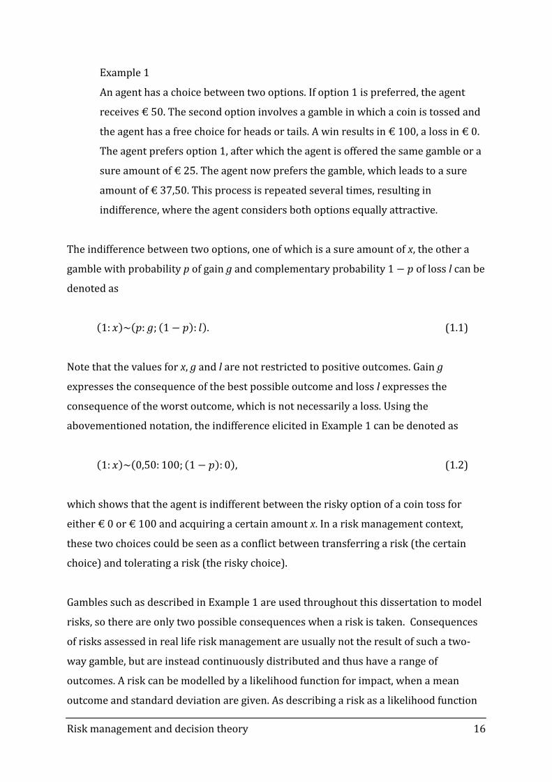
Example 1
An agent has a choice between two options. If option 1 is preferred, the agent
receives € 50. The second option involves a gamble in which a coin is tossed and
the agent has a free choice for heads or tails. A win results in € 100, a loss in € 0.
The agent prefers option 1, after which the agent is offered the same gamble or a
sure amount of € 25. The agent now prefers the gamble, which leads to a sure
amount of € 37,50. This process is repeated several times, resulting in
indifference, where the agent considers both options equally attractive.
The indifference between two options, one of which is a sure amount of x, the other a
gamble with probability p of gain g and complementary probability of loss l can be
denoted as
. (1.1)
Note that the values for x, g and l are not restricted to positive outcomes. Gain g
expresses the consequence of the best possible outcome and loss l expresses the
consequence of the worst outcome, which is not necessarily a loss. Using the
abovementioned notation, the indifference elicited in Example 1 can be denoted as
, (1.2)
which shows that the agent is indifferent between the risky option of a coin toss for
either € 0 or € 100 and acquiring a certain amount x. In a risk management context,
these two choices could be seen as a conflict between transferring a risk (the certain
choice) and tolerating a risk (the risky choice).
Gambles such as described in Example 1 are used throughout this dissertation to model
risks, so there are only two possible consequences when a risk is taken. Consequences
of risks assessed in real life risk management are usually not the result of such a two-
way gamble, but are instead continuously distributed and thus have a range of
outcomes. A risk can be modelled by a likelihood function for impact, when a mean
outcome and standard deviation are given. As describing a risk as a likelihood function

Risk management and decision theory 17
of a consequence during an experiment would most likely not go down well with
participants, not to mention the person analysing the results, risks are modelled as a
two way gamble in decision theory.
To assess the agent’s risk attitude with regards to the method employed in Example 1,
the expected value of the two choices needs to be calculated. This is a fairly simple
approach and will be described in the following paragraph.
1.2.2 Expected value
The two options in indifference (1.1) are equally attractive to the agent. However,
calculating the expected value of the two choices, using the well known general
definition of expected value,
, (1.3)
where expected value EV is the sum of all products of an option with n possible
outcomes with possibility p and consequence x for every possible outcome, it can be
shown that the certain and uncertain choice should not be equally attractive, as an
objective decision maker should be indifferent when the expected value of both options
are identical. From this, the expected value can be used to assess the risk attitude of the
agent. If EVc is the expected value of the certain option to obtain amount x and EVr is the
expected value of the risky option that involves a gamble, then for the agent
is risk seeking, for the agent is risk averse and for the agent is risk
neutral. By using the expected value to gauge an agent’s indifference between the two
options, it is not possible to explain why an indifference is obtained where .
For an objective agent, this would not be true. To explain this phenomenon, another
approach to indifferences is employed, namely expected utility.
1.2.3 Expected utility
In the world of economics, utility is used as a measurement of satisfaction. This can also
be used in decision theory, as a means of expressing the satisfaction of a particular
choice, as illustrated in Example 1. When indifference is reached, the satisfaction that
the options carry is the same. To allow for easy comparison between different positive

Risk management and decision theory 18
amounts of money, a scale of 0 to 1 is used, where the highest possible amount of money
xmax in a given frame is denoted as . A zero amount of money constitutes to
no change in utility, thus . For values of x between 0 and xmax, the utility is
expressed as a value relative to xmax. This can also be applied to situations with
exclusively negative outcomes and both positive and negative outcomes, which leads to
negative utility. It is also possible to extend this framework to include possibilities of
outcomes, which leads to the expected utility of an outcome.
The expected utility of an outcome, with consequence x and probability p, is calculated
by multiplying the probability and the utility of the consequence, so that
. (1.4)
This definition of expected utility can be used to evaluate indifferences between a
certain and a risky option. Taking indifference (1.1), by assuming the certain option is of
the same expected utility as the two possible outcomes of the uncertain option, this
results in
. (1.5)
If this is applied to Example 1, it can be shown that for indifference between a risky
option with equally probable outcomes of € 0 or € 100 and a certain option involving an
amount of money x, then
. (1.6)
This property of the gamble used in the example allows for simple plotting of
indifference curves, using the outcome of the indifference. This is shown Figure 1.3
below.

Risk management and decision theory 19
Figure 1.3 The utility of gain x for three agents with different risk attitudes.
Figure 1.3 shows the utility curve of three agents with different indifferences elicited
using the method in Example 1. This illustrates the law of diminishing marginal utility
for risk aversion, which implies that the first units gained, in this case the first few
Euros, yield more pleasure than the last units gained (Wicksteed, 1910). In contrast, risk
seeking behaviour implies the opposite. Risk neutrality implies a linear utility, where
every Euro is valued equally.
In order to create the curve using a mathematical approach, a frequently used equation
is the exponential equation
, (1.7)
where utility is a function of amount of money x and risk tolerance R. Risk tolerance is
the range of acceptable variation an entity is willing to accept to achieve an objective
(COSO, 2004) and is expressed as an amount of x, so that it represents the variation
within a reference frame of x. This implies that risk tolerance R should be in the same
order of magnitude as amount x. Applying equation (1.7) to find the utility of a specific x
may not yield a result that fits in the aforementioned frame of utility for positive
0,00
0,25
0,50
0,75
1,00
0 25 50 75 100
Uti
lity
U(x
)
Amount x in Euros
Utility of gain x
Risk averse (x = € 25)
Risk neutral (x = € 50)
Risk seeking (x = € 75)

Risk management and decision theory 20
consequences of x, . To allow for easy comparison between utilities within
a particular frame, the acquired utility U(x) using equation (1.7) is divided by the utility
of the highest possible consequence within the frame, U(xmax). This approach is valid for
possible gains, as well as possible losses.
In the utility approach to risk aversion, applying equation (1.7), it implies that risk
aversion is present for , risk seeking behaviour for and risk neutrality for
. Overall, people are inclined to establish a sure amount of wealth in gain
scenarios, leading to risk aversion in the gains domain. Conversely, people tend to take a
gamble to nullify a certain loss, leading to risk seeking behaviour in the losses domain
(Kahneman & Tversky, 1979). Combining a gain and loss scenario within the same
gamble is further explored in paragraph 1.2.4.
1.2.4 Loss aversion
As established in paragraph 1.2.3, people in general would rather take a decent sized
certain gain than gamble for a potential large gain and in contrast are willing to take a
gamble to avoid a certain loss. This leads to the aphorism “losses loom larger than
gains”, meaning that in the sense of utility, for most people the pleasure derived from
obtaining some specific amount of money is less than the displeasure that is felt when
that specific amount is lost. This has been experimentally confirmed (Kahneman &
Tversky, 1979) and can be seen in the graph in Figure 1.4.

Risk management and decision theory 21
Figure 1.4 The value function graphically demonstrating loss aversion, expressed in
bacon. The loss of a specific amount of bacon looms larger than the gain of the same
amount of bacon.
Figure 1.4 presents the value function, which shows the characteristic curves in both
the gains and losses domains, indicating risk averse behaviour for gains and risk
seeking behaviour for gains. Additionally, the steeper inclination of the function in the
losses domain illustrates how a loss looms larger than a gain. The apparent difficulty of
a loss can be caused by the status quo bias (Samuelson & Zeckhauser, 1988; Novemsky
& Kahneman, 2005) which indicates that most do not like giving up a good and require a
sizeable compensation in order to give up a good.
In an experimental approach, loss aversion can be measured by giving a decision maker
two options. The first option is the status quo choice, a certain option with no
consequence, so that there is a 100% chance of acquiring € 0. The second choice is a
mixed prospect, with a possible downside and upside consequence. By adjusting the
second option, making it more or less attractive depending on the preferred choice, the
agent iterates towards indifference, similar to the approach in Example 1. This leads to
an indifference rather like indifference (1.1), but with , aling the agent to choose
for a status quo option. This yields indifference
, (1.8)

Risk management and decision theory 22
where a balance exists between the status quo and a mixed prospect, with probability p
of incurring a gain g and a complementary probability of incurring loss l. If the agent
acts according to the expected value theorem, in case of equal probabilities of the
positive and negative consequence occurring, then . However, if the agent shows
signs of loss aversion, then , as the possible gain must overcompensate the
possible loss.
The sunk cost effect can be explained with loss aversion (Knox & Inkster, 1968). Sunk
costs are costs sustained in the past that cannot be recovered and thus are seen as a
loss. What follows from this is the sunk cost fallacy, which describes that after a hefty
investment in an on-going project that led to only a poor return, investments are kept
being made in the hopes of a gain compensating for the loss, even though the best
option on paper would be to pull out of the project. This is also colloquially called the
Concorde fallacy, which refers to how the Concorde project should have been cancelled
based on financial returns, whilst the British and French governments kept investing in
the hope to turn the project into a profitable business.
Loss aversion is closely related to the endowment effect (Kahneman, Knetsch, & Thaler,
1990), which describes that people value an endowed good more than they would a
good that is not endowed. Typically, to sell an endowed good, people demand more than
they would sacrifice for the same good, if they were to purchase it. Studies have varying
success producing loss aversion, indicating that a significant difference exists
(Kahneman, Knetsch, & Thaler, 1990; Tversky & Kahneman, 1991) to little to no
evidence of loss aversion or the endowment effect going on at all (Harinck, Van Dijk, Van
Beest, & Mersmann, 2007; Ert & Erev, 2008). Also, the buying and selling price does not
depend on actual physical endowment of the bought or sold item in question (Carmon &
Ariely, 2000), which means loss aversion also occurs when a hypothetical prospect is at
stake, which is good news for experiments dealing with loss aversion.
1.2.5 Prospect theory
In paragraph 1.2.3 it has been shown that the utility function for money is nonlinear and
has a slight concave curve for people in general, which implies diminishing marginal
utility. This phenomenon indicates that if an amount of money is expressed as its utility

Risk management and decision theory 23
equivalent, half the amount of money is not necessarily assigned half the utility
equivalent of the double amount, so is not necessarily valid. To fall back
on a risk context, this means that the consequence is interpreted subjectively and
consequences of independent risks cannot be compared linearly. Peculiarly enough, this
difficulty in comparing is not restricted to the monetary property of a risk, but is also
present in the probability property of a risk, so if p is some probability and w(p) is its
perceived probability then is not necessarily valid. Prospect theory explains
this phenomenon and applies it to gambles.
Well-defined numerical probabilities should provide an agent with information to make
an objective decision. However, the numerically expressed probabilities are interpreted
subjectively and as a result the agent either exaggerates or undervalues said probability.
Typically low probabilities are seen as higher than they really are, whilst high
probabilities are seen as lower (Kahneman & Tversky, 1979). A graph illustrating this
typical probability weighting is shown in Figure 1.5, where p is an objectively expressed
probability and w(p) is the subjective probability an agent assigns to p.
Figure 1.5 An example of a typical probability weighting curve with overweighting for
small probabilities and underweighting for high probabilities.
0
0,2
0,4
0,6
0,8
1
0 0,2 0,4 0,6 0,8 1
We
igh
ted
pro
bab
ility
w(p
)
Probability p
Probability weighting of probability p
w(p)
p = w(p)

Risk management and decision theory 24
The probability weighting function as shown in Figure 1.5 applies to both gains and
losses, which leads to optimism for potential gains with low probability and pessimism
for gains with high probability. In the same way this leads to pessimism for losses with
low probability and optimism for losses with high probability. Using this understanding
of probability, it can be explained how a jackpot is an exciting prospect for a lottery
ticket owner, even though it is very unlikely they will win the jackpot. This can also
explain risks with consequences that are not expressed in monetary terms, such as
bungee jumping and cricket. These activities are safe to enjoy, but involve risks with a
fatal impact, but very low probability, yet these sports are not practiced as a pastime on
a daily basis by many people, as they are considered dangerous.
Identical to expected utility, prospect theory is used to assign a preference value to
gambles in order to rank the attractiveness of the complete prospect and not just the
monetary outcome. To do this, the weighted probability is simply multiplied by the
utility of the outcome, so that
, (1.9)
where PT(p,x) is the expected utility of a prospect with a weighted probability w(p) of
probability p and utility U(x) of impact x.
Probability weighting functions as a correction for the probability in the same way as
utility functions as a correction for the impact of a risk. The elicitation of the probability
weighting function is done in a similar way (Abdellaoui, 2000) as the elicitation of the
utility function, as shown in paragraph 1.2.3. The probability weighting function itself
can be described with equation
, (1.10)
where α influences the area of p near 100% and β influences the area of p near 0%
(Lattimore, Baker, & Witte, 1992; Ostaszewski, Green, & Myerson, 1998; Wakker, 2008).
In the case of and , the function is linear, so that . Probability
Risk management and decision theory 25
weights assigned to probabilities for positive and negative outcomes do not necessarily
have to be identical and are called respectively w+ and w-.
1.3 Risk management’s and decision theory’s common ground
In paragraph 1.1 and 1.2, the cases of risk management and decision theory have been
partially discussed. The knowledge of these areas of expertise now allows for an
intersection of the two to find their common ground.
The most striking resemblance is that both risk management and decision theory would
not exist without the presence of uncertainties. Moreover, there are several similarities
when the risk management process is studied further. Risk management attempts to
assess uncertainties and prioritise them, which decision theory is able to do for the
latter. Risk management makes decisions to manage the uncertainties, whilst decision
theory can prescribe what the correct course of action would be to deal with the
uncertainty, if information on the risk taking behaviour of the decision maker is present.
Decision theory can be applied to prioritise risks in a similar fashion to the risk matrix.
When sufficient information on the decision maker’s risk taking behaviour is available,
the decision maker’s quantitative risk matrix can be predicted by calculating the utility
of the cells in the risk matrix, each of which indicates a range of risks. The result can be
used as an indication of priority, with risks in cells of the largest absolute utility having
higher priority than risks with lower absolute utility.
1.4 Decision influencing factors
The decisions people make can be assessed by using the methods described in
paragraph 1.2. These decisions are influenced by the personality and characteristics of
the decision maker. This paragraph will discuss which traits influence risk taking
behaviour and how risk taking behaviour expressed in nonfinancial areas can be used to
assess risk taking behaviour in financial areas.
Risk management and decision theory 26
1.4.1 Demographic and socioeconomic factors
Influence on risk taking behaviour of demographic and socioeconomic factors such as
age, sex and income status has been the subject in a number of researches. Research to
these factors is mostly done by means of a questionnaire, although doubts have been
raised over the reliability of this method. Questionnaires are said to do a poor job
predicting actual investment behaviour (Bouchey, 2004) and to have only little
correlation with reality (Yook & Everett, 2003). This creates an opportunity for a
different approach to verify or falsify the outcomes of earlier research.
The consensus in efforts to research demographic and socioeconomic factors
influencing risk taking decisions, appears to be that there is a positive correlation
between being more risk seeking and the following (Bajtelsmit & Bernasek, 1996; Sung
& Hanna, 1996; Grable, 2000):
- Being male;
- Being older;
- Being white;
- Being married;
- Being professionally employed with higher income;
- Having more education;
- Having more financial knowledge and;
- Having higher economic expectations.
1.4.2 DOSPERT
It is axiomatic that if one is prone to risky behaviour in one area, such as gambling, one
is likely to show risky behaviour in other areas as well, such as sports and health.
DOSPERT (Domain-Specific Risk-Taking) offers a psychometric scale that assesses risk
perception in five content domains, including financial, health and safety, recreational,
ethical and social decisions (Weber, Blais, & Betz, 2002; Blais & Weber, 2006). A person
is to indicate the likelihood of engaging in a number of activities in one or any of the
aforementioned domains, on a seven point scale, ranging from extremely unlikely to
extremely likely. The points assigned to an activity are directly translated into a score
and the sum of scores for all activities acts as an indication for the risk taking behaviour
of said person.

Risk management and decision theory 27
The financial DOSPERT domain contains a risk taking sub domain, this element can be
applied to research regarding risk taking behaviour. This domain contains opportunities
with a risky financial context:
- Investing 10% of your annual income in a moderate growth mutual fund;
- Betting a day’s income at the horse races and;
- Investing 5% of your annual income in a very speculative stock.

Risk management and decision theory 28
2 Experimental design
The goal of the experiment is to test the theoretical framework, as described in chapter
1. This is done by comparing the data gathered from three tasks, covering a model of a
risk reduction task in practice, an elicitation of indifferences as described in paragraph
1.2.1 and an assessment of a risk matrix. To test the underlying determining factors
influencing the participants’ risk appetite, several manipulations will find place during
the experiment.
The risk reduction task will show which risks are the most unacceptable ones in a
practical scenario. To ensure a reaction that reflects a real situation, the reduction task
involves real money and the goal for the participants is to maximise their earnings. In
this task, several manipulations will be implemented, so the risk reduction can
represent a number of different scenarios, all of which can be compared with one
another. The reduction task as well as the manipulations will be described in the second
paragraph.
In the second task the participants need to complete, risk attitude towards gains, losses
and mixed gambles will be obtained. The results of this task will be used to calculate the
participants’ risk aversion, probability weighting function and loss aversion, for gains as
well as losses. The second task is described in paragraph three.
The third part of the experiment is the rating of acceptability of each of the risks
involved in the first part of the experiment, which will be described in the fourth
paragraph. The result is a risk matrix. In conjunction with data on risk taking behaviour,
predictability of the risk matrix can be assessed.
In the final part of the experiment, the participants provide personal demographic,
socioeconomic and DOSPERT information for further study. This is described in
paragraph five and six.

Risk management and decision theory 29
2.1 Desired information
Following from the relevant theory in chapter 1, the actual experiment will consist of
several separate parts, each investigating another aspect of decisions under risk. To
achieve this, the experiment is divided in four distinct parts, being:
- Reduction of risks (paragraph 2.2);
- Finding indifferences(paragraph 2.3);
- Assessing a risk matrix (paragraph 2.4)and;
- Supplying relevant personal details(paragraph 2.5 and 2.6).
The reduction of risks will require participants to reduce a multitude of risks shown in
the cells of a risk matrix. To do this, the participants are endowed with a finite amount
of credits that can be spent on reducing risks along the probability or impact axis of the
matrix, by moving risks from cell to cell. The participants are free to decide which risks
should be reduced and which risks are left alone.
For the indifference part of the experiment the goal is to choose between two options to
reveal the risk preference of each of the participants. Depending on the choice of the
individual participants, one of the options will be made more or less attractive. By
repeating this, the participant will iterate towards a point where the participant is
considered indifferent between the options.
By assessing a risk matrix, participants’ personal risk matrices will be revealed. This is
done by making the participants indicate to what degree a cell within the risk matrix is
acceptable.
The final part of the experiment will provide demographic, socioeconomic and
DOSPERT data by the participants.

Risk management and decision theory 30
2.2 Risk reductionction
The first part of the experiment consists of reducing a number of risks plotted in a risk
matrix. In this paragraph the general overview of the risk reduction part of the
experiment will be given, as well as the cost of reducing single risks in this matrix. The
desired manipulations and their implementation will also be clarified.
2.2.1 Overview
For the first task, the participants are expected to reduce a number of risks, expressed
as a probability p of negative consequence x, without further context. In total 25 risks
will be presented to the participants, as defined by a 5-by-5 risk matrix, with 5
categories for both probability and consequence. This should give the outcome a
reasonable resolution, whilst keeping the experiment understandable to the
participants. Each cell in this matrix contains a unique risk that can be reduced by the
participants. A risk R(p,x) is defined as an event with probability p and consequence x,
illustrated in Figure 2.1.
Figure 2.1 A risk matrix with risk R(5,5). The values of p and x refer to the respective
categories the risk is located in.
When a participant is presented an unacceptable risk R(p,x), the participant can pay a
certain amount for control measures to reduce the risk in either or both the probability
or consequence domain. The remainder of the risk after application of the control
measures is now residual risk R’(p’,x’), as illustrated in Figure 2.2.
5 R
4
3
2
1
1 2 3 4 5
Pro
bab
ility
cat
ego
ry p
Impact category x
Risk management and decision theory 31
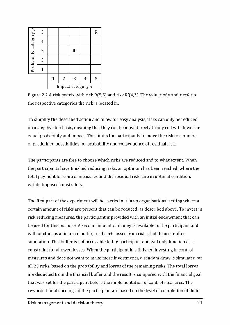
Figure 2.2 A risk matrix with risk R(5,5) and risk R’(4,3). The values of p and x refer to
the respective categories the risk is located in.
To simplify the described action and allow for easy analysis, risks can only be reduced
on a step by step basis, meaning that they can be moved freely to any cell with lower or
equal probability and impact. This limits the participants to move the risk to a number
of predefined possibilities for probability and consequence of residual risk.
The participants are free to choose which risks are reduced and to what extent. When
the participants have finished reducing risks, an optimum has been reached, where the
total payment for control measures and the residual risks are in optimal condition,
within imposed constraints.
The first part of the experiment will be carried out in an organisational setting where a
certain amount of risks are present that can be reduced, as described above. To invest in
risk reducing measures, the participant is provided with an initial endowment that can
be used for this purpose. A second amount of money is available to the participant and
will function as a financial buffer, to absorb losses from risks that do occur after
simulation. This buffer is not accessible to the participant and will only function as a
constraint for allowed losses. When the participant has finished investing in control
measures and does not want to make more investments, a random draw is simulated for
all 25 risks, based on the probability and losses of the remaining risks. The total losses
are deducted from the financial buffer and the result is compared with the financial goal
that was set for the participant before the implementation of control measures. The
rewarded total earnings of the participant are based on the level of completion of their
5 R
4
3 R'
2
1
1 2 3 4 5
Pro
bab
ility
cat
ego
ry p
Impact category x

Risk management and decision theory 32
objectives. If a participant has managed to keep their buffer above a certain threshold,
they will be rewarded more than when the buffer is below the threshold.
When this task has been finished and the participant is content with the reductions
made and does not want to reduce any more risks, the result is an optimised residual
risk matrix, where an optimum has been achieved. The resulting residual risk matrix
shows the participant’s best situation for given risks, initial endowment, costs of control
and goal.
2.2.2 Costs of control and axis values
The probability axis of the risk matrix is divided into five categories, ranging from 10%
to 90%, with a 20% interval between each of the categories. The impact axis is fitted
with five categories, ranging in value from € 1 to € 9, with a € 2 interval between each
category. These values correspond to the order of magnitude of the financial
endowments used in an experimental environment where real money is at stake. The
linear increase in both probability and impact makes the risk matrix more
understandable to the participants and will thus contribute to a swift and reliable result.
For costs of reduction the assumption is made that moving a risk in a specific direction
does not influence the costs of the next move. This does not exclude the possibility to
employ different costs for preventive and curative measures. The assumption of
constant costs makes the reduction task easier to comprehend for the participant, as
well as for the person analysing the outcome.

Risk management and decision theory 33
2.2.3 Manipulations
Risk reducing behaviour can be analysed in order to find out which factors influence the
decision maker. To allow for this, several factors will be induced by manipulating the
participants. Manipulated factors are:
- Height of the initial endowment (two possible manipulations);
- Difficulty of the objective (two possible manipulations);
- Cost of control (four possible manipulations);
The total amount of manipulation groups in this experiment is 16. In the following
paragraphs it will be discussed how the manipulated factors will be implemented in the
experiment.
2.2.3.1 Height of the initial endowment
The initial endowment models the resources within an organisation that can be used for
reducing risks. Within the experiment this endowment serves as an allowance to reduce
risks and is thus meant to be fully committed to risk reduction. A higher allowance
makes it easier for participants to reduce risks, whereas a lower amount forces
participants to make a conscious decision as to which risks are deemed more acceptable
than others. A possible additional manipulation would be to allow the participant to add
the remainder of the allowance to the buffer described in the next paragraph.
It is suggested to endow the participants with an allowance for 10 moves in a scenario
with a low initial endowment and where both preventive and curative costs are 1 unit.
This allows the participants to reduce a sufficient amount of risks to generate a residual
risk matrix with enough resolution to compare with the result of the other experimental
tasks. To evaluate the effects of a higher endowment on the residual risk matrix, it is
suggested to give the participants an allowance for between 15 and 20 moves in the
same scenario. This will supply enough difference between a high and low initial
endowment and can serve as a check for the effects.

Risk management and decision theory 34
2.2.3.2 Difficulty of the objective
The participants will be split into two groups with different difficulties of objective to
achieve. Both groups will strive to reach the same goal, to keep expenses due to risks
within either a low or high buffer level. The buffer models the risk capacity of an
organisation, which refers to the maximum potential impact of a risk event that a firm
could withstand and remain a going concern (COSO, 2009). The impact on the buffer of
the remaining risks is modelled by a random draw of risks, based on their residual
probability and impact.
The height of the buffer should be based on the expected value of the most profitable
residual risk matrix for each of the manipulation groups, with the possibility of adding
an amount of the initial endowment to the buffer. Furthermore, the difficulty to stay
within the allowed buffer height should be first expressed in terms of a desired pass/fail
ratio of participants. Also the available resources for this part of the experiment need to
be clearly defined, as well as the amount of participants. When these figures are on
hand, an actual numerical value can be assigned to both of the buffer heights.
2.2.3.3 Cost of control
In order to compare the effects of costs of control on risk appetite, the participants will
be divided in four groups, each with predetermined high or low costs of control for
preventive and curative measures, as described in paragraph 1.1.3. Table 2.1 shows
which height of costs is assigned to each of the group.
Table 2.1 The costs of control throughout the different manipulations, where L indicates
a low cost and H indicates a relative high cost.
The ratio of L:H should be great enough to supply a significant difference between the
two. However, it should also not be too great, as this would make one control measure
1 2 3 4
Preventive L L H H
Curative L H L H
Costs of control
Group

Risk management and decision theory 35
too expensive, leading to a low usage of the expensive control measure, which leads to
too large a difference to actually make a sensible analysis.
The low cost should be a good deal for the first few reductions of high priority risks. If
the impact scale is linearly divided from € 1 to € 9 with a € 2 interval and the
probability scale is also linearly divided from 10% to 90% with 20% intervals, this
means that, from an expected value point of view, a € 1 would be a good investment for
the reduction of a high priority risk. Yet, also from an expected utility point of view, the
reduction of lower priority risks, located in the first categories of the two axes, should
not be potential candidates for reduction.
From the same expected value approach, used to find an appropriate low cost of control,
a limit could be derived for high costs. Taking the first step of the first reduction, which
should be moving risk one cell, it follows that this move causes a reduction of
€ 1,80 in expected value. In fact, every next move causes a reduction of € 0,20 expected
value less. With this knowledge, it becomes possible to deduct a range of values in
which the high cost of control should be placed. This ranged is advised to lie between €
1,25 and € 1,40, to satisfy the desired ratio between low and high costs, whilst still
making it attractive to invest in both low and high cost control measures.
2.3 Indifferences
The second task will elicit the risk attitude of the participants in a gain, loss and mixed
prospect scenario. The result of this task will be compared with the results of the first
task and will prove whether or not the participant’s risk taking behaviour during the
reduction task can be predicted when knowledge on the participants risk aversion, loss
aversion and probability weighting is available. During the second task the participant
will iterate towards a point of indifference, akin to the method used in Example 1.
The results of the three scenarios allow for the uncovering of the participant’s risk
aversion, probability weighting function and loss aversion. In a win scenario, the
participant will be subjected to a choice between a certain gain and a gamble, with a
possibility of a larger gain or nothing. In the loss scenario another two choices are
presented, involving a certain loss and a possibility of a larger loss or nothing. By

Risk management and decision theory 36
analysing the results of these two scenarios, the utility function and the probability
weighting function for gains as well as losses for the participants will be found. The
mixed prospects scenario will present the participant with a slightly more difficult
choice that is modelled as an investment choice. The participant will have a choice
between two options. The first option involves a gamble with a possibility of a gain as
well as a loss and the other option is a certain outcome of zero. Using the results of the
mixed prospects scenario, the loss aversion of the participant is found.
2.4 Risk matrix
To find out the acceptability of the risks involved in the reduction task, the participant is
to fill out a risk matrix, rating every risk’s acceptability. This is done by using a five
point scale, for each of the 25 risks of the 5-by-5 matrix as used in the reduction task.
The product of this task can be compared with the results of the reduction task, to
assess the predictability of the participant’s risk reducing behaviour. It is to be expected
that the most unacceptable risks as defined in this part, are reduced first in the risk
reduction task.
2.5 Demographic and socioeconomic factors
To allow for further investigation of the role of personality and socioeconomic
background, some additional information about the participant is required. Data of
interest are the participant’s sex, age, marital status, income, education, financial
knowledge and economic expectations (Grable, 2000). To analyse the factors that affect
risk taking according to literature, a relationship is attempted to be found by linking the
acquired personal information to the participant’s risk taking behaviour.
2.6 DOSPERT
Examination of the DOSPERT scale can be done by adding a number of questions as
proposed in DOSPERT studies (Weber, Blais, & Betz, 2002; Blais & Weber, 2006), which
relate to financial risk taking.

Risk management and decision theory 37
3 Analysis
The experiment will generate data which can be used to analyse the participant’s risk
taking behaviour. This chapter will discuss how the data can be analysed and compared.
This chapter is accompanied by an example analysis of a hypothetical outcome of one
participant, included in appendix 1, which is suggested to read alongside this chapter
for increasing comprehensibility of the process.
Predictions on the risk reducing behaviour can be made by using the risk matrix that is
formed in part three of the experiment. Obviously the most unacceptable risks in this
matrix are to be reduced first. This enables the analysis of the consistency in choices the
participant makes.
The second part of the experiment entails the elicitation of indifferences. The
participants’ risk aversion and probability weighting for both gains and losses can be
calculated with the results of indifferences for gains and losses. The information
retrieved from this part of the experiment can be used to make calculations of expected
value, expected utility and expected utility according to prospect theory to predict
participants’ behaviour. With these predictions, it is possible to construct a suggested
risk matrix, based on the indifferences. The suggested risk matrix provides a
prioritisation of risks and can be compared with the outcome of the risk matrix task.
The prioritisation can be compared with the outcome of the reduction task to see if the
participants make a logical choice and reduce the most undesired risk first.
Furthermore, the suggested risk matrix can predict the shape of the residual risk matrix,
after completion of the task.
Lastly it is possible to statistically analyse the effect of the demographic and
socioeconomic details of the participants, as well as the answers to the DOSPERT
questions. The results of this analysis show which factors have the greatest influence on
the experimental results and can be used to predict a participant’s behaviour towards
risk. Also analysis will show if DOSPERT is a satisfactory measure of the participants’
risk attitude. A large amount of participants also allows for comparing the results of
combined manipulations.

Risk management and decision theory 38
4 Conclusion
The common ground of risk management and decision theory can be found in the
primary issue where both attempt to deal with, which is uncertainties. Furthermore,
risk management assesses these uncertainties and manages them, which includes
prioritising of and responses to risks. When information on the decision maker’s risk
taking behaviour is available, decision theory can prioritise risks and prescribe how to
react to them numerically. This prioritisation can be done by applying the calculations
for various theories such as expected value, expected utility and prospect theory on the
cells of the risk matrix. To gather an adequate amount of information to make these
mathematical approaches, indifferences for gains, losses and mixed prospects need to
be sought and evaluated.
This dissertation presents a method of assessing risk appetite by applying a risk matrix.
This method involves a risk reduction task, where one risk is present in every cell of a 5-
by-5 risk matrix. Reduction, though not complete transfer, of these risks is done on a
cell by cell basis, with invariable costs per move. The experiment is incentivised to
reflect a real organisation that manages a portfolio of risks. A realistic situation is
realised by introducing:
- An endowment which serves as a budget to reduce risks;
- A financial buffer which can absorb impacts to a specific threshold and imposes a
goal to reach and;
- A reward system, which pays out an amount of money based on if and to what
level the goal has been reached.
The residual risk matrix presents a measure of risk appetite for specific available
resources, difficulty of objective and costs of control.
It shows that risk management forms a husk, in which risks are acknowledged, assessed
and dealt with on mostly a qualitative basis. By expanding risk management with
decision theory, it is possible to suggest a course of action to deal with risks on a
quantitative basis. Establishing part of the basis for this expansion of risk management
can be done with the presented experiment.
Risk management and decision theory 39
References
Abdellaoui, M. (2000). Parameter-free elicitation of utility and probability weighting
functions. Management science , 1497-1512.
Bajtelsmit, V., & Bernasek, A. (1996). Why do women invest differently than men?
Financial counseling and planning , 1-10.
Blais, A. R., & Weber, E. U. (2006). A domain-specific risk-taking (DOSPERT) scale for
adult populations. Judgment and decision making , 33-47.
Bouchey, P. (2004, July 1). Questionnaire quest: New research shows that standard
questionnaires designed to reveal investors' risk tolerance levels are often elawed or
misleading. Financial Planning.
Carmon, Z., & Ariely, D. (2000). Focusing on the forgone: How value can appear so
different to buyers and sellers. The Journal of Consumer Research , 360-370.
COSO. (2004). Enterprise risk management - Integrated framework, executive summary,
framework.
COSO. (2009). Strenthening enterprise risk management for strategic advantage.
Cox, L. A. (2008). What's wrong with risk matrices? Risk Analysis , 497-512.
Daniel, D. (1961). Management information crisis. Harvard Business Review , 111-121.
De Wild, A. F. (forthcoming). Utility elicitation in the context of organizational risk
appetite.
Ert, E., & Erev, I. (2008). The rejection of attractive gambles, loss aversion, and the
lemon avoidance heuristic. Journal of Economic Psychology , 715-723.
FERMA. (2002). A risk management standard.
Glasgow Caledonian University. (2009). Risk management strategy. Retrieved March 5,
2011, from Glasgow Caledonian University - Management Accounting:
http://www.gcu.ac.uk/fno/managementaccounting/documents/RISKMANAGEMENTST
RATEGY1.doc
Grable, J. E. (2000). Financial risk tolerance and additional factors that affect risk taking
in everyday money matters. Journal of business and psychology , 625-630.
Harinck, F., Van Dijk, E., Van Beest, I., & Mersmann, P. (2007). When gains loom larger
than losses: Reversed loss aversion for small amounts of money. Psychological Science ,
1099-1105.

Risk management and decision theory 40
Kahneman, D., & Tversky, A. (1979). Prospect theory: An analysis of decision under risk.
Econometrica , 263-292.
Kahneman, D., Knetsch, J., & Thaler, R. (1990). Experimental test of the endowment
effect and the coase theorem. Journal of Political Economy , 1325-1348.
Keeney, R. L., & Raiffa, H. (1976). Decisions with multiple objectives: Preferences and
value tradeoffs. New York: Wiley.
Knox, R. E., & Inkster, J. A. (1968). Postdecision dissonance at post time. Journal of
Personality and Social Psychology , 319-323.
Lattimore, P. M., Baker, J. R., & Witte, A. D. (1992). The influence of probability on risky
choice. Journal of economic behavior and organization , 377-400.
Novemsky, N., & Kahneman, D. (2005). The boundaries of loss aversion. Journal of
Marketing Research , 119-128.
Ostaszewski, P., Green, L., & Myerson, J. (1998). Effects of inflation on the subjective
value of delayed and probabilistic rewards. Psychonomic bulletin & review , 324-333.
Pennings, J. M., & Smidts, A. (2000). Assessing the construct validity of risk attitude.
Management Science , 1337-1348.
Samuelson, W., & Zeckhauser, R. (1988). Status quo bias in decision making. Journal of
Risk and Uncertainty , 7-59.
Sung, J., & Hanna, S. (1996). Factors related to risk tolerance. Financial counseling and
planning education , 11-19.
Tversky, A., & Kahneman, D. (1991). Loss aversion in riskless choice: A reference-
dependent model. The Quarterly Journal of Economics , 1039-1061.
Van der Waal, D. (2010). Introductie risicomanagement.
Wakker, P. P. (2008). Prospect theory; Rank and sign dependence for risk and ambiguity.
Cambridge University Press.
Weber, E. U., Blais, A. R., & Betz, E. (2002). A domain-specific risk-attitude scale:
Measureing risk perceptions and risk behaviors. Journal of behavioral decision making ,
263-290.
Wicksteed, P. (1910). The common sense of political economy. London: Macmillan and Co.
Yook, K., & Everett, R. (2003). Asessing risk tolerance: Questioning the questionnaire
method. Journal of financial planning , 48-55.

Risk management and decision theory 41
Appendix 1 – Example of a hypothetical participant
After a participant has finished all of the experimental tasks, calculations and
observations can be made. This example will discuss a hypothetical outcome for one
participant.
First, let us take a look at the risk matrix that was the result of task where the
participant has to indicate how acceptable the negative risks in each of the cells of the
risk matrix are. The result is the risk matrix displayed in Figure 0.1.
Pro
bab
ilit
y in
% 90 3 4 4 5 5
70 3 4 4 4 5
50 2 3 3 4 4
30 2 2 3 3 3
10 1 1 1 2 2
1 3 5 7 9
Impact in Euros
Figure 0.1 The risk matrix as completed by a hypothetical participant1.
In this risk matrix acceptability is indicated on a 5 point scale, with 1 for an acceptable
risk and 5 for an unacceptable risk. This risk matrix indicates that a high probability is
less acceptable than a high impact. One could say that risks with near certain impact are
not preferred, which indicates risk seeking behaviour for losses, just as one would
expect from the theory in paragraph 1.2.3.
1 This risk matrix is the result of a previous experiment, where participants were to indicate the
acceptability of risks in each of the cells of a risk matrix in a similar setting. The presented risk matrix is a
median of 73 risk matrices.

Risk management and decision theory 42
Now let us take a look at the result of the risk reduction task as displayed in Figure 0.2.
P
rob
abil
ity
in %
90 3 0 0 0 0
70 2 3 0 0 0
50 1 2 2 0 0
30 1 1 1 2 2
10 1 1 1 1 1
1 3 5 7 9
Impact in Euros
Figure 0.2 The residual risk matrix as a product of the risk reduction task2.
This risk residual risk matrix is the result of a reduction task where every step costs € 1,
the total resources available was € 20, so in total, all risks were moved 20 cells. The
numbers in the risk matrix signifies the amount of risks located in each of the cells. As
with the risk matrix with indicated acceptability, the reduced risks were typically of
higher probability which, again, shows risk seeking behaviour for losses. If a closer look
is taken at the risks that were reduced, one can see that all of the risks indicated with a
5 on the acceptability scale have been reduced. Also, the remaining risks that were
reduced all score a 4 on the acceptability scale. This leads to the conclusion that the
participant has reduced risks consistently with their acceptability.
Once the indifferences have been completed, it is relatively straightforward to calculate
the various parameters necessary to describe the participant’s risk taking behaviour
with nonlinear regression using statistics software such as SPSS. Without further
palaver, let us assume that the following parameters have been found:
R = € -2,5
α = 1,3
β = 0,6
2 This residual risk matrix is the result of several trials by several students with experience in the risk
management area. An actual pilot to test this experimental part has not been set out, yet the preliminary
trials indicate that participants typically follow the pattern that shapes the presented residual risk matrix.

Risk management and decision theory 43
Note that risk tolerance R is valid for the reference value used in the indifference
elicitation, which should be in the same order of magnitude. Let us assume that this is a
fairly low reference value, such as € 10, which is the reference value used in the risk
reduction task. As the reference values are in the same order of magnitude, the value for
R can be used to evaluate the result of the risk reduction task. The parameters can be
plugged straight into the equations for utility and probability weighting, as presented in
paragraph 1.2.3 and 1.2.5. This results in the graphs as shown in Figure 0.3. Note that
the utility and probability weighting are valid for losses with a reference value of
x = € 10.
Figure 0.3 The utility and probability weighting functions for a hypothetical participant,
as elicited using indifferences.
Note that the utility curve presented in Figure 0.3 indicates risk seeking for losses and
that the probability weighting function in indicates pessimism for losses with a small
probability and optimism for losses with a high probability. The obtained parameters
can be applied on every cell of the risk matrix, as probabilities and impacts are known.
When this is done for expected value, expected utility and prospect theory, this yields a
-1
-0,8
-0,6
-0,4
-0,2
0
-10 -8 -6 -4 -2 0
U(x
)
Value x in Euros
Utility for losses for the participant
U(x) U(x) for risk neutrality
0
0,2
0,4
0,6
0,8
1
0 0,2 0,4 0,6 0,8 1
We
igh
ted
pro
ba
bil
ity
w(p
)
Probability p
Probability weighting function for the
participant
w(p) p = w(p)

Risk management and decision theory 44
specific value per cell, either an expected value or expected utility. Based on the value
per cell, the cells are ranked, which indicates the order of prioritisation, 1 to 25
indicates a high to low priority. The result is the 3 matrices displayed in Figure 0.4.
Figure 0.4 Three theories applied to the risk matrix, along with prioritisation by rank.
90 0,90 2,70 4,50 6,30 8,10 90 16 9 5 2 1
70 0,70 2,10 3,50 4,90 6,30 70 20 13 7 4 2
50 0,50 1,50 2,50 3,50 4,50 50 21 14 11 7 5
30 0,30 0,90 1,50 2,10 2,70 30 24 18 14 12 9
10 0,10 0,30 0,50 0,70 0,90 10 25 23 21 19 16
1 3 5 7 9 1 3 5 7 9
90 0,30 0,63 0,78 0,85 0,88 90 13 6 3 2 1
70 0,23 0,49 0,61 0,66 0,68 70 17 8 7 5 4
50 0,16 0,35 0,43 0,47 0,49 50 19 12 11 10 9
30 0,10 0,21 0,26 0,28 0,29 30 20 18 16 15 14
10 0,03 0,07 0,09 0,09 0,10 10 25 24 23 22 21
1 3 5 7 9 1 3 5 7 9
90 0,27 0,58 0,72 0,78 0,81 90 17 7 3 2 1
70 0,23 0,48 0,59 0,64 0,67 70 20 11 6 5 4
50 0,19 0,39 0,49 0,53 0,55 50 22 14 10 9 8
30 0,14 0,31 0,38 0,41 0,43 30 24 16 15 13 12
10 0,09 0,18 0,22 0,24 0,25 10 25 23 21 19 18
1 3 5 7 9 1 3 5 7 9
Pro
bab
ility
in %
Impact in Euros
Expected value
Expected utility
Expected utility using prospect theory
Ranking of expected value
Pro
bab
ility
in %
Impact in Euros
Ranking of expected utility
Pro
bab
ility
in %
Impact in Euros
Ranking of prospect theory
Impact in Euros
Impact in Euros
Impact in Euros
Pro
bab
ility
in %
Pro
bab
ility
in %
Pro
bab
ility
in %

Risk management and decision theory 45
A logical consequence of the priority ranking system is that the cells indicated with the
first ranks are seen as the most unacceptable ones and should consequently be reduced
first. Therefore, this suggested prioritisation can be used to analyse the reduced risk
matrix by simply going over the reduced risks and checking if the suggested prioritised
risks are actually reduced first.
If one of the three presented decision theories would hold, it should predict which risks
are reduced first. As the residual risk matrix presents nine cells without any risk
present, the matrices presented above should rank the cells with no present risk 1 to 9.
After careful examination of these matrices, it becomes clear that both expected value
and prospect theory correctly identify the nine risks with highest priority.
After the ranking step, it is possible to construct a predicted risk matrix in which every
cell is given an acceptability index, according to the rank of each cell. The amount of 1s,
2s, 3s, 4s and 5s assigned to each of the calculated matrices should be the same as used
in the matrix completed in the acceptability part, to allow a fair comparison of the
matrices. The obtained parameters can be applied on the risks in the cells of the risk
matrix using the several decision theories. This leads to the prediction of risk matrices
as presented in Figure 0.5, based on the results of the indifference part of the
experiment.
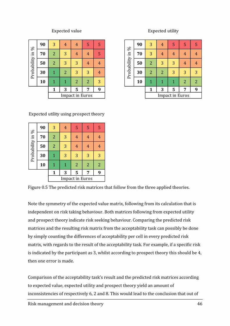
Risk management and decision theory 46
Figure 0.5 The predicted risk matrices that follow from the three applied theories.
Note the symmetry of the expected value matrix, following from its calculation that is
independent on risk taking behaviour. Both matrices following from expected utility
and prospect theory indicate risk seeking behaviour. Comparing the predicted risk
matrices and the resulting risk matrix from the acceptability task can possibly be done
by simply counting the differences of acceptability per cell in every predicted risk
matrix, with regards to the result of the acceptability task. For example, if a specific risk
is indicated by the participant as 3, whilst according to prospect theory this should be 4,
then one error is made.
Comparison of the acceptability task’s result and the predicted risk matrices according
to expected value, expected utility and prospect theory yield an amount of
inconsistencies of respectively 6, 2 and 8. This would lead to the conclusion that out of
90 3 4 4 5 5 90 3 4 5 5 5
70 2 3 4 4 5 70 3 4 4 4 4
50 2 3 3 4 4 50 2 3 3 4 4
30 1 2 3 3 4 30 2 2 3 3 3
10 1 1 2 2 3 10 1 1 1 2 2
1 3 5 7 9 1 3 5 7 9
90 3 4 5 5 5
70 2 3 4 4 4
50 2 3 4 4 4
30 1 3 3 3 3
10 1 1 2 2 2
1 3 5 7 9
Pro
bab
ility
in %
Impact in Euros
Expected value Expected utilityP
rob
abili
ty in
%
Pro
bab
ility
in %
Impact in Euros Impact in Euros
Expected utility using prospect theory

Risk management and decision theory 47
the presented decision theories, expected utility is most consistent with the
participant’s indication of acceptability of risks, followed by expected value and
prospect theory.
The conclusion of this example is that the theory that predicts the risk matrix most
accurately is prospect theory. Both expected value and prospect theory correctly
identify the highest priority risks, in accordance with the residual risk matrix. Also, the
participant behaves according to their risk matrix during the risk reducing task.
Further available information that could be analysed is data on the participant’s
demographic and socioeconomic characteristics, DOSPERT results and used
manipulations. This data can only be statistically analysed when a sufficient amount of
participants have completed the experiment.

Risk management and decision theory 48