Embed Size (px)
Citation preview
Robust Control Applied to Consistent Rendezvous
and Docking
by
Carlos Andrade
Submitted to the Department of Aeronautics and Astronauticsin partial fulfillment of the requirements for the degree of
Engineer in Aeronautics and Astronautics
at the
EPF ECOLE D’INGENIEURS
September 2008
c© Massachusetts Institute of Technology 2008. All rights reserved.
Author . . . . . . . . . . . . . . . . . . . . . . . . . . . . . . . . . . . . . . . . . . . . . . . . . . . . . . . . . . . . . .Department of Aeronautics and Astronautics
September 04, 2008
Certified by. . . . . . . . . . . . . . . . . . . . . . . . . . . . . . . . . . . . . . . . . . . . . . . . . . . . . . . . . .Dr. Alvar Saenz-Otero
Lead Scientist, SPHERES ProgramThesis Supervisor
Accepted by . . . . . . . . . . . . . . . . . . . . . . . . . . . . . . . . . . . . . . . . . . . . . . . . . . . . . . . . .Dr. Max Cerf
EADS Astrium

2
Robust Control Applied to Consistent Rendezvous and
Docking
by
Carlos Andrade
Submitted to the Department of Aeronautics and Astronauticson September 04, 2008, in partial fulfillment of the
requirements for the degree ofEngineer in Aeronautics and Astronautics
Abstract
The Synchronized Position Hold, Engage, Reorient Experimental Satellites Program(SPHERES) at the MIT Space Systems Laboratory provides research scientist witha facility to incrementally and iteratively mature estimation, control, autonomy andartificial intelligence algorithms to advance the field in Distributed Satellite Systems.This facility is located aboard the International Space Station, which allows to provestate-of-the-art GNC algorithms in a relevant 6 DOF environment.
The present thesis deals with the analysis, design and synthesis of low-authority con-trol algorithms oriented towards a consistent procedure of rendezvous and docking.This consistency radicates in the fact to archieve a maturity level which guaran-tees that the docking will be performed with a success rate higher than 90 percent.Discrete-Time Nonlinear Adaptive controllers are developed to cancel the frictioneffects in ground testing at the SSL. H∞ controllers are implemented to take intoaccount the uncertainties of the real system. Those two controllers are applied inground and into the ISS respectivelly as a milestone towards a generalized ConsistentDocking Technology.
Thesis Supervisor: Dr. Alvar Saenz-OteroTitle: Lead Scientist, SPHERES Program
3

4

e
e
e
e
e
e
e
e
e
e
e
e
e
e
e
e
e
e
e
e
e
e
e
e
e
e
e
Neither for you
5

6
Contents
1 Introduction 11
1.1 Motivation . . . . . . . . . . . . . . . . . . . . . . . . . . . . . . . . . 11
1.2 Automated Rendezvous and Docking . . . . . . . . . . . . . . . . . . 14
1.3 The Space Systems Laboratory . . . . . . . . . . . . . . . . . . . . . 15
1.4 Background . . . . . . . . . . . . . . . . . . . . . . . . . . . . . . . . 16
1.4.1 Space Technology Maturation . . . . . . . . . . . . . . . . . . 16
1.5 The SPHERES Testbed . . . . . . . . . . . . . . . . . . . . . . . . . 17
1.5.1 Internal Systems . . . . . . . . . . . . . . . . . . . . . . . . . 19
1.5.2 Control Design in the SPHERES Satellite . . . . . . . . . . . 20
1.6 Research Objectives . . . . . . . . . . . . . . . . . . . . . . . . . . . . 21
1.7 Thesis Outline . . . . . . . . . . . . . . . . . . . . . . . . . . . . . . . 21
2 Adaptive Control 23
2.1 Introduction . . . . . . . . . . . . . . . . . . . . . . . . . . . . . . . . 23
2.2 Adaptive Control . . . . . . . . . . . . . . . . . . . . . . . . . . . . . 24
2.3 Sliding Mode Control . . . . . . . . . . . . . . . . . . . . . . . . . . . 25
2.4 Adaptive Control of Nonlinear Systems . . . . . . . . . . . . . . . . . 29
2.5 Results . . . . . . . . . . . . . . . . . . . . . . . . . . . . . . . . . . . 31
2.5.1 Simulation . . . . . . . . . . . . . . . . . . . . . . . . . . . . . 31
2.5.2 Experimental Tests . . . . . . . . . . . . . . . . . . . . . . . . 35
2.5.3 Summary . . . . . . . . . . . . . . . . . . . . . . . . . . . . . 39
7
3 Robust H∞ Control 41
3.1 Introduction . . . . . . . . . . . . . . . . . . . . . . . . . . . . . . . . 41
3.2 Satellite Dynamics . . . . . . . . . . . . . . . . . . . . . . . . . . . . 41
3.3 H∞ Control . . . . . . . . . . . . . . . . . . . . . . . . . . . . . . . . 43
3.3.1 The H∞ standard problem . . . . . . . . . . . . . . . . . . . . 43
3.3.2 Characterization Theorem for Output Feedback . . . . . . . . 44
3.3.3 Mixed Sensitivity Design . . . . . . . . . . . . . . . . . . . . . 45
3.4 Results . . . . . . . . . . . . . . . . . . . . . . . . . . . . . . . . . . . 48
3.4.1 Simulation Results . . . . . . . . . . . . . . . . . . . . . . . . 48
3.4.2 Experimental Results . . . . . . . . . . . . . . . . . . . . . . . 51
3.5 Summary . . . . . . . . . . . . . . . . . . . . . . . . . . . . . . . . . 52
4 Consistent Rendezvous and Docking 55
4.1 Introduction . . . . . . . . . . . . . . . . . . . . . . . . . . . . . . . . 55
4.1.1 Consistent Docking . . . . . . . . . . . . . . . . . . . . . . . . 55
4.2 Orbital Assembly . . . . . . . . . . . . . . . . . . . . . . . . . . . . . 56
4.3 Proposed Docking Algorithm . . . . . . . . . . . . . . . . . . . . . . . 58
4.4 Experimental Results . . . . . . . . . . . . . . . . . . . . . . . . . . . 60
4.4.1 Docking Results in the Air Table . . . . . . . . . . . . . . . . 61
4.5 Docking Results on the Flat Floor . . . . . . . . . . . . . . . . . . . . 63
4.5.1 Docking Test with the PID Controller . . . . . . . . . . . . . 63
4.5.2 Docking Test with the Adaptive Controller . . . . . . . . . . . 64
4.5.3 Docking Test with the H∞ Controller . . . . . . . . . . . . . . 66
4.5.4 Summary . . . . . . . . . . . . . . . . . . . . . . . . . . . . . 68
5 Conclusions 69
5.0.5 Thesis Summary . . . . . . . . . . . . . . . . . . . . . . . . . 69
5.1 Contributions . . . . . . . . . . . . . . . . . . . . . . . . . . . . . . . 72
5.2 Future Work . . . . . . . . . . . . . . . . . . . . . . . . . . . . . . . . 73
8
List of Figures
1-1 Soyuz Spacecraft Docking with the ISS . . . . . . . . . . . . . . . . . 12
1-2 APDS Docking System aboard the Space Shuttle Discovery . . . . . . 13
1-3 Mating system aboard the ATV . . . . . . . . . . . . . . . . . . . . . 13
1-4 Subsystems included in an RVD system . . . . . . . . . . . . . . . . . 15
1-5 Discontinuity in complexity, risk, and cost at each TRL . . . . . . . . 17
1-6 The SPHERES Satellites Aboard the ISS . . . . . . . . . . . . . . . . 18
1-7 Systems description of the SPHERES satellite . . . . . . . . . . . . . 19
1-8 SPHERES satellite control loop . . . . . . . . . . . . . . . . . . . . . 20
2-1 SPHERES satellite test in the Flat Float . . . . . . . . . . . . . . . . 23
2-2 MRAC Block Diagram . . . . . . . . . . . . . . . . . . . . . . . . . . 24
2-3 Sliding mode controller with step reference input xd = 0.2 . . . . . . . 33
2-4 Sliding mode controller with reference input xd = 0.25 sin(2 π
60t)
. . 34
2-5 Adaptive controller with step reference input xd = 0.2 . . . . . . . . . 35
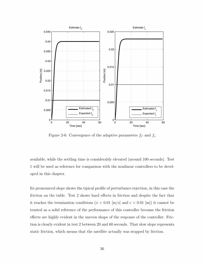
2-6 Convergence of the adaptive parameters fC and fv . . . . . . . . . . . 36
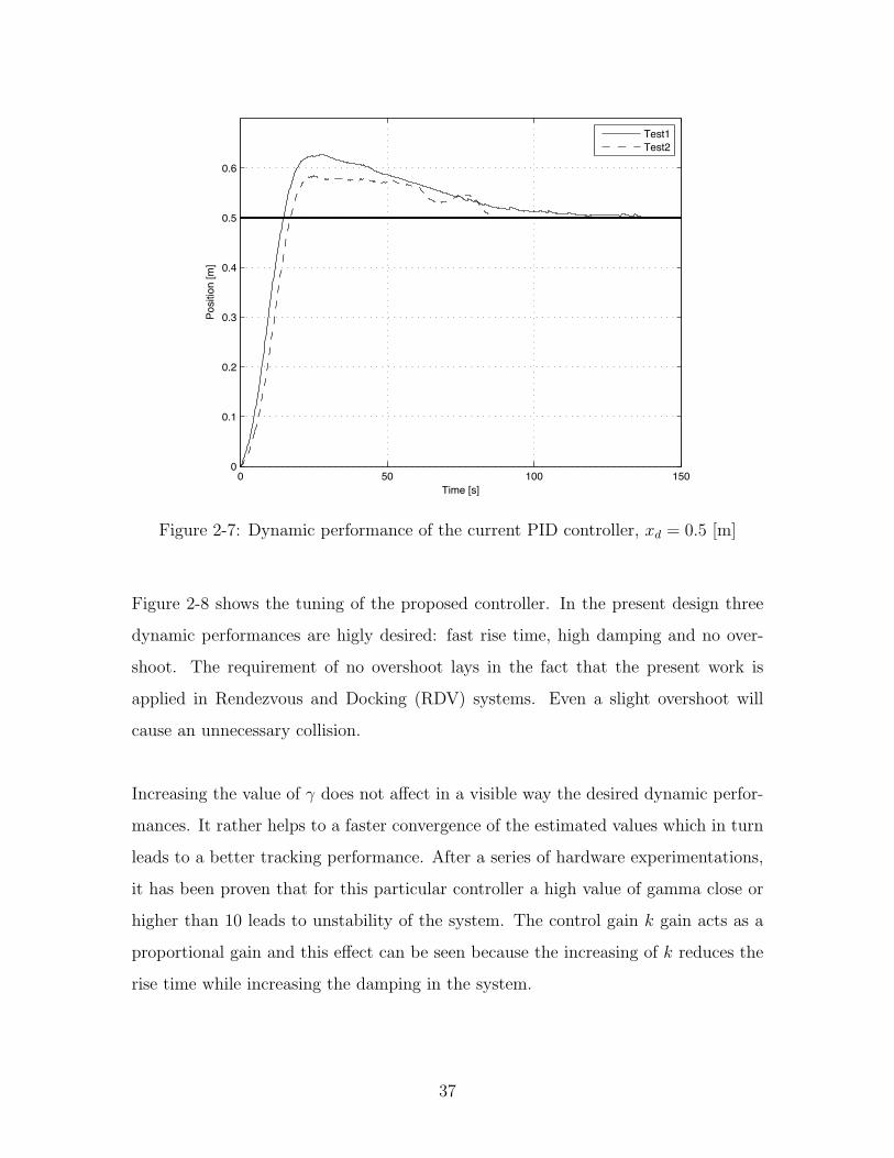
2-7 Dynamic performance of the current PID controller, xd = 0.5 [m] . . . 37
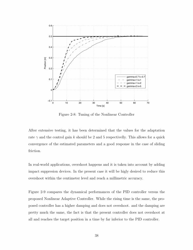
2-8 Tuning of the Nonlinear Controller . . . . . . . . . . . . . . . . . . . 38
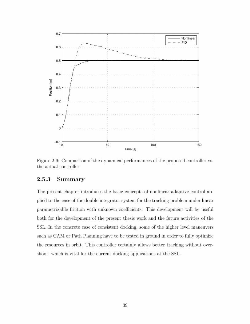
2-9 Comparison of the dynamical performances of the proposed controller
vs. the actual controller . . . . . . . . . . . . . . . . . . . . . . . . . 39
3-1 Standard H∞ Setup . . . . . . . . . . . . . . . . . . . . . . . . . . . . 43
3-2 Block Diagram for the one DOF controller . . . . . . . . . . . . . . . 46
3-3 S/KS sensitivity optimization . . . . . . . . . . . . . . . . . . . . . . 47
3-4 Magnitude Plot of W1 . . . . . . . . . . . . . . . . . . . . . . . . . . 48
9
3-5 Weighted Sensitivity Test . . . . . . . . . . . . . . . . . . . . . . . . 49
3-6 Performance Comparison. Step Input of 0.5[m] . . . . . . . . . . . . . 50
3-7 Performance Comparison. Step Input of 0.5[m] . . . . . . . . . . . . . 52
4-1 SWARM modules being tested at the MSCF flat flor . . . . . . . . . 57
4-2 SWARM Docking Port . . . . . . . . . . . . . . . . . . . . . . . . . . 58
4-3 Docking to a Fixed target Satellite Facing Backwards . . . . . . . . . 59
4-4 Docking Test with the Adaptive Controller at the Air Table . . . . . 61
4-5 Docking Test with the PID Controller at the Flat Floor . . . . . . . . 63
4-6 Step Input response of the Flat Floor Controller xd=0.5 [m] at the Flat
Floor . . . . . . . . . . . . . . . . . . . . . . . . . . . . . . . . . . . . 64
4-7 Docking test of the Adaptive Controller at the Flat Floor . . . . . . . 66
4-8 Docking Test with the H∞ controller. Tracking of the Trajectory . . . 67
10
Chapter 1
Introduction
1.1 Motivation
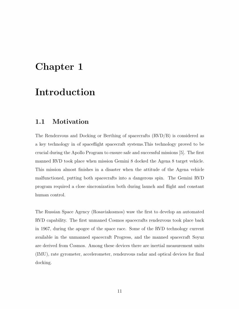
The Rendezvous and Docking or Berthing of spacecrafts (RVD/B) is considered as
a key technology in of spaceflight spacecraft systems.This technology proved to be
crucial during the Apollo Program to ensure safe and successful missions [5]. The first
manned RVD took place when mission Gemini 8 docked the Agena 8 target vehicle.
This mission almost finishes in a disaster when the attitude of the Agena vehicle
malfunctioned, putting both spacecrafts into a dangerous spin. The Gemini RVD
program required a close sincronization both during launch and flight and constant
human control.
The Russian Space Agency (Rosaviakosmos) waw the first to develop an automated
RVD capability. The first unmaned Cosmos spacecrafts rendezvous took place back
in 1967, during the apogee of the space race. Some of the RVD technology current
available in the unmanned spacecraft Progress, and the manned spacecraft Soyuz
are derived from Cosmos. Among these devices there are inertial measurement units
(IMU), rate gyrometer, accelerometer, rendezvous radar and optical devices for final
docking.
11
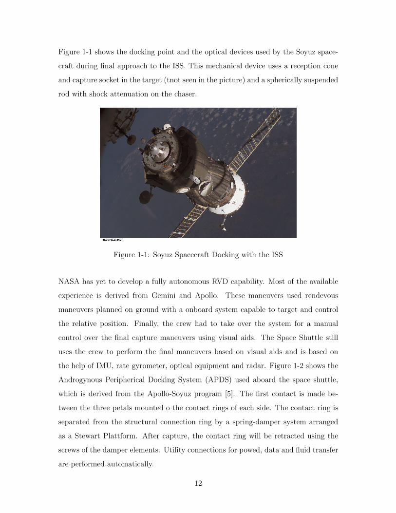
Figure 1-1 shows the docking point and the optical devices used by the Soyuz space-
craft during final approach to the ISS. This mechanical device uses a reception cone
and capture socket in the target (tnot seen in the picture) and a spherically suspended
rod with shock attenuation on the chaser.
Figure 1-1: Soyuz Spacecraft Docking with the ISS
NASA has yet to develop a fully autonomous RVD capability. Most of the available
experience is derived from Gemini and Apollo. These maneuvers used rendevous
maneuvers planned on ground with a onboard system capable to target and control
the relative position. Finally, the crew had to take over the system for a manual
control over the final capture maneuvers using visual aids. The Space Shuttle still
uses the crew to perform the final maneuvers based on visual aids and is based on
the help of IMU, rate gyrometer, optical equipment and radar. Figure 1-2 shows the
Androgynous Peripherical Docking System (APDS) used aboard the space shuttle,
which is derived from the Apollo-Soyuz program [5]. The first contact is made be-
tween the three petals mounted o the contact rings of each side. The contact ring is
separated from the structural connection ring by a spring-damper system arranged
as a Stewart Plattform. After capture, the contact ring will be retracted using the
screws of the damper elements. Utility connections for powed, data and fluid transfer
are performed automatically.
12
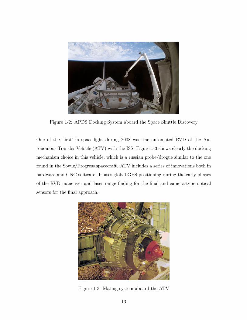
Figure 1-2: APDS Docking System aboard the Space Shuttle Discovery
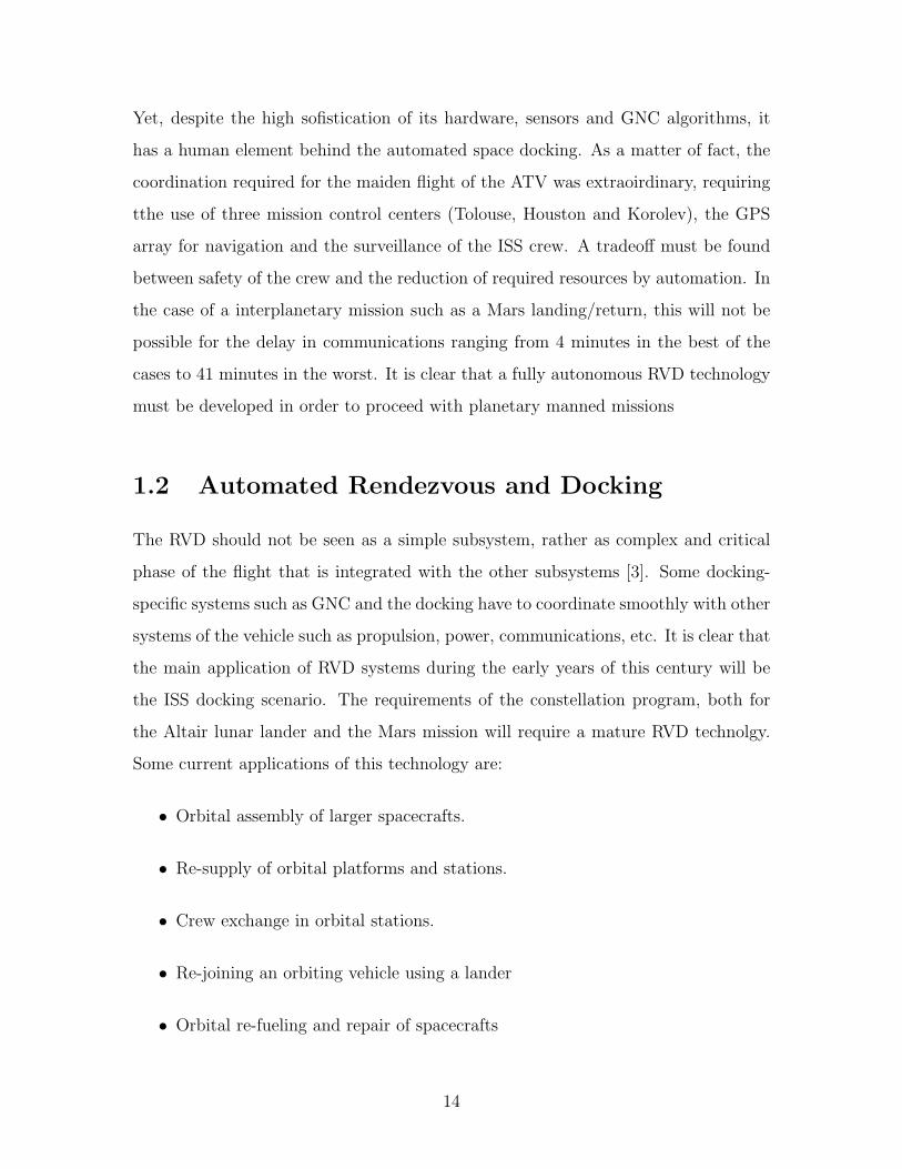
One of the ’first’ in spaceflight during 2008 was the automated RVD of the Au-
tonomous Transfer Vehicle (ATV) with the ISS. Figure 1-3 shows clearly the docking
mechanism choice in this vehicle, which is a russian probe/drogue similar to the one
found in the Soyuz/Progress spacecraft. ATV includes a series of innovations both in
hardware and GNC software. It uses global GPS positioning during the early phases
of the RVD maneuver and laser range finding for the final and camera-type optical
sensors for the final approach.
Figure 1-3: Mating system aboard the ATV
13
Yet, despite the high sofistication of its hardware, sensors and GNC algorithms, it
has a human element behind the automated space docking. As a matter of fact, the
coordination required for the maiden flight of the ATV was extraoirdinary, requiring
tthe use of three mission control centers (Tolouse, Houston and Korolev), the GPS
array for navigation and the surveillance of the ISS crew. A tradeoff must be found
between safety of the crew and the reduction of required resources by automation. In
the case of a interplanetary mission such as a Mars landing/return, this will not be
possible for the delay in communications ranging from 4 minutes in the best of the
cases to 41 minutes in the worst. It is clear that a fully autonomous RVD technology
must be developed in order to proceed with planetary manned missions
1.2 Automated Rendezvous and Docking
The RVD should not be seen as a simple subsystem, rather as complex and critical
phase of the flight that is integrated with the other subsystems [3]. Some docking-
specific systems such as GNC and the docking have to coordinate smoothly with other
systems of the vehicle such as propulsion, power, communications, etc. It is clear that
the main application of RVD systems during the early years of this century will be
the ISS docking scenario. The requirements of the constellation program, both for
the Altair lunar lander and the Mars mission will require a mature RVD technolgy.
Some current applications of this technology are:
• Orbital assembly of larger spacecrafts.
• Re-supply of orbital platforms and stations.
• Crew exchange in orbital stations.
• Re-joining an orbiting vehicle using a lander
• Orbital re-fueling and repair of spacecrafts
14
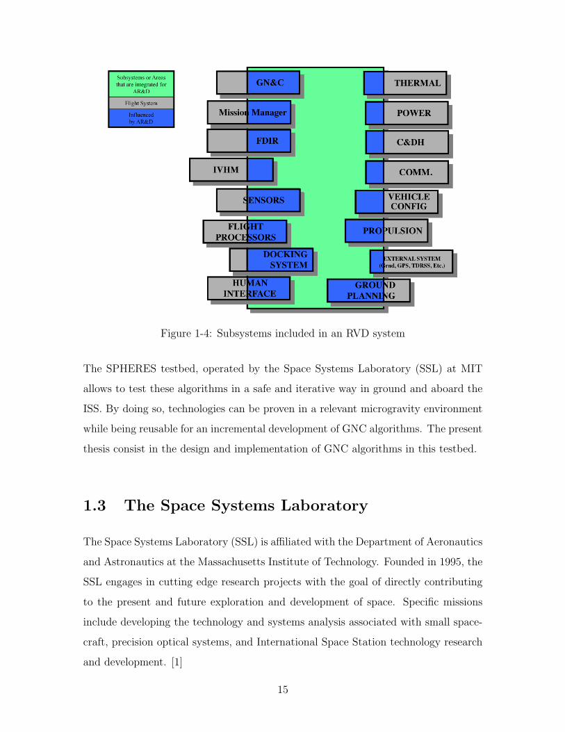
Figure 1-4: Subsystems included in an RVD system
The SPHERES testbed, operated by the Space Systems Laboratory (SSL) at MIT
allows to test these algorithms in a safe and iterative way in ground and aboard the
ISS. By doing so, technologies can be proven in a relevant microgravity environment
while being reusable for an incremental development of GNC algorithms. The present
thesis consist in the design and implementation of GNC algorithms in this testbed.
1.3 The Space Systems Laboratory
The Space Systems Laboratory (SSL) is affiliated with the Department of Aeronautics
and Astronautics at the Massachusetts Institute of Technology. Founded in 1995, the
SSL engages in cutting edge research projects with the goal of directly contributing
to the present and future exploration and development of space. Specific missions
include developing the technology and systems analysis associated with small space-
craft, precision optical systems, and International Space Station technology research
and development. [1]
15
The laboratory encompasses expertise in structural dynamics, control, thermal, space
power, propulsion, MEMS, software development and systems. A major activity in
this laboratory is the development of small spacecraft thruster systems as well as
looking at issues associated with the distribution of function among satellites. In
addition, technology is being developed for spaceflight validation in support of a new
class of space-based telescopes that exploit the physics of interferometry to achieve
dramatic breakthroughs in angular resolution. The objective of the Laboratory is to
explore innovative concepts for the integration of future space systems and to train a
generation of researchers and engineers converging in this field.
1.4 Background
1.4.1 Space Technology Maturation
One of the key aspects in the SPHERES plattform is that allows to a reliable, fault
tolerant and relative environment testbed for the development and maduration of
space technologies. Over two decades ago NASA developed the Technology Readi-
ness Levels (TRL) to determine whether a technology is ready for spaceflight. They
are a systematic measurement system that supports assessments of the maturity of
a particular technology and the consistent comparison of maturity between different
types of technology. A detailed description of TRL can be found in [13].
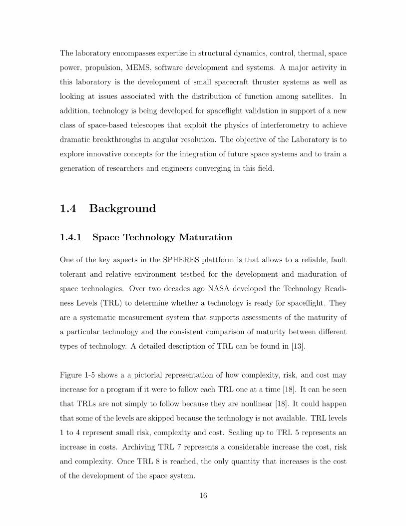
Figure 1-5 shows a a pictorial representation of how complexity, risk, and cost may
increase for a program if it were to follow each TRL one at a time [18]. It can be seen
that TRLs are not simply to follow because they are nonlinear [18]. It could happen
that some of the levels are skipped because the technology is not available. TRL levels
1 to 4 represent small risk, complexity and cost. Scaling up to TRL 5 represents an
increase in costs. Archiving TRL 7 represents a considerable increase the cost, risk
and complexity. Once TRL 8 is reached, the only quantity that increases is the cost
of the development of the space system.
16
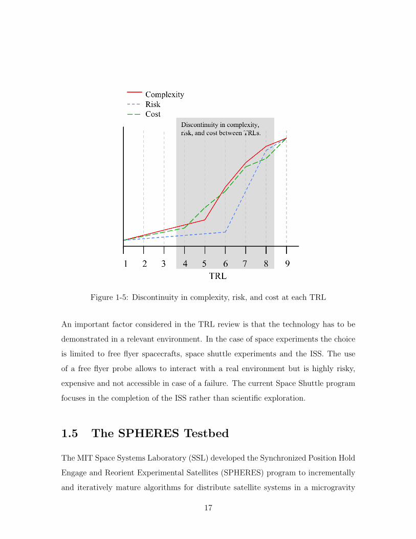
Figure 1-5: Discontinuity in complexity, risk, and cost at each TRL
An important factor considered in the TRL review is that the technology has to be
demonstrated in a relevant environment. In the case of space experiments the choice
is limited to free flyer spacecrafts, space shuttle experiments and the ISS. The use
of a free flyer probe allows to interact with a real environment but is highly risky,
expensive and not accessible in case of a failure. The current Space Shuttle program
focuses in the completion of the ISS rather than scientific exploration.
1.5 The SPHERES Testbed
The MIT Space Systems Laboratory (SSL) developed the Synchronized Position Hold
Engage and Reorient Experimental Satellites (SPHERES) program to incrementally
and iteratively mature algorithms for distribute satellite systems in a microgravity
17
environment. SPHERES is a scientific testbed specifically designed to help develop
algorithms relevant to guidance, navigation and control of spacecraft. It provides a
facility with six degrees of freedom (6 DOF) to evaluate the dynamics of a multiple
satellite system. This facility consist of a constellation of three satellites whose can
interactively communicate, maintain position, flight in formation, keep their position
and move to commanded positions as well as detect faults and run internal diagnos-
tics.
Figure 1-6: The SPHERES Satellites Aboard the ISS
The testbed is specifically designed to operate inside the International Space Station
(ISS) but they have been also successfully tested in the Reduced Gravity Aircraft
(KC-135) and in a 2D environment (3 DOF) on the flat floor at the Marshall Space
Flight Center (MSCF) and on the flat table at the SSL. A total of six satellites have
been built, tested and certified for spaceflight. Three of them are aboard the ISS
and the rest are available for ground tests and technology development prior to the
6 DOF tests aboard the ISS.
During the first year of operations with SPHERES aboard the ISS several types
of algorithms have been successfully tested aboard the International Space Station.
These algorithms include Kalman Filters, PID and glideslope control, docking al-
18
gorithms with cooperative and uncooperative targets and satellite formations. The
current lines of research include adaptive control, estimation, fault detection, intelli-
gent control, computer vision and online path planning, among several others.
1.5.1 Internal Systems
The SPHERES testbed consists of multiple micro satellites which can control their
relative positions and orientations in a 6 DOF environment. A laptop computer on-
board the ISS provided by NASA is used as a ground station to transmit commands
to the SPHERES and record telemetry. The ISS crew members use the laptop to
start tests or change test configurations.
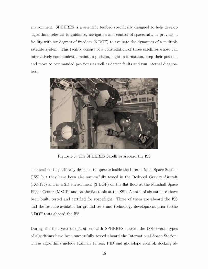
Each satellite is self-contained, with all the necessary subsystems to operate au-
tonomously Power is provided by 16 AA batteries. The propulsion system uses pres-
surized 12 CO2 miniature nozzles and electronically actuated micro-solenoid valves
(pulse-width modulation control). The position and attitude are determined using
inertial measurement units (IMU), which consist of three single axis accelerometers
and three single axis gyroscopes.
Figure 1-7: Systems description of the SPHERES satellite
19
Five ultrasonic beacons situated in the test volume provide global positioning to the
satellites. Two RF channels provide independent inter-satellite communications and
satellite-to-laptop communications. The main microprocessor is a Texas Instrument
C6701 DSP processor. ([15])
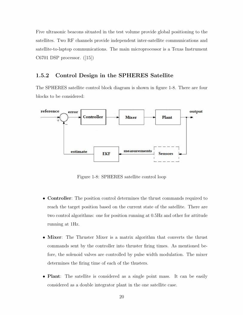
1.5.2 Control Design in the SPHERES Satellite
The SPHERES satellite control block diagram is shown in figure 1-8. There are four
blocks to be considered:
Figure 1-8: SPHERES satellite control loop
• Controller: The position control determines the thrust commands required to
reach the target position based on the current state of the satellite. There are
two control algorithms: one for position running at 0.5Hz and other for attitude
running at 1Hz.
• Mixer: The Thruster Mixer is a matrix algorithm that converts the thrust
commands sent by the controller into thruster firing times. As mentioned be-
fore, the solenoid valves are controlled by pulse width modulation. The mixer
determines the firing time of each of the thusters.
• Plant: The satellite is considered as a single point mass. It can be easily
considered as a double integrator plant in the one satellite case.
20
• Estimator: An Extended Kalman Filter (EKF) has been implemented to esti-
mate the position. The satellite’s sensors send signal to the Position and Atti-
tude Determination System (PADS) in order to estimate the position and the
satellite estimates its current position respect to a predefined reference frame.
For more precise technical information about the SPHERES testbed and its
operations, the reader might find useful to read [18], [17], [6], [14] and [16].
1.6 Research Objectives
The primary objectives of this research are summarized below:
• Demonstrate the utility of nonlinear control algorithms to compensante the
friction effects found during ground testing.
• Develop robust linear control algorithms for position control and station keep-
ing, docking and automated rendezvous.
• Integrate these control algorithms to docking maneuvers in ground to prove
assembly of in-orbit multibody spacecraft.
1.7 Thesis Outline
Chapter 2 introduces Nonlinear Adaptive Controllers to improve the accuracy of the
ground testing by compensating the contact friction. This controller is expected to
have a good dynamical performance while avoiding any overshoot and reach a static
error of less than one centimeter in order to perform a succesful docking.
Chapter 3 introduces the basic concepts in the synthesis of robust linear controllers
for position control, consistent docking and formation flight in the SISO case. H∞suboptimal controllers have been developed for position control with relative naviga-
tion by using full state knowledge.
21
Chapter 4 introduces the current concepts of RDV and shows the application of the
previous controllers as a part of this technology in different applications. The Non-
linear Adaptive Controller js applied to the SWARM project for assembly of a multi
body spacecraft. The H∞ controller will serve to show robustness in RVD algorithms
under failure.
22
Chapter 2
Adaptive Control
2.1 Introduction
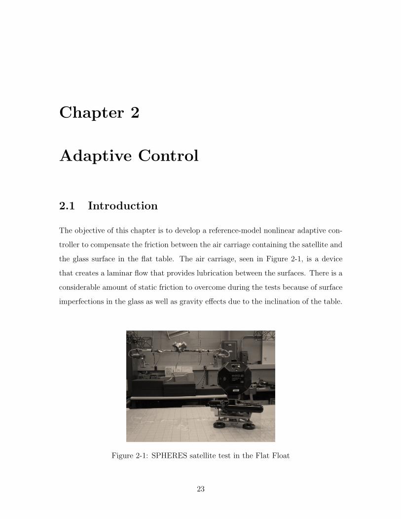
The objective of this chapter is to develop a reference-model nonlinear adaptive con-
troller to compensate the friction between the air carriage containing the satellite and
the glass surface in the flat table. The air carriage, seen in Figure 2-1, is a device
that creates a laminar flow that provides lubrication between the surfaces. There is a
considerable amount of static friction to overcome during the tests because of surface
imperfections in the glass as well as gravity effects due to the inclination of the table.
Figure 2-1: SPHERES satellite test in the Flat Float
23
2.2 Adaptive Control
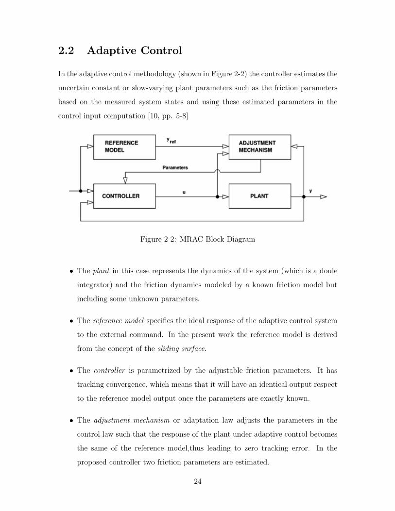
In the adaptive control methodology (shown in Figure 2-2) the controller estimates the
uncertain constant or slow-varying plant parameters such as the friction parameters
based on the measured system states and using these estimated parameters in the
control input computation [10, pp. 5-8]
Figure 2-2: MRAC Block Diagram
• The plant in this case represents the dynamics of the system (which is a doule
integrator) and the friction dynamics modeled by a known friction model but
including some unknown parameters.
• The reference model specifies the ideal response of the adaptive control system
to the external command. In the present work the reference model is derived
from the concept of the sliding surface.
• The controller is parametrized by the adjustable friction parameters. It has
tracking convergence, which means that it will have an identical output respect
to the reference model output once the parameters are exactly known.
• The adjustment mechanism or adaptation law adjusts the parameters in the
control law such that the response of the plant under adaptive control becomes
the same of the reference model,thus leading to zero tracking error. In the
proposed controller two friction parameters are estimated.
24
Two approaches were taken for the development of the proposed controller. The first
approach is the Sliding Mode control, which is an easy approach in nonlinear robust
control. However this controller often recurs to high control activity and chattering.
The other approach is the adaptive nonlinear controller, which is derived from the
sliding mode control and allows for a more precise control without chattering. In the
following sections both controllers are introduced and simulated. For practical reasons
only the adaptive nonlinear controller is implemented in the SPHERES satellites.
2.3 Sliding Mode Control
The sliding mode control is a simple approach to robust nonlinear control. It is based
in the transformation of a higher order systems into first order systems. It has been
shown [21, pp. 278-283] that tracking performance with a guaranteed precision can
be archived for these transformed problems in the presence of bounded parameter
inaccuracies while incurring in low control activity.
The particular geometric properties of the satellite allow us to make the assump-
tion that the system is a single-mass point. By doing so, the system representation
can be represented by the equations of movement:
m x = Finternal + Fexternal (2.1)
This can be rewritten for the friction problem as:
x = b u+f(x)
m(2.2)
The components of the state vector x = [x x x] represent the position, velocity
and acceleration along the direction ~x. The mass m = 13.5 [Kg] includes both the
satellite and its air carriage. The control input u represents the thrust applied in the
direction ~x. The control gain b = 1/m is known. The function f(x) represents the
estimate of the friction in the system.
25
In the present work, the Coulomb-Viscous friction model has been chosen. This
model represents well the phenomena at relativelly high velocities and stiction but
does not include presliding displacement. It can be described by the equation
f(x) = fC tanh(x
vo
)+ fvx (2.3)
The first term represents the static friction and the second term the viscous friction.
The term fC is the Coloumb friction level, fv is the coefficient of dynamical friction
and vo is the critical velocity. In the scope of this work vo=0.01 [m/s]. This value
is found recurrently on the literature for the same kind of problems (as seen in [22]
and [12]. There are other models that consider more complexe dynamics such as
the Elasto-Plastic model [4], the LuGre model or the Maxwell Generalized model [8].
However those models are not linearly parametrizable. The parameters fC and fv are
linearly parametrizable.
The friction estimate f is assumed to be bounded by a known function F = f(x, x)
such that:
|f − f | =≤ F (2.4)
where
f = −a1
(fC tanh
(x
vo
)+ fv x
)(2.5)
F = a2
(fC tanh
(x
vo
)+ fv x
)(2.6)
With a1=-0.9 and a2=1.1 are the know boundaries of the estimation error on f .
Define the target state vector as xd and the tracking error vector as x = x− xd. Let
us define a time-varying surface S(t) in the state-space R(n) by the scalar equation
s(x; t) = 0 where:
s (x; t) =
(d
dt+ λ
)x (2.7)
26
where λ is a strictly positive constant The problem of tracking x = xd is equivalent
of that of remaining on the surface S(t) for all t > 0 because s0 represents a linear
differential equation with a unique solution x0
It is shown by [21, pp. 279] that, assuming xd(0) = x(0) the tracking problem is
replaced by a first order stabilization problem in s by chosing the control law such
that ouside S(t):1
2
d
dts2 ≤ −η |s| (2.8)
Where η is a strictly positive constant that reflects the time to reach the boundary
layer starting from the outside. S(t) satisfying 2.8 is called a sliding surface. The
system’s behavoir once in S(t) is called sliding mode. Satisfying 2.8 guarantees
that if xd(0) 6= x(0), the surface S(t) will be reached in a finite time smaller than
|s(t = 0)|/η. [21, pp. 281]
The parameter s can be seen as the distance of the state of the system to the sliding
surface, which means it is an analog to the state error. It can be rewritten from its
original definition in 2.7 as:
s = x− xd + λ ˙x (2.9)
Now, including the dynamics of the system to be controlled the parameter becomes:
s = f + u− xd + λ ˙xd (2.10)
The control law estimate, u, is the best approximation to archieve s = 0 and it is
described by:
u = −f + xd − λ ˙x (2.11)
By choosing the control gain k = F + η large enough, the condition 2.8 can be met
([21],pp. 286). In order to satisfy 2.8 despite of the uncertainty in the plant dynamics
f a discontinuous term is added across the surface such that:
u = u− k sgn(s) (2.12)
27
One of the recurrent problems in sliding mode controller is chattering. One of the
easiest methods to compensate this problem is to smooth the control discontinuity in
a boundary layer of tickness φ [21, pp. 290]. This boundary layer can be implemented
as a constant layer φ=0.1. By doing so, the control law becomes:
u = u− k sat(s/φ) (2.13)
Where sat stands for the saturation of s with respect of the boundary φ. The system
performance is very sensitive to the control bandwith λ. In the present work λ is
considered to represent the neglected time delays in communications. A time delay
of TA = 400ms. is considered to take into account the communications delay between
the computer and the satellite. Taking into account the time delay is a solution
proposed in [21, pp. 302] and can be expressed as:
λ ≤ λA ≈1
3TA≈ 0.833 (2.14)
The algorithm 1 shows the proposed sliding mode controller. It receives as inputs the
state x, the target state xd and the error vector e. The output is the control command
u sent to the satellite. Finally, the values of φ and λ are constants explained earlier
in this section. The values of fc and fv are both constant values set to 0.1, which is a
value found currently in literature [8] [4]. The values of η and must be found either
by numerical optimization or by direct experimentation.
The controller developed in this section simplified because several other factors were
not taken into account. For example, the mass m=13[Kg] is supposed to be fixed,
while in reality the difference between the wet mass and the dry mass is in average
400 g. This helps to keep the mass as constant, otherwise other control gains and
time-varying boundaries must be chosen.
28
Alg. 1 ctrl pos sliding(x,xd, e). A position control algorithm to track a determined target
Input: x = [x x], xd = [xd xd], e = [e e]Output: u
1 begin2 define λ, η =, φ, fc, fv3 f = −0.9 fc tanh(x)− 0.9 fv x;4 F = 1.1 fc tanh(x) + 1.1 fv x;5 s = −e− λ e;6 k = F + η;
7 u = −f − λ e;8 u = (u− k sat(s/φ))/m;9 end
2.4 Adaptive Control of Nonlinear Systems
The adaptive control of nonlinear systems has been exploited increasingly in the last
two decades thanks to the current computational tools and recent findings in nonlinear
dynamics. This class of problems usually satisfy the following assumptions [21, pp
350]:
1. The nonlinear plant dynamics can be linearly parametrized
2. The full state is measurable
3. Nonlinearities can be canceled stably (i.e. without unstable hidden modes or
dynamics) by the control input if the parameters are known.
Once again, the single mass-point hypothesis is considered. The system can be de-
scribed by the second-order systen:
x =fCm
tanh(x
vo
)+fvmx = b u (2.15)
where the parameters fc and fv are unknown constants. The parameter b = 1/m
is a known constant. The objective of the adaptive control is to make the output
29
asymptotically track a desired output xd(t) despite the parameter uncertainty.This
can be rewritten as:
h x = fC tanh(x
vo
)+ fv x = u (2.16)
with h = 1/b = m. Let us define a combined error similar to the sliding surface
defined in 2.7:
s = e+ λ e (2.17)
where e is the position error. The scalar s can be rewritten as:
s = x− xr (2.18)
where xr, the reference value of x, is defined as:
xr = xd − λ e (2.19)
xr = xd − λ e (2.20)
The following control law is proposed [21, pp 352]:
u = h xr − k s+ fC tanh(x
vo
)+ fv x (2.21)
where k is a constant of the same sign as h. If the parameters are all known, this
choice gives exponential converge of s which in turn guarantees the convergence of e
[21, pp. 352] .For the adaptive control, the control law 2.21 is modified to include the
estimated values fC and fv
u = h xr − k s+ fC tanh(x
vo
)+ fv x (2.22)
From [21, pp. 328-329] it is posible to show that the adaptation gains can be repre-
sented by:
˙fc = − γ sgn (h) s tanh
(x
vo
)(2.23)
30
˙fv = − γ sgn (h) s x (2.24)
These adaptation gains verify global tracking convergence of the adaptive control
system. In the algorithm 2 the values of γ and are to be found by experimentation
or numerical optimization. T stands for the control period, which by convention is 2
[s] for position control in the SPHERES satellites.
Alg. 2 ctrl pos adaptive(x, xd, e). A position control algorithm to track a determinedtarget by adaptation of the friction parameters.Input: x, xd, eOutput: u
1 begin2 define λ, γ, k, T ;
3 initialize fC , fv, k, T ;4 yr = xd + λ e;5 yr = λ e;6 s = x− yrdot;
7˙fC = −γ s tanh(x);
8˙fv = −γ s x;
9 fC+ =˙fC T
10 fv+ =˙fv T
11 u = m yr − k s+ fC tanh(x) + fv x12 end
2.5 Results
2.5.1 Simulation
The controller has been tested using the discrete simulator available at the SSL, which
emulates the continuous time dynamics of the satellite while taking into account the
discrete operation of the real plant and takes into account the saturation in its actu-
ators.
31
The dynamics engine of ths simulator has been modified in order to add the non-
linear function tanh(x) described in equation 2.3 in its continuous form. This allows
to introduce the nonlinear dynamics in the simulation and emulate a more precise
environment.This function has been discretized in the controller by using a power
series expansion:
tanh(x) =5∑
n=1
B2n 4n(4n − 1)
(2n)!x2n−1 for|x| < π
2(2.25)
where Bn represents the Bernouilli numbers, whose are handily available in mathe-
matical tables.
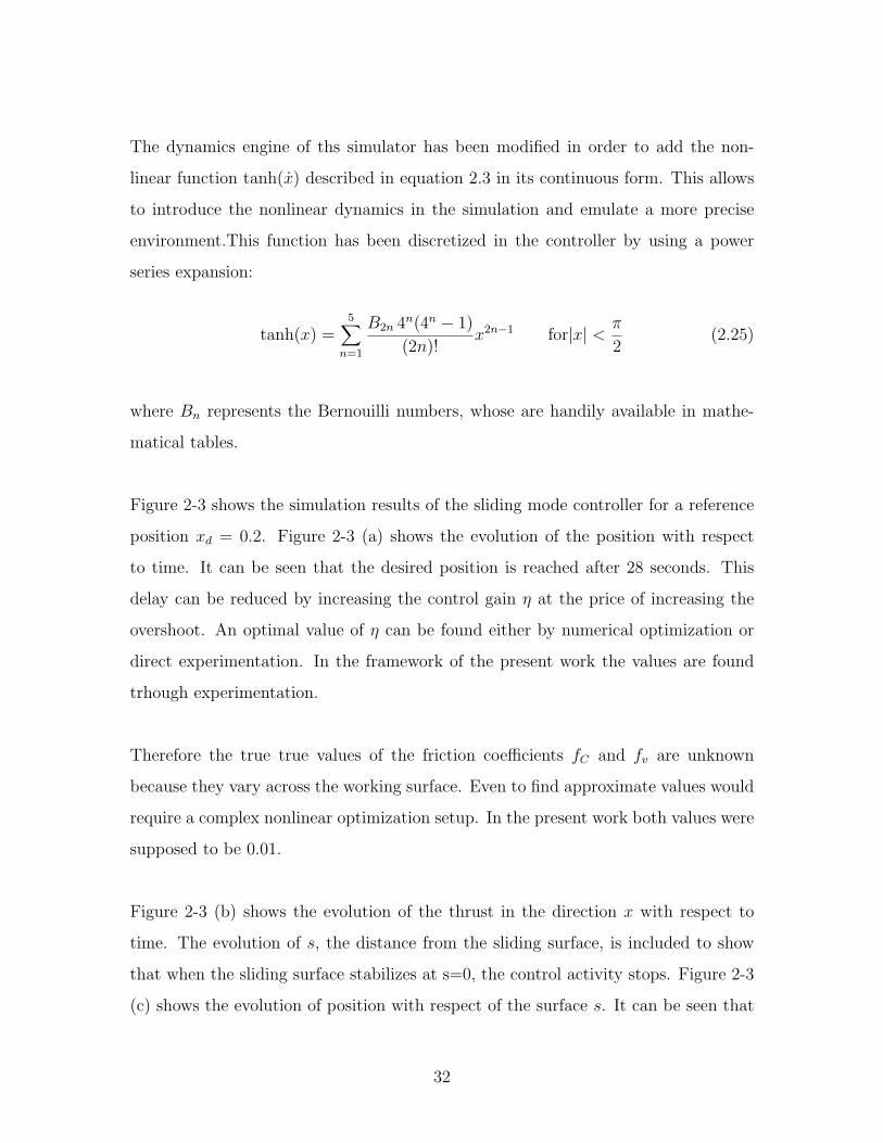
Figure 2-3 shows the simulation results of the sliding mode controller for a reference
position xd = 0.2. Figure 2-3 (a) shows the evolution of the position with respect
to time. It can be seen that the desired position is reached after 28 seconds. This
delay can be reduced by increasing the control gain η at the price of increasing the
overshoot. An optimal value of η can be found either by numerical optimization or
direct experimentation. In the framework of the present work the values are found
trhough experimentation.
Therefore the true true values of the friction coefficients fC and fv are unknown
because they vary across the working surface. Even to find approximate values would
require a complex nonlinear optimization setup. In the present work both values were
supposed to be 0.01.
Figure 2-3 (b) shows the evolution of the thrust in the direction x with respect to
time. The evolution of s, the distance from the sliding surface, is included to show
that when the sliding surface stabilizes at s=0, the control activity stops. Figure 2-3
(c) shows the evolution of position with respect of the surface s. It can be seen that
32
! "! #! $!!
!%&
!%"
!%'
!%#
()*+,-.+/0
12.)3)24,-*5.0
(67/8)49,:+.;24.+
,
,
<<=
! "! #! $!!!%"
!!%&
!
!%&
!%"
()*+,-.+/0
>26/+,-?0
(@6A.3,162B)C+
,
,
><
.
! "! #! $!!!%"
!!%&
!
!%&
!%"
!%'
()*+,-.+/0
.!.A6B7/+!12.)3)24
DE2CA3)24F,G!GA6B7/+,74=,12.)3)24
,
,
<<=
.
! "! #! $!!!%"
!!%&
!
!%&
!%"
()*+,-.+/0
.!.A6B7/+!12.)3)24
DE2CA3)24F,G!GA6B7/+,74=,12.)3)24
,
,
<<=
Figure 2-3: Sliding mode controller with step reference input xd = 0.2
when the s surface reaches zero, the state reaches its target position. Finally 2-3 (d)
shows the evolution of the tracking error, which reaches zero when s reaches 0
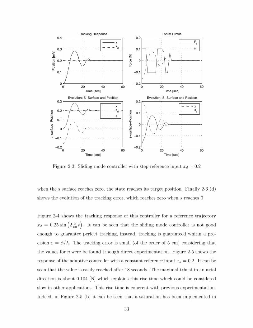
Figure 2-4 shows the tracking response of this controller for a reference trajectory
xd = 0.25 sin(2 π
60t). It can be seen that the sliding mode controller is not good
enough to guarantee perfect tracking, instead, tracking is guaranteed whitin a pre-
cision ε = φ/λ. The tracking error is small (of the order of 5 cm) considering that
the values for η were be found trhough direct experimentation. Figure 2-5 shows the
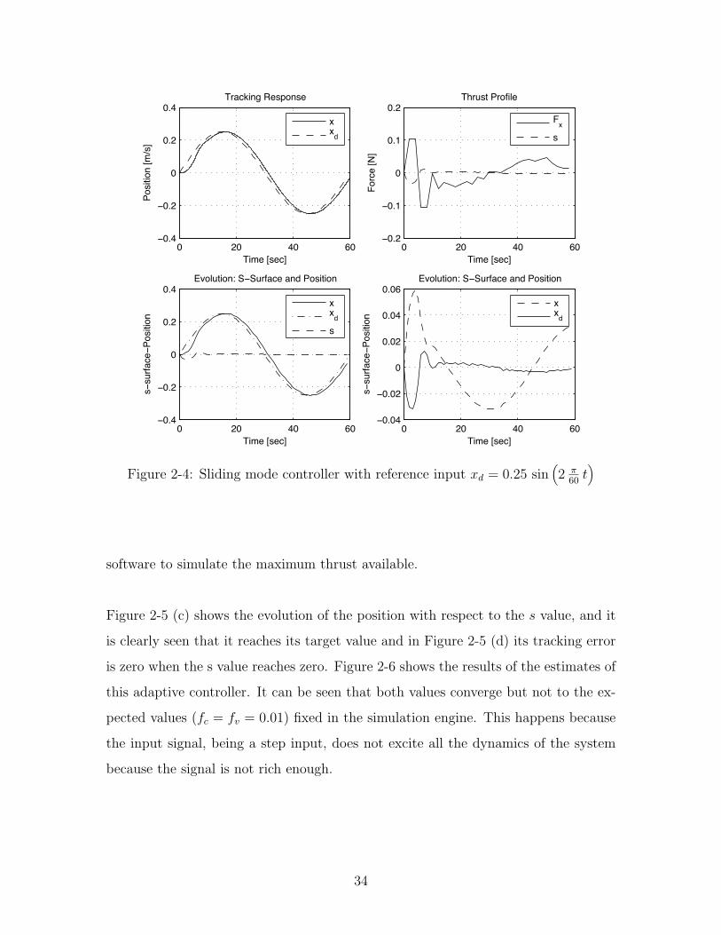
response of the adaptive controller with a constant reference input xd = 0.2. It can be
seen that the value is easily reached after 18 seconds. The maximal trhust in an axial
direction is about 0.104 [N] which explains this rise time which could be considered
slow in other applications. This rise time is coherent with previous experimentation.
Indeed, in Figure 2-5 (b) it can be seen that a saturation has been implemented in
33
0 20 40 60−0.4
−0.2
0
0.2
0.4
Time [sec]
Posi
tion
[m/s
]
Tracking Response
xxd
0 20 40 60−0.2
−0.1
0
0.1
0.2
Time [sec]
Forc
e [N
]
Thrust Profile
Fx
s
0 20 40 60−0.4
−0.2
0
0.2
0.4
Time [sec]
s−su
rface−P
ositi
on
Evolution: S−Surface and Position
xxd
s
0 20 40 60−0.04
−0.02
0
0.02
0.04
0.06
Time [sec]
s−su
rface−P
ositi
on
Evolution: S−Surface and Position
xxd
Figure 2-4: Sliding mode controller with reference input xd = 0.25 sin(2 π
60t)
software to simulate the maximum thrust available.
Figure 2-5 (c) shows the evolution of the position with respect to the s value, and it
is clearly seen that it reaches its target value and in Figure 2-5 (d) its tracking error
is zero when the s value reaches zero. Figure 2-6 shows the results of the estimates of
this adaptive controller. It can be seen that both values converge but not to the ex-
pected values (fc = fv = 0.01) fixed in the simulation engine. This happens because
the input signal, being a step input, does not excite all the dynamics of the system
because the signal is not rich enough.
34
0 20 40 600
0.05
0.1
0.15
0.2
Time [sec]
Posi
tion
[m/s
]
Tracking Response
xxd
0 20 40 60−0.2
−0.1
0
0.1
0.2
Time [sec]
Forc
e [N
]
Thrust Profile
Fx
s
0 20 40 60−0.2
−0.1
0
0.1
0.2
Time [sec]
s−su
rface−P
ositi
on
Evolution: S−Surface and Position
xxd
s
0 20 40 60−0.2
−0.1
0
0.1
0.2
Time [sec]
s−su
rface−P
ositi
on
Evolution: S−Surface and Position
es
Figure 2-5: Adaptive controller with step reference input xd = 0.2
2.5.2 Experimental Tests
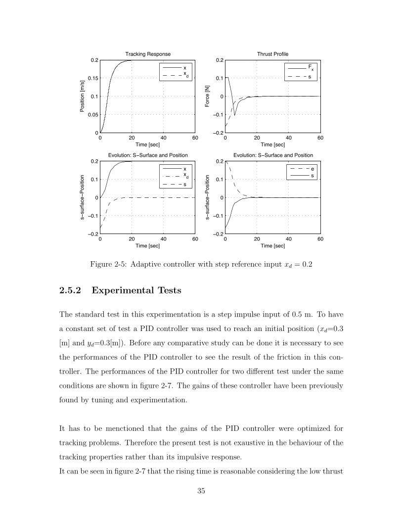
The standard test in this experimentation is a step impulse input of 0.5 m. To have
a constant set of test a PID controller was used to reach an initial position (xd=0.3
[m] and yd=0.3[m]). Before any comparative study can be done it is necessary to see
the performances of the PID controller to see the result of the friction in this con-
troller. The performances of the PID controller for two different test under the same
conditions are shown in figure 2-7. The gains of these controller have been previously
found by tuning and experimentation.
It has to be menctioned that the gains of the PID controller were optimized for
tracking problems. Therefore the present test is not exaustive in the behaviour of the
tracking properties rather than its impulsive response.
It can be seen in figure 2-7 that the rising time is reasonable considering the low thrust
35
0 20 40 600
0.005
0.01
0.015
0.02
0.025
0.03
0.035
0.04
0.045
Time [sec]
Posit
ion
[m]
Estimate fC
Estimated fCExpected fC
0 20 40 600
0.005
0.01
0.015
0.02
0.025
Time [sec]
Posit
ion
[m]
Estimate fv
Estimated fvExpected fv
Figure 2-6: Convergence of the adaptive parameters fC and fv
available, while the settling time is considerably elevated (around 100 seconds). Test
1 will be used as reference for comparison with the nonlinear controllers to be devel-
oped in this chapter.
Its pronounced slope shows the tipical profile of perturbance rejection, in this case the
friction on the table. Test 2 shows hard effects in friction and despite the fact that
it reaches the termination conditions (x < 0.01 [m/s] and e < 0.01 [m]) it cannot be
trusted as a solid reference of the performance of this controller because the friction
effects are highly evident in the uneven shape of the response of the controller. Fric-
tion is clearly evident in test 2 between 20 and 60 seconds. That slow slope represents
static friction, which means that the satellite actually was stopped by friction.
36
0 50 100 1500
0.1
0.2
0.3
0.4
0.5
0.6
Time [s]
Posit
ion
[m]
Test1Test2
Figure 2-7: Dynamic performance of the current PID controller, xd = 0.5 [m]
Figure 2-8 shows the tuning of the proposed controller. In the present design three
dynamic performances are higly desired: fast rise time, high damping and no over-
shoot. The requirement of no overshoot lays in the fact that the present work is
applied in Rendezvous and Docking (RDV) systems. Even a slight overshoot will
cause an unnecessary collision.
Increasing the value of γ does not affect in a visible way the desired dynamic perfor-
mances. It rather helps to a faster convergence of the estimated values which in turn
leads to a better tracking performance. After a series of hardware experimentations,
it has been proven that for this particular controller a high value of gamma close or
higher than 10 leads to unstability of the system. The control gain k gain acts as a
proportional gain and this effect can be seen because the increasing of k reduces the
rise time while increasing the damping in the system.
37
0 10 20 30 40 50 60 70−0.1
0
0.1
0.2
0.3
0.4
0.5
0.6
Time [s]
Posi
tion
[m]
gamma=0.7 k−0.7gamma=1 k=1gamma=1 k=2gamma=2 k=5
Figure 2-8: Tuning of the Nonlinear Controller
After extensive testing, it has been determined that the values for the adaptation
rate γ and the control gain k should be 2 and 5 respectivelly. This allows for a quick
convergence of the estimated parameters and a good response in the case of sliding
friction.
In real-world applications, overshoot happens and it is taken into account by adding
impact suppresion devices. In the present case it will be higly desired to reduce this
overshoot within the centimeter level and reach a millimetric accuracy.
Figure 2-9 compares the dynamical performances of the PID controller versus the
proposed Nonlinear Adaptive Controller. While the rising time is the same, the pro-
posed controller has a higher damping and does not overshoot. and the damping are
pretty much the same, the fact is that the present controller does not overshoot at
all and reaches the target position in a time by far inferior to the PID controller.
38
0 50 100 150−0.1
0
0.1
0.2
0.3
0.4
0.5
0.6
0.7
Time [s]
Posi
tion
[m]
NonlinearPID
Figure 2-9: Comparison of the dynamical performances of the proposed controller vs.the actual controller
2.5.3 Summary
The present chapter introduces the basic concepts of nonlinear adaptive control ap-
plied to the case of the double integrator system for the tracking problem under linear
parametrizable friction with unknown coefficients. This development will be useful
both for the development of the present thesis work and the future activities of the
SSL. In the concrete case of consistent docking, some of the higher level maneuvers
such as CAM or Path Planning have to be tested in ground in order to fully optimize
the resources in orbit. This controller certainly allows better tracking without over-
shoot, which is vital for the current docking applications at the SSL.
39

40
Chapter 3
Robust H∞ Control
3.1 Introduction
In this chapter a suboptimalH∞ robust feedback controller is developed to solve single
and multiple body trajectory tracking problems. While the ISS normally provides
the satellites a friendly environment against external perturbations and even if the
dynamic behavior of the system might be well known there exist uncertainty in the
behavior of the real system because of neglegted dynamics or physical behavior of the
subsystems.
3.2 Satellite Dynamics
Two assumptions are taken to setup the problem statement:
• H1: The satellites are considered as a single mass point.
• H2: Position and attitude dynamics are decoupled.
The equations of motion are reduced to:
m x = F (3.1)
I θ = T (3.2)
41
Where x represents the position vector x = [x y z] and F = [Fx Fy Fz] represents the
thrust vector in the axial directions. I represents the Inertia tensor and θ = [α θ ψ]
represents the angular position vector expressed in the pitch, roll and yaw angles.
T=[Tx Ty Tz] is the torque vector used in the rotational dynamics. The scope of this
work corresponds to the translational dynamics given that the rotational dynamics
are highly nonlinear and the current attitude control algorithms developed in the
SPHERES program have been found to have a good performance. Equation 3.1 can
be represented in the Laplace space L by the transfer function:
G(s) =1
s2(3.3)
This system is uncontrollable because the transfer function has two poles in the jω
axis. It is necessary to slightly perturb each of the elements of the plant as follows:
G(s) =1
(s+ ε)2(3.4)
where ε = 0.0001 is a small perturbation required to guarantee the controlability of
the system. This system can be represented as the following continuous time state-
space system:
x = Ax + BF (3.5)
y = Cx + DF (3.6)
where the minimal realization of the state matrices can be expressed as:
A =
-2x10⁻⁵ -1x10⁻⁶
0 1
B =
0
1
C =[
0 0.2326
]D = 0
(3.7)
The use of small perturbations in a second order plant is found in the literature and
does not affect the behaviour of the system [11, pp 19-321].
42
3.3 H∞ Control
3.3.1 The H∞ standard problem
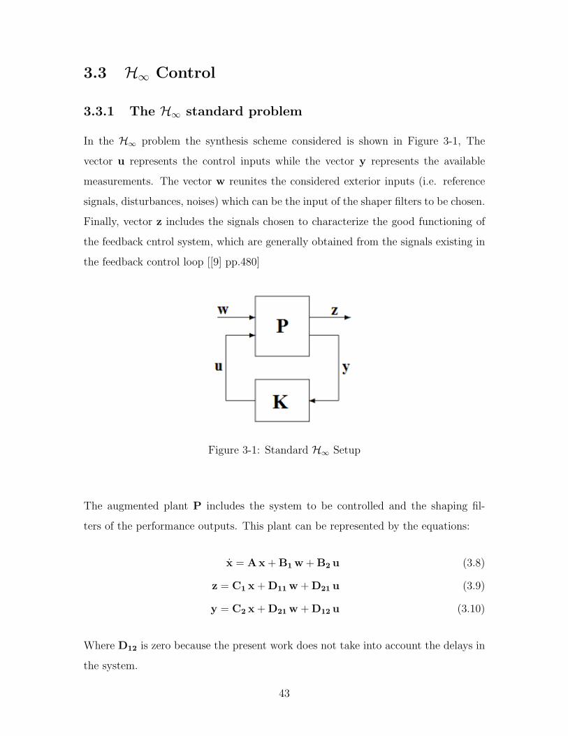
In the H∞ problem the synthesis scheme considered is shown in Figure 3-1, The
vector u represents the control inputs while the vector y represents the available
measurements. The vector w reunites the considered exterior inputs (i.e. reference
signals, disturbances, noises) which can be the input of the shaper filters to be chosen.
Finally, vector z includes the signals chosen to characterize the good functioning of
the feedback cntrol system, which are generally obtained from the signals existing in
the feedback control loop [[9] pp.480]
Figure 3-1: Standard H∞ Setup
The augmented plant P includes the system to be controlled and the shaping fil-
ters of the performance outputs. This plant can be represented by the equations:
x = Ax + B1 w + B2 u (3.8)
z = C1 x + D11 w + D21 u (3.9)
y = C2 x + D21 w + D12 u (3.10)
Where D12 is zero because the present work does not take into account the delays in
the system.
43
The augmented plant P can be also represented by its compact matrix representation:
P =
A B1 B2
C1 D11 0
C2 D21 D22
(3.11)
The optimal H∞ problem is to find all admissible controllers K(s) which minimize
the H∞ norm of the feedback system, i.e. all admissible controllers that minimize
‖P (s)‖∞. The norm ‖‖∞ can be physically seen as a measurement of the energy
performance of the system, i.e. the energy gain from input u to the output y ([7])
and is described by:
‖P (s)‖∞ = supw∈R
√λ(P (jw)P (−jw)T (3.12)
Finding an optimal controller is difficult and the optimal controllers for the H∞ prob-
lem are not unique. They can be viewed as the limit case for suoptimal controllers
and are not explicitly constructed. In this section, the suboptimal H∞ problem is
considered. The suboptimal H∞ controller K(s) is found for a given γ > 0 when
‖P (s)∞‖ < γ. The optimization problem consist in finding a value γopt such that, for
any admissible controller:
γopt = inf {‖P (s)| ∞ } (3.13)
For γ = γopt there are no suboptimal controllers. A controller is said to be admissible
if it stabilises internally the system P (s) and it is proper, i.e. the vector D in the
system 3.1 is zero.
3.3.2 Characterization Theorem for Output Feedback
The H∞ suboptimal controllers assume the following properties:
44
(A1) (A,B1) is stabilizable and (C1,A) is detectable.
(A2) (A,B2) is stabilizable and (C2,A) is detectable.
(A3) DT12 C1=0 and DT
12 D12=I
(A4) B1 DT21=0 and D21 DT
21=I
(A5) D11=0 and D22=0
It can be seen ([11], pp. 165-170) that the previous asumptions are sufficient condition
for the stability of P (s) and the internal stability of the closed-loop system. In fact
(A1), (A3) and (A4) imply that the feedback loop is internally stable if and only if
G(s) ∈ H∞. The existence of the H∞ controllers via Riccati equations can be easily
found in the classical textbooks such as [11], [20] and [23] and therefore it is ommited
here.
3.3.3 Mixed Sensitivity Design
The proposed methodology is to pose the H∞ standard problem using a mixed sensi-
tivity desing. For doing so, the original plan G is mathematically extended by using
shaping weights that contain the design goals of the system. These weights usually
have the form of a nth order filter. The extended plant is denoted by P.
The sensitivity function is a semi-proper transfer function with an infinite H2 norm.
This function represents the closed loop transfer function from the output distur-
bances to the outputs. The proposed controller in Fig. 3-2 is an one degree of
freedom (DOF) controller which can be shapen to have better dynamic performances
or perturbance rejection characteristics but not both at the same time. The following
terminology is introduced ([20]):
L = GK (3.14)
S = (I + GK)−1 = (I + L)−1 (3.15)
T = (I + GK)−1GK = (I + L)−1L (3.16)
45
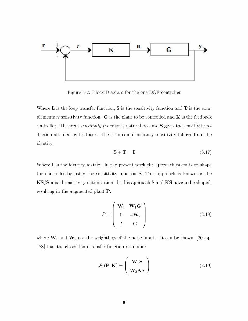
Figure 3-2: Block Diagram for the one DOF controller
Where L is the loop transfer function, S is the sensitivity function and T is the com-
plementary sensitivity function. G is the plant to be controlled and K is the feedback
controller. The term sensitivity function is natural because S gives the sensitivity re-
duction afforded by feedback. The term complementary sensitivity follows from the
identity:
S + T = I (3.17)
Where I is the identity matrix. In the present work the approach taken is to shape
the controller by using the sensitivity function S. This approach is known as the
KS/S mixed-sensitivity optimization. In this approach S and KS have to be shaped,
resulting in the augmented plant P:
P =
W1 W1G
0 −W2
I G
(3.18)
where W1 and W2 are the weightings of the noise inputs. It can be shown [[20],pp.
188] that the closed-loop transfer function results in:
Fl (P,K) =
W1S
W2KS
(3.19)
46
In the present work, the control input filter W2 has been chosen to be equal to
1, or I in the multivariable case. This helps to simplify the model. A common filter-
ing suggested by [2] and [20] for the performance output filter W1 is:
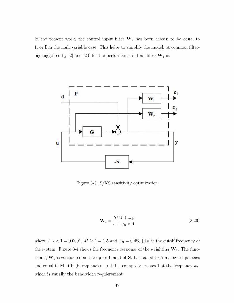
Figure 3-3: S/KS sensitivity optimization
W1 =S/M + ωBs+ ωB ∗ A
(3.20)
where A << 1 = 0.0001, M ≥ 1 = 1.5 and ωB = 0.483 [Hz] is the cutoff frequency of
the system. Figure 3-4 shows the frequency response of the weighting W1. The func-
tion 1/W1 is considered as the upper bound of S. It is equal to A at low frequencies
and equal to M at high frequencies, and the asymptote crosses 1 at the frequency wb,
which is usually the bandwidth requierement.
47
10−5
10−4
10−3
10−2
10−1
100
101
102
−10
0
10
20
30
40
50
60M
agni
tude
(dB)
Bode Diagram
Figure 3-4: Magnitude Plot of W1
3.4 Results
3.4.1 Simulation Results
The experimental methodology chosen is similar to the one applied in the previous
chapter. The satellite will move to the position xd = 0.3 [m] and yd = 0.3 [m] at zero
velocity with a PID controller. Once this start position is reached the controller is
tested by switching controllers and having as its new target xd = 0.8
One of the objectives in the synthesis of a H∞ controller is to reach γopt = 1. This
is not a crucial objective, rather it is a design goal. The synthesis of the controller
hereby developed reached a value of γ = 1.4801. This can be seen in Figure 3-5. In
a ideal controller the sensitivity function S is expected to not surpass the function
1/W1. Once again, this characteristic is not critical and the values of the weights
were selected in function of the performance of the controller in the discrete-time
SPHERES dynamics simulator.
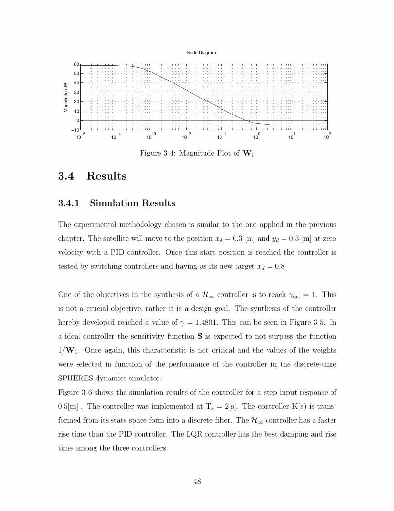
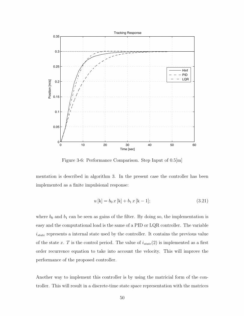
Figure 3-6 shows the simulation results of the controller for a step input response of
0.5[m] . The controller was implemented at Ts = 2[s]. The controller K(s) is trans-
formed from its state space form into a discrete filter. The H∞ controller has a faster
rise time than the PID controller. The LQR controller has the best damping and rise
time among the three controllers.
48
−1 0 1 2
−0.6
−0.5
−0.4
−0.3
−0.2
−0.1
0
0.1
Freq (rad/sec)
Mag
nitu
de
S1/W
s
WsS
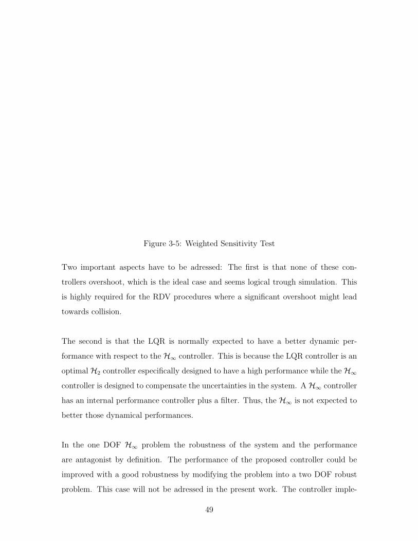
Figure 3-5: Weighted Sensitivity Test
Two important aspects have to be adressed: The first is that none of these con-
trollers overshoot, which is the ideal case and seems logical trough simulation. This
is highly required for the RDV procedures where a significant overshoot might lead
towards collision.
The second is that the LQR is normally expected to have a better dynamic per-
formance with respect to the H∞ controller. This is because the LQR controller is an
optimal H2 controller especifically designed to have a high performance while the H∞controller is designed to compensate the uncertainties in the system. A H∞ controller
has an internal performance controller plus a filter. Thus, the H∞ is not expected to
better those dynamical performances.
In the one DOF H∞ problem the robustness of the system and the performance
are antagonist by definition. The performance of the proposed controller could be
improved with a good robustness by modifying the problem into a two DOF robust
problem. This case will not be adressed in the present work. The controller imple-
49
0 10 20 30 40 50 600
0.05
0.1
0.15
0.2
0.25
0.3
0.35
Time [sec]
Posit
ion
[m/s
]
Tracking Response
HinfPIDLQR
Figure 3-6: Performance Comparison. Step Input of 0.5[m]
mentation is described in algorithm 3. In the present case the controller has been
implemented as a finite impulsional response:
u [k] = b0 x [k] + b1 x [k− 1]; (3.21)
where b0 and b1 can be seen as gains of the filter. By doing so, the implementation is
easy and the computational load is the same of a PID or LQR controller. The variable
istate represents a internal state used by the controller. It contains the previous value
of the state x. T is the control period. The value of istate(2) is implemented as a first
order recurrence equation to take into account the velocity. This will improve the
performance of the proposed controller.
Another way to implement this controller is by using the matricial form of the con-
troller. This will result in a discrete-time state space representation with the matrices
50
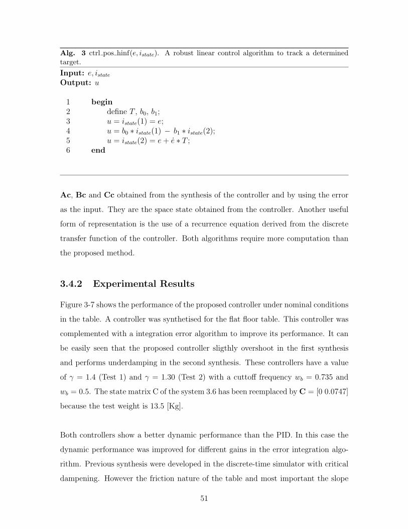
Alg. 3 ctrl pos hinf(e, istate). A robust linear control algorithm to track a determinedtarget.Input: e, istateOutput: u
1 begin2 define T , b0, b1;3 u = istate(1) = e;4 u = b0 ∗ istate(1) − b1 ∗ istate(2);5 u = istate(2) = e+ e ∗ T ;6 end
Ac, Bc and Cc obtained from the synthesis of the controller and by using the error
as the input. They are the space state obtained from the controller. Another useful
form of representation is the use of a recurrence equation derived from the discrete
transfer function of the controller. Both algorithms require more computation than
the proposed method.
3.4.2 Experimental Results
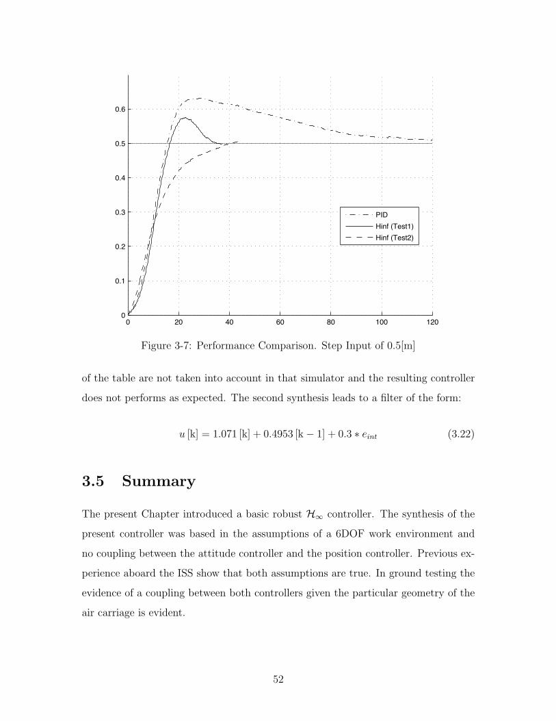
Figure 3-7 shows the performance of the proposed controller under nominal conditions
in the table. A controller was synthetised for the flat floor table. This controller was
complemented with a integration error algorithm to improve its performance. It can
be easily seen that the proposed controller sligthly overshoot in the first synthesis
and performs underdamping in the second synthesis. These controllers have a value
of γ = 1.4 (Test 1) and γ = 1.30 (Test 2) with a cuttoff frequency wb = 0.735 and
wb = 0.5. The state matrix C of the system 3.6 has been reemplaced by C = [0 0.0747]
because the test weight is 13.5 [Kg].
Both controllers show a better dynamic performance than the PID. In this case the
dynamic performance was improved for different gains in the error integration algo-
rithm. Previous synthesis were developed in the discrete-time simulator with critical
dampening. However the friction nature of the table and most important the slope
51
0 20 40 60 80 100 1200
0.1
0.2
0.3
0.4
0.5
0.6
PIDHinf (Test1)Hinf (Test2)
Figure 3-7: Performance Comparison. Step Input of 0.5[m]
of the table are not taken into account in that simulator and the resulting controller
does not performs as expected. The second synthesis leads to a filter of the form:
u [k] = 1.071 [k] + 0.4953 [k− 1] + 0.3 ∗ eint (3.22)
3.5 Summary
The present Chapter introduced a basic robust H∞ controller. The synthesis of the
present controller was based in the assumptions of a 6DOF work environment and
no coupling between the attitude controller and the position controller. Previous ex-
perience aboard the ISS show that both assumptions are true. In ground testing the
evidence of a coupling between both controllers given the particular geometry of the
air carriage is evident.
52
A modified H∞ controller for the air table is described. For this particular case
an error integration algorithm was added to the proposed controller in order to reach
the final position. This controller was developed as a way to demonstrate the imple-
mentation of the H∞ controller proposed in this work. Only flight experience will
show whether the H∞ controller has accomplished its objectives.
53

54
Chapter 4
Consistent Rendezvous and
Docking
4.1 Introduction
Rendezvous and docking or berthing (RVD /B) is a key operational technology, re-
quired for many missions involving more than one spacecraft. Control techniques have
been successfully implemented in the automated rendezvous and docking of space-
crafts requiring some degree of manual control. However, when the uncertainty of the
system increases the performance of RVD /B may diminish to unacceptable levels
with potential mission failures. The testing of new technologies such as the AVGS
navigation proposed in the DART mission [19] are too expensive to fail.
4.1.1 Consistent Docking
The idea of Consistent Docking comes to answer the problem of RVD aiming towards
fully autonomy of the process. This includes the integration of several algorithms pre-
viously developed or in development at the SSL such as path planning, fault detection,
plume imprigment, collision avoidance, position and attitude controllers, among oth-
ers. The key contribution of the present work is the addition of the adaptive nonlinear
and robust linear controllers with application in grond and space respectivelly.
55
The complete automation of the rendevouz procedures are crucial in the next phases
of space exploration. As menctioned in the introduction of the present work, there will
not be real-time manned surveillance capability for any RVD maneuver executed in a
planetary mission because of the delays in communication. Besides, this technology
can be applied for the servicing of satellites and space probes without the intervention
of astronauts. With the retiring of the Space Shuttle any manned satellite servicing
other than the Hubble servicing mission is discarded in the near future.
The criteria of success expected in this technology for purpose research at the SSL
is to have a safe automated docking with a 90 percent of success as a starting point,
despite the evolving nature of the space environment. The ISS allows to develop the
required GNC algorithms iteratively in a relevant environment and with a certain
safety in case of failure.
Two applications are foreseen in the framework of the present work. The first is
the development of docking procedures for the ground testing of the SWARM mod-
ular spacecraft concept. This will be explained in the next section. The second
application is the testing of docking procedures aboard the ISS and the study of the
response of these docking procedures under a unexpected thruster failure.
4.2 Orbital Assembly
One of the concepts being curently explored at the SSL is the Self-assembling, Wire-
less, Autonomous, Reconfigurable Modules (SWARM). This is an innovative approach
to modular fabrication and in-space robotic assembly of large scale systems. The
SWARM concept uses formation flown spacecraft, containing multiple universal dock-
ing ports (Figure 4-2) whose serve to dock with modular elements and maneuver them
to dock with other similar elements.
56
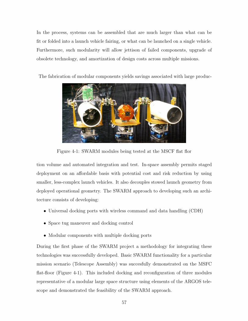
In the process, systems can be assembled that are much larger than what can be
fit or folded into a launch vehicle fairing, or what can be launched on a single vehicle.
Furthermore, such modularity will allow jettison of failed components, upgrade of
obsolete technology, and amortization of design costs across multiple missions.
The fabrication of modular components yields savings associated with large produc-
Figure 4-1: SWARM modules being tested at the MSCF flat flor
tion volume and automated integration and test. In-space assembly permits staged
deployment on an affordable basis with potential cost and risk reduction by using
smaller, less-complex launch vehicles. It also decouples stowed launch geometry from
deployed operational geometry. The SWARM approach to developing such an archi-
tecture consists of developing:
• Universal docking ports with wireless command and data handling (CDH)
• Space tug maneuver and docking control
• Modular components with multiple docking ports
During the first phase of the SWARM project a methodology for integrating these
technologies was successfully developed. Basic SWARM functionality for a particular
mission scenario (Telescope Assembly) was succesfully demonstrated on the MSFC
flat-floor (Figure 4-1). This included docking and reconfiguration of three modules
representative of a modular large space structure using elements of the ARGOS tele-
scope and demonstrated the feasibility of the SWARM approach.
57
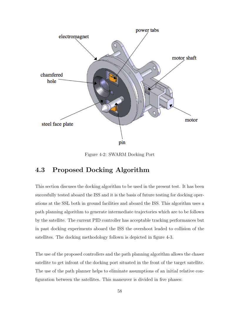
Figure 4-2: SWARM Docking Port
4.3 Proposed Docking Algorithm
This section discuses the docking algorithm to be used in the present test. It has been
succesfully tested aboard the ISS and it is the basis of future testing for docking oper-
ations at the SSL both in ground facilities and aboard the ISS. This algorithm uses a
path planning algorithm to generate intermediate trajectories which are to be follown
by the satellite. The current PID controller has acceptable tracking performances but
in past docking experiments aboard the ISS the overshoot leaded to collision of the
satellites. The docking methodology follown is depicted in figure 4-3.
The use of the proposed controllers and the path planning algorithm allows the chaser
satellite to get infront of the docking port situated in the front of the target satellite.
The use of the path planner helps to eliminate assumptions of an initial relative con-
figuration between the satellites. This maneuver is divided in five phases:
58
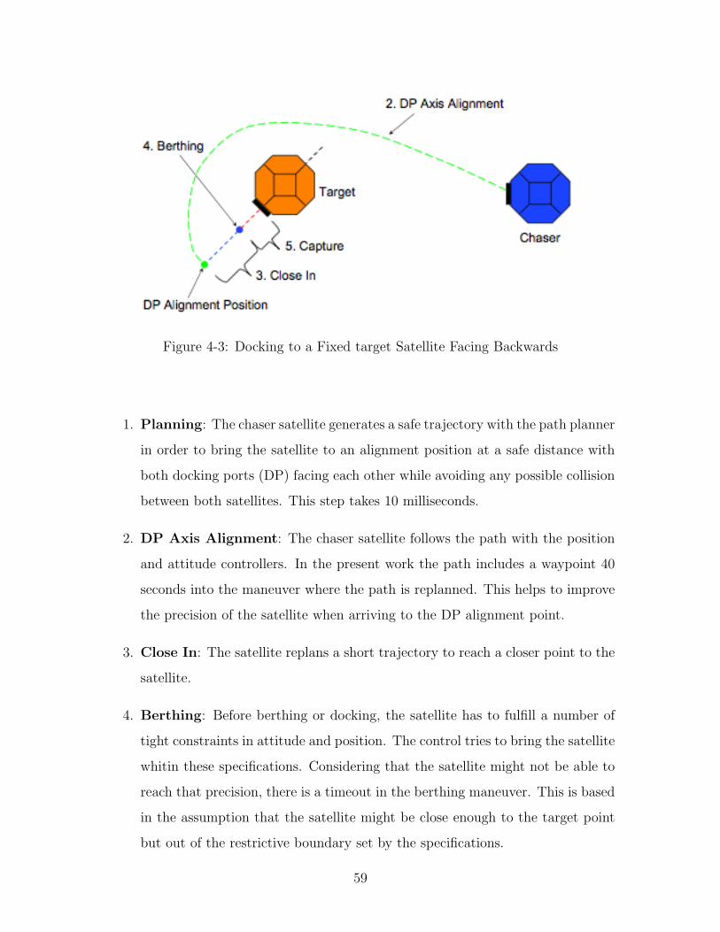
Figure 4-3: Docking to a Fixed target Satellite Facing Backwards
1. Planning: The chaser satellite generates a safe trajectory with the path planner
in order to bring the satellite to an alignment position at a safe distance with
both docking ports (DP) facing each other while avoiding any possible collision
between both satellites. This step takes 10 milliseconds.
2. DP Axis Alignment: The chaser satellite follows the path with the position
and attitude controllers. In the present work the path includes a waypoint 40
seconds into the maneuver where the path is replanned. This helps to improve
the precision of the satellite when arriving to the DP alignment point.
3. Close In: The satellite replans a short trajectory to reach a closer point to the
satellite.
4. Berthing: Before berthing or docking, the satellite has to fulfill a number of
tight constraints in attitude and position. The control tries to bring the satellite
whitin these specifications. Considering that the satellite might not be able to
reach that precision, there is a timeout in the berthing maneuver. This is based
in the assumption that the satellite might be close enough to the target point
but out of the restrictive boundary set by the specifications.
59
5. Capture: The chaser satellite moves towards its target and both docking port
enter into contact.
Given the restrictive nature of the berthing conditions there is a good possibility that
the maneuver fails. The SPHERES satellites aboard the ISS use velcro as a safe,
inexpensive solution that allows to explore docking maneuvers. Some problems arise,
such as plume impingement and hard contact with the chaser. These problems will
not be adressed in the framework of the present thesis.
In the case of ground procedures the problem becomes harder because of surface
imperfections. Even considering an adaptive controller the surface might have irregu-
larities that can easily lead the testing hardware in the wrong direction. At the time
of the writing of this thesis the 6 DOF test aboard the ISS haven’t been run because
of factors out of the author’s control. The following results will focus extensivelly on
the ground work rather than the ISS research which hopefully will be performend in
the early fall.
4.4 Experimental Results
The results described in this section include the air table at the SSL laboratory and
the flat floor. The flat floor facility provides researchers with a bigger surface for
experiments, in comparison with the limited surface on the air table (about 1.5 [m2]).
The proposed experimental methodology for the automated docking maneuver is the
following:
• Both satellites are put in front of each other, ibetween 70-100 centimeters. Both
docking ports are facing each other.
• The chaser satellite will adjust its attitude to align both docking ports. In this
test the target satellite has been set to keep position.
• The chaser satellite follows the path, reaches the waypoint and replans the new
path.
60
• After following the close-in path the satellite reaches the berthing position. It
stays there until the position error is less than 5 millimeters or it reaches its
timeout after 60 seconds in this maneuver.
• Finally, once the conditions are fullfilled or a timeout happens the chaser satel-
lite moves towards the target satellite. If succesfully executed, this maneuver
should dock both satellites within a tolerance of 1 cm.
4.4.1 Docking Results in the Air Table
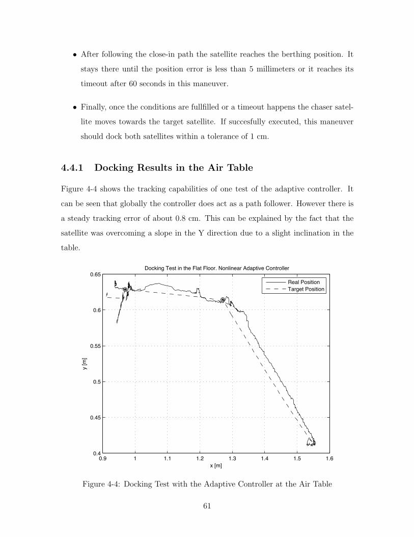
Figure 4-4 shows the tracking capabilities of one test of the adaptive controller. It
can be seen that globally the controller does act as a path follower. However there is
a steady tracking error of about 0.8 cm. This can be explained by the fact that the
satellite was overcoming a slope in the Y direction due to a slight inclination in the
table.
0.9 1 1.1 1.2 1.3 1.4 1.5 1.60.4
0.45
0.5
0.55
0.6
0.65Docking Test in the Flat Floor. Nonlinear Adaptive Controller
x [m]
y [m
]
Real PositionTarget Position
Figure 4-4: Docking Test with the Adaptive Controller at the Air Table
61
The nonlinear controller does not handle well the slope at this point. The black dots
show the waypoints generated by the path planner. The controller reach the way-
points and performs well the final approach. Even given that the controller does not
meet the berthing conditions, it reach the docking point within the tolerances. In the
experiment shown above the position error at the point of contact was 0.64 [cm]. This
allows a docking whitin the tolerance. This tolerance appears from the specific design
of the docking port shown previously in figure 4-2. The hole for the pin is 2.5 cm wide.
Being withing 1 [cm] will allow the satellite to be well inside the chanferred area
of the hole, so even if the internal hole is just 1 [cm] in diameter, the chmamfered
hole will contain the pin. Harware implementation of the docking port will be left as
future work because the path planner requieres to be reconfigured. At this point the
path planner considers its default docking face the -X plane of the satellite, which
contains the velcro face. Future work will include adding the current version of the
docking port which includes its own metrology system that can be used for close range
tracking. By doing so, the precision at the contact point and the contact velocity can
be handled more precisely than with the global metrology used throughout this thesis.
Another explanation of the tracking error can be the non-optimality of the gains
used. Optimal gains specified for the tracking problem will lead to a better tracking
precision and reach safely the docking port. Finally, the lack of accuracy in the fric-
tion model has to be taken into account. The Coloumb-Viscous model does not take
into account pre-sliding deplacement, which can be unexpectedly present across the
table in the form of a scratch or a surface irregularity. This can be handle with the
internal state models, whose take that part into account but are strictly nonlinearly
parametrizable.
62
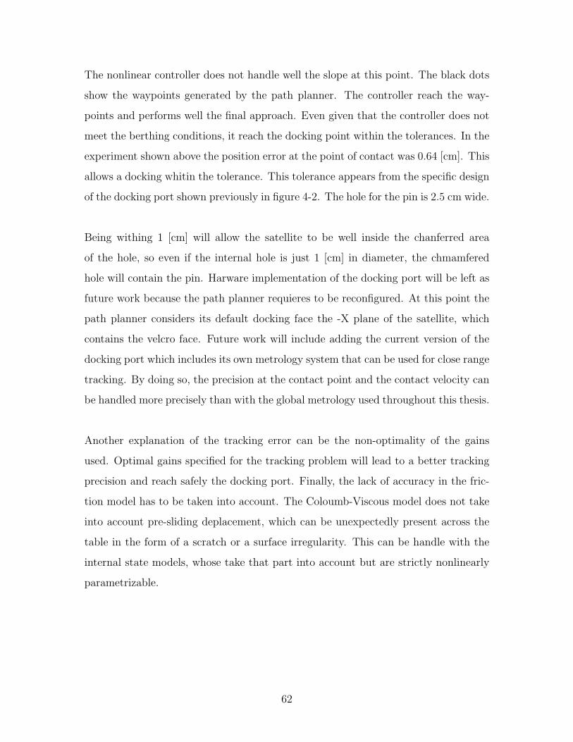
4.5 Docking Results on the Flat Floor
4.5.1 Docking Test with the PID Controller
The use of the flat floor provides scientist the opportunity of working with a broader
range of experiments that were not viable in the reduced surface of the air carriage.
However the friction characteristics are not the same. As a matter of fact, the control
of the satellite with the air carriage in the flat floor is a more complex task given that
the uneveness of the surface is more important. Figure 4-5 shows the response of the
current PID controller in a docking experiment.
0.3 0.35 0.4 0.45 0.5 0.55 0.6 0.650.04
0.05
0.06
0.07
0.08
0.09
0.1
0.11
0.12
0.13
0.14Docking Test in the Flat Floor. PID Controller
x [m]
y [m
]
Real PositionTarget Position
Figure 4-5: Docking Test with the PID Controller at the Flat Floor
The tracking is good overall but the control activity is really demanding for the satel-
lite. This means a huge use of resources such as CO2 for the propulsion and batteries
for the soneloids in the nozzels. The controller starts to diverge before reaching the
first waypoint.
63
The path shape can be explained by a reconfiguration made by the path planner
because of a existent timeout of 60 seconds between the start of the test and the way-
point.the controller still tries to track the new path and reaches the berthing position.
However, while the controller is in the berthing position integrates the error and this
results in a completelly wrong contact point. In the experiment shown above the PID
controller misses the target by more than 5 centimeters.
4.5.2 Docking Test with the Adaptive Controller
Figure 4-6 shows some experiments run in the finding of the new gains for the adap-
tive controller. It can be seen that the PID controller has a static error of around 9
cm.
0 20 40 60 80 100 1200
0.1
0.2
0.3
0.4
0.5
0.6
Time [s]
Posit
ion
[m]
Step Input Test in the Flat Floor with xd=0.5 [m]
PIDNonlinear (Test1)Nonlinear (Test2)
Figure 4-6: Step Input response of the Flat Floor Controller xd=0.5 [m] at the FlatFloor
64
The particular shape of the control response in this case responds to the fact that
the satellite reached an uneven surface and it was unable to overcome, the thrust
level required sent to the satellite by the PID controller do not overcome the friction
effects. The flat surface in the response plot means that the controller is overcoming
the friction slowly.
The first experiment with the nonlinear controller (Test1, in figure 4-6 shows that
by using h the controller gain k=10 and the adaptation rate γ=3 has a slow rising
time and does reach the target position at the end, having a slight overshoot of two
centimenters.The second experiment (Test2) shows that a synthesis with k=20 and
γ=3 and it overshoots slightly but does reach the target position.
Nevertheless a more precise model of the friction has to be taken into account given
the fact that the presliding friction effects are not taken into account in the curent
model. This leads to unexpected performances of the controller in some tracking test.
It has to be stated that both the adaptation rate and the control gain have not been
found by numerical optimization. This could help to reach an optimal performance for
tracking problems. This optimization is not treated in the framework of the present
work. These values are found trough direct experimentation and their performance
has been evaluated in considering both tracking error, steady state error, overshoot
and rise time.
Figure 4-7 shows the docking results of the adaptive controller at the Flat Floor
using γ=3 and k=10. This controller does not perform very well in the tracking
performance. At the time of the writing of this work the exact values for parameters
of the adaptive controller at the Flat Floor haven’t been found. It has to be stated
that the scale of this plot shows a big error on the tracking. However the final error
is actually 2.2 [cm].
65
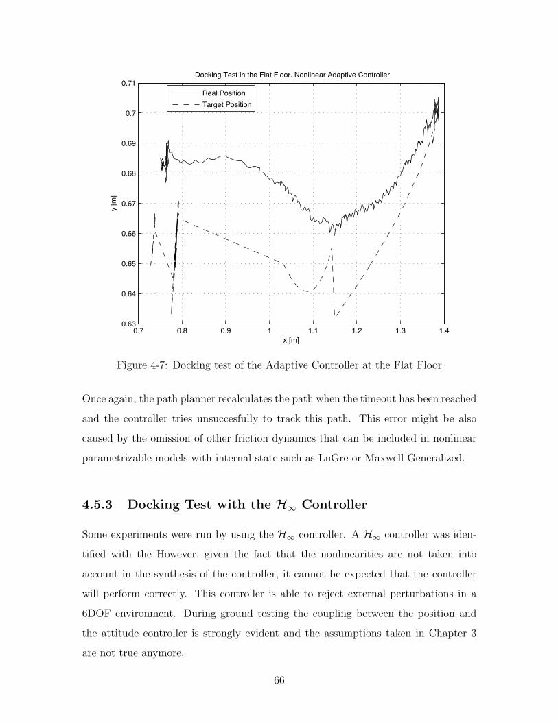
0.7 0.8 0.9 1 1.1 1.2 1.3 1.40.63
0.64
0.65
0.66
0.67
0.68
0.69
0.7
0.71
x [m]
y [m
]
Docking Test in the Flat Floor. Nonlinear Adaptive Controller
Real PositionTarget Position
Figure 4-7: Docking test of the Adaptive Controller at the Flat Floor
Once again, the path planner recalculates the path when the timeout has been reached
and the controller tries unsuccesfully to track this path. This error might be also
caused by the omission of other friction dynamics that can be included in nonlinear
parametrizable models with internal state such as LuGre or Maxwell Generalized.
4.5.3 Docking Test with the H∞ Controller
Some experiments were run by using the H∞ controller. A H∞ controller was iden-
tified with the However, given the fact that the nonlinearities are not taken into
account in the synthesis of the controller, it cannot be expected that the controller
will perform correctly. This controller is able to reject external perturbations in a
6DOF environment. During ground testing the coupling between the position and
the attitude controller is strongly evident and the assumptions taken in Chapter 3
are not true anymore.
66
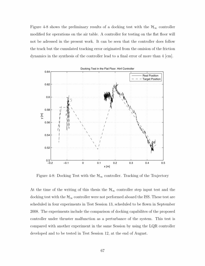
Figure 4-8 shows the preliminary results of a docking test with the H∞ controller
modified for operations on the air table. A controller for testing on the flat floor will
not be adressed in the present work. It can be seen that the controller does follow
the track but the cumulated tracking error originated from the omision of the friction
dynamics in the synthesis of the controller lead to a final error of more than 4 [cm].
−0.2 −0.1 0 0.1 0.2 0.3 0.4 0.50.5
0.52
0.54
0.56
0.58
0.6
0.62
0.64
x [m]
y [m
]
Docking Test in the Flat Floor. Hinf Controller
Real PositionTarget Position
Figure 4-8: Docking Test with the H∞ controller. Tracking of the Trajectory
At the time of the writing of this thesis the H∞ controller step input test and the
docking test with theH∞ controller were not performed aboard the ISS. These test are
scheduled in four experiments in Test Session 13, scheduled to be flown in September
2008. The experiments include the comparison of docking capabilites of the proposed
controller under thruster malfunction as a perturbance of the system. This test is
compared with another experiment in the same Session by using the LQR controller
developed and to be tested in Test Session 12, at the end of August.
67
The other test to be flown aboard the ISS as a part of the present work include
also a comparison of the tracking performance of the proposed controller with respect
of the PID and the LQR controller in the same maneuver. The maneuver chosen is
the path tracking of a Spiral maneuver. Figure ?? shows the tracking performance
of the proposed test based on simulation. It can be seen that the LQR is the best
tracking controller with a final error of 6 cm. The PID controller has a final error of
12 cm and the H∞ controller has a final error of 10 cm. This was expected because
the H∞ controller is not specified for performance and it is expected to have a infe-
rior performance with respect of the H∞ controller. In the other hand, the proposed
controller has a better performance if compared with the PID controller and this is
only for tracking problems.
4.5.4 Summary
The present chapter explored diverse experiments with the docking maneuvers by
using different controllers. The test were run by using the PID, Nonlinear Adaptive
and H∞ controllers. Given that these test were run in a frictioning workspace it was
the logical result that the nonlinear adaptive controller is evidently the best solution.
The PID controller has been extensively used in the past because of the madurity of
that control. It is expected that with time the nonlinear adaptive controller becomes
the standard controller for ground testing at the SSL.
In overall the adaptive controller does well its work of friction compensation. However
it has been seen that tracking performance is an issue to be adressed. Mathematical
optimization will bring important feedback to reach an optimal controller with exce-
lent tracking capabilities.
The case of perturbance rejection has not been adressed in this work. Test Ses-
sion 13 will bring invaluable data in the proposed H∞ test performed in a relevant
environment. This leads to a incremental work for Test Session 14 where other robust
linear controllers will be developed aiming towards decentralized control.
68
Chapter 5
Conclusions
5.0.5 Thesis Summary
The present work has shown the development of robust nonlinear and linear con-
trollers and their application to flight formation task. These controllers can be used
in any formation flight, docking or multi body spacecraft maneuvering for the ground
test and space flight cases respectivelly. The objective of the present thesis was to
strongly pursue the use of the proposed controllers towards a fully consisted auto-
mated rendezvous and docking of the satellites. The development of the proposed
controllers is another increasing task of many others to be developed in order to full-
fill a real consisted RVD algorithm tested under extreme operational conditions in a
relevant environment.
Chapter 2 proposes an adaptive nonlinear controller to compensate the friction during
ground testing. The metrics evaluated to measure the improvement of this controller
with respect to the previous PID controller were no overshoot, no static error and a
fast rise time without incurring in overshoot. This controller has been proven to be
succesful in basis of the metrics imposed and considering the step input test. The
step input test is a standard test in control analysis and design. However this control
should be modified for specific applications. In particular, the tracking performance
of the proposed controller has to be improved.
69
Overshoot happens in the controllers on the flat floor. This is required because the
gains had been increased to overcome a friction that experimentally has been proven
to be more challenging that the work at the air table. Even with the optimal gains
found trough mathematical optimization, there is a fair amount of work to be done
in order to At the time of the writing of this thesis his controller has been succesfully
used in applications other than docking. However tracking must be improved given
the fact that tracking error is a metric to be considered in several other applications
such as star navigation or interferometry.
In Chapter 3 H∞ control is introduced as an approach of how to deal with uncer-
tainties. The deveopment of the present controller is a first step in the way of more
complex robust algorithms. Robust lineal control is a topic not well explored in the
current level of the SPHERES program. The ATV mission shown that perturbance
rejection in LEO and in approach/berthing/docking can be done in a more efficient
way that other controllers such as Eigenvalue Assignment and PID [19]. In the case
of a robust lineal controller for spaceflight in a outer space environment, mathemat-
ical computation might increase and the dynamics of the perturbation have to be
linearized. Other solution is to use a complex LTV lineal synthesis. This work is yet
to be done at least for the case of fully automated docking procedures
H∞ is a technique not often used in spaceflight because of the risk that it might
imply to use a new technology and because of the madurity of the present techniques.
With the computational power of onboard calculators increasing and a better under-
standing of the space environment, the H∞ applications in space flight environment
will increase with time.
The robust controller has not been tested aboard the ISS by the time of the writting
of the present thesis. The present year has seen an important activity in the construc-
tion of the orbital outpost. Test Session 12 has been postponed several times and
it will bring invaluable data from docking test with LQR algorithms during August
70
30th, 2008. TTest Session 13, to be flown not earlier than September 6th, 2008, will
validate the same algorithm under thruster malfunction and using the proposed H∞Controller. Also, the tracking performance of the proposed controller will be tested
by using a three-satellites spiral algorithm where each of the satellites has a different
controlller.
While the H∞ accounts for the parametric uncertainty of unmodeled dynamics, the
LQR is better performant. A tradeoff must be found in the selected application. The
use of a 2DOF H∞ controller must lead to better dynamical performances while in-
creasing the robustness of the system. The selected metric for the H∞ test is rejection
perturbance. So far simulations show a better rejection perturbance than the PID
controller. However this simulation does not take into account all the dynamics and
therefore is not conclusive. Flight data will pave the road for the improvement of the
proposed H∞ controller.
Chapter 4 shows the use of both controllers to the docking maneuvers. The pro-
posed docking architecture shown in Chapter 4 has been succesfully used at the ISS
beign the first docking experiment with a path planner used on orbit. The path plan-
ner has proven to be a helpful resource for this architecture. However, as it has been
seen in previous experiments, the low level controllers must be improved to better
the tracking capabilities and avoid overshooting. The use of LQR controllers aboard
the ISS for docking purposes will bring a insight on which performances are required
for the docking problem.
In the case of ground operations the nonlinear adaptive controller has ben tested
extensively in the air table. The work in the flat floor is fairly new. Tests in the air
table are most of the time succesfuls but still there is a fair amount of work to do
if a more complex dynamica model has to be included (multi body problem) or if
a new friction model is to be considered. In that case, the present synthesis is not
valable anymore and a new nonlinear adaptive controller has to be designed unless
71
the nonlinearities are linearized The docking algorithms H∞ controller will be tested
aboad the ISS in the early fall 2008. Simulation has shown the feasibility of this con-
troller and the potential success of the mission to be flown. However, as it happens
more often than aerospace enginners would like, errors can happen. Therefore only
until the results come from the ISS it can be stated that the developed controller is
succesful and has fullfilled its objectives
5.1 Contributions
The most important contributions of the thesis work hereby present are related with
the area of robust control. Both nonlinear controllers and robust linear controllers
have been developed in the framework of this thesis. One of the key points in the
work hereby presented is a high performance nonlinear controller which will
be the standard position controller during ground testing at the SSL not
only for the SPHERES projects and for future aplications.
The robust controller hereby proposed is expected to be the cornerstone of a con-
sistent docking algorithm. This technology is in development and it will take a long
time to have a full in-space tested version of this consistent docking algorithm The
robust controller is expected to assure the robustness of the system despite
the neglected satellite dynamics given the simplifications taken in the synthesis
of the proposed controller. Besides, it is highly difficult to have an accurate model
of the whole system with uncertainties derived from continuos-time dynamics of the
actuators and discrete-time delays from communication and data processing.
Finally, the key contribution of the present work is the development of controllers
and the use of existent docking algorithms to prove the ability to conduct a con-
sistent docking in ground with a success rate superior than 90 percent .
At this point this capability has been reached in the air table. Work in the optimal
This is key for the testing of the SWARM program to be done during the winter of
72
2008 at the Marshall Space Flight Center in Alabama.
5.2 Future Work
The nonlinear controller still can be improved. Some problems have been seen during
the pre-sliding displacement, this is self-correcting given the nature of the proposed
control algorithm. Other nonlinear parametrizable models such as LuGre or Elasto-
Plastic might help to solve this problem.
From the operational point of view, the proposed controller has fullfilled the expec-
tations. In the case of continuous breaking algorithms such as stop-and-stare control
algorithms proposed for satellite imagery, this might be a problem that will be need
to be adressed.
The nonlinear controller has proven to be an almost ideal controller for the proposed
task (milimeter-precision control with friction compensation). Experience shows that
this controller works fine under several surface discontinuities. Yet, there are other
dynamical characteristics that are to be improved, such as presliding displacement.
The present work shows that the proposed controller is far superior to the actual
controllers developed in the SSL for the ground testing. In the past, members of
the SPHERES team hesitated to fully verify their algorithms in the 2-DOF facility
because of the well known friction and gravitational effects.
Hopefully, the proposed controller will lead to a new culture of full testing before
the orbital testing and even more: to test new technology with hardware in develop-
ment, such as the case of the SWARM project.
It is clear that a lot of work remains left in the current docking technologies available
at the SSL. In comparison of the space agencies or the big companies, the solutions
proposed at the SSL must be viable technically and economically. Other docking
73
technologies might be suggested such as optical devices, visual-based navigation and
pattern recognition. Also. It has to be stated that the current facility at the ISS
has only the velcro faces as an emulation of this docking port. Ideally, in the future,
SPHERES might be upgraded with these docking ports already developed.
This would lead to a fully hardware-in-the-loop autonomous docking of spacecrafts,
which lead to a important contribution in the field by adding a series of maneuver-
ing conditions such as CAM maneuvers, obstacle avoidance, uncooperative docking,
thumbing docking and others that already have been adressed by other researchers at
the SSL but have to be proven with real docking hardware. It is important to recall
that the problem of docking is challenging for both hardware design and software
design. Both must be tested in order to reach a fully demonstrated docking ability.
Limitations in time did not allowed to have a full analysis of robustness and un-
certainties on the H∞ controller . Future work will be required on this subject to
take into account thruster saturation, uncertainties in the thrusters and noise from
the sensors.
74
Bibliography
[1] Mit space systems lab. http://ssl.mit.edu/about/. Last acces: August 18th,2008.
[2] I. Bates, D. Postlehwaite. Robust Multivariable Control of Aerospace Systems.Number 08 in Control and Simulation. DUP Science, 2002.
[3] N. Currie. Advancing technology and education for an human base on the moonand mars. Presentation to the Engineering Dean’s Conference, October 2006.
[4] P. Dupont, B. Armstrong, and .V Hayward. Elasto-plastic friction model: Con-tact compilance and stiction. In Proceedings of the American Control Conference,volume 2, pages 1072–1076, Chicago, IL, March 2000.
[5] W. Fehse. Automated Rendezvous and Docking of Spacecraft. CambridgeAerospace Series. Cambridge Univertsity Press, Cambridge, UK, 2003.
[6] M. Hilstad. A multi-vehicle testbed and interface framework for the developmentand verification of separated spacecraft control algorithms. Master’s thesis, Mas-sachusetts Institute of Technology, June 2005.
[7] J. How. Principles of optimal control. Lecture Notes, 2003.
[8] V. Lampaert, F. Al-Bender, and J. Swevers. A generealized maxwell-slip frictionmodel appropiate for control purposes. In Proceedings of the Physics and Con-trol Conference PHYSCON 2003, volume 1, pages 1170–1176, Moscow, Russia,August 2003.
[9] P.de Larminat, editor. Analysys and Control of Lineal Systems. 2003.
[10] W. Li. Adaptive Control for Robot Motion. PhD thesis, Massachusetts Instituteof Technology, May 1990.
[11] U. Mackenroth. Robust Control Systems: Theory and Case Studies. Springer-Verlag, 2004.
[12] C. Makkar, . W. E. Dixon, W.G. Sawyer, and G. Hu. A new continuouslydifferentiable friction model for control systems design. In Proceedings of the 2005IEEE/ASME International Conference on Advanced Intelligent Mechatronics,volume 1, pages 600–605, Monterey, CA, July 2005. IEEE/ASME.
75
[13] J. Mankins. Technology readiness levels. Technical report, Advanced ConceptsOffice, Office of Space Access and Technology, NASA, April 1995.
[14] S. Nolet. Development of a Guidance, Navigation and Control Architecture andValidation Process Enabling Autonomous Docking to a Tumbling Satellite. PhDthesis, Massachusetts Institute of Technology, June 2007.
[15] S. Nolet, E. Kong, and D.W. Miller. Autonomous docking algorithm developmentand experimentation. volume 5149. SPIE, 2004.
[16] S. Nolet, A. Saenz-Otero, D.W. Miller, and A. Fejzic. Spheres operations aboardthe iss: Maturation of gnc algorithms in microgravity. 2007.
[17] A. Saenz-Otero. The spheres satellite formation flight testbed: Design and initialcontrol. Master’s thesis, Massachusetts Institute of Technology, August 2000.
[18] A. Saenz-Otero. Design Principles for the Development of Space TechnologyMaturation Laboratories Aboard the International Space Station. PhD thesis,Massachusetts Institute of Technology, June 2005.
[19] N. Silva, M. Ganet, E. Goribus, and P. Augros. Autonomous rendezvous: Guid-ance and control in elliptical orbit. In AIIA Guidance, Navigation and ControlConference and Exibit, volume 1, Hilton Head, SC, August. AIAA.
[20] S. Skogestad and I. Postlethwaite. Multivariable Feedback Control: Analysis andDesign. Wiley, 1996.
[21] Li W. Slotine, J-J. Applied Nonlinear Control. Prentice Hall, 1991.
[22] S. Thiery, M. Kunze, A. Karimi, A. Curnier, and R. Longchamp. Friction mod-eling of a high precision positioning system. In Proceedings of the 2006 AmericanControl Conference, volume 1, pages 1863–1867, June 2006.
[23] K. Zhou, J. Doyle, and K. Glover. Robust and Optimal Control. Prentice Hall,1995.
76