Embed Size (px)
Citation preview
RTG 1666 GlobalFood ⋅ Heinrich Düker Weg 12 ⋅ 37073 Göttingen ⋅ Germany www.uni-goettingen.de/globalfood
ISSN (2192-3248)
www.uni-goettingen.de/globalfood
RTG 1666 GlobalFood
Transformation of Global Agri-Food Systems: Trends, Driving Forces, and Implications for Developing Countries
Georg-August-University of Göttingen
GlobalFood Discussion Papers
No. 63
Financial literacy and food safety standards in Guatemala: The heterogeneous impact of GlobalGAP on farm income
Anna K. Müller
Ludwig Theuvsen
February 2015
Financial literacy and food safety standards in Guatemala: The heterogeneous impact of GlobalGAP on
farm income
Anna K. Müller*; Ludwig Theuvsen
Georg-August University Göttingen, Department of Agricultural Economics and Rural Development, Research Training Group “Transformation of the global agri-food system – Trends, driving forces and implications for developing countries”
*corresponding author: [email protected]
Abstract
The transformation of the global agrifood system is characterized by the increasing
importance of food safety and quality standards. This trend is challenging farmers in
countries like Guatemala, who often lack necessary skills and assets. We contribute to
the ongoing discussion about the impact of standards on smallholder farmers by
considering impact heterogeneity. By using propensity score matching techniques, we
show that farmers with a higher level of financial literacy seem to benefit more from
standard adoption than those with lower levels of financial literacy. Our results hold
important practical implications for exporters, standard setters and development
organizations.
Keywords: Food safety standards, financial literacy, developing countries, impact analysis, propensity score matching, impact heterogeneity
JEL Codes: Q14, Q12, Q16, O33, C31, I26
We gratefully acknowledge the support of the DFG (Deutsche Forschungsgemeinschaft)
and Stiftung Fiat Panis. Special thanks go to IFPRI and GlobalGAP for providing
secondary data.
2
1. Introduction
With the transformation of the global agri-food system, the role of organizational and
process innovations in global agricultural value chains is gaining importance. The
dominance of process related standards (public and private) that are applied in
agricultural production and farm management is one characteristic of the ongoing
dynamics.1 There is a lot of discussion in development research and practice about the
impact of the increasing standardization of agriculture on small farmers in developing
countries. Two scenarios are discussed. First, it is argued that the increasing
requirements on food quality and safety might challenge already marginalized producers
in countries with weak quality infrastructure. Due to high compliance costs and missing
capacities and skills, farmers might not be able to comply with the new requirements.
This could lead to negative socioeconomic effects with consequences for rural poverty.
The second scenario is more optimistic. It sees positive upgrading effects with benefits
for farmers and the agricultural sector in general. The more stringent requirements could
induce upgrading activities in the agricultural sector, helping farmers to increase
productivity, decrease production costs, improve quality and safety and thus gain better
access to international high-value chains and receive better prices and higher
agricultural incomes.
Studies examining the economic impact of adopting food quality standards generally
find that doing so has a positive effect (Asfaw et al. 2009; Holzapfel and Wollni 2014;
Hansen and Trifković 2014b; Subervie and Vagneron 2013; Handschuch et al. 2013).
This overall positive effect stems from special price arrangements, quality
improvements, the use of contracts, tighter supplier-buyer relationships, and higher
efficiency in farm input use. But even between certified farmers, the economic impact
can vary with the institutional arrangements (Holzapfel and Wollni 2014), access to
infrastructure (Subervie and Vagneron 2013) and/or farm size (Hansen and Trifković
2014). Capital endowment, access to resources and information, and farmer’s capacities
1 Standards like GlobalGAP address processes on the farm level, i.e. they require new pest management strategies, record keeping for traceability issues and specific training for the farmer and any farm employees. Process standards are an organizational innovation or technology that farmers choose to adopt as part of a farm investment decision. We use the terms innovation and technology in a broader sense that also embraces process standards. Process standards such as GlobalGAP are also part of the category of food safety and quality standards.
3
seem to influence the heterogeneity in how standards impact the economic situation of
small farmers.
Process standards pose new challenges to farmers’ skills: They require new techniques
not only on the production level (like integrated pest management systems or soil and
water management) but also in the management of the farm (safety and occupational
health, control of input usage, environmental and risk management, etc.) (FAO 2014).
Apart from asset endowment and access, other skills are required to comply with
process standards. We have shown in earlier research that GlobalGAP2 adopters and
non-adopters differ in their level of financial literacy and that this difference explains
some of the differences in adoption behavior (Müller and Theuvsen, 2014): Farmers
with a higher level of financial literacy are ceteris paribus more likely to adopt
GlobalGAP. Whether the economic impact of GlobalGAP differs according to the
financial skill level of farmers is a question that has not been addressed yet. Keeping in
mind the importance of impact heterogeneity, we address two questions in our research:
What is the impact of GlobalGAP adoption on farm income? How does the economic
impact of GlobalGAP on farm income differ in relation to the financial literacy level of
farmers?
We study the case of GlobalGAP among small pea producers in the Guatemalan
highlands. The region is dominated by small-scale fresh vegetable production. Peas are
only produced for export and are therefore subject to stringent food safety and quality
standards on international markets. Small farmers in the region are very poor. The
public sector and non-profit organizations are interested in lifting farmers out of poverty
through improved and sustainable market integration. Against this background, it is of
high interest to understand in greater detail the impact of GlobalGAP certification on
small farmers’ economic situation.
We use a cross-section sample of 276 pea farmers. The data was collected in 2012 using
a stratified random sampling strategy. Using matching techniques we show that
GlobalGAP has a robust positive impact on the revenue of pea producers. The impact
on total revenue from agricultural production and total household income is less robust
but still positive. By stratifying the sample in low and high financially skilled farmers 2 The correct spelling is GLOBALG.A.P. For better readability we use the spelling GlobalGAP throughout the paper.
4
we show that the impact of GlobalGAP on pea revenue is positive for financially skilled
farmers, whereas there is no significant impact for farmers with low financial skills. Our
research contributes to the ongoing debate about how food standards impact small
farmers in developing countries. Considering the role of farmers’ financial skills in the
impact of innovations stresses the importance of capacity building for farmers.
The remainder of the paper is structured as follows: First, we review the relevant
literature on innovation adoption and financial skills, which helped us to build our
conceptual framework. Next, we provide information about the research context, data
and sampling and about our variables of interest. Section four lays out our empirical
methods. Section five describes our results. Section six discusses the results of the
impact analysis of GlobalGAP on farm revenue and examines the heterogeneous impact
of GlobalGAP on farm revenue considering financial literacy. The paper ends with our
conclusions.
2. Literature review
Organizational innovations and their economic impact
With the on-going transformation of the global agri-food system, there has been a
commensurate increase in research on the impact of organizational innovations, such as
standards or contracts, on small farmers. The economic impact of private food quality
and safety standards has gained special attention as they are becoming increasingly
mandatory for accessing high-value chains.
Asfaw et al. (2009) show that adoption has a positive effect on net income for Kenyan
fresh vegetable producers. The positive impact on net income also positively correlates
to area under vegetable production and asset endowment. Holzapfel and Wollni (2014)
study the net income effect of donor-supported GlobalGAP implementation. They find
different impacts on farmers’ income based on the management scheme used by the
producer group and the size of the farm. There seems to be a significant income effect
for producer-managed groups, whereas there is none for exporter-managed groups. Only
for producers that pass a threshold of one hectare of farm size does GlobalGAP
adoption seem to be profitable. By using quantile regressions to estimate the effect of
food safety standards in pangasius production on the consumption expenditure of
5
Vietnamese farmers, Hansen and Trifković (2014) identify a “middle class effect”. Only
on larger farms do the standards have a positive and significant effect on expenditure.
Smaller family farms do not benefit from the implementation. Subervie and Vagneron
(2013) do not directly measure the income effects of GlobalGAP but use proxies for
farm performance to assess the effect of certification on farmers in Madagascar. Using
matching techniques, they find that GlobalGAP certification has a positive impact on
the quantities sold and the prices received. The benefits are not homogeneously
distributed among all certified farmers, however, but are concentrated among a small
group of farmers that is able to transport the product themselves to the next marketing
center. In the case of Chilean raspberry producers, Handschuch et al. (2013) find that,
once farmers overcome the barrier of entry to certification, they benefit through positive
effects on quality performance and farm net income. To control for possible selection
bias through self-selection of the farmers into the standard scheme, they use a treatment
effects model with an endogenous dummy variable.
Through their study on supermarkets and fresh vegetable farmers in Kenya, Rao and
Qaim (2011) show that it is important to differentiate between groups when analyzing
economic impacts since marketing channels are structurally different. The effect of
variables such as off-farm income and vehicle ownership has different magnitudes
among farmers depending on their use of traditional or modern marketing methods.
Other variables have a significant effect on only one group; for example, land
ownership only influences the income of traditional farmers. In contrast to some
findings from the specific standard impact literature, Rao and Qaim (2011) find that
small farmers benefit over-proportionally from participation and poor households
benefit more than non-poor households. As small farmers are mainly subsistence
farmers, the income gains through new marketing channels seem to be substantial.
Delivering directly to the supermarket also offers more benefits for farmers as
middlemen are avoided.
The literature discussed suggests that there is evidence of the positive impact of
organizational changes in the agri-food system on farmers. Small farmers may benefit
through special price agreements (premium price, fixed price or minimum price) as
buyers have a high interest in locking in suppliers and securing guaranteed supplies.
Often exporters have to make significant asset-specific investments in order to bring
6
smallholder farmers to certification; this creates an interest in longer term relationships.
Even if the farmers do not receive a higher gross price, they may receive higher net
prices through resource-providing contracts or benefit from having lower marketing
risks as adoption of a food safety standard leads to closer supplier-buyer relationships
through formal or informal contract systems (Reardon et al. 2009). But it seems that
these benefits are not homogeneously distributed among all farmers alike. The impact of
organizational innovations might depend on resource endowment, access to resources
and the institutional environment. This indicates the importance of adequately
considering the heterogeneity of the groups with regard to, for instance, endowment and
access when measuring the economic impacts of standards and other organizational
innovations. Since successful adoption of innovations may depend not only on access to
resources but also on farmers’ knowledge and capabilities, taking into account farmers’
skills could contribute to a better understanding of the heterogeneity in economic
impacts of organizational innovations in food supply chains. But so far there is a lack of
papers in the standards impact literature that argue from the perspective of farmers’
skills.
Financial literacy and the impact of new technologies
With regard to the successful adoption of innovations, farmers’ financial literacy is a
crucial competence due to, for instance, the growing requirements with regard to
documentation and other bookkeeping. Despite this crucial role, the literature on
financial literacy and the economic impact of agricultural technologies in developing
countries is scarce so far. In order to understand how financial literacy can influence the
impact of agricultural innovations at the farm level, we look at the broader literature on
the role of cognitive skills and education for economic well-being. Financial literacy
can be seen as one component of cognitive skills acquired through formal and informal
education, experience, family, peers and culture (van Rooij et al. 2011; Lusardi and
Mitchell 2014)
The positive effect of education on agricultural outcomes is attributed to increases in
productivity (Appleton and Balihuta 1996) and farm efficiency (Lockheed et al. 1980).
But research also indicates that the positive effect of education depends on situational
characteristics and that education might be more useful for specific farmers. Alene and
Manyong (2007), for instance, find a heterogeneous effect of education and production
7
technology: For cowpea producers in Nigeria, there is a positive and significant effect
on productivity only when they produce with modern technologies. They explain the
positive effect as a result of the improved use of inputs by better educated farmers to
produce a given set of outputs (efficiency perspective).
Education is often measured as attainment in school (Appleton and Balihuta 1996;
Jamison and Moock 1984). But this might be misleading and incomplete in explaining
differences in economic outcomes (Hanushek and Woessmann 2008). Number of years
of schooling does not imply quality and does not necessarily lead to the development of
relevant job skills. Skills are formed by formal schooling and education, but also
through informal learning like learning-by-doing or learning from others (Bandura
1971). Family and peers influence skills, as do culture and context in general (Jamison
and Moock 1984; Jolliffe 1998). Considering skills in explaining economic outcomes
therefore has more explanatory power and shifts the attention from pure attendance in
school, schooling years or participation in extension activities to the skills attained.
For a better understanding of the effect of skills on economic outcomes, skills can be
differentiated into cognitive and non-cognitive skills (Appleton and Balihuta 1996).
Cognitive skills refer to directly measurable skills, such as mathematical skills,
numeracy or financial literacy. Non-cognitive skills refer to attitudes and behaviors,
such as openness, self-discipline or ambition. There is strong empirical evidence that
cognitive skills have a positive effect on farm performance.
In the case of US dairy farmers, Jackson-Smith et al. (2004) find a link between the
understanding of financial concepts and greater financial returns. Hanushek and
Woessmann (2008) evaluate a number of studies and come to the conclusion that
cognitive skills (rather than schooling attainment) are strongly related to individual
earnings in developing countries. Jolliffe (1998) finds that, for a sample of Ghanaian
farmers, average scores in English and mathematics have a positive and significant
effect on total and off-farm income but not on farm income. But there is also empirical
evidence that skills are highly relevant for successfully performing agricultural
activities. In the case of wheat production in Nepal, Jamison and Moock (1984) find
that numeracy has a positive and significant influence on productivity. Due to
increasing knowledge requirements, education might play an even bigger role in modern
agriculture than in traditional agriculture (Alene and Manyong 2007).
8
Conceptual framework
Considering the literature on the economic impact of standards and cognitive skills, we
assume that the impact of GlobalGAP on farm performance is positive and
heterogeneous among different levels of financial literacy. We propose that financially
literate farmers might benefit more from the positive income effects of GlobalGAP
adoption than those farmers with lower levels of financial literacy.
Referring to the theoretical arguments for the effect of skills and education on farm
income outlined above, we derive several arguments to underpin our proposition.
Financial literacy as a cognitive skill may help farmers to improve their farm
management. Due to their skills, they may have more efficient financial and improved
input management and may be more efficient in implementing extension advice. Overall
financial literacy might also help them in continuous standards compliance and thus
may contribute to secured sales. Working with a certain standard scheme often comes
with formal or informal credit schemes that help farmers to pre-finance their production.
Good financial skills improve credit management and may also influence the overall
risk management of the farm. All these aspects may help farmers to improve farm
performance through increased efficiency, higher productivity and secured high quality
production. Financial literacy could also influence farm performance through non-
cognitive effects. By learning about the positive effects on price and income when
producing consistently according to a certain quality level, farmers might be more
willing to change their production practice; for example, they might apply integrated
approaches to pest management that are required for GlobalGAP certification. Financial
literacy could also discipline farmers by making them acquainted with continuous labor
efforts (Kieser 1998) and make individuals more open to new ideas and changes in
working routines.
In short, cognitive and non-cognitive skills are important for adapting to a changing
environment and new technological requirements (Alene and Manyong 2007). They
help to allocate farm resources in an efficient manner and thus increase a farm’s
allocative and technical efficiency and improve the farmer’s ability to acquire, decode
and use information (Jamison and Moock 1984). Farmers with a higher level of
financial literacy, therefore, might adjust more successfully, apply organizational and
9
technical innovations more efficiently and hence benefit more from new technologies
than less skilled farmers.
3. Research background
3.1GlobalGAPandfoodsafetyinGuatemala
We focus on GlobalGAP as this is the most widespread standard system in the fresh
fruit and vegetable trade affecting developing countries. GlobalGAP is a pre-farm gate
and process-standard that requires the implementation of good agricultural practices and
various quality and food safety measures. The private standard is non-mandatory in
nature and was established in 1999 by several European retailers.3 The standard has a
quasi-mandatory character, as many retail chains invariably require compliance in their
fresh fruit and vegetable assortment. GlobalGAP compliance is not signaled to the final
consumers and there are no regulations about the price and the supporting mechanisms
(FAO 2014). GlobalGAP is sometimes criticized for not being smallholder friendly as
investments in production changes and certification are high (Willems et al. 2005). To
address this concern there are two certification options: Option 1 is for individual
certification; option 2 is for group certification. With option 2, certification producer
groups run a joint quality management system and can share some investments (like a
collection center and auditing costs). In the recertification process, a random fraction of
the group is audited, which significantly reduces the recertification costs. Within the
producer group, whether to opt for certification is an individual decision. GlobalGAP
obliges the farmer to have a contract with the buyer and to market certified products
exclusively through the group (GLOBALG.A.P. 2013).
Guatemala has a very low institutional capacity in food safety and quality, and
corresponding problems have been widespread (Julian et al. 2000). This challenges
public and private compliance efforts and increases compliance costs (Henson 2007).
Pea exports in particular have suffered from high detention rates due to microbiological
contamination and pesticide residues (Henson 2007). In an export-oriented sector that is
dominated by capital-poor smallholders, non-conformance with international food
quality and safety regulations has considerable economic effects. Fresh peas are
3 Detailed information about the standard can be found at http://www.Globalgap.org.
10
produced mainly for export to the United States and Europe; a negligible fraction of the
crop stays within the country.
To improve the competitive position of pea production, public and private actors work
on improving the food quality and safety system in Guatemala. For several years now,
the non-traditional export sector has been using GlobalGAP increasingly as an
instrument to reach conformance with international norms. It remains the most
important food safety and quality standard for Guatemala. In August 2012 there were
1,233 certified farmers in Guatemala, over 800 of them fresh pea producers
(GLOBALG.A.P. 2013). This reflects the importance of the product among fresh
vegetable exports as well as the small-scale structure of the sector and the vulnerability
of pea exports to export detentions. Even though GlobalGAP certification is
increasingly demanded, exporters still source non-certified product for export. The
certification of small farmers has not developed quickly enough that the demand for
fresh peas can be met with certified products.
In the case of small pea farmers in Guatemala, exporters bear the major part of the
certification costs. Apart from costs for audits, training and extension services,
significant on-farm investments have to be undertaken. It is very difficult to quantify the
recurrent and non-recurrent costs that farmers face due to certification. The impression
from the field is that costs come mainly in the form of opportunity costs of attending
trainings and extension service activities. Exporters seem to modify their price schemes
in order to recover part of their investment, like deducting a small fraction from the
product price for refinancing the investments in GlobalGAP certification. But again,
there is no systematic and valid quantitative information on the costs of GlobalGAP
certification since neither farmers nor farmer groups have much knowledge about the
costs of certification and the way exporters deal with them.
3.2DataandSampling
In this study, we use a sample of 276 fresh pea farmers who were surveyed in the
departments of Chimaltenango and Sacatepéquez in the Guatemalan highlands between
August and October 2012. Around 90% of the national pea production is concentrated
in these two departments. Both departments are adjacent to the capital city and the
metropolitan area and dispose over a good road infrastructure. This favors the
11
production of export crops due to better access to modern infrastructure and lower
transportation and transaction costs.
We gathered data on the socio-demographic and socio-economic situation of the farm
households as well as on agricultural production and marketing, certification and
financial literacy. The data refers to all agricultural and non-agricultural activities that
happened between August 2011 and July 2012. The financial literacy section is based
on widely used survey questions (OECD INFE 2011; Atkinson and Messy 2012). Six
multiple choice questions cover general knowledge of numeracy (percentage calculation
and division) and more specific financial skills like inflation and interest calculation.
We presented the questions as a small quiz rather than a test to the farmers to make
them feel more comfortable. If a farmer was not able to answer the two general
numeracy questions, we did not perform the financial literacy test. The test questions
were then coded as “does not know”.
We contacted farmer groups through the help of two exporters and one non-
governmental organization. We interviewed farmers from 16 farmer groups and used a
stratified random sampling strategy. Our treatment group consists of 152 certified
farmers who are members of a farmer group. Our first control group consists of 64 non-
certified farmers who are also members of the same farmer groups. Within the farmer
group, we randomly selected the certified and non-certified interviewees from the
member list. GlobalGAP certification within the farmer group is still an individual
decision. The second control group consists of 60 non-certified and non-organized
farmers. This group sells to intermediaries or the spot market, where no standardized
quality selection of the product takes place. We decided to include this group to be able
to control for group level effects. The second control group was selected using the
random walk method. Additionally, we used secondary data on transportation costs
provided by the International Food Policy Research Institute.
3.3Measurementoftheoutcomevariables
Our treatment variable GlobalGAP takes the value 1 if a farmer has ever been certified
by GlobalGAP We happen to have producers in our sample that had been certified for
some time but did not manage recertification. We treat them as certified producers as
12
we assume that they are more similar to certified producers in terms of endowment,
access and marketing situation.
The outcome variables used in our model are total household income, revenue from pea
production and revenue from total agricultural production. We use three different
outcome variables as it might be that GlobalGAP adoption adversely affects revenue
from agricultural production and total household income. GlobalGAP certification
might increase revenue from pea production and thus foster reallocation of labor and
capital towards pea production (specialization), which may go to the cost of non-pea
and off-farm earnings. Therefore, we consider it important to look at the different
income components of the household in order to better understand the impact of the
certification standard.
Revenue from pea production is measured as the total revenue generated by the
commercialization of the pea production in the recall period. Total household income is
the sum of revenue from agriculture and off-farm activities. We do not consider income
from rents, remittances or social transfer programs. We chose revenue from pea
production as our cost data do not contain enough information to calculate the net
income from pea production. Farmers often receive inputs to pre-finance their harvest.
We do not know whether the buyer considers this in the price or not. Nevertheless, the
impact on revenue indicates a tendency about how GlobalGAP and financial literacy
influence the economic situation of farmers. Mendola (2007) also uses gross
agricultural income as a proxy for household economic well-being and argues that the
differences in production costs depend on farmers’ production capacity, which is
already taken into account when assessing the impact of an innovation on household
income.
4. Methods
4.1Matching
The counterfactual problem
In economic impact evaluation, researchers have to deal with a causal inference
problem (Gertler et al. 2011). Establishing a causal relationship is not straightforward
when assessing the effect of innovation adoption on an outcome of interest. An
13
individual’s income might have increased even without the innovation. An ideal impact
evaluation rules out all the confounding factors to establish the unbiased and true
relationship between treatment and outcome.4 In the case of our research question -
What is the impact of GlobalGAP on farm income - the basic impact evaluation
equation is this:
(1) | 1 | 0 ,
where is the individual treatment effect of GlobalGAP certification GG on the
outcome Y, measured as the difference between the outcome for the same unit of
observation (in our case farmers) with and without certification. The impact evaluation
ideal confronts us with the counterfactual problem: In our state of the world, it is simply
not possible to observe one individual’s outcome both with and without treatment.
In order to deal with this counterfactual problem, we have to establish a valid non-
treated control group that is as similar as possible to the treatment group. This can be
done by evaluating pre- and post-treatment characteristics or by comparing treated and
untreated subjects (Gertler et al. 2011).
Given the cross-sectional data available to us, we measured the following average
treatment effect on the individuals that actually received the treatment (ATT):
2 : | 1 | 1 | 0 ,
where | 1 is the outcome for subjects who have adopted GlobalGAP and
| 0 is the outcome for those who have not adopted GlobalGAP.
However, comparing treated and untreated subjects still might not reveal the real
treatment effect of innovation adoption. We have to take into account selection on
observable and unobservable characteristics of the subjects.
Selection on observable characteristics means that outcome and treatment are
independently conditional on the covariates X. Characteristics X that are observed by
the researcher determine whether a subject receives the treatment or not (e.g. farm
assets) and differs between the two groups. We can control for this bias by including the
necessary covariates in our model.
4 In the impact assessment literature, the term treatment is commonly used. The treatment in our case is GlobalGAP certification.
14
Bias arising from selection on unobservable characteristics is more difficult to control
for, as those are characteristics not measured by the researcher. It means that the
outcome is independent of the treatment conditional on the covariates X and
characteristics “hidden” in the error term. Some unobserved characteristics, such as
ambition or laziness, may influence an individual’s participation in a treatment and the
outcome alike. Hidden bias is likely to influence the estimated treatment effect.
(3) : | 1
| 1 | 0 | 1 | 0 ,
where | 1 | 0 is the ATT we want to measure and
| 1 | 0 is the selection bias arising from unobserved
variables. Without controlling for selection on unobservable characteristics, we would
measure the biased treatment effect as displayed in equation (4) (Caliendo and Kopeinig
2005). Only if the second term of equation (3) equals zero can we measure the real
ATT. One solution to this problem would be an experimental research design with the
random assignment of the treatment (randomized control trials) and data on pre-
treatment characteristics of the subjects. We do not have this data, so we have to find a
way to deal with the selection problem.
Matching techniques
One common approach to controlling for selection on observables in the absence of
experimental data without random assignment of the treatment is the use of matching
techniques. Matching techniques create a counterfactual group for observational data by
matching each treated subject with one (or more) untreated subjects with similar
observed characteristics. As it is almost impossible to find a match that is equal in all
covariates, it is more efficient to match a single-index variable - the propensity score of
being treated (Becker and Ichino 2002).
Propensity Score Matching (PSM) on observable characteristics helps to reduce the bias
caused by unobservable factors but does not eliminate it (Becker and Ichino 2002). The
assumption behind this is that, by matching individuals on their observable
characteristics, we are also doing so—to a certain degree—for the unobservable
characteristics. Bias can only be completely eliminated if the exposure to treatment is
completely random among the individuals who have the same propensity score.
15
The propensity score is the conditional probability of receiving the treatment given
pretreatment characteristics (Becker and Caliendo 2007):
(4) Pr 1| | .
GG = {0, 1} is an indicator of exposure to the treatment (in our case GlobalGAP
certification) and X is a multidimensional vector of pretreatment characteristics.
In order to identify the true ATT with PSM, two assumptions have to be met: the
conditional independence assumption (CIA) and the overlap assumption.
The CIA requires that selection into treatment be based only on observable
characteristics. Apart from the characteristics that are observed by the researcher and
that influence treatment and outcome alike, there should be no confounding
unobservable characteristics that influence selection into treatment (Caliendo and
Kopeinig 2005). With non-experimental data (where the assignment to treatment is
endogenous), we cannot test directly whether the CIA has been met. If the assumption
has not been met, we would have unobserved variables that simultaneously affect
selection into treatment and the outcome, leading to biased estimates. PSM is not robust
to this hidden bias (Becker and Caliendo 2007).
Several measures can be undertaken in order to address this problem (Abebaw and
Haile 2013): Conditioning on several covariates in the propensity score model to
minimize omitted variable bias, implementing matching in the region of common
support and calculating Rosenbaum bounds. Rosenbaum bounds provide evidence of
the degree to which any significant result is dependent on this assumption. The bounds
estimate the degree to which an unmeasured variable must influence the selection
process in order to undermine the results of the matching analysis (Caliendo and
Kopeinig 2005). If the results are sensitive, one has to rethink the identification strategy.
This approach uses the odds ratio of participation in a treatment between two matched
individuals to evaluate whether the odds differ due to hidden bias (Rusike et al. 2014).
The overlap assumption (also known as the balancing property or common support
condition) requires that subjects with the same X values in the covariates have a
positive probability of being both participant and non-participant (Caliendo and
Kopeinig 2005). Observations with the same propensity score must have the same
16
distribution of observable (and unobservable) characteristics independent of their actual
treatment status.
To test whether the overlap assumption holds true, the distribution of the propensity
scores can be plotted by treatment and by control group. Another method is to calculate
the normalized differences between the treatment and the control group (Cunguara and
Darnhofer 2011).
If the propensity score p (X) is known and the assumptions are met, then the PSM
estimator for the ATT is as follows (Caliendo and Kopeinig 2005):
(5) | 1 | 1, 0 | 0, .
The PSM estimator is the mean difference in outcomes under the condition of common
support, weighted by the propensity score distribution of the subjects in the sample
(Caliendo and Kopeinig 2005).
Matching estimator
According to Caliendo and Kopeinig (2005) a good matching estimator does not
eliminate too much of the original observations while at the same time it yields
statistically equal covariate means for the observations in the treatment and control
groups. In practice, different matching algorithms are used to test the robustness of the
results. We employ three different matching estimators.
With the nearest neighbor matching (NNM) estimator, every treated unit is matched
with a control unit. For each GlobalGAP adopter, the closest observation with similar
observable characteristics is chosen from the non-adopters and compared. The effect of
adoption on our variable of interest is computed as the average difference in income
between each pair of matched observations (Mendola 2007). The disadvantage of this
estimator is that, since the nearest neighbor might still have a very different propensity
score, some matches can be very poor. NNM can be applied either with or without
replacement (with replacement: one control unit is matched with several treated units).
With the radius matching (RM) estimator, each treated unit is matched with all the
comparison observations that fall in a predefined neighborhood (caliper) (Caliendo and
Kopeinig 2005). The advantage of RM lies in the use of additional observations if good
matches are not available. RM allows the use of more information to construct the
17
counterfactual by oversampling. This reduces the variance and avoids the bias caused
by bad matches (Caliendo and Kopeinig 2005).
With kernel-based matching (KBM), the counterfactual is constructed using the
weighted average of all households in the non-treated observations. KBM is a non-
parametric estimator and more flexible than the NNM estimator (Mendola 2007). The
advantage of KBM is that it uses more information, resulting in lower variance;
however, bias might be increased since bad matches are also used to create the
counterfactual (Caliendo and Kopeinig 2005).
The quality of any matching estimator is improved by imposing the common support
restriction. When choosing a matching estimator, the trade-off between bias and
variance has to be evaluated, especially in small samples (Caliendo and Kopeinig 2005).
We employ the three matching estimators discussed in this chapter.
4.2PrincipalComponentAnalysis
Principal component analysis (PCA) is a multivariate statistical technique to reduce a
number of variables that describe the same latent variable to smaller dimensions. From
an initial set of n correlated variables, PCA creates uncorrelated components that
account for most of the variance in the data. Each component is a linearly weighted
combination of the initial variables. The number of components extracted equals the
same number as the initial set of variables, whereas the first component accounts for
most of the variance in the data (Kolenikov and Angeles 2004). For a set of variables
to the principal components are
(6) ⋯
…
(7) ⋯ ,
where represents the weight for the mth component and the nth variable (Vyas and
Kumaranayake 2006). The eigenvector of the correlation matrix is the weights of the
principal components. The eigenvalue of the eigenvector is the amount of variance that
is explained by the component (Vyas and Kumaranayake 2006; van Rooij et al. 2011).
The first principal component always explains the largest amount of the underlying
18
information of the variables used and is a linear index of all the variables used. The
following components are not correlated with the first component and explain additional
variance but a smaller part of the variation in the data.
We used unrotated PCA to construct a financial literacy index and a farm asset index.
Using an index is a common approach in financial literacy research (van Rooij et al.
2011; Behrmann et al. 2010) and for wealth indices (Vyas and Kumaranayake 2006).
The advantage over just summing up the number of correct answers in the financial
literacy test or the number of assets is that PCA assigns weights to the variables
according to their importance in contributing to the whole variation in the data -
meaning its contribution in explaining the underlying latent phenomenon, which in our
case is financial literacy or farm wealth (Langyintuo and Mungoma 2008).
For financial literacy, the first extracted component accounts for almost 70% of the
variation in the data (table A-1 in the appendix). The factor loadings for the first
component all have the same sign and are almost equal in magnitude (table A-2,
appendix). We estimated the Kaiser-Meyer-Olkin (KMO) criterion of sampling
adequacy to check whether the data used is suitable for PCA (see table A-3 in the
appendix). The overall KMO score is higher than 0.8, which is considered a very good
value. Bartlett’s test of sphericity tests whether the correlations between the variables
used are significant. The test indicates that we can reject the null hypothesis of zero
correlations between the variables (see table A-4 in the appendix). We used the first
component to construct the financial literacy index.
We performed the same procedure with 13 variables that are associated with farm
assets. According to the KMO results, we can perform factor analysis, albeit with 0.56 it
is lower than in the financial literacy index. Bartlett’s test indicates that the data
correlates sufficiently to perform PCA (see tables A-5 to A-7 in the appendix). Our farm
asset index is proxy for the asset endowment of the farm. We do not have enough
information in our dataset to create a wealth index.
5. Descriptive results
5.1Descriptivestatistics
In table 1 we display the descriptive statistics for the variables we are using in the

19
propensity score model. For a detailed explanation of the variables used in table 1, see
table A-8 in the appendix. We present the means for the entire sample and for the
groups of certified and non-certified farmers. A t-test is used to reveal systematic
differences in the mean between certified and non-certified groups.
Table 1 Sample characteristics
Whole sample
sd Certified sd Non-certified
sd Differ-encesa
Socioeconomic characteristics Age 44.366 12.502 45.118 12.433 43.444 12.574 -1.67Gender 0.953 0.212 0.941 0.238 0.968 0.177 0.03Education 4.648 2.83 4.691 2.852 4.597 2.814 -0.09MembersOnFarm 3.728 2.045 3.770 2.114 3.677 1.965 -0.09Mother tongue 0.062 0.241 0.059 0.237 0.065 0.247 0.01Conditional cash transfer
0.199 0.400 0.191 0.394 0.210 0.409 0.02
Formal credit access
0.344 0.476 0.355 0.48 0.331 0.472 -0.02
Farm characteristics Ha owned before 2009
0.805 1.745 1.005 2.076 0.560 1.187 -0.44**
Land title 0.743 0.438 0.783 0.414 0.694 0.463 -0.09*
Irrigation 0.199 0.400 0.224 0.418 0.169 0.376 -0.05BuyerFFV 0.857 0.349 0.841 0.366 0.877 0.327 0.04LocalMarket 0.385 0.485 0.391 0.039 0.377 0.043 -.014FarmX -0.021 1.335 0.195 1.463 -0.286 1.109 -0.48***
Livestock_NR 0.909 0.793 1.013 0.797 0.782 0.771 -0.23**
Exporter before 2009
0.304 0.461 0.428 0.496 0.153 0.362 -0.27***
Experience pea production
11.619 7.922 11.187 7.476 12.148 8.436 0.96
Specialization 37.371 18.215 37.589 16.834 37.104 19.843 -0.48T_costs 0.005 0.003 0.004 0.003 0.005 0.003 0.00*
Financial abilities FLX 0.011 2.021 0.391 1.862 -0.455 2.117 -0.85***
Observations 276 152 124 a Differences in mean between certified and non-certified farmers; significance at* p < 0.10, ** p < 0.05, *** p < 0.01
Certified and non-certified farmers do not differ in their socioeconomic characteristics
such as age, education, available farm labor force and participation in a conditional cash
transfer program. There are statistically significant differences between the two groups
in land holdings patterns (ha owned before 2009 and land title), asset endowment (farm
assets and number of livestock owned), experience with an exporter (exporter before
20
2009), access indicator (transportation costs) and financial literacy. Certified farmers are
better endowed with land and assets, have more experience with exporters, have better
access to markets and perform better in financial literacy.
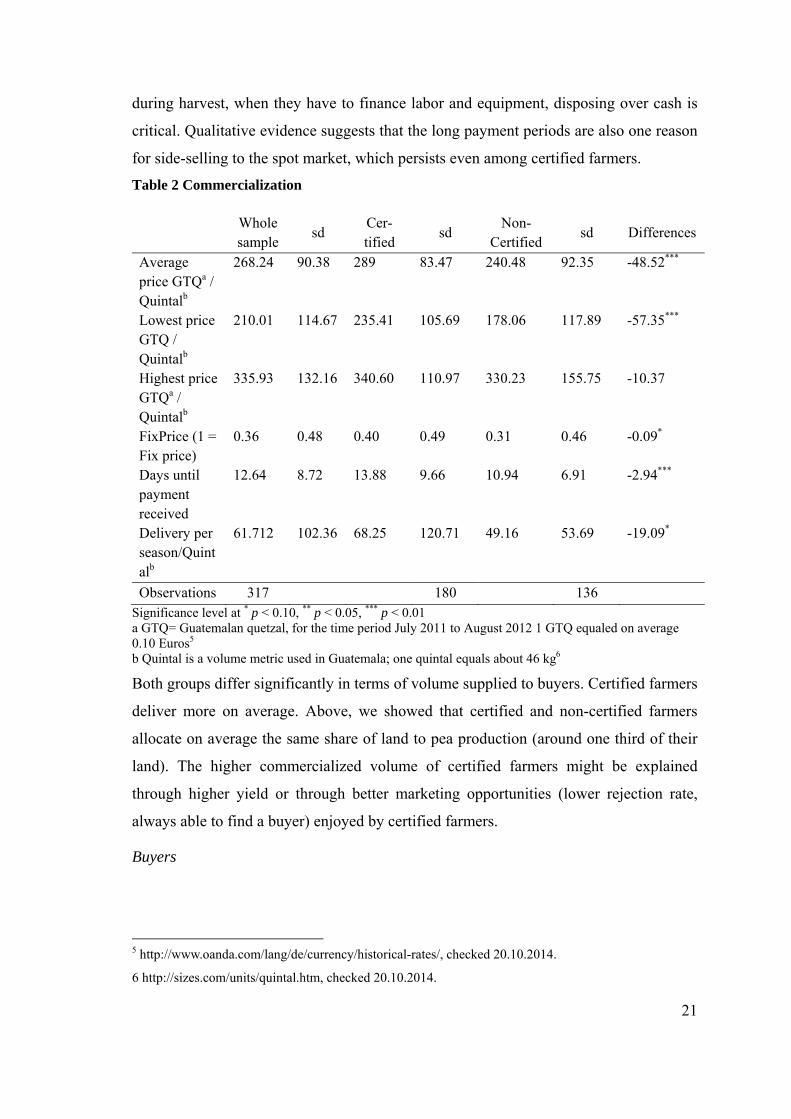
Commercialization
As we want to assess the economic impact of GlobalGAP adoption, we decided to first
acquire a descriptive overview of aspects of commercialization in the sample (see table
2). This will help us to understand under which conditions the farmers market their
products and how this might influence their economic situation. We asked the farmers
to report the average price they received for peas from their buyers during the reporting
time as well as the lowest and highest prices. In general, certified farmers receive a
higher average price than non-certified farmers. The lowest price received is
significantly lower for non-certified farmers than for certified farmers. Interestingly,
there is no statistically significant difference between the two groups when it comes to
the highest price received. According to the price information, it seems that certified
farmers experience fewer “price peaks” than non-certified farmers and receive more for
their product on average. GlobalGAP certification does not foresee a price premium for
compliance. To make certification more attractive for the farmers (and to avoid side-
selling), exporters offer certain price schemes. In our sample, 40% of the certified
farmers market their product under a fixed price scheme which represents a significant
difference to non-certified farmers. Fixed price schemes are not necessarily attached to
certification schemes. Even non-certified farmers supplying exporters engage in fixed
price schemes. Of course, fixed price schemes are not always good for the farmer. If the
market price is higher than the fixed price, there is room for arbitrage, and the farmer
could have earned more with the market price. This creates incentives for side-selling.
To avoid this, exporters often rely on a minimum price scheme, that is, they agree upon
a minimum price they always pay. If the market price is higher than the minimum price,
they pay the market price. We do not have information on minimum price schemes in
our sample.
Non-certified farmers have to wait significantly fewer days until they get paid than do
certified farmers. Farmers told us that the long waiting period for payment is one
disadvantage for them when it comes to supplying an exporter under a certification
scheme. Farmers in our sample have very few sources of cash income. Especially
21
during harvest, when they have to finance labor and equipment, disposing over cash is
critical. Qualitative evidence suggests that the long payment periods are also one reason
for side-selling to the spot market, which persists even among certified farmers.
Table 2 Commercialization
Significance level at * p < 0.10, ** p < 0.05, *** p < 0.01 a GTQ= Guatemalan quetzal, for the time period July 2011 to August 2012 1 GTQ equaled on average 0.10 Euros5 b Quintal is a volume metric used in Guatemala; one quintal equals about 46 kg6
Both groups differ significantly in terms of volume supplied to buyers. Certified farmers
deliver more on average. Above, we showed that certified and non-certified farmers
allocate on average the same share of land to pea production (around one third of their
land). The higher commercialized volume of certified farmers might be explained
through higher yield or through better marketing opportunities (lower rejection rate,
always able to find a buyer) enjoyed by certified farmers.
Buyers
5 http://www.oanda.com/lang/de/currency/historical-rates/, checked 20.10.2014.
6 http://sizes.com/units/quintal.htm, checked 20.10.2014.
Whole sample
sd Cer-tified
sd Non-
Certified sd Differences
Average price GTQa / Quintalb
268.24 90.38 289 83.47 240.48 92.35 -48.52***
Lowest price GTQ / Quintalb
210.01 114.67 235.41 105.69 178.06 117.89 -57.35***
Highest price GTQa / Quintalb
335.93 132.16 340.60 110.97 330.23 155.75 -10.37
FixPrice (1 = Fix price)
0.36 0.48 0.40 0.49 0.31 0.46 -0.09*
Days until payment received
12.64 8.72 13.88 9.66 10.94 6.91 -2.94***
Delivery per season/Quintalb
61.712 102.36 68.25 120.71 49.16 53.69 -19.09*
Observations 317 180 136
22
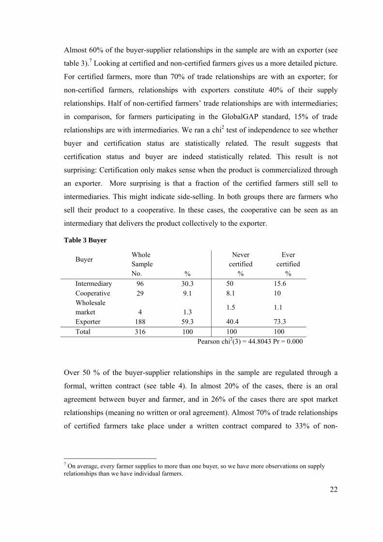
Almost 60% of the buyer-supplier relationships in the sample are with an exporter (see
table 3).7 Looking at certified and non-certified farmers gives us a more detailed picture.
For certified farmers, more than 70% of trade relationships are with an exporter; for
non-certified farmers, relationships with exporters constitute 40% of their supply
relationships. Half of non-certified farmers’ trade relationships are with intermediaries;
in comparison, for farmers participating in the GlobalGAP standard, 15% of trade
relationships are with intermediaries. We ran a chi2 test of independence to see whether
buyer and certification status are statistically related. The result suggests that
certification status and buyer are indeed statistically related. This result is not
surprising: Certification only makes sense when the product is commercialized through
an exporter. More surprising is that a fraction of the certified farmers still sell to
intermediaries. This might indicate side-selling. In both groups there are farmers who
sell their product to a cooperative. In these cases, the cooperative can be seen as an
intermediary that delivers the product collectively to the exporter.
Table 3 Buyer
Buyer Whole Sample
Never certified
Ever certified
No. % % %
Intermediary 96 30.3 50 15.6 Cooperative 29 9.1 8.1 10 Wholesale market 4 1.3
1.5 1.1
Exporter 188 59.3 40.4 73.3
Total 316 100 100 100
Pearson chi2(3) = 44.8043 Pr = 0.000
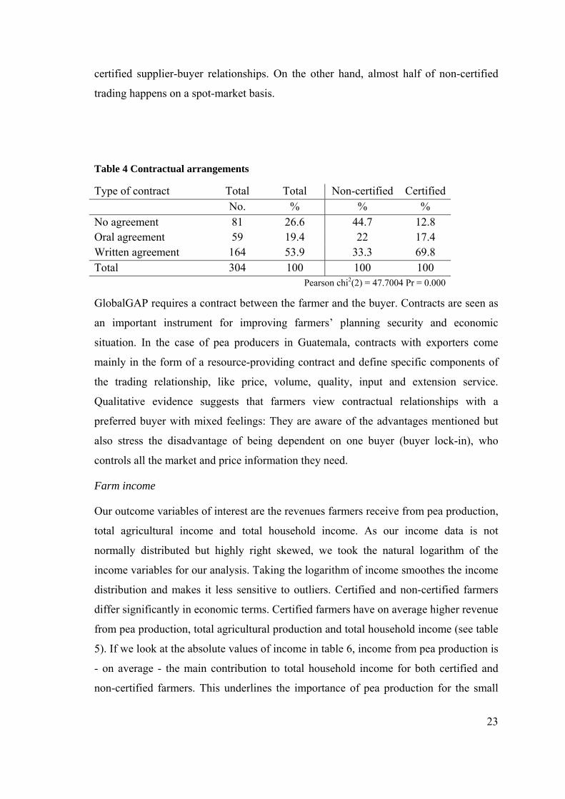
Over 50 % of the buyer-supplier relationships in the sample are regulated through a
formal, written contract (see table 4). In almost 20% of the cases, there is an oral
agreement between buyer and farmer, and in 26% of the cases there are spot market
relationships (meaning no written or oral agreement). Almost 70% of trade relationships
of certified farmers take place under a written contract compared to 33% of non-
7 On average, every farmer supplies to more than one buyer, so we have more observations on supply relationships than we have individual farmers.
23
certified supplier-buyer relationships. On the other hand, almost half of non-certified
trading happens on a spot-market basis.
Table 4 Contractual arrangements
Type of contract Total Total Non-certified Certified No. % % %
No agreement 81 26.6 44.7 12.8 Oral agreement 59 19.4 22 17.4 Written agreement 164 53.9 33.3 69.8 Total 304 100 100 100
Pearson chi2(2) = 47.7004 Pr = 0.000
GlobalGAP requires a contract between the farmer and the buyer. Contracts are seen as
an important instrument for improving farmers’ planning security and economic
situation. In the case of pea producers in Guatemala, contracts with exporters come
mainly in the form of a resource-providing contract and define specific components of
the trading relationship, like price, volume, quality, input and extension service.
Qualitative evidence suggests that farmers view contractual relationships with a
preferred buyer with mixed feelings: They are aware of the advantages mentioned but
also stress the disadvantage of being dependent on one buyer (buyer lock-in), who
controls all the market and price information they need.
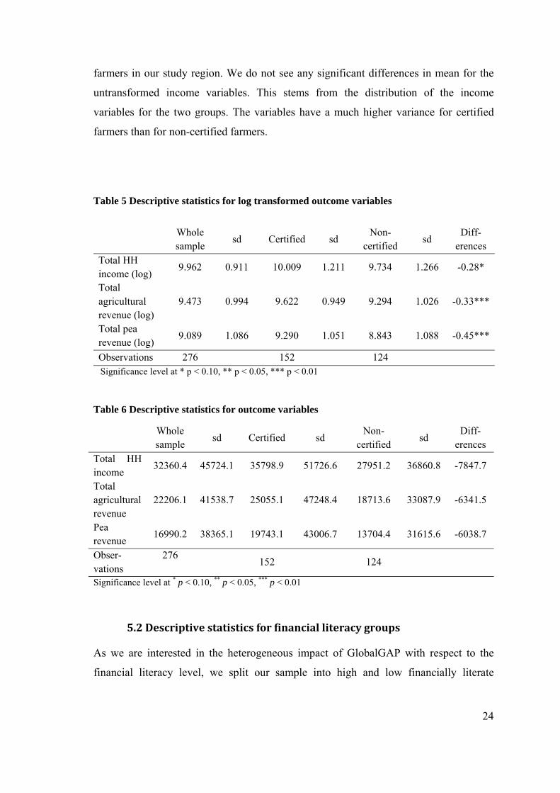
Farm income
Our outcome variables of interest are the revenues farmers receive from pea production,
total agricultural income and total household income. As our income data is not
normally distributed but highly right skewed, we took the natural logarithm of the
income variables for our analysis. Taking the logarithm of income smoothes the income
distribution and makes it less sensitive to outliers. Certified and non-certified farmers
differ significantly in economic terms. Certified farmers have on average higher revenue
from pea production, total agricultural production and total household income (see table
5). If we look at the absolute values of income in table 6, income from pea production is
- on average - the main contribution to total household income for both certified and
non-certified farmers. This underlines the importance of pea production for the small
24
farmers in our study region. We do not see any significant differences in mean for the
untransformed income variables. This stems from the distribution of the income
variables for the two groups. The variables have a much higher variance for certified
farmers than for non-certified farmers.
Table 5 Descriptive statistics for log transformed outcome variables
Table 6 Descriptive statistics for outcome variables
Whole sample
sd Certified sd Non-
certified sd
Diff-erences
Total HH income
32360.4 45724.1 35798.9 51726.6 27951.2 36860.8 -7847.7
Total agricultural revenue
22206.1 41538.7 25055.1 47248.4 18713.6 33087.9 -6341.5
Pea revenue
16990.2 38365.1 19743.1 43006.7 13704.4 31615.6 -6038.7
Obser-vations
276 152
124
Significance level at * p < 0.10, ** p < 0.05, *** p < 0.01
5.2Descriptivestatisticsforfinancialliteracygroups
As we are interested in the heterogeneous impact of GlobalGAP with respect to the
financial literacy level, we split our sample into high and low financially literate
Whole sample
sd Certified sd Non-
certified sd
Diff-erences
Total HH income (log)
9.962 0.911 10.009 1.211 9.734 1.266 -0.28*
Total agricultural revenue (log)
9.473 0.994 9.622 0.949 9.294 1.026 -0.33***
Total pea revenue (log)
9.089 1.086 9.290 1.051 8.843 1.088 -0.45***
Observations 276 152 124 Significance level at * p < 0.10, ** p < 0.05, *** p < 0.01
25
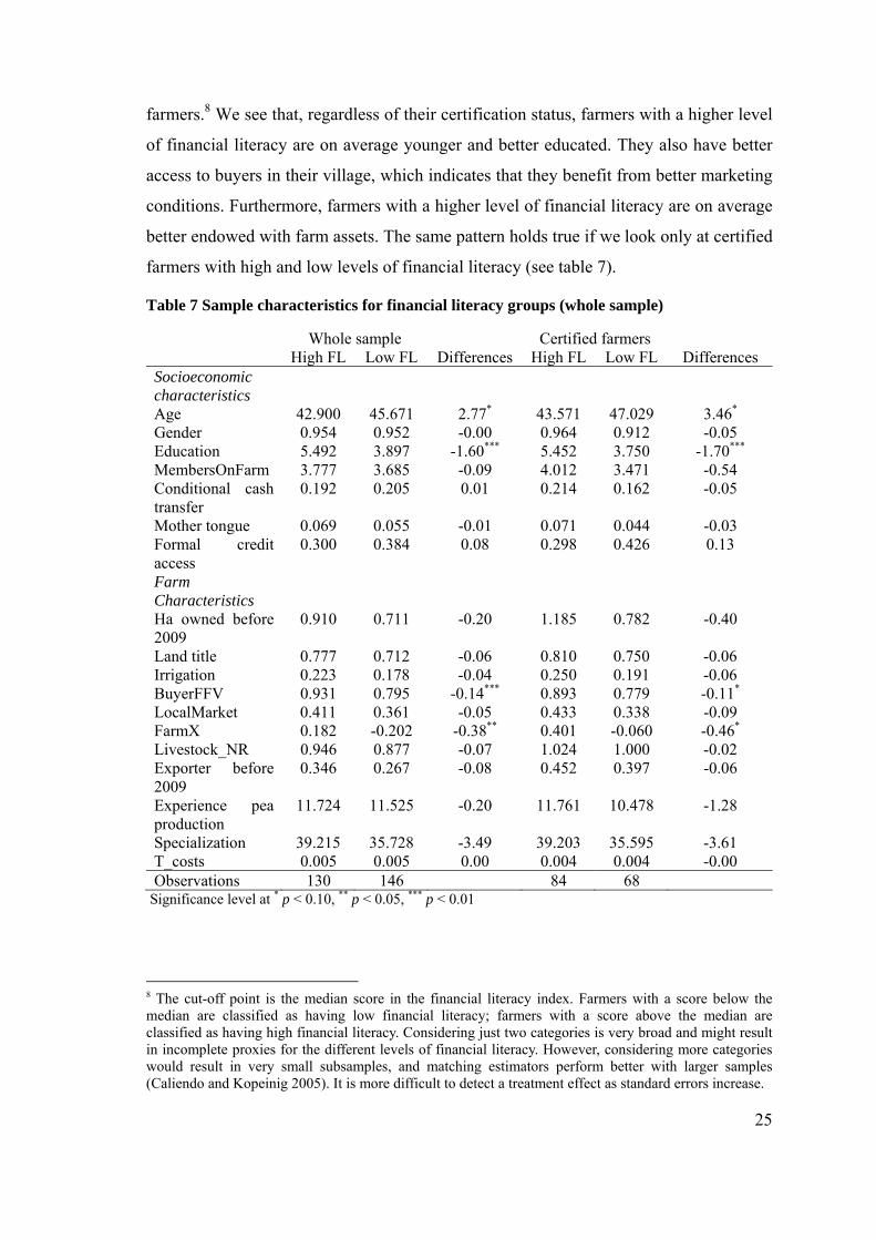
farmers.8 We see that, regardless of their certification status, farmers with a higher level
of financial literacy are on average younger and better educated. They also have better
access to buyers in their village, which indicates that they benefit from better marketing
conditions. Furthermore, farmers with a higher level of financial literacy are on average
better endowed with farm assets. The same pattern holds true if we look only at certified
farmers with high and low levels of financial literacy (see table 7).
Table 7 Sample characteristics for financial literacy groups (whole sample)
Whole sample Certified farmers High FL Low FL Differences High FL Low FL Differences Socioeconomic characteristics
Age 42.900 45.671 2.77* 43.571 47.029 3.46* Gender 0.954 0.952 -0.00 0.964 0.912 -0.05 Education 5.492 3.897 -1.60*** 5.452 3.750 -1.70*** MembersOnFarm 3.777 3.685 -0.09 4.012 3.471 -0.54 Conditional cash transfer
0.192 0.205 0.01 0.214 0.162 -0.05
Mother tongue 0.069 0.055 -0.01 0.071 0.044 -0.03 Formal credit access
0.300 0.384 0.08 0.298 0.426 0.13
Farm Characteristics
Ha owned before 2009
0.910 0.711 -0.20 1.185 0.782 -0.40
Land title 0.777 0.712 -0.06 0.810 0.750 -0.06 Irrigation 0.223 0.178 -0.04 0.250 0.191 -0.06 BuyerFFV 0.931 0.795 -0.14*** 0.893 0.779 -0.11* LocalMarket 0.411 0.361 -0.05 0.433 0.338 -0.09 FarmX 0.182 -0.202 -0.38** 0.401 -0.060 -0.46* Livestock_NR 0.946 0.877 -0.07 1.024 1.000 -0.02 Exporter before 2009
0.346 0.267 -0.08 0.452 0.397 -0.06
Experience pea production
11.724 11.525 -0.20 11.761 10.478 -1.28
Specialization 39.215 35.728 -3.49 39.203 35.595 -3.61 T_costs 0.005 0.005 0.00 0.004 0.004 -0.00 Observations 130 146 84 68
Significance level at * p < 0.10, ** p < 0.05, *** p < 0.01
8 The cut-off point is the median score in the financial literacy index. Farmers with a score below the median are classified as having low financial literacy; farmers with a score above the median are classified as having high financial literacy. Considering just two categories is very broad and might result in incomplete proxies for the different levels of financial literacy. However, considering more categories would result in very small subsamples, and matching estimators perform better with larger samples (Caliendo and Kopeinig 2005). It is more difficult to detect a treatment effect as standard errors increase.
26
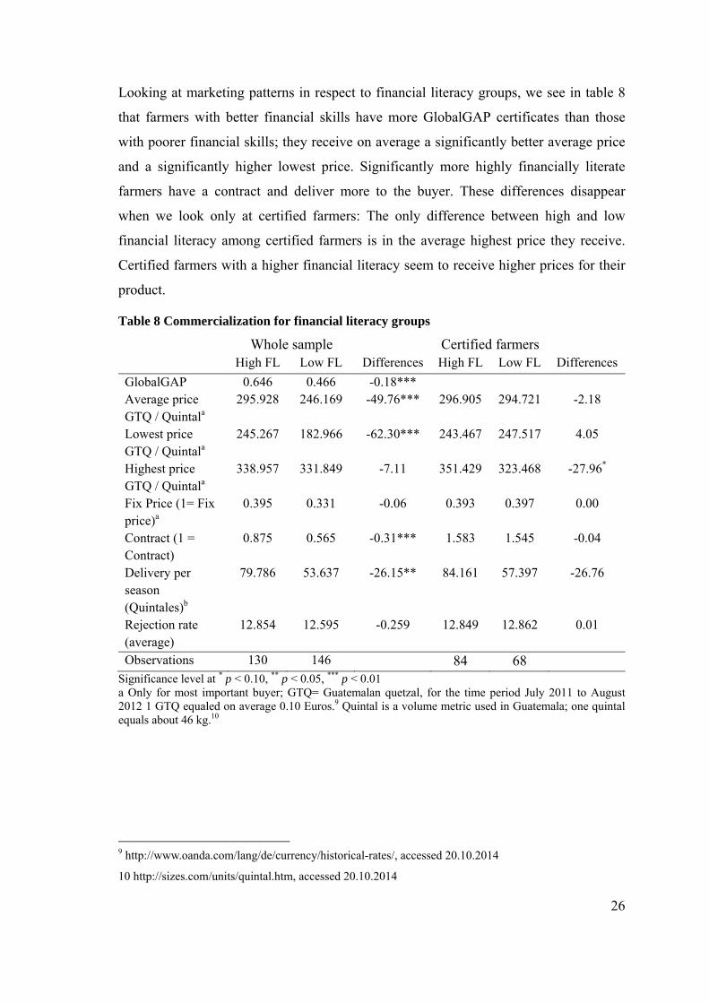
Looking at marketing patterns in respect to financial literacy groups, we see in table 8
that farmers with better financial skills have more GlobalGAP certificates than those
with poorer financial skills; they receive on average a significantly better average price
and a significantly higher lowest price. Significantly more highly financially literate
farmers have a contract and deliver more to the buyer. These differences disappear
when we look only at certified farmers: The only difference between high and low
financial literacy among certified farmers is in the average highest price they receive.
Certified farmers with a higher financial literacy seem to receive higher prices for their
product.
Table 8 Commercialization for financial literacy groups
Whole sample Certified farmers High FL Low FL Differences High FL Low FL Differences
GlobalGAP 0.646 0.466 -0.18*** Average price GTQ / Quintala
295.928 246.169 -49.76*** 296.905 294.721 -2.18
Lowest price GTQ / Quintala
245.267 182.966 -62.30*** 243.467 247.517 4.05
Highest price GTQ / Quintala
338.957 331.849 -7.11 351.429 323.468 -27.96*
Fix Price (1= Fix price)a
0.395 0.331 -0.06 0.393 0.397 0.00
Contract (1 = Contract)
0.875 0.565 -0.31*** 1.583 1.545 -0.04
Delivery per season (Quintales)b
79.786 53.637 -26.15** 84.161 57.397 -26.76
Rejection rate (average)
12.854 12.595 -0.259 12.849 12.862 0.01
Observations 130 146 84 68 Significance level at * p < 0.10, ** p < 0.05, *** p < 0.01 a Only for most important buyer; GTQ= Guatemalan quetzal, for the time period July 2011 to August 2012 1 GTQ equaled on average 0.10 Euros.9 Quintal is a volume metric used in Guatemala; one quintal equals about 46 kg.10
9 http://www.oanda.com/lang/de/currency/historical-rates/, accessed 20.10.2014
10 http://sizes.com/units/quintal.htm, accessed 20.10.2014
27
6. Propensity Score Matching Results
6.1TheimpactofGlobalGAPonfarmincome
Estimation of the Propensity Scores
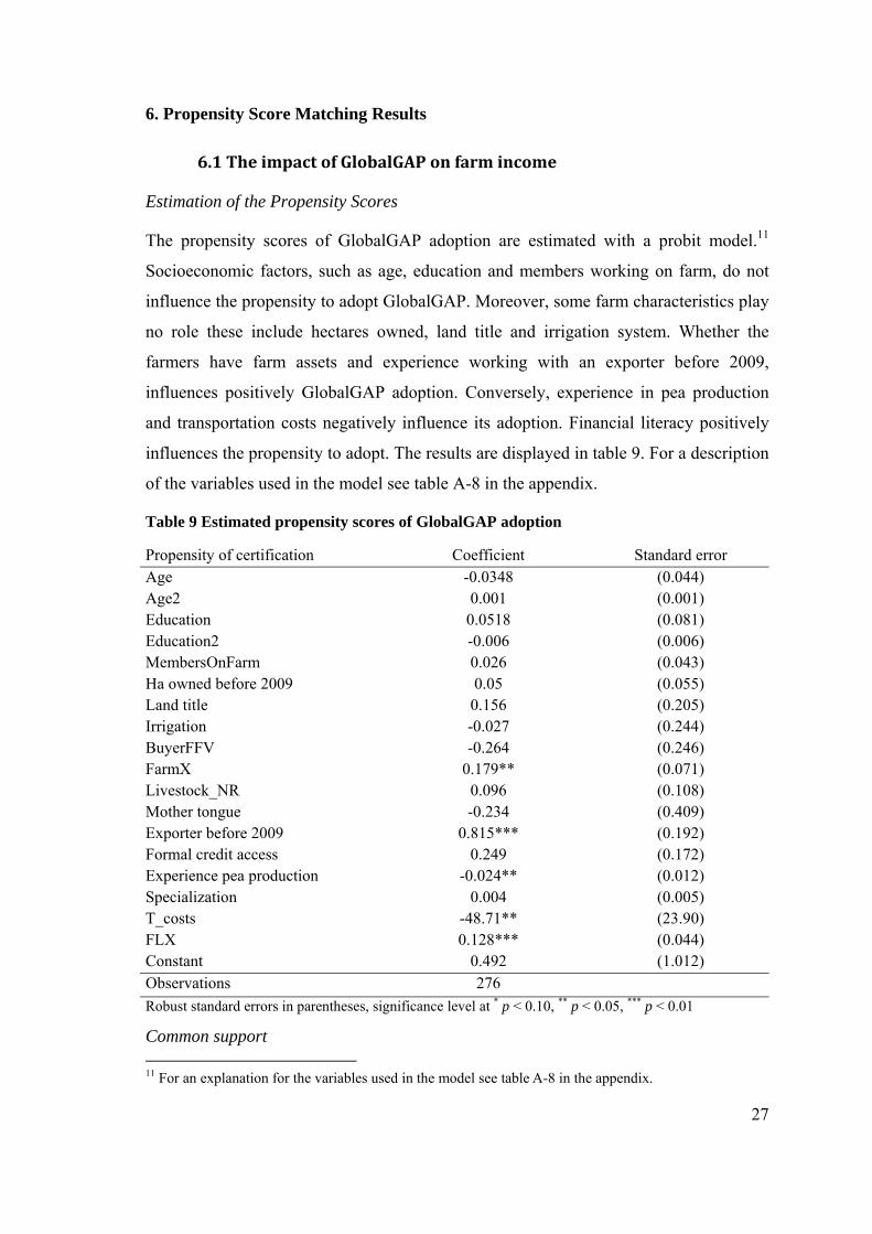
The propensity scores of GlobalGAP adoption are estimated with a probit model.11
Socioeconomic factors, such as age, education and members working on farm, do not
influence the propensity to adopt GlobalGAP. Moreover, some farm characteristics play
no role these include hectares owned, land title and irrigation system. Whether the
farmers have farm assets and experience working with an exporter before 2009,
influences positively GlobalGAP adoption. Conversely, experience in pea production
and transportation costs negatively influence its adoption. Financial literacy positively
influences the propensity to adopt. The results are displayed in table 9. For a description
of the variables used in the model see table A-8 in the appendix.
Table 9 Estimated propensity scores of GlobalGAP adoption
Propensity of certification Coefficient Standard errorAge -0.0348 (0.044) Age2 0.001 (0.001) Education 0.0518 (0.081) Education2 -0.006 (0.006) MembersOnFarm 0.026 (0.043) Ha owned before 2009 0.05 (0.055) Land title 0.156 (0.205) Irrigation -0.027 (0.244) BuyerFFV -0.264 (0.246) FarmX 0.179** (0.071) Livestock_NR 0.096 (0.108) Mother tongue -0.234 (0.409) Exporter before 2009 0.815*** (0.192) Formal credit access 0.249 (0.172) Experience pea production -0.024** (0.012) Specialization 0.004 (0.005) T_costs -48.71** (23.90) FLX 0.128*** (0.044) Constant 0.492 (1.012) Observations 276 Robust standard errors in parentheses, significance level at * p < 0.10, ** p < 0.05, *** p < 0.01
Common support 11 For an explanation for the variables used in the model see table A-8 in the appendix.
28
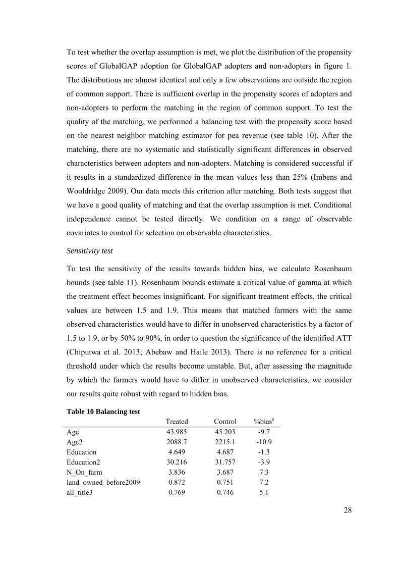
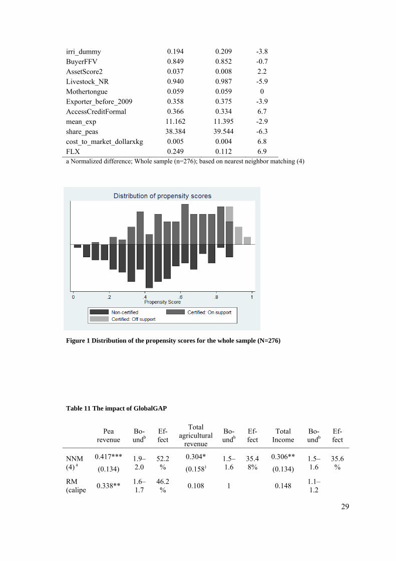
To test whether the overlap assumption is met, we plot the distribution of the propensity
scores of GlobalGAP adoption for GlobalGAP adopters and non-adopters in figure 1.
The distributions are almost identical and only a few observations are outside the region
of common support. There is sufficient overlap in the propensity scores of adopters and
non-adopters to perform the matching in the region of common support. To test the
quality of the matching, we performed a balancing test with the propensity score based
on the nearest neighbor matching estimator for pea revenue (see table 10). After the
matching, there are no systematic and statistically significant differences in observed
characteristics between adopters and non-adopters. Matching is considered successful if
it results in a standardized difference in the mean values less than 25% (Imbens and
Wooldridge 2009). Our data meets this criterion after matching. Both tests suggest that
we have a good quality of matching and that the overlap assumption is met. Conditional
independence cannot be tested directly. We condition on a range of observable
covariates to control for selection on observable characteristics.
Sensitivity test
To test the sensitivity of the results towards hidden bias, we calculate Rosenbaum
bounds (see table 11). Rosenbaum bounds estimate a critical value of gamma at which
the treatment effect becomes insignificant. For significant treatment effects, the critical
values are between 1.5 and 1.9. This means that matched farmers with the same
observed characteristics would have to differ in unobserved characteristics by a factor of
1.5 to 1.9, or by 50% to 90%, in order to question the significance of the identified ATT
(Chiputwa et al. 2013; Abebaw and Haile 2013). There is no reference for a critical
threshold under which the results become unstable. But, after assessing the magnitude
by which the farmers would have to differ in unobserved characteristics, we consider
our results quite robust with regard to hidden bias.
Table 10 Balancing test Treated Control %biasa
Age 43.985 45.203 -9.7
Age2 2088.7 2215.1 -10.9
Education 4.649 4.687 -1.3
Education2 30.216 31.757 -3.9
N_On_farm 3.836 3.687 7.3
land_owned_before2009 0.872 0.751 7.2
all_title3 0.769 0.746 5.1
29
irri_dummy 0.194 0.209 -3.8
BuyerFFV 0.849 0.852 -0.7
AssetScore2 0.037 0.008 2.2
Livestock_NR 0.940 0.987 -5.9
Mothertongue 0.059 0.059 0
Exporter_before_2009 0.358 0.375 -3.9
AccessCreditFormal 0.366 0.334 6.7
mean_exp 11.162 11.395 -2.9
share_peas 38.384 39.544 -6.3
cost_to_market_dollarxkg 0.005 0.004 6.8
FLX 0.249 0.112 6.9a Normalized difference; Whole sample (n=276); based on nearest neighbor matching (4)
Figure 1 Distribution of the propensity scores for the whole sample (N=276)
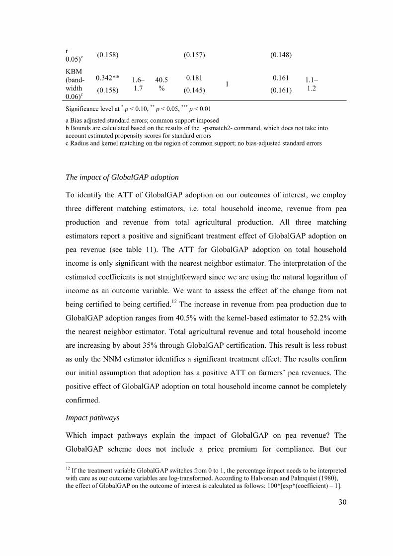
Table 11 The impact of GlobalGAP
Pea revenue
Bo-undb
Ef-fect
Total agricultural
revenue
Bo-undb
Ef-fect
Total Income
Bo-undb
Ef-fect
NNM (4) a
0.417***
(0.134)
1.9–2.0
52.2%
0.304*
(0.158)
1.5–1.6
35.48%
0.306**
(0.134)
1.5–1.6
35.6%
RM (calipe
0.338** 1.6–1.7
46.2%
0.108 1 0.148 1.1–1.2
30
r 0.05)c (0.158) (0.157) (0.148)
KBM (band-width 0.06)c
0.342**
(0.158)
1.6–1.7
40.5%
0.181
(0.145) 1
0.161
(0.161)
1.1–1.2
Significance level at * p < 0.10, ** p < 0.05, *** p < 0.01
a Bias adjusted standard errors; common support imposed b Bounds are calculated based on the results of the -psmatch2- command, which does not take into account estimated propensity scores for standard errors c Radius and kernel matching on the region of common support; no bias-adjusted standard errors
The impact of GlobalGAP adoption
To identify the ATT of GlobalGAP adoption on our outcomes of interest, we employ
three different matching estimators, i.e. total household income, revenue from pea
production and revenue from total agricultural production. All three matching
estimators report a positive and significant treatment effect of GlobalGAP adoption on
pea revenue (see table 11). The ATT for GlobalGAP adoption on total household
income is only significant with the nearest neighbor estimator. The interpretation of the
estimated coefficients is not straightforward since we are using the natural logarithm of
income as an outcome variable. We want to assess the effect of the change from not
being certified to being certified.12 The increase in revenue from pea production due to
GlobalGAP adoption ranges from 40.5% with the kernel-based estimator to 52.2% with
the nearest neighbor estimator. Total agricultural revenue and total household income
are increasing by about 35% through GlobalGAP certification. This result is less robust
as only the NNM estimator identifies a significant treatment effect. The results confirm
our initial assumption that adoption has a positive ATT on farmers’ pea revenues. The
positive effect of GlobalGAP adoption on total household income cannot be completely
confirmed.
Impact pathways
Which impact pathways explain the impact of GlobalGAP on pea revenue? The
GlobalGAP scheme does not include a price premium for compliance. But our
12 If the treatment variable GlobalGAP switches from 0 to 1, the percentage impact needs to be interpreted with care as our outcome variables are log-transformed. According to Halvorsen and Palmquist (1980), the effect of GlobalGAP on the outcome of interest is calculated as follows: 100*[exp*(coefficient) – 1].
31
descriptive results show that certified farmers benefit from a more beneficial pricing
scheme. Exporters offer premium prices and minimum or fixed price schemes in order
to make certification more attractive and avoid side-selling. Certified farmers benefit
from higher average prices, but prices do not fluctuate as much. The positive impact of
GlobalGAP on pea revenue might therefore result from a price effect. Still, we also see
that GlobalGAP producers generally deliver more to their exporters. On average, non-
certified farmers have smaller farms than certified farmers. But the farmers do not differ
in their specializations - both groups assign around 37% of their cultivated land to pea
production. The higher volume delivered may be due to higher absolute cultivation land
or to higher yields resulting from better production management, more efficient input
use and better extension service. Improvement in farmers’ marketing situation might
also explain the volume effect. First, GlobalGAP comes with a contract scheme. These
contracts often define the volume demanded by the exporter. Second, the improvement
in product quality through GlobalGAP may lead to a lower rejection rate. Hence, the
higher revenue from pea production for GlobalGAP certified farmers might also result
from a volume effect.
But why does the strong ATT on pea revenue not translate into an increase in total
agricultural revenue and total household income? Albeit the specialization in pea
production is the same for certified and non-certified farmers (see table 1), standard
adoption might require more capital and labor, which comes at the cost of producing
other crops (intensification vs. diversification of the production base). GlobalGAP
compliance is time and labor intensive; this might also come at the cost of lower
engagement in off-farm activities, for example. Around one-third of the certified farm
households do not report any off-farm income during the period surveyed. Qualitative
evidence from the field supports this impact pathway: Farmers state that they do not
necessarily feel a quantitative improvement in their overall economic situation, but that
they do benefit from more economic security and stability.
6.2TheimpactofGlobalGAPandfinancialliteracy
Other studies have shown the importance of considering the heterogeneity of farmers
when assessing the impact of standards/innovations on the economic situation of small
farmers (Holzapfel and Wollni 2014; Mendola 2007; Hansen and Trifković 2014). In
32
our study we consider heterogeneous financial literacy skills in the assessment of the
income effect of GlobalGAP adoption. We assume that the impact of GlobalGAP
depends on the individual farmer’s financial skills. Furthermore, higher financial
literacy might allow a farmer to better translate certification into economic benefits.
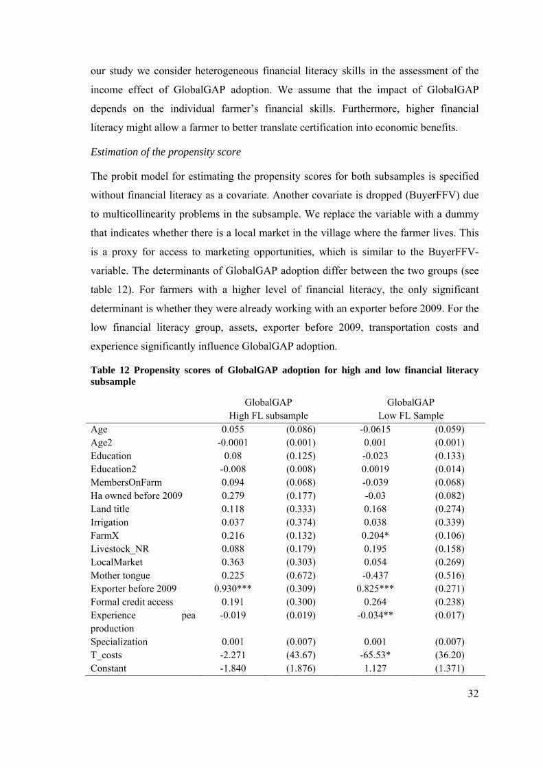
Estimation of the propensity score
The probit model for estimating the propensity scores for both subsamples is specified
without financial literacy as a covariate. Another covariate is dropped (BuyerFFV) due
to multicollinearity problems in the subsample. We replace the variable with a dummy
that indicates whether there is a local market in the village where the farmer lives. This
is a proxy for access to marketing opportunities, which is similar to the BuyerFFV-
variable. The determinants of GlobalGAP adoption differ between the two groups (see
table 12). For farmers with a higher level of financial literacy, the only significant
determinant is whether they were already working with an exporter before 2009. For the
low financial literacy group, assets, exporter before 2009, transportation costs and
experience significantly influence GlobalGAP adoption.
Table 12 Propensity scores of GlobalGAP adoption for high and low financial literacy subsample
GlobalGAP GlobalGAP High FL subsample Low FL Sample Age 0.055 (0.086) -0.0615 (0.059) Age2 -0.0001 (0.001) 0.001 (0.001) Education 0.08 (0.125) -0.023 (0.133) Education2 -0.008 (0.008) 0.0019 (0.014) MembersOnFarm 0.094 (0.068) -0.039 (0.068) Ha owned before 2009 0.279 (0.177) -0.03 (0.082) Land title 0.118 (0.333) 0.168 (0.274) Irrigation 0.037 (0.374) 0.038 (0.339) FarmX 0.216 (0.132) 0.204* (0.106) Livestock_NR 0.088 (0.179) 0.195 (0.158) LocalMarket 0.363 (0.303) 0.054 (0.269) Mother tongue 0.225 (0.672) -0.437 (0.516) Exporter before 2009 0.930*** (0.309) 0.825*** (0.271) Formal credit access 0.191 (0.300) 0.264 (0.238) Experience pea production
-0.019 (0.019) -0.034** (0.017)
Specialization 0.001 (0.007) 0.001 (0.007) T_costs -2.271 (43.67) -65.53* (36.20) Constant -1.840 (1.876) 1.127 (1.371)
33
Observations 130 146 Standard errors in parentheses * p<0.10, ** p<0.05, *** p<0.010
Common support
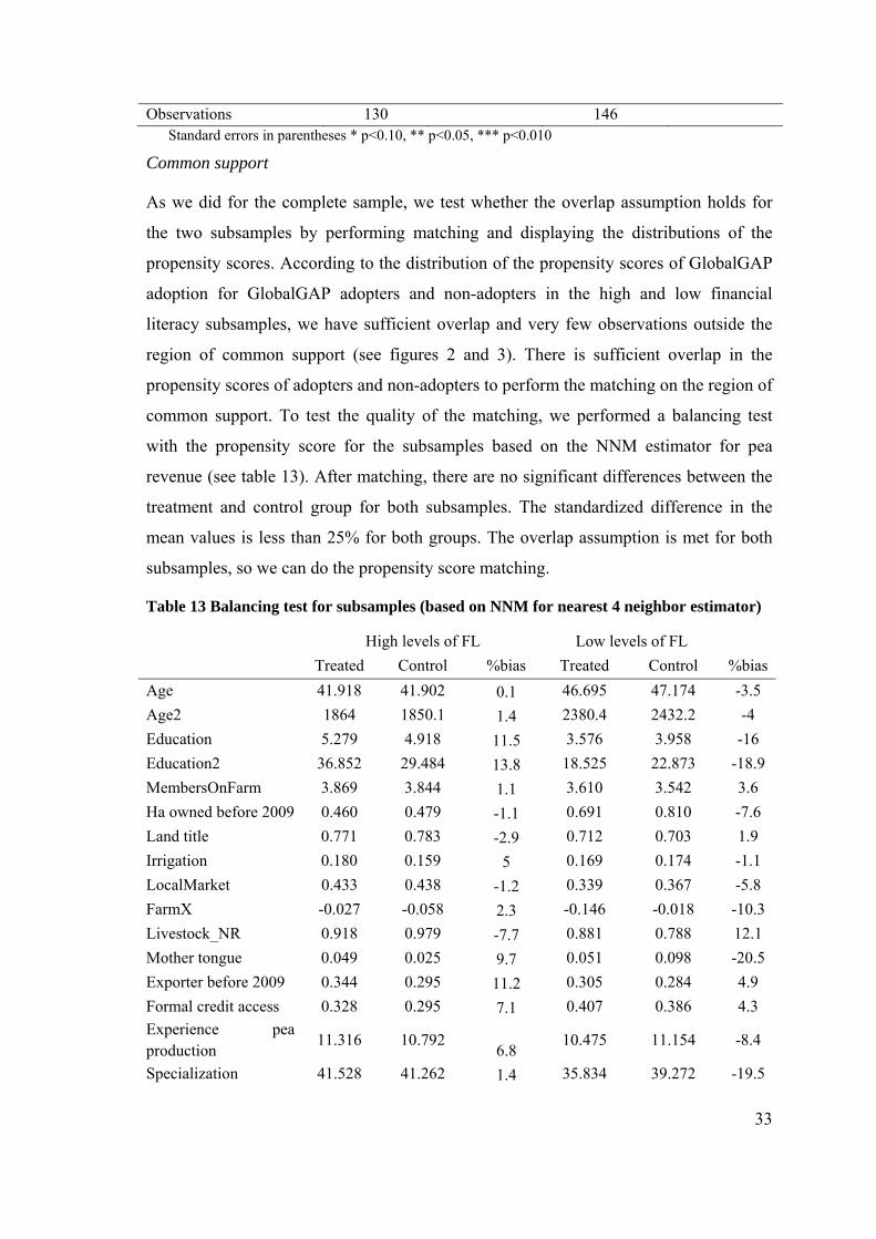
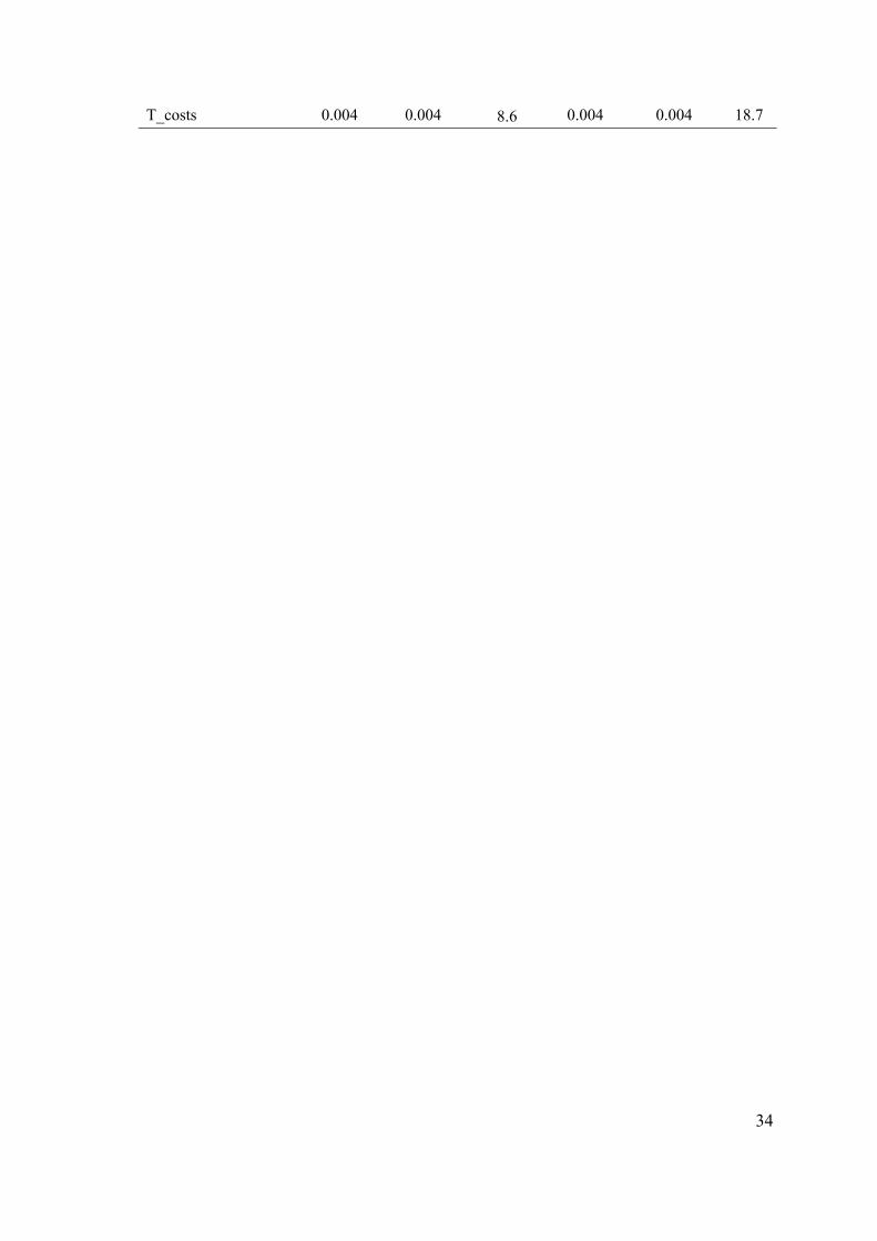
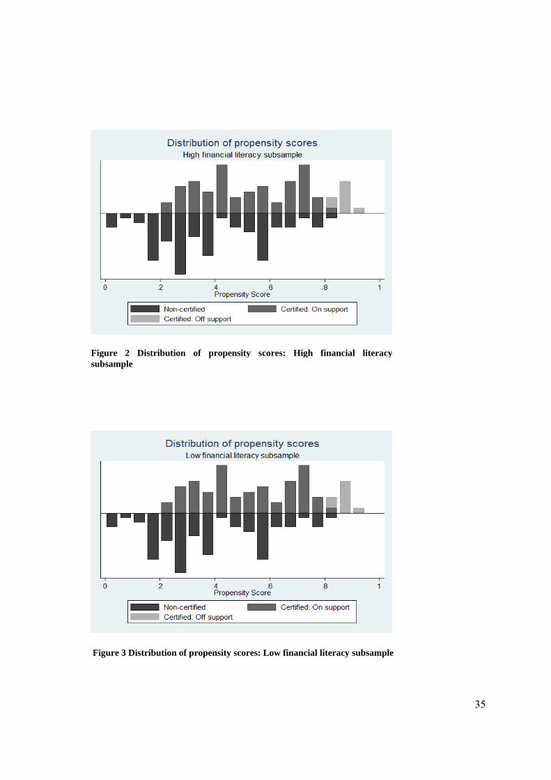
As we did for the complete sample, we test whether the overlap assumption holds for
the two subsamples by performing matching and displaying the distributions of the
propensity scores. According to the distribution of the propensity scores of GlobalGAP
adoption for GlobalGAP adopters and non-adopters in the high and low financial
literacy subsamples, we have sufficient overlap and very few observations outside the
region of common support (see figures 2 and 3). There is sufficient overlap in the
propensity scores of adopters and non-adopters to perform the matching on the region of
common support. To test the quality of the matching, we performed a balancing test
with the propensity score for the subsamples based on the NNM estimator for pea
revenue (see table 13). After matching, there are no significant differences between the
treatment and control group for both subsamples. The standardized difference in the
mean values is less than 25% for both groups. The overlap assumption is met for both
subsamples, so we can do the propensity score matching.
Table 13 Balancing test for subsamples (based on NNM for nearest 4 neighbor estimator)
High levels of FL Low levels of FL
Treated Control %bias Treated Control %bias
Age 41.918 41.902 0.1 46.695 47.174 -3.5
Age2 1864 1850.1 1.4 2380.4 2432.2 -4
Education 5.279 4.918 11.5 3.576 3.958 -16
Education2 36.852 29.484 13.8 18.525 22.873 -18.9
MembersOnFarm 3.869 3.844 1.1 3.610 3.542 3.6
Ha owned before 2009 0.460 0.479 -1.1 0.691 0.810 -7.6
Land title 0.771 0.783 -2.9 0.712 0.703 1.9
Irrigation 0.180 0.159 5 0.169 0.174 -1.1
LocalMarket 0.433 0.438 -1.2 0.339 0.367 -5.8
FarmX -0.027 -0.058 2.3 -0.146 -0.018 -10.3
Livestock_NR 0.918 0.979 -7.7 0.881 0.788 12.1
Mother tongue 0.049 0.025 9.7 0.051 0.098 -20.5
Exporter before 2009 0.344 0.295 11.2 0.305 0.284 4.9
Formal credit access 0.328 0.295 7.1 0.407 0.386 4.3
Experience pea production
11.316 10.792 6.8
10.475 11.154 -8.4
Specialization 41.528 41.262 1.4 35.834 39.272 -19.5
34
T_costs 0.004 0.004 8.6 0.004 0.004 18.7
35
Figure 2 Distribution of propensity scores: High financial literacysubsample
Figure 3 Distribution of propensity scores: Low financial literacy subsample
36
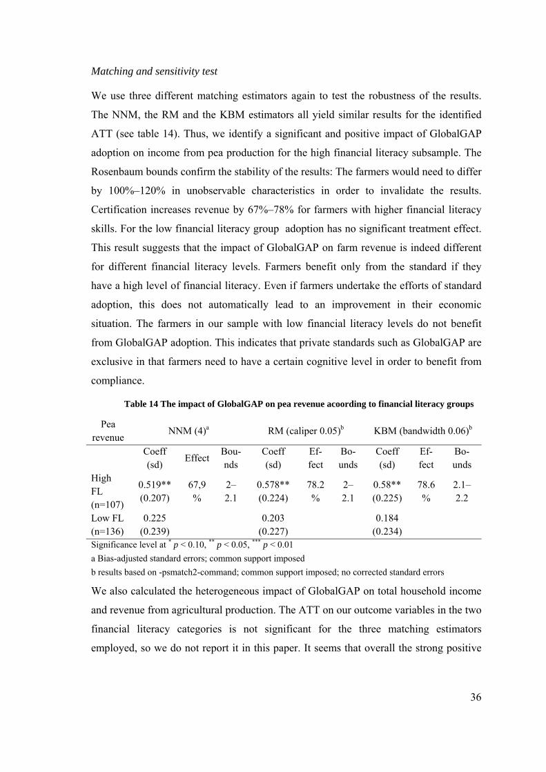
Matching and sensitivity test
We use three different matching estimators again to test the robustness of the results.
The NNM, the RM and the KBM estimators all yield similar results for the identified
ATT (see table 14). Thus, we identify a significant and positive impact of GlobalGAP
adoption on income from pea production for the high financial literacy subsample. The
Rosenbaum bounds confirm the stability of the results: The farmers would need to differ
by 100%–120% in unobservable characteristics in order to invalidate the results.
Certification increases revenue by 67%–78% for farmers with higher financial literacy
skills. For the low financial literacy group adoption has no significant treatment effect.
This result suggests that the impact of GlobalGAP on farm revenue is indeed different
for different financial literacy levels. Farmers benefit only from the standard if they
have a high level of financial literacy. Even if farmers undertake the efforts of standard
adoption, this does not automatically lead to an improvement in their economic
situation. The farmers in our sample with low financial literacy levels do not benefit
from GlobalGAP adoption. This indicates that private standards such as GlobalGAP are
exclusive in that farmers need to have a certain cognitive level in order to benefit from
compliance.
Table 14 The impact of GlobalGAP on pea revenue acoording to financial literacy groups
Pea revenue
NNM (4)a RM (caliper 0.05)b KBM (bandwidth 0.06)b
Coeff (sd)
Effect Bou-nds
Coeff (sd)
Ef-fect
Bo-unds
Coeff (sd)
Ef-fect
Bo-unds
High FL (n=107)
0.519** (0.207)
67,9%
2–2.1
0.578** (0.224)
78.2%
2–2.1
0.58** (0.225)
78.6%
2.1–2.2
Low FL (n=136)
0.225 (0.239)
0.203
(0.227)
0.184 (0.234)
Significance level at * p < 0.10, ** p < 0.05, *** p < 0.01
a Bias-adjusted standard errors; common support imposed
b results based on -psmatch2-command; common support imposed; no corrected standard errors
We also calculated the heterogeneous impact of GlobalGAP on total household income
and revenue from agricultural production. The ATT on our outcome variables in the two
financial literacy categories is not significant for the three matching estimators
employed, so we do not report it in this paper. It seems that overall the strong positive
37
effect of GlobalGAP on financially literate farmers does not translate into an overall
effect on total household income.13
Impact pathways
Financially literate farmers seem better able to translate GlobalGAP adoption into
economic benefits through their cognitive skills. But what can explain the strong and
heterogeneous impact of GlobalGAP on pea revenue? Referring to our conceptual
framework (outlined in section 2), financial literacy might influence the impact through
cognitive and non-cognitive effects.
The cognitive effect of financial literacy on farm income may work through different
channels. In the descriptive results, we saw that highly financially literate farmers are on
average better educated. Due to their higher educational and higher financial literacy
levels, they may be more used to applying numerical or financial concepts in their farm
management. This would help them in the efficient use of farm inputs, credits and
capital. They might also be more able to adequately use the information provided by the
standard, the standard setter and the extension environment. This would lead to better
management of the farm processes and closer compliance, which in turn might allow
farmers to produce more consistently high quality products. Better and more consistent
quality might lead to better prices. It may also be that exporters have to invest less into
the compliance of financially literate farmers and reward this with a higher price. As we
have seen in the descriptive results, on average farmers with higher scores on the
financial literacy index receive a better price, deliver more produce and have more
contracts compared to farmers with a low level of financial literacy. If we look at the
certified sample only, those with a higher financial literacy level receive the same
average price as farmers with a low financial literacy level, but they have higher price
ranges.
The non-cognitive effect of financial literacy may influence the income through
farmers` attitude and their bargaining ability. Highly financial literate farmers tend to be
younger, so they may be more open towards new technologies and more flexible in their
way of thinking. Another impact pathway of financial literacy on economic outcomes
may be through farmers’ bargaining ability. Having more accurate knowledge of the
13 Results upon request.
38
financial situation of their own farm businesses and understanding prices, interest and
inflation may improve farmers’ bargaining position. This may lead to higher prices for
their products.
Our descriptive results also show that those with a high financial literacy level have
easier access to marketing options for their product and work in an environment with
more competition among buyers. This might lead to better prices with the exporter.
Exporters might have an incentive to pay more or go with the market price to avoid
side-selling. Having a livelier commercial environment in the village may also offer
more learning opportunities for farmers, so that they can further improve their financial
abilities.
7. Conclusions
Smallholder farmers from developing countries are confronted with complex
regulations and requirements for their products and production processes. High quality,
safe and healthy food and sustainable production processes are demanded by consumers
around the world, mostly in developed countries. This demand translates into the
emergence of certification systems and standards, which have become more or less
mandatory and regulate access to international high-value chains. Increasing incomes
and the formation of a broader middle class in many developing countries and transition
economies fuel these trends. So far there is still no clear and undisputed answer as to
whether small farmers benefit from this trend. Empirical evidence suggests a positive
impact on the economic and household well-being of small farmers - but the impact is
not the same for all the farmers. We contribute to the discussion about the heterogeneity
of standards’ impacts by considering financial skills in measuring the economic impact
of a food safety and quality standard, GlobalGAP.
In this paper, we analyzed the impact of GlobalGAP adoption on the economic situation
of small pea farmers in the Guatemalan highlands. By using matching techniques we
showed the positive impact of GlobalGAP on revenue from pea production, total
agricultural revenue and the total household income of pea farmers in Guatemala.
Certified farmers benefit from beneficial price schemes and a more secure marketing
situation with binding agreements. The impact of GlobalGAP is heterogeneous
depending on the financial literacy level of the farmers: GlobalGAP has a strong and
39
significant positive effect on revenue from pea production for farmers with higher
financial literacy skills; for farmers with lower financial literacy skills, the impact
disappears. We do not detect any significant impact of GlobalGAP on total household
income when we stratify our sample into two groups based on financial literacy (high
and low). To check the sensitivity of our results towards hidden bias, we calculated
Rosenbaum bounds. The use of three different matching estimators confirms the
robustness of our results. Financial literacy seems to enable farmers to better translate
GlobalGAP adoption into economic benefits. Our results confirm our initial assumption
that the impact of food safety standards might be heterogeneous for differently skilled
farmers.
Our results hold important managerial and policy implications. Exporters are interested
in the continuous and reliable standard compliance of farmers. This allows exporters to
constantly deliver high quality, safe products to their buyers, who are mainly in Europe
or the US. Clear benefits from standard adoption are a strong incentive for farmers to
adhere to the standard. By improving farmers’ financial and other business-related skills
via extension services and trainings, benefits from organizational innovations such as
GlobalGAP could become more visible to those farmers. In this sense, this study of the
role of financial literacy has revealed an important starting point for increasing the
attractiveness of certification and farmers’ willingness to comply with standards.
Integration into high value chains is seen as a means to alleviate poverty and foster rural
development (FAO 2014). Public institutions and non-governmental organizations are,
therefore, increasingly interested in the implementation of public and private food safety
and quality standards in order to improve market integration of small farmers in
developing countries. Training farmers in financial and business-related skills could
help them benefit more from new technologies and decrease their vulnerability in the
competitive environment of global value chains. Standards might have positive
impulses for farm household well-being and rural development—as long as farmers
have the necessary skills to use new technologies for their own benefit. Thus, the study
also provides a starting point for political decisions and administrative actions aiming at
rural development and poverty alleviation.
Similar to most studies on the impact of the adoption of organizational innovations in
food supply chains, there are also some shortcomings. One important shortcoming of
40
the results is the potential endogeneity of GlobalGAP adoption. We control for this in
our analysis by matching on the area of common support, testing the balancing property
and calculating Rosenbaum bounds of hidden bias. This reduces bias in the results, but
does not completely eliminate it. Future research should take this problem into account.
Nevertheless we come to interesting results by exploring the role of financial literacy in
innovation adoption. It is important to consider farmers’ financial and other business-
related skills in order to better understand how new technologies like food safety and
quality standards impact farm level. Future research should deepen the understanding of
how cognitive skills influence the economic impact of new technologies. The ongoing
modernization and transformation of the global food system increasingly requires the
ability of farmers and other supply chain actors to adapt to a new business environment.
Ensuring the ability of farmers to make use of the opportunities provided to them by this
development is vital in creating benefits and improving resilience.

41
8. References
Abebaw, D.; Haile, M. G. (2013): The impact of cooperatives on agricultural
technology adoption: Empirical evidence from Ethiopia. In: Food Policy 38, 82–91.
Alene, Arega D.; Manyong, V. M. (2007): The effects of education on agricultural
productivity under traditional and improved technology in northern Nigeria: an
endogenous switching regression analysis. In: Empirical Economics 32 (1), 141–159.
Appleton, S.; Balihuta, A. (1996): Education and agricultural productivity: Evidence
from Uganda. In: Journal of International Development 8 (3), 415–444.
Asfaw, S.; Mithöfer, D.; Waibel, H. (2009): Investment in compliance with GlobalGAP
standards: does it pay off for small scale producers in Kenya? In: Quarterly Journal of
International Agriculture 48 (4), 337–362.
Atkinson, A.; Messy, F.-A. (2012): Measuring Financial Literacy: Results of the OECD
/ International Network on Financial Education (INEF) Pilot Study. OECD Working
Papers on Finance, Insurance and Private Pensions, No 15, OECD Publishing. Online:
http://dx.doi.org/10.1787/5k9csfs90fr4-en, accessed 5.12.2014.
Bandura, A. (1971): Social Learning Theory. New Cork City: General Learning Press.
Becker, S.; Caliendo, M. (2007): Sensitivity analysis for average treatment effects. In:
The Stata Journal 7 (1), 71–83.
Becker, S.; Ichino, A. (2002): Estimation of average treatment effects based on
propensity scores. In: The Stata Journal 2 (4), 358–377.
Behrmann, J.R; Mitchell, O.; Soo, C.; Bravo, D. (2010): Financial Literacy, Schooling
and Wealth Accumulation. National Bureau of Economic Research Working Paper
Series No. 16452. Online: http://www.nber.org/papers/w16452, accessed 26.06.2014.
42
Caliendo, M.; Kopeinig, S. (2005): Some Practical Guidance for the Implementation of
Propensity Score Matching. IZA Discussion Paper No. 1588.
Chiputwa, B.; Qaim, M.; Spielman, D. J. (2015): Food Standards, Certification and
Poverty among Coffee Farmers in Uganda. In: World Development 66, 400–412.
Cunguara, B.; Darnhofer, I. (2011): Assessing the impact of improved agricultural
technologies on household income in rural Mozambique. In: Food Policy 36 (3), 378–
390.
FAO (2014): Impact of international voluntary standards on smallholder market
participation in developing countries - A review of the literature. Food and Agriculture
Organization of the United Nations: Rome.
Gertler, P.; Martinez, S.; Premand, P.; Rawlings, L.; Vermeersch, C. (2011): Impact
Evaluation in Practice. The World Bank: Washington D.C. Online:
http://siteresources.worldbank.org/EXTHDOFFICE/Resources/5485726129545562862
0/Impact_Evaluation_in_Practice.pdf, accessed 5.12.2014.
GLOBALGAP (2013): Integrated Farm Assurance. Online:
http://www.GlobalGAP.org/
export/sites/default/.content/.galleries/documents/130315_gg_ifa_cpcc_af_cb_fv_v4_0-
2_en.pdf, accessed 19.11.2014.
Halvorsen, R.; Palmquist, R. (1980): The Interpretation of Dummy Variables in
Semilogarithmic Equations. In: The American Economic Review 70 (3), 474–475.
Handschuch, C.; Wollni, M.; Villalobos, P. (2013): Adoption of food safety and quality
standards among Chilean raspberry producers – Do smallholders benefit? In: Food
Policy 40, 64–73.
Hansen, H.; Trifković, N. (2014): Food Standards are Good – For Middle-Class
Farmers. In: World Development 56, 226–242.
Hanushek, E.; Woessmann, L. (2008): The Role of Cognitive Skills in Economic
Development. In: Journal of Economic Literature 46 (3), 607–668.
Henson, S.; Blandon J. (2007): The Impact of Food Safety Standards on Export-
Oriented Supply Chains: Case of the Horticultural Sector in Guatemala. Economic
Commission for Latin America and the Caribbean: Santiago de Chile. Online:
43
http://www.cepal.org/mexico/
capacidadescomerciales/TallerCRActH/Documentos/DOCTO_HENSON_FINAL.pdf,
accessed 12.11.2014.
Holzapfel, S.; Wollni, M. (2014): Is GlobalGAP Certification of Small-Scale Farmers
Sustainable? Evidence from Thailand. In: Journal of Development Studies 50 (5), 731–
747.
Imbens, G.; Wooldridge, J. (2009): Recent Developments in the Econometrics of
Program Evaluation. In: Journal of Economic Literature 47 (1), 5–86.
Jackson-Smith, D.; Trechter, D.; Splett, N. (2004): The Contribution of Financial
Management Training and Knowledge to Dairy Farm Financial Performance. In:
Review of Agricultural Economics 26 (1), 132–147.
Jamison, D.; Moock, P. (1984): Farmer Education and Farm Efficiency in Nepal: The
Role of Schooling, Extension Services, and Cognitive Skills. In: World Development 12
(1), 67–86.
Jolliffe, D. (1998): Skills, Schooling, and Household Income in Ghana. In: The World
Bank Economic Review 12 (1), 81–104.
Julian, J.; Sullivan, G.; Sánchez, G. (2000): Future Market Development Issues
Impacting Central America’s Nontraditional Agricultural Export Sector: Guatemala
Case Study. In: American Journal of Agricultural Economics 82 (5), 1177–1183.
Kieser, A. (1998): From Freemasons to Industrious Patriots: Organizing and
Disciplining in 18th Century Germany. In: Organization Studies 19 (1), 47–71.
Kolenikov, S.; Angeles, G. (2004): The Use of Discrete Data in PCA: Theory,
Simulations and Applications to Socioeconomic Indices. MEASURE Evaluation:
Chapel Hill. Online: http://www.cpc.unc.edu/measure/publications/wp-04-85, accessed
19.11.2014.
Langyintuo, A. S.; Mungoma, C. (2008): The effect of household wealth on the
adoption of improved maize varieties in Zambia. In: Food Policy 33 (6), 550–559.
Lockheed, M.; Jamison, T.; Lau, L. (1980): Farmer Education and Farm Efficiency: A
Survey. In: Economic Development and Cultural Change 29 (1), 37–76.
44
Lusardi, A.; Mitchell, O. S. (2014): The Economic Importance of Financial Literacy:
Theory and Evidence. In: Journal of Economic Literature 52 (1), 5–44.
Mendola, M. (2007): Agricultural technology adoption and poverty reduction: A
propensity-score matching analysis for rural Bangladesh. In: Food Policy 32 (3), 372–
393.
Müller, L.; Theuvsen, T. (2014): Food safety standards in the Guatemalan fresh pea
sector: The role of financial literacy in technology adoption. Unpublished work.
OECD INFE (2011): Measuring Financial Literacy: Questionnaire and Guidance Notes
for Conducting an Internationally Comparable Survey of Financial Literacy.
Organisation for Economic Co-operation and Development: Paris.
Rao, E.J.O; Qaim, M. (2011): Supermarkets, Farm Household Income, and Poverty:
Insights from Kenya. In: World Development 39 (5), 784–796.
Rusike, J.; Mahungu, N.M; Lukombo, S.S; Kendenga, T.; Bidiaka, S.M; Alene, A. et al.
(2014): Does a cassava research-for-development program have impact at the farm
level? Evidence from the Democratic Republic of Congo. In: Food Policy 46, 193–204.
Subervie, J.; Vagneron, I. (2013): A Drop of Water in the Indian Ocean? The Impact of
GlobalGAP Certification on Lychee Farmers in Madagascar. In: World Development
50, 57–73.
Vyas, S.; Kumaranayake, L. (2006): Constructing socio-economic status indices: how to
use principal components analysis. In: Health Policy and Planning 21 (6), 459–468.
Willems, S.; Roth, E.; van Roekel, J. (2005): Changing European Public and Private
Food Safety and Quality Requirements: Challenges for Developing Countries Fresh
Produce and Fish Exporters. The World Bank, Washington, D.C. Online:
http://siteresources.worldbank.org/INTARD/Resources/EU_Paper_final.pdf, accessed
5.12.2014.
45
9. Appendix
A1 Numeracy and financial literacy test
If there is a possibility of 10% of getting ill, how many persons out of 100 would get ill?
Five persons have bought the winning number in a lottery. The prize is 2,000 quetzals.
How much will each winner receive?
Imagine you had 1,000 quetzals in a savings account. The annual interest rate is 2% (20
quetzals in the first year). After five years, how much will you have in the saving
account if you do not touch the money?
More than 1020 quetzals
Exactly 1020 quetzals
Less than 1020 quetzals
Imagine that your income will double next year. The prices of all the products that you
consume will also double. With your income, how much will you be able to buy next
year?
More than this year
The same as this year
Less that this year
The bank has leant you 3,000 quetzals; the interest rate is 1% every month. If you pay
30 quetzals every month, when will you have paid back the loan?
In less than five years
In less than ten years
Never
Imagine you get a loan of 1,000 quetzals from the bank. Which option is better for you?
To pay 5% interest every month
To pay 24% interest a year
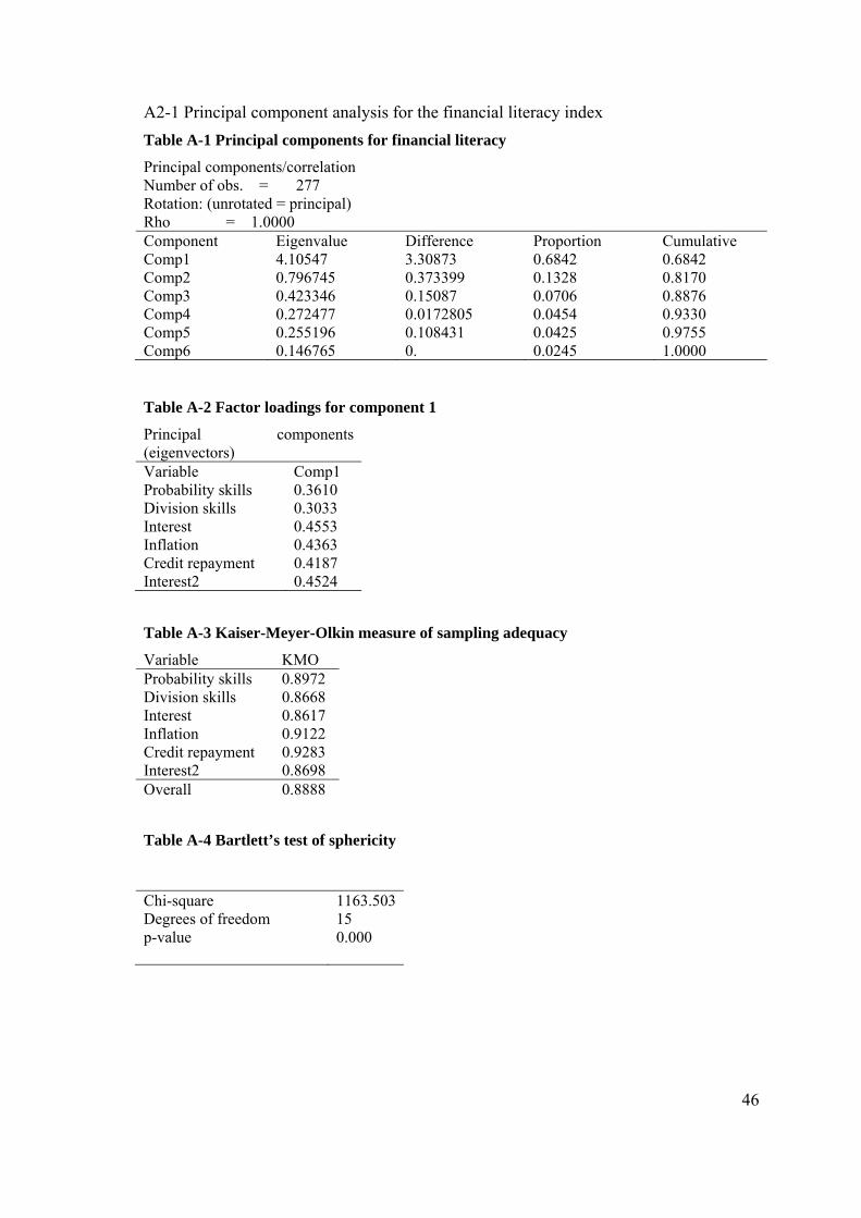
46
A2-1 Principal component analysis for the financial literacy index
Table A-1 Principal components for financial literacy
Principal components/correlation Number of obs. = 277 Rotation: (unrotated = principal) Rho = 1.0000 Component Eigenvalue Difference Proportion Cumulative Comp1 4.10547 3.30873 0.6842 0.6842 Comp2 0.796745 0.373399 0.1328 0.8170 Comp3 0.423346 0.15087 0.0706 0.8876 Comp4 0.272477 0.0172805 0.0454 0.9330 Comp5 0.255196 0.108431 0.0425 0.9755 Comp6 0.146765 0. 0.0245 1.0000
Table A-2 Factor loadings for component 1
Principal components (eigenvectors) Variable Comp1 Probability skills 0.3610 Division skills 0.3033 Interest 0.4553 Inflation 0.4363 Credit repayment 0.4187 Interest2 0.4524
Table A-3 Kaiser-Meyer-Olkin measure of sampling adequacy
Variable KMO Probability skills 0.8972 Division skills 0.8668 Interest 0.8617 Inflation 0.9122 Credit repayment 0.9283 Interest2 0.8698 Overall 0.8888
Table A-4 Bartlett’s test of sphericity
Chi-square 1163.503Degrees of freedom 15 p-value 0.000
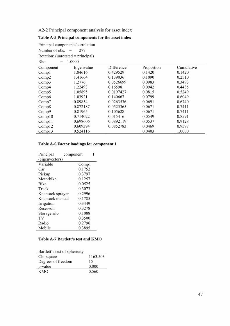
47
A2-2 Principal component analysis for asset index
Table A-5 Principal components for the asset index
Table A-6 Factor loadings for component 1
Table A-7 Bartlett’s test and KMO
Principal components/correlation Number of obs. = 277 Rotation: (unrotated = principal) Rho = 1.0000 Component Eigenvalue Difference Proportion Cumulative Comp1 1.84616 0.429529 0.1420 0.1420 Comp2 1.41664 0.139036 0.1090 0.2510 Comp3 1.2776 0.0526699 0.0983 0.3493 Comp4 1.22493 0.16598 0.0942 0.4435 Comp5 1.05895 0.0197427 0.0815 0.5249 Comp6 1.03921 0.140667 0.0799 0.6049 Comp7 0.89854 0.0263536 0.0691 0.6740 Comp8 0.872187 0.0525365 0.0671 0.7411 Comp9 0.81965 0.105628 0.0671 0.7411 Comp10 0.714022 0.015416 0.0549 0.8591 Comp11 0.698606 0.0892119 0.0537 0.9128 Comp12 0.609394 0.0852783 0.0469 0.9597 Comp13 0.524116 0.0403 1.0000
Principal component 1 (eigenvectors) Variable Comp1 Car 0.1752 Pickup 0.3797 Motorbike 0.1257 Bike 0.0525 Truck 0.3073 Knapsack sprayer 0.2996 Knapsack manual 0.1785 Irrigation 0.3449 Reservoir 0.3278 Storage silo 0.1088 TV 0.3500 Radio 0.2796 Mobile 0.3895
Bartlett’s test of sphericity Chi-square 1163.503Degrees of freedom 15 p-value 0.000 KMO 0.560
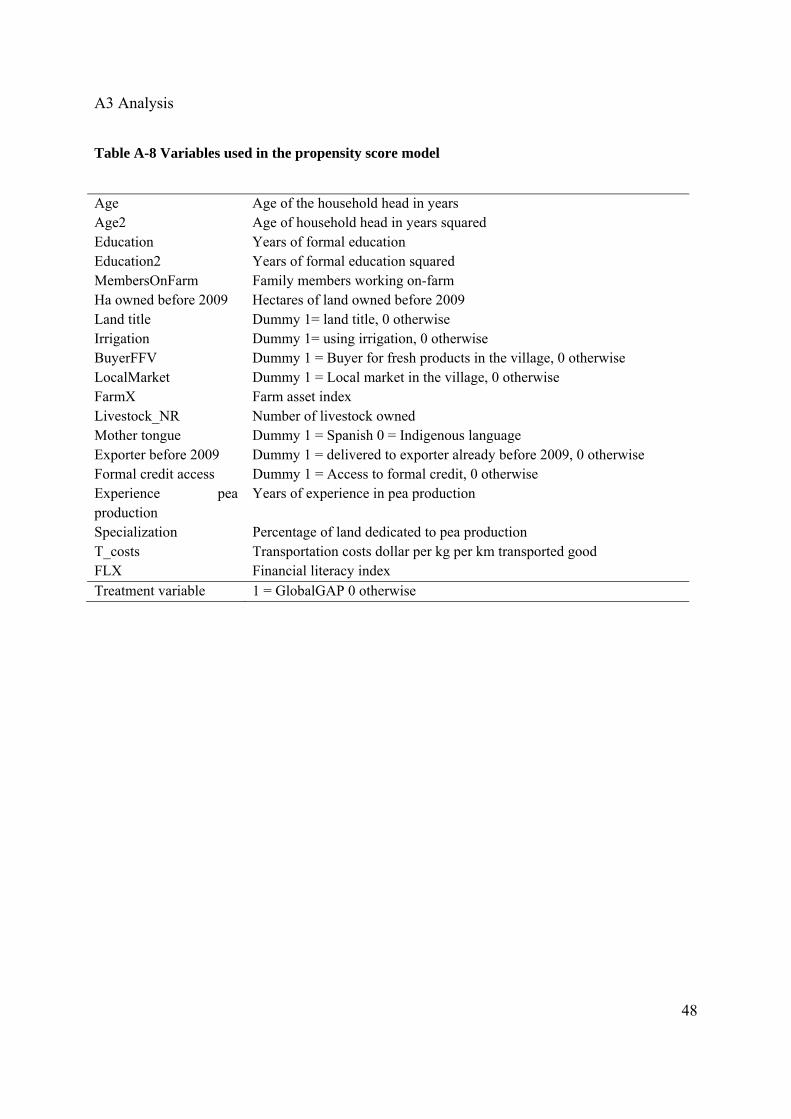
48
A3 Analysis
Table A-8 Variables used in the propensity score model
Age Age of the household head in years Age2 Age of household head in years squared Education Years of formal education Education2 Years of formal education squared MembersOnFarm Family members working on-farm Ha owned before 2009 Hectares of land owned before 2009 Land title Dummy 1= land title, 0 otherwise Irrigation Dummy 1= using irrigation, 0 otherwise BuyerFFV Dummy 1 = Buyer for fresh products in the village, 0 otherwise LocalMarket Dummy 1 = Local market in the village, 0 otherwise FarmX Farm asset index Livestock_NR Number of livestock owned Mother tongue Dummy 1 = Spanish 0 = Indigenous language Exporter before 2009 Dummy 1 = delivered to exporter already before 2009, 0 otherwise Formal credit access Dummy 1 = Access to formal credit, 0 otherwise Experience pea production
Years of experience in pea production
Specialization Percentage of land dedicated to pea production T_costs Transportation costs dollar per kg per km transported good FLX Financial literacy index Treatment variable 1 = GlobalGAP 0 otherwise