Sampling and Reconstruction - cs.utexas.eduSampling and Reconstruction. University of Texas at Austin CS384G - Computer Graphics Spring 2010 Don Fussell 2 Reading ... What is an image?

University of Texas at Austin CS384G - Computer Graphics Spring 2010 Don Fussell

Sampling and Reconstruction

University of Texas at Austin CS384G - Computer Graphics Spring 2010 Don Fussell 2

Reading

Required:Watt, Section 14.1

Recommended:Ron Bracewell, The Fourier Transform and ItsApplications, McGraw-Hill.Don P. Mitchell and Arun N. Netravali,“Reconstruction Filters in Computer ComputerGraphics ,” Computer Graphics, (Proceedingsof SIGGRAPH 88). 22 (4), pp. 221-228, 1988.


What is an image?

We can think of an image as a function, f, from R2 to R:f( x, y ) gives the intensity of a channel at position ( x, y )Realistically, we expect the image only to be defined over arectangle, with a finite range:

f: [a,b]x[c,d] [0,1]

A color image is just three functions pasted together. Wecan write this as a “vector-valued” function:

We’ll focus in grayscale (scalar-valued) images for now.

( , )

( , ) ( , )

( , )

r x y

f x y g x y

b x y

! "# $

= # $# $% &


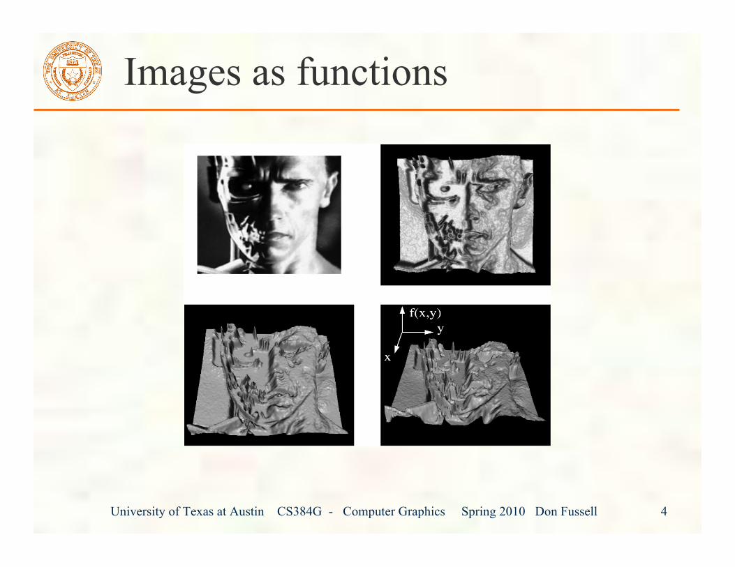
Images as functions


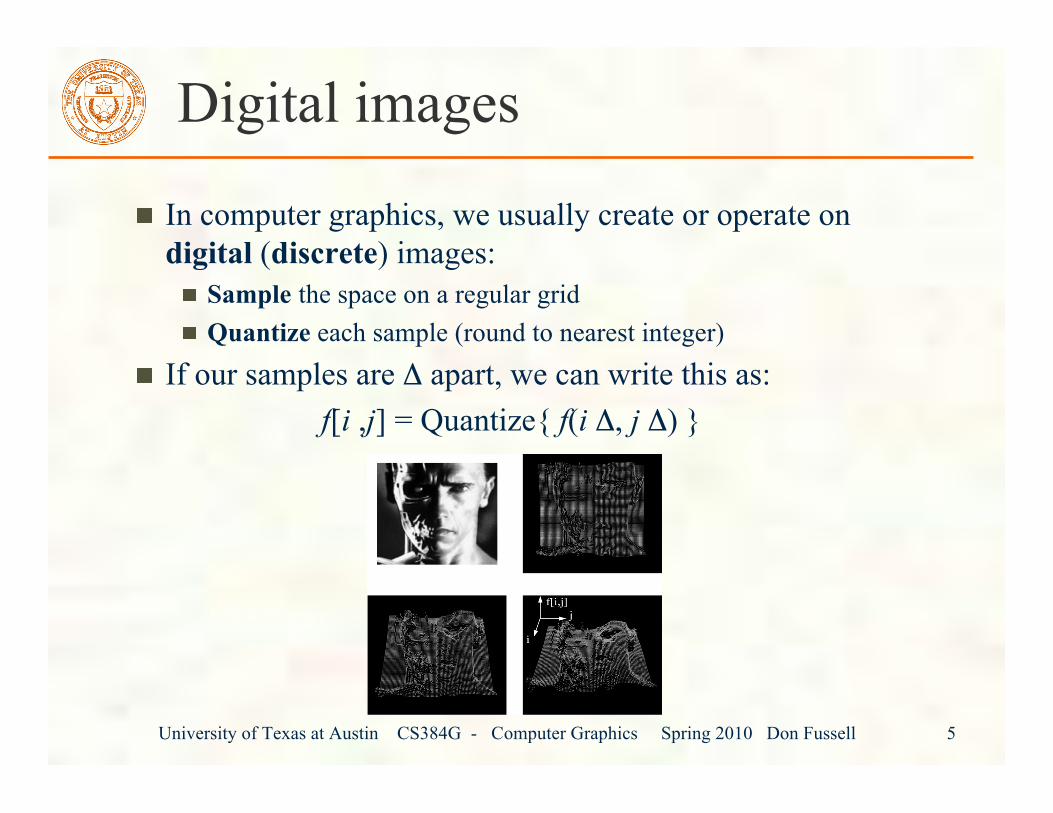
Digital images

In computer graphics, we usually create or operate ondigital (discrete) images:

Sample the space on a regular gridQuantize each sample (round to nearest integer)

If our samples are Δ apart, we can write this as:f[i ,j] = Quantize{ f(i Δ, j Δ) }


Motivation: filtering and resizing

What if we now want to:smooth an image?sharpen an image?enlarge an image?shrink an image?

Before we try these operations, it’s helpfulto think about images in a moremathematical way…


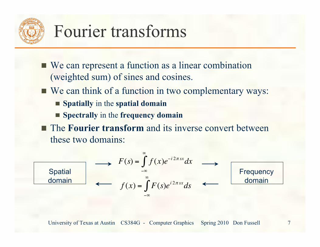
Fourier transforms

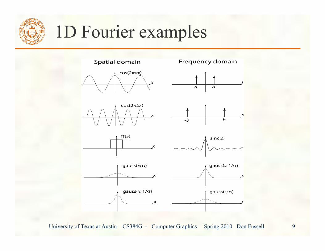
We can represent a function as a linear combination(weighted sum) of sines and cosines.We can think of a function in two complementary ways:

Spatially in the spatial domainSpectrally in the frequency domain

The Fourier transform and its inverse convert betweenthese two domains:

Frequencydomain

Spatialdomain

!

F(s) = f (x)e" i 2# sx

"$

$

% dx

!

f (x) = F(s)ei 2" sx

#$

$

% ds


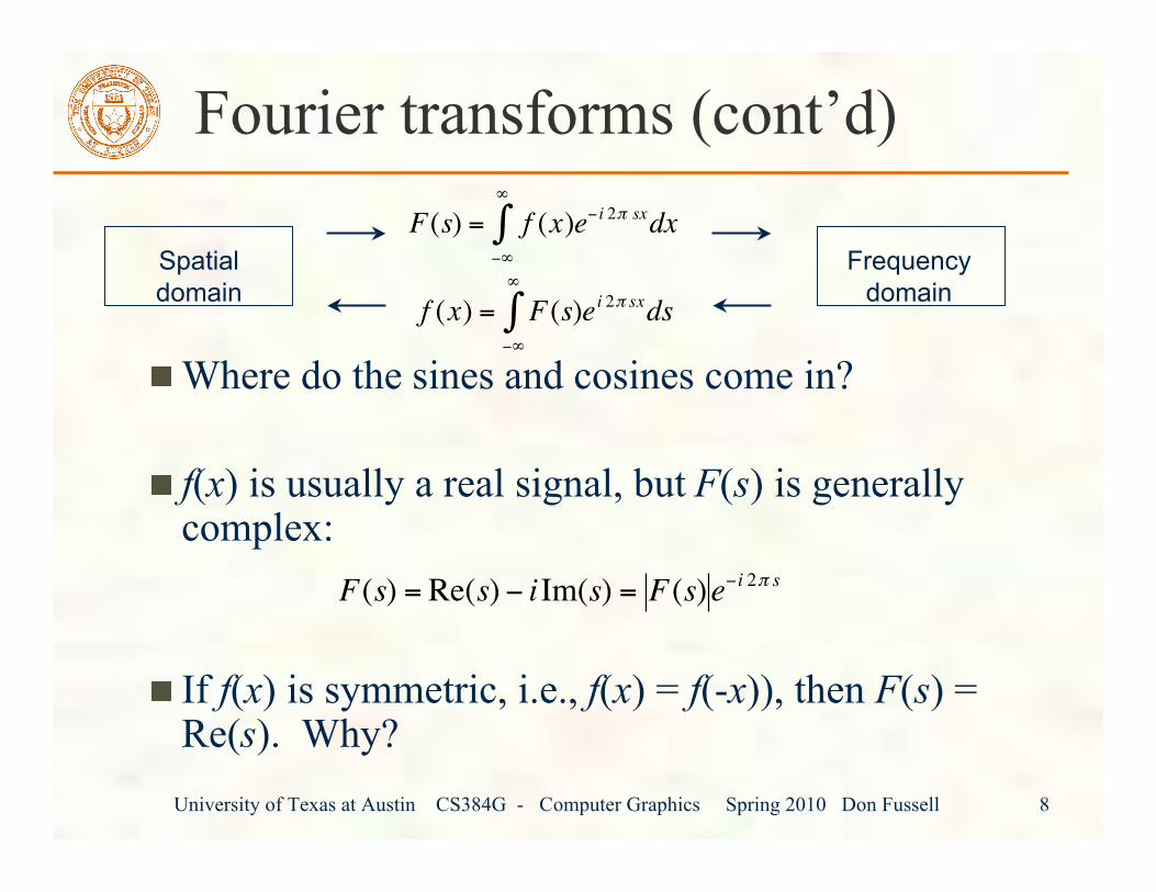
Fourier transforms (cont’d)

Where do the sines and cosines come in?

f(x) is usually a real signal, but F(s) is generallycomplex:

If f(x) is symmetric, i.e., f(x) = f(-x)), then F(s) =Re(s). Why?

Frequencydomain

Spatialdomain

!

F(s) = f (x)e" i 2# sx

"$

$

% dx

!

f (x) = F(s)ei 2" sx

#$

$

% ds

!

F(s) = Re(s) " iIm(s) = F(s)e"i 2# s


1D Fourier examples


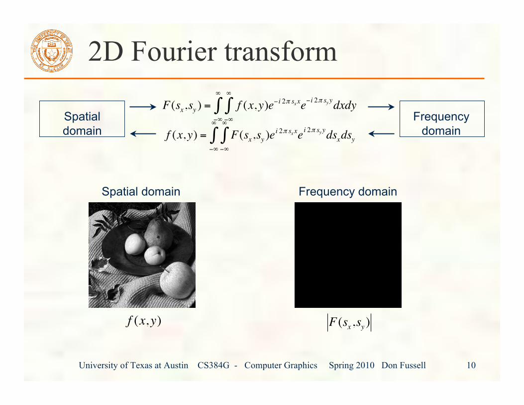
2D Fourier transform

Frequencydomain

Spatialdomain

Spatial domain Frequency domain

!

F(sx,sy ) = f (x,y)e" i 2# sxx

"$

$

%"$

$

% e"i 2# syydxdy

!

f (x,y) = F(sx,sy )ei 2" sxx

#$

$

%#$

$

% ei 2" syydsxdsy

!

f (x,y)

!

F(sx,sy )


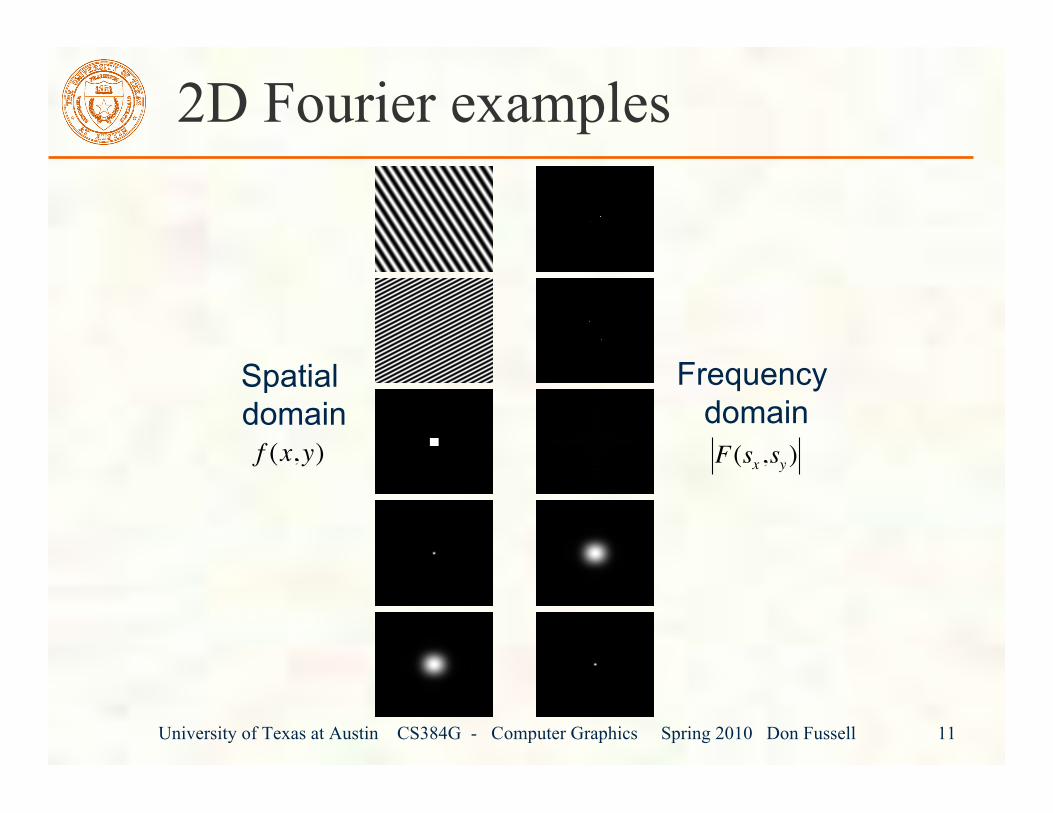
2D Fourier examples

Spatial domain

Frequency domain

!

f (x,y)

!

F(sx,sy )


Convolution

One of the most common methods for filtering afunction is called convolution.In 1D, convolution is defined as:

where

!

) h (x) = h("x)

!

g(x) = f (x) * h(x)

= f ( " x )h(x # " x )d " x #$

$

%

= f ( " x )) h ( " x # x)d " x

#$

$

%


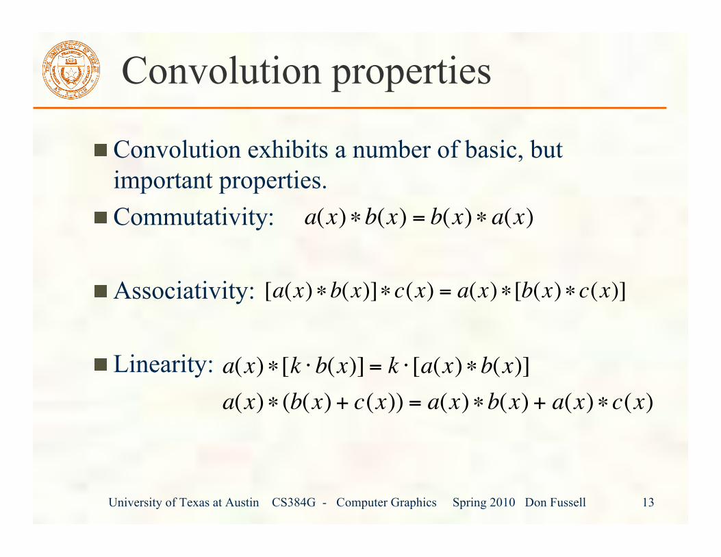
Convolution properties

Convolution exhibits a number of basic, butimportant properties.Commutativity:

Associativity:

Linearity:

!

a(x)"b(x) = b(x)" a(x)

!

[a(x)"b(x)]"c(x) = a(x)"[b(x)"c(x)]

!

a(x)"[k # b(x)] = k # [a(x)"b(x)]

a(x)" (b(x) + c(x)) = a(x)"b(x) + a(x)"c(x)


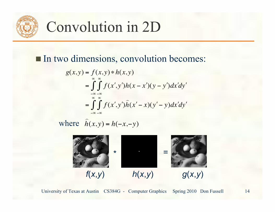
Convolution in 2D

In two dimensions, convolution becomes:

where

* =

f(x,y) h(x,y) g(x,y)

!

) h (x,y) = h("x,"y)

!

g(x,y) = f (x,y)" h(x,y)

= f ( # x , # y )h(x $ # x )(y $ # y )d # x d # y $%

%

&$%

%

&

= f ( # x , # y )) h ( # x $ x)( # y $ y)d # x d # y

$%

%

&$%

%

&


Convolution theorems

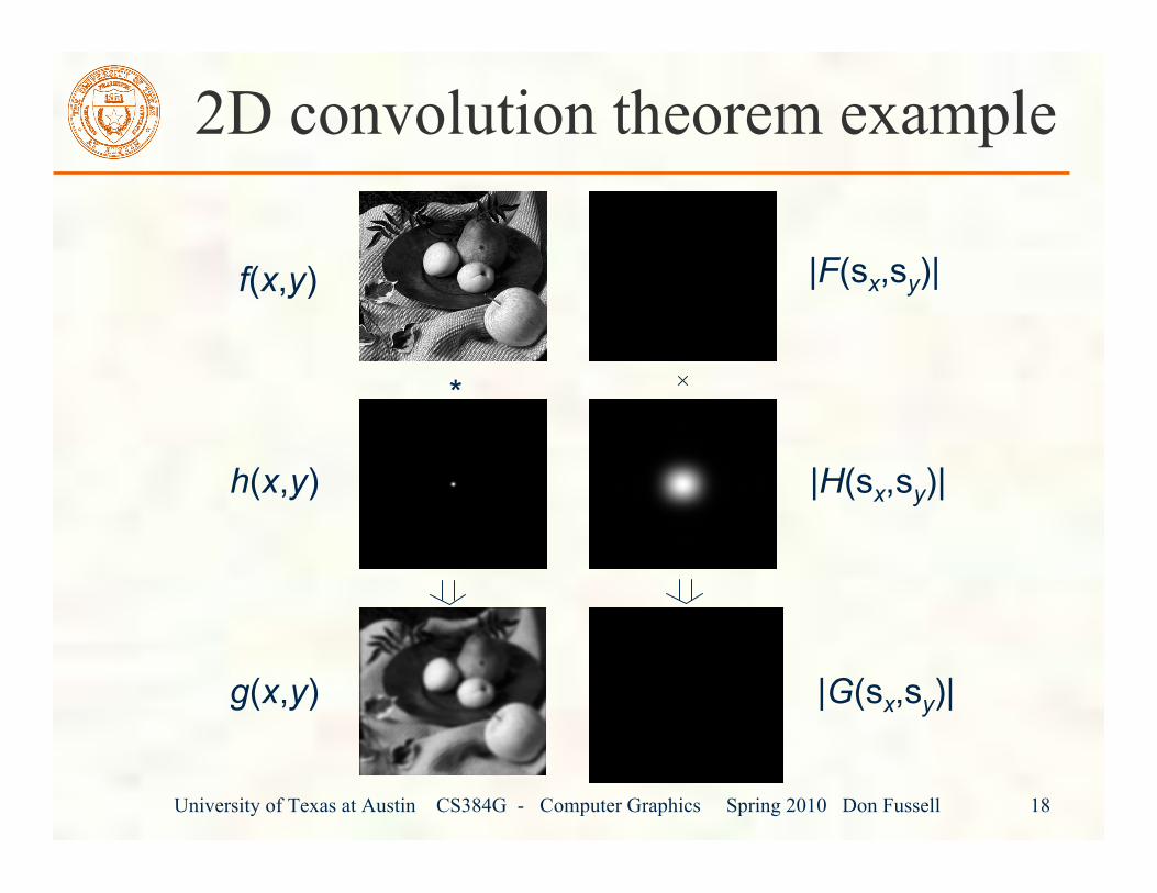
Convolution theorem: Convolution in thespatial domain is equivalent tomultiplication in the frequency domain.

Symmetric theorem: Convolution in thefrequency domain is equivalent tomultiplication in the spatial domain.!

f " h# F $H

!

f " h# F $H


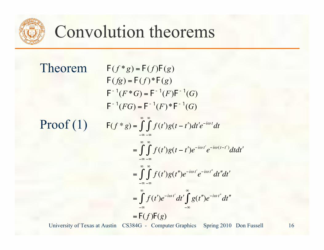
Convolution theorems

Theorem

Proof (1))(*)()(

)()()*(

)(*)()(

)()()*(

GFFG

GFGF

gffg

gfgf

1-1-1-

1-1-1-

FFF

FFF

FFF

FFF

=

=

=

=

!

F( f * g) = f ( " t )g(t # " t )d " t e#i$ t

dt#%

%

&#%

%

&

= f ( " t )g(t # " t )e# i$ " t

e# i$ ( t# " t )

dtd " t #%

%

&#%

%

&

= f ( " t )g( " " t )e# i$ " t

e# i$ " " t

d " " t d " t #%

%

&#%

%

&

= f ( " t )e# i$ " t

d " t g( " " t )e#i$ " " t

d " " t #%

%

&#%

%

&

= F( f )F(g)


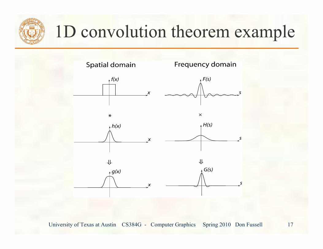
1D convolution theorem example


2D convolution theorem example

*

f(x,y)

h(x,y)

g(x,y)

|F(sx,sy)|

|H(sx,sy)|

|G(sx,sy)|


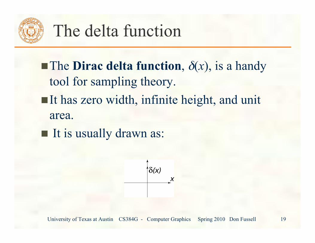
The delta function

The Dirac delta function, δ(x), is a handytool for sampling theory.It has zero width, infinite height, and unitarea. It is usually drawn as:


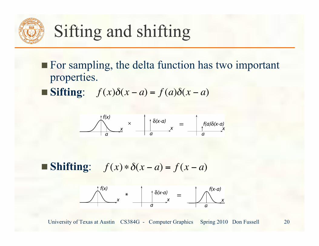
Sifting and shifting

For sampling, the delta function has two importantproperties.Sifting:

Shifting:

!

f (x)"(x # a) = f (a)"(x # a)

!

f (x)"#(x $ a) = f (x $ a)


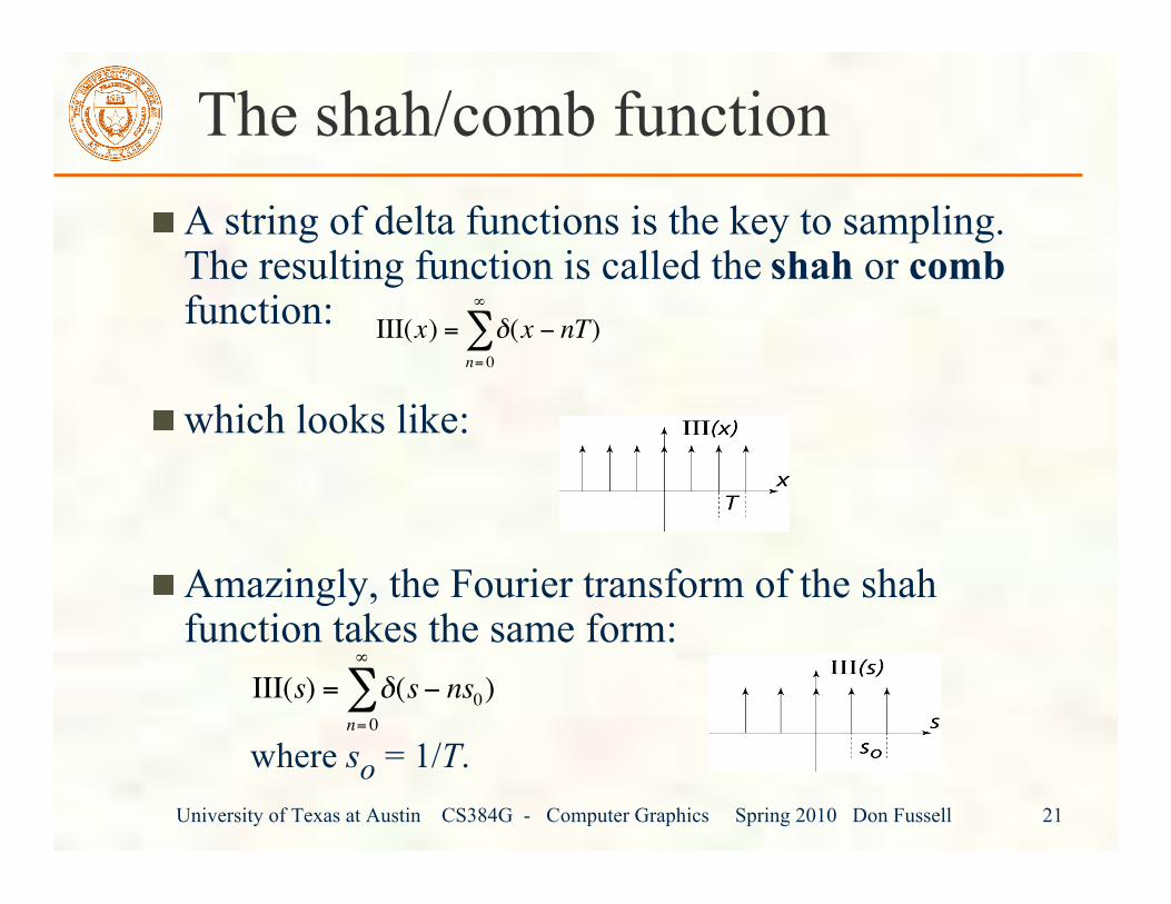
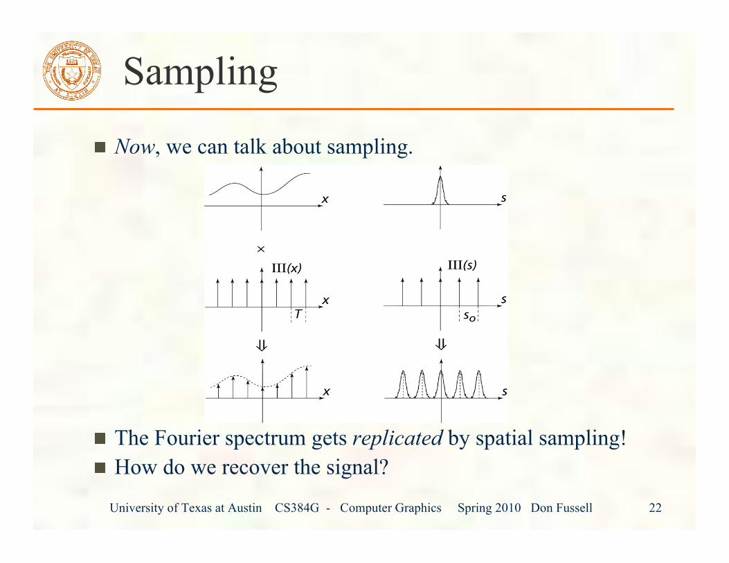
The shah/comb functionA string of delta functions is the key to sampling.The resulting function is called the shah or combfunction:

which looks like:

Amazingly, the Fourier transform of the shahfunction takes the same form:

where so = 1/T.

!

III(x) = "(x # nT)n= 0

$

%

!

III(s) = "(s# ns0)

n= 0

$

%


Now, we can talk about sampling.

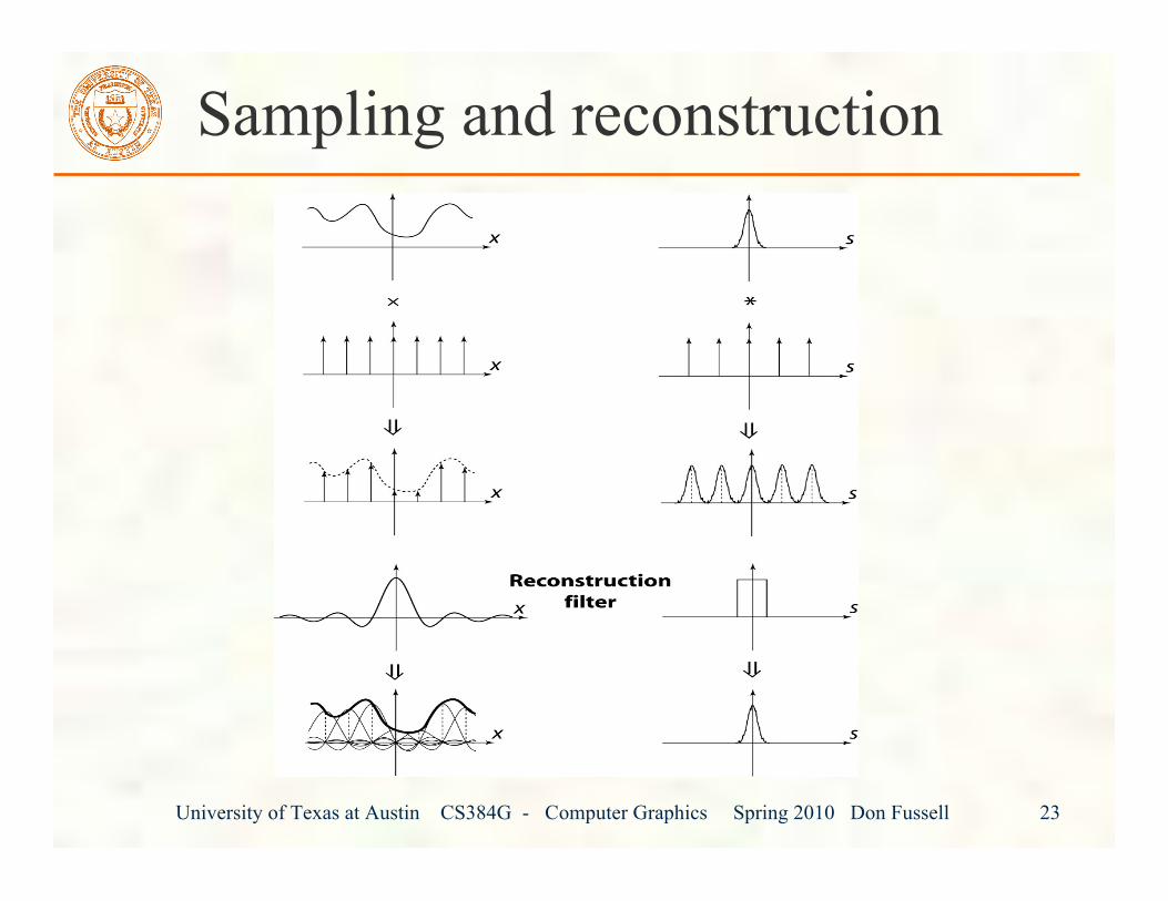
The Fourier spectrum gets replicated by spatial sampling!How do we recover the signal?

Sampling


Sampling and reconstruction


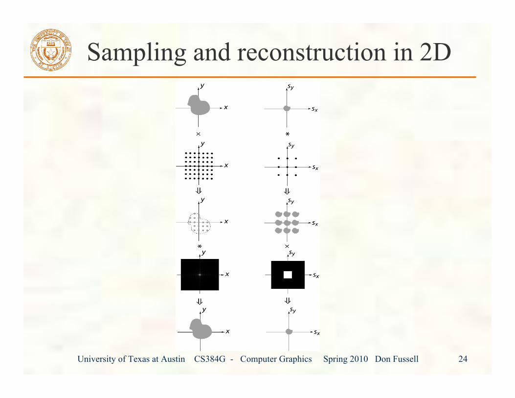
Sampling and reconstruction in 2D


Sampling theorem

This result is known as the Sampling Theoremand is generally attributed to Claude Shannon(who discovered it in 1949) but was discoveredearlier, independently by at least 4 others:A signal can be reconstructed from its samples without

loss of information, if the original signal has no energy infrequencies at or above ½ the sampling frequency.For a given bandlimited function, the minimumrate at which it must be sampled is the Nyquistfrequency.


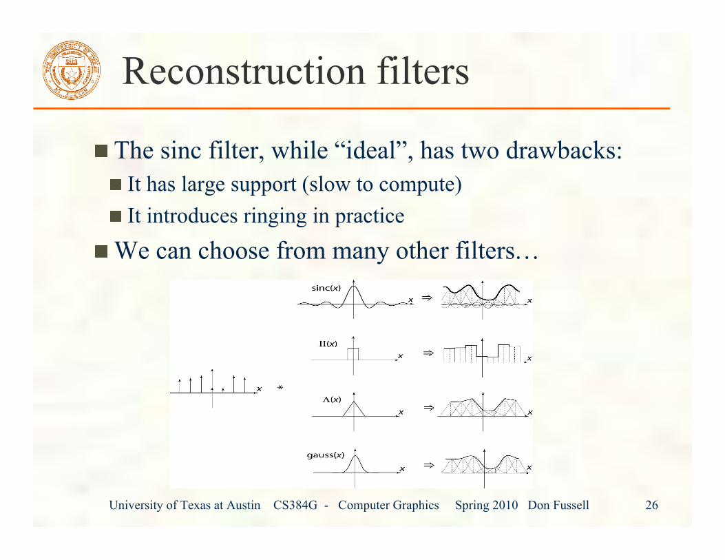
Reconstruction filters

The sinc filter, while “ideal”, has two drawbacks: It has large support (slow to compute) It introduces ringing in practice

We can choose from many other filters…


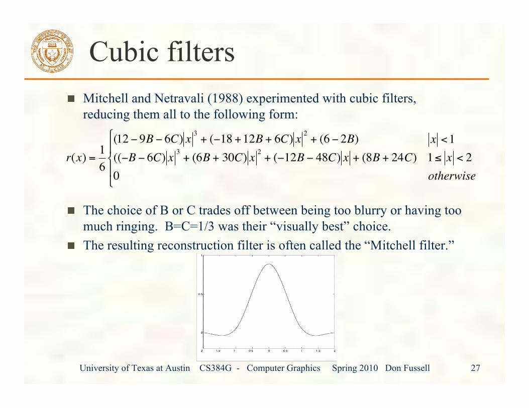
Cubic filtersMitchell and Netravali (1988) experimented with cubic filters,reducing them all to the following form:

The choice of B or C trades off between being too blurry or having toomuch ringing. B=C=1/3 was their “visually best” choice.The resulting reconstruction filter is often called the “Mitchell filter.”

!

r(x) =1

6

(12 " 9B " 6C) x3

+ ("18 +12B + 6C) x2

+ (6 " 2B)

(("B " 6C) x3

+ (6B + 30C) x2

+ ("12B " 48C) x + (8B + 24C)

0

#

$ %

& %

x <1

1' x < 2

otherwise


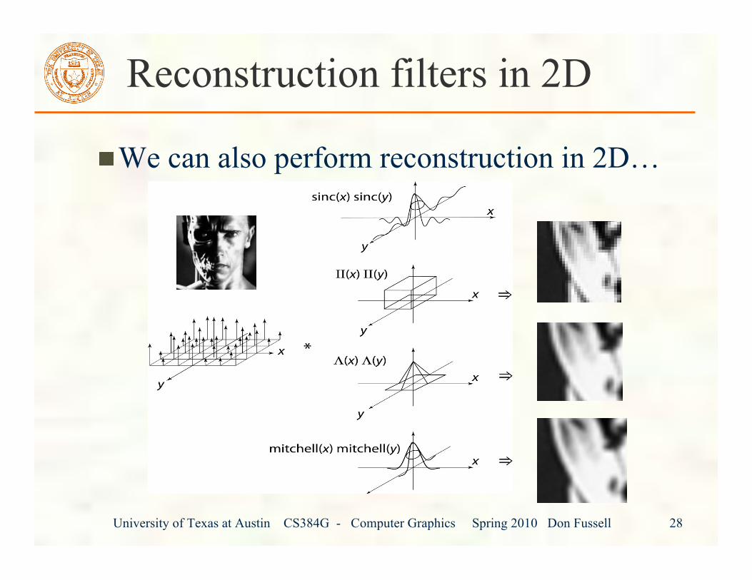
Reconstruction filters in 2D

We can also perform reconstruction in 2D…


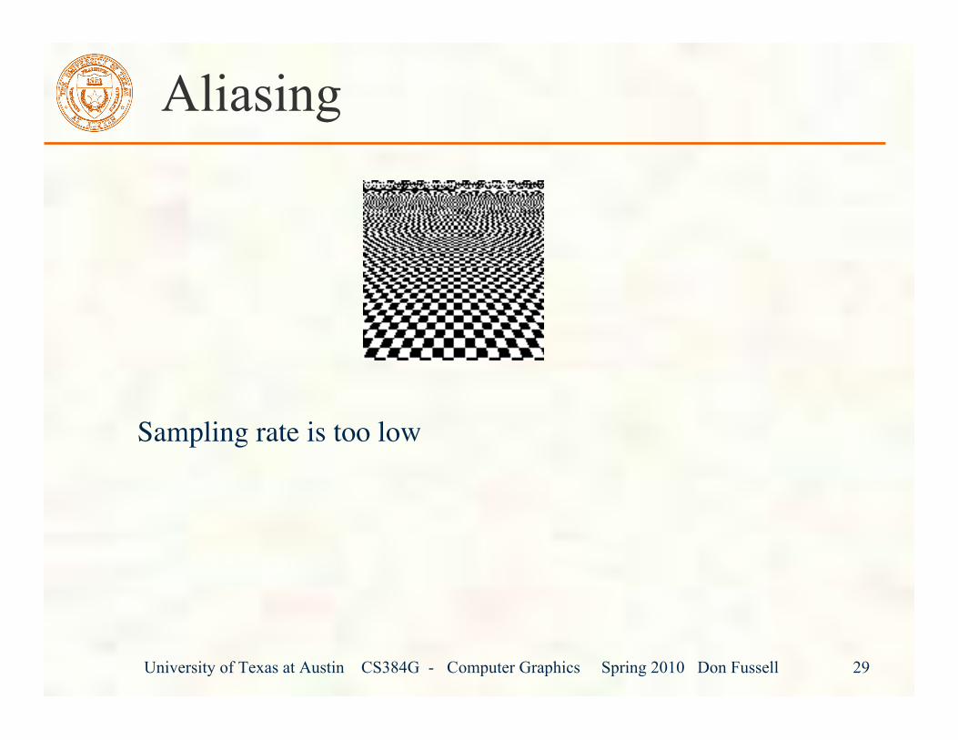
Aliasing

Sampling rate is too low


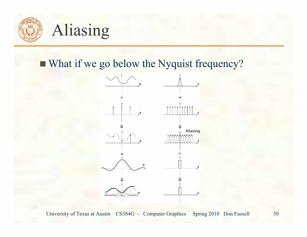
Aliasing

What if we go below the Nyquist frequency?


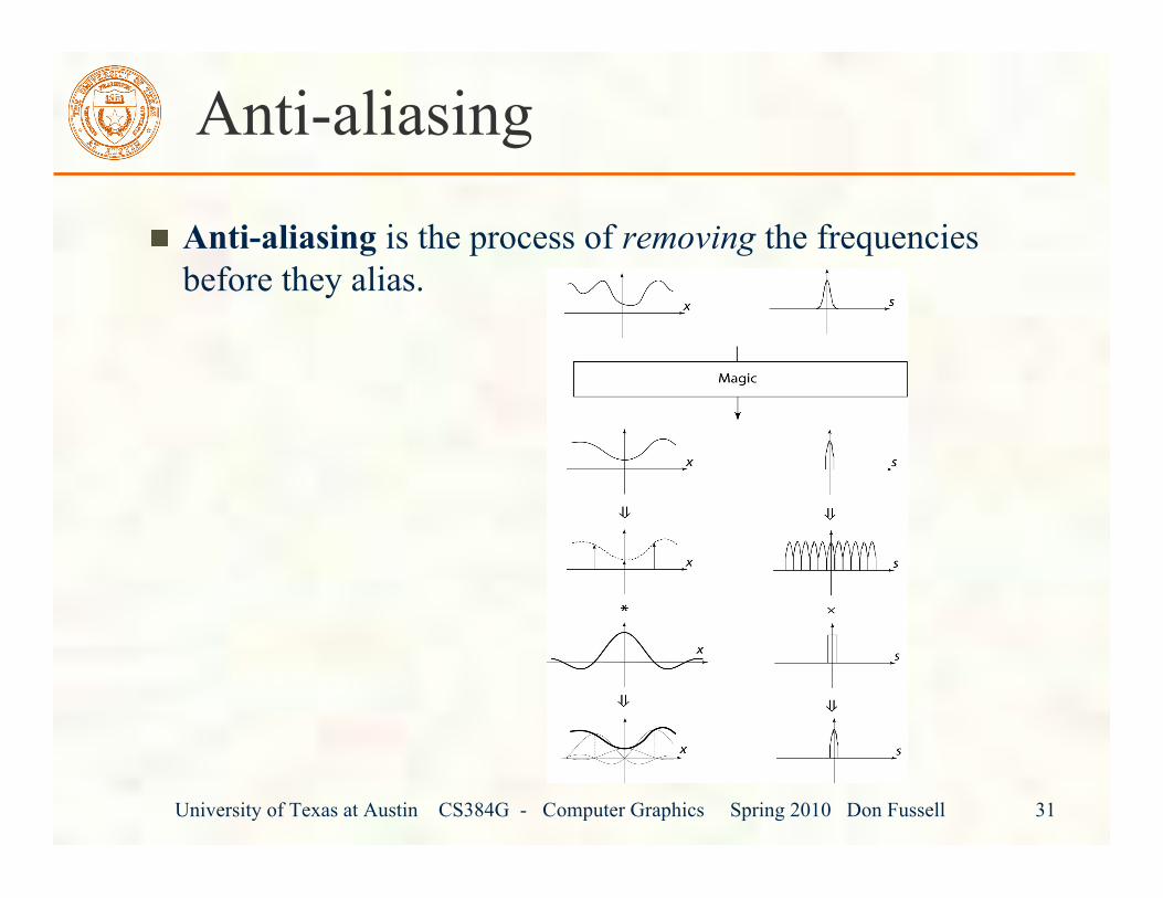
Anti-aliasing

Anti-aliasing is the process of removing the frequenciesbefore they alias.


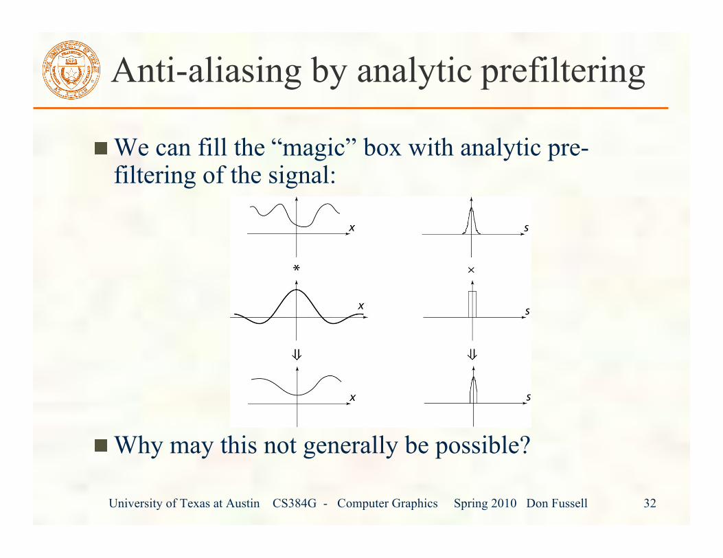
We can fill the “magic” box with analytic pre-filtering of the signal:

Why may this not generally be possible?

Anti-aliasing by analytic prefiltering


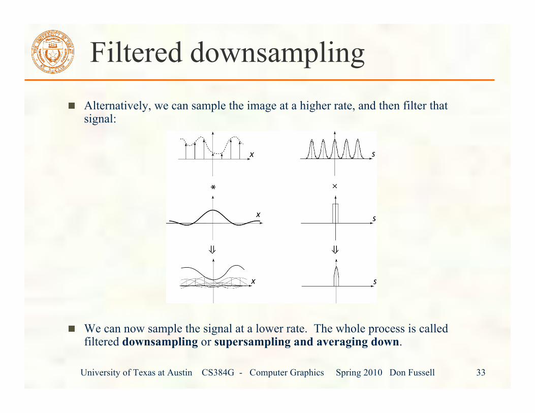
Filtered downsamplingAlternatively, we can sample the image at a higher rate, and then filter thatsignal:

We can now sample the signal at a lower rate. The whole process is calledfiltered downsampling or supersampling and averaging down.


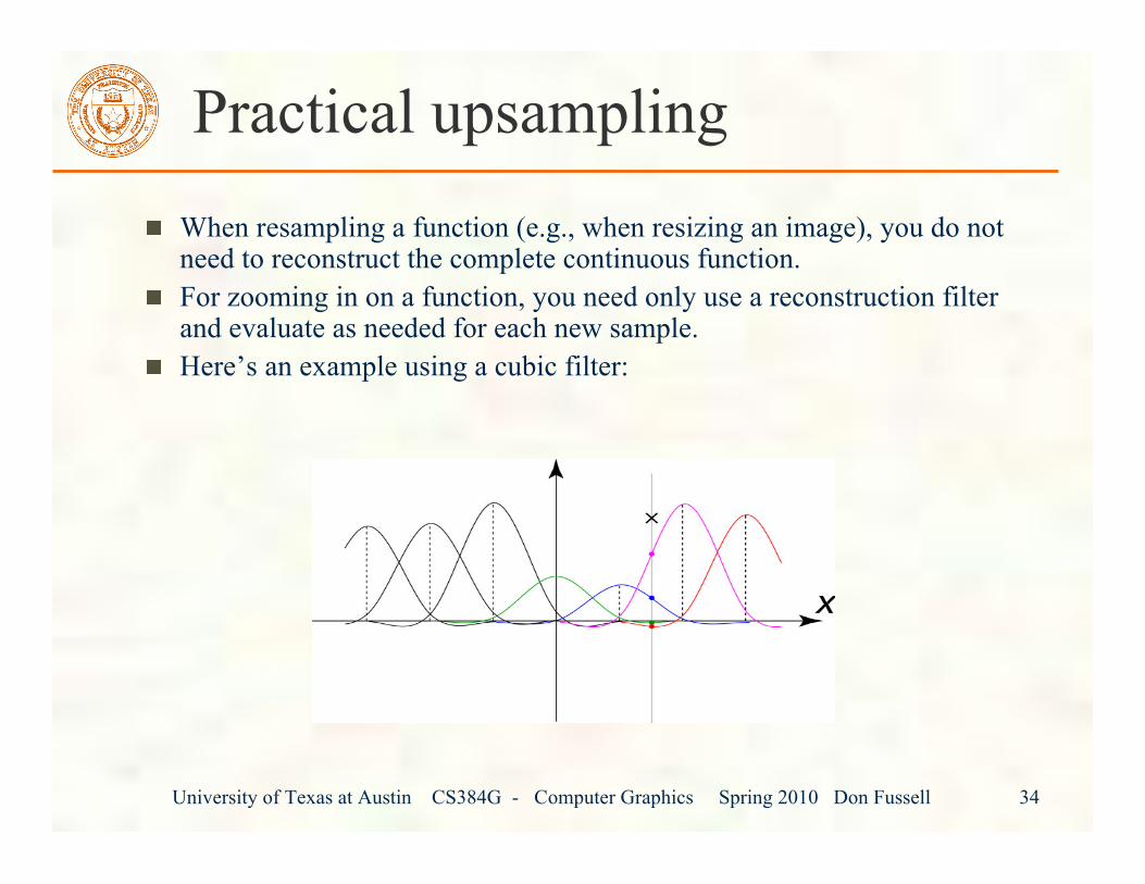
Practical upsamplingWhen resampling a function (e.g., when resizing an image), you do notneed to reconstruct the complete continuous function.For zooming in on a function, you need only use a reconstruction filterand evaluate as needed for each new sample.Here’s an example using a cubic filter:


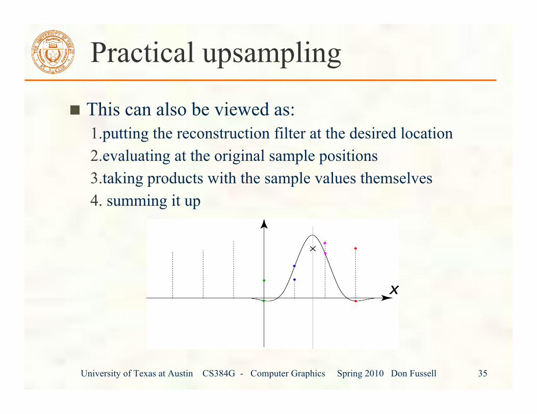
Practical upsampling

This can also be viewed as:1.putting the reconstruction filter at the desired location2.evaluating at the original sample positions3.taking products with the sample values themselves4. summing it up

Important: filter should always be normalized!


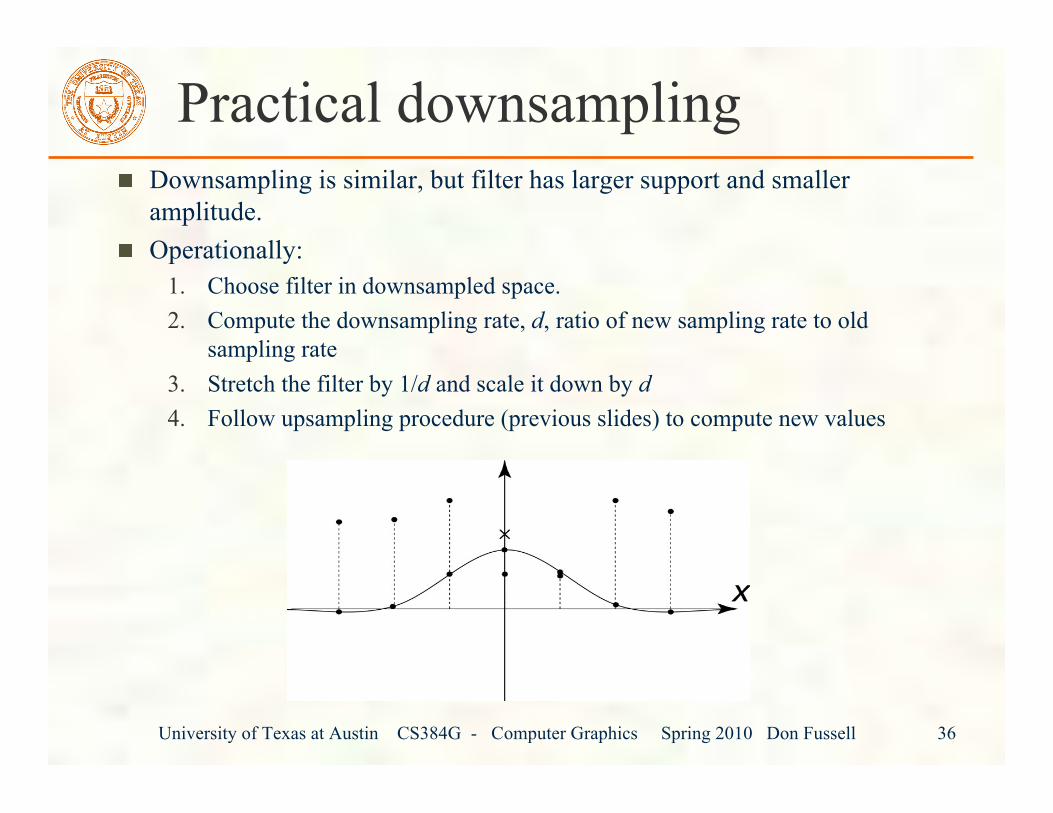
Practical downsamplingDownsampling is similar, but filter has larger support and smalleramplitude.Operationally:

1. Choose filter in downsampled space.2. Compute the downsampling rate, d, ratio of new sampling rate to old

sampling rate3. Stretch the filter by 1/d and scale it down by d4. Follow upsampling procedure (previous slides) to compute new values


2D resamplingWe’ve been looking at separable filters:

How might you use this fact for efficient resampling in 2D?!

r2D (x,y) = r

1D (x)r1D (y)


Next class: Image Processing

Reading:Jain, Kasturi, Schunck, Machine Vision.McGraw-Hill, 1995.Sections 4.2-4.4, 4.5(intro), 4.5.5, 4.5.6, 5.1-5.4. (from course reader)

Topics:- Implementing discrete convolution- Blurring and noise reduction- Sharpening- Edge detection

Documents

Sampling and Reconstruction - cs.utexas.eduSampling and Reconstruction. University of Texas at Austin CS384G - Computer Graphics Spring 2010 Don Fussell 2 Reading ... What is an image?