Scheduling parallel machines with major and minor setup times

The International Journal of Flexible Manufacturing Systems, 2 (1990): 329-341 �9 1990 Kluwer Academic Publishers, Boston. Manufactured in The Netherlands.

Scheduling Parallel Machines with Major and Minor Setup Times

ROBERT J. WITTROCK Manufacturing Research Department, IBM Thomas J. Watson Research Center, PO. Box 218, Yorktown Heights, NY 10598

Abstract. This article discusses the problem of scheduling a large set of parts on an FMS so as to minimize the total completion time. Here, the FMS consists of a set of parallel identical machines. Setup time is incurred whenever a machine switches from one type of part to another. The setup time may be large or small depending on whether or not the two part types belong to the same family. This article describes a fast heuristic for this scheduling problem and derives a lower bound on the optimal solution. In computational tests using random data and data from an IBM card test line, the heuristic archieves nearly optimal schedules.

Key Words: Scheduling, parallel machines, major and minor setup times, heuristics.

I. Introduction

Consider a flexible manufacturing system (FMS) that performs operations on a large set of parts. Each part can be processed by any one of several identical machines. There are numerous different types of parts to be processed (part types). The time for a machine to process one part is very short and depends only on the part type. A machine incurs a minor setup time (of moderate length) whenever it switches from one part type to another. The length of this minor setup time depends only on the part type being switched to. The part types are grouped into families. When a machine switches part types, if the part types belong to different families, the machine incurs a long, major setup time, in addition to the minor setup time. The length of this major setup time depends only on the family being switched to. The problem addressed is to schedule the parts on the machines so as to minimize the makespan, which is the time necessary to complete all the parts. In what follows, this problem will be called MMSS, major and minor setup scheduling.

Previous work related to this problem includes several papers on scheduling parallel machines with setup costs and an overall cost objective, e.g., Geoffrion and Graves (1976). Unfortu- nately, this work does not appear to apply to scheduling with setup times and a makespan objective. Scheduling a single machine with arbitrary sequence-dependent setup times with a makespan objective is equivalent to the traveling salesman problem (Lawler et al. 1985).

Scheduling parallel machines with no setups and a makespan objective is a well-studied problem. The problem is NP-hard (Ullman, 1976), and so it appears that any algorithm that computes an optimal schedule must take an exponentially long run time. For this reason, heuristic algorithms have been proposed that compute near-optimal schedules in polynomial time. These include the Longest-Process-Time-First rule analyzed by Graham (1969), the

330 ROBERT J. WITTROCK

MULTIFIT heuristic of Coffman et al. (1978), and the polynomial approximation scheme of Hochbaum and Shmoys (1987). In these papers, the heuristics are evaluated by deriving a worst-case performance bound on the ratio of the heuristic makespan to the optimum. Both the MULTIFIT heuristic and the approximation scheme use a binary search on the makespan in order to reduce the parallel-machine scheduling problem to the bin-packing problem, which is, in some sense, dual to the scheduling problem.

Dietrich (1989) has developed a heuristic for the problem of scheduling parallel unrelated machines with setups (PUMS). In some sense, the PUMS problem is more general than the MMSS problem because the machines are unrelated, i.e., the process time and setup time for a part type depend, in an arbitrary way, on the machine to which the part type is assigned. Also, the objective is a weighted average of makespan and mean flow time. In another sense, PUMS is less general than MMSS, because it considers only one class of setup times, as opposed to the two classes (major and minor) that characterize the MMSS problem.

The MMSS problem is also NP-hard (see below). It has previously been addressed in Tang and Wittrock (1985) and Tang (1988). These papers develop a heuristic for the problem based on the MULTIFIT heuristic.

The present article develops a new heuristic, which also uses the binary search approach of MULTIFIT. Section 2 gives two examples of the MMSS problem in FMSs. Section 3 describes the heuristic. Section 4 derives a lower bound on the optimal makespan. Section 5 describes the results of computational tests using random data. On the average, the heuristic came within 3 % of the lower bound on the optimal makespan. Section 6 describes the results of computational tests using data from an IBM card test line. In this case, the heuristic performed even better than on the random problems. In an appendix, the tests of section 5 are extended in order to compare the heuristic and the bound with those of Tang and Wittrock. The tests show improvement in both respects.

M

N = H = ~ =

tk= S k

r j =

The MMSS problem can be defined by the following data. Let the number of machines the number of families the number of part types the family to which part type k belongs {kljk = j} = the set of part types that compose family j the total process time of all parts of type k the minor setup time to switch to part type k the major setup time to switch to family j

It is assumed that the process time for an individual part is so small compared to the minor setup time that it need not be explicitly considered. What matters is the total process time, t k, which can be partitioned arbitrarily into batches, at the cost of one minor setup time per batch. This assumption makes the problem easier to solve heuristically, although it is still NP-hard. All data are integers, and it is assumed that each machine will spend an integral amount of time processing each part type.

Notice that no machine needs to process more than one batch of the same part type. A schedule that puts two or more batches of the same type on the same machine can always be improved (or made no worse) by combining the batches into one, thereby eliminating

SCHEDULING PARALLEL MACHINES WITH MAJOR AND MINOR SETUP TIMES 331

a setup. The same observation also applies to families. All part types of the same family that a machine processes should be processed consecutively. Also notice that it does not matter in what order the families on one machine are processed. Similarly, it does not matter in what order the part types within one family are processed on a machine as long as they are processed consecutively. Thus the sequencing aspect of this scheduling problem is trivial. What remains is an allocation problem, namely, determining which part types should be processed on each machine and how much time each machine should spend on each part type.

The objective is to minimize the makespan, which is the time to process all the parts. Define the work load of a machine to be the total process time that has been allocated to it, plus the minor setup time of each part type that has been allocated to it plus the major setup time of each family that has been allocated to it. Then the makespan is the maximum of the machine work loads. Implicit in the makespan objective are two conflicting goals: work load balance and setup minimization. A schedule that optimizes one of these objectives would probably not optimize the other. The makespan objective provides an equitable means of trading off between these two objectives.

It is easy to show that the MMSS problem is NP-hard, by the following reduction from the problem of scheduling parallel identical machines without setups. Consider a general instance of the no-setup problem. There are H jobs and each job k has process time Pk. Construct the following MMSS problem instance: There is one family, and its major setup time is zero. There is one part type k for each job k in the no-setup problem, with t k = 1 and sk = Pk - 1. Since each machine must spend an integral amount of time processing each part type, it follows from this construction that each part type k will be processed by only one machine, which must spend Pk time units on setup and process time. Clearly this is equivalent to the no-setup problem.

2. Examples of the MMSS problem in FMSs

Typically, in a real FMS environment, scheduling is done on an ongoing basis. Periodically, a new set of parts arrives at the system and needs to be scheduled along with any parts that have not yet entered the system. In this case (the loaded case), the scheduling problem must take into account the current state of the system, including the current setup of each machine and any parts queuing for any machine. The definition of the MMSS problem is for the pure case in which no machine is set up and there are no parts already in the system. The heuristic described in this article could easily be extended to the loaded case, but for ease of exposition, all discussion will be for the pure case, except when otherwise noted.

When scheduling in an ongoing environment, an appropriate objective would be to maximize the long-run throughput rate, i.e., the number of parts produced per unit time. How- ever, when scheduling a finite set of parts, a reasonable approximation is to maximize the throughput rate of those parts, i.e.,

Number of parts. Makespan

Since the number of parts is fixed, this is equivalent to minimizing the makespan.


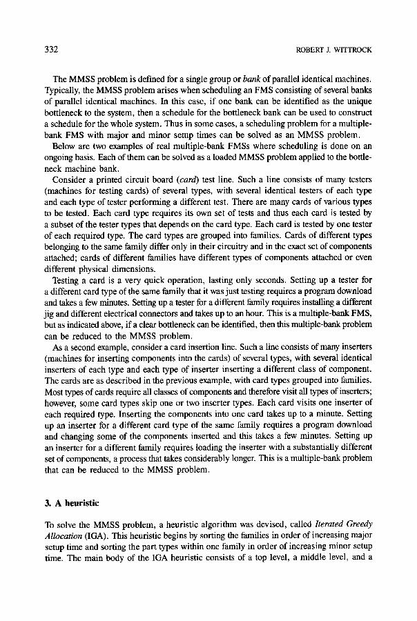
The MMSS problem is defined for a single group or bank of parallel identical machines. Typically, the MMSS problem arises when scheduling an FMS consisting of several banks of parallel identical machines. In this case, if one bank can be identified as the unique bottleneck to the system, then a schedule for the bottleneck bank can be used to construct a schedule for the whole system. Thus in some cases, a scheduling problem for a multiple- bank FMS with major and minor setup times can be solved as an MMSS problem.

Below are two examples of real multiple-bank FMSs where scheduling is done on an ongoing basis. Each of them can be solved as a loaded MMSS problem applied to the bottleneck machine bank.

Consider a printed circuit board (card) test line. Such a line consists of many testers (machines for testing cards) of several types, with several identical testers of each type and each type of tester performing a different test. There are many cards of various types to be tested. Each card type requires its own set of tests and thus each card is tested by a subset of the tester types that depends on the card type. Each card is tested by one tester of each required type. The card types are grouped into families. Cards of different types belonging to the same family differ only in their circuitry and in the exact set of components attached; cards of different families have different types of components attached or even different physical dimensions.

Testing a card is a very quick operation, lasting only seconds. Setting up a tester for a different card type of the same family that it was just testing requires a program download and takes a few minutes. Setting up a tester for a different family requires installing a different jig and different electrical connectors and takes up to an hour. This is a multiple-bank FMS, but as indicated above, if a clear bottleneck can be identified, then this multiple-bank problem can be reduced to the MMSS problem.

As a second example, consider a card insertion line. Such a line consists of many inserters (machines for inserting components into the cards) of several types, with several identical inserters of each type and each type of inserter inserting a different class of component. The cards are as described in the previous example, with card types grouped into families. Most types of cards require all classes of components and therefore visit all types of inserters; however, some card types skip one or two inserter types. Each card visits one inserter of each required type. Inserting the components into one card takes up to a minute. Setting up an inserter for a different card type of the same family requires a program download and changing some of the components inserted and this takes a few minutes. Setting up an inserter for a different family requires loading the inserter with a substantially different set of components, a process that takes considerably longer. This is a multiple-bank problem that can be reduced to the MMSS problem.

3. A heuristic

To solve the MMSS problem, a heuristic algorithm was devised, called Iterated Greedy Allocation (IGA). This heuristic begins by sorting the families in order of increasing major setup time and sorting the part types within one family in order of increasing minor setup time. The main body of the IGA heuristic consists of a top level, a middle level, and a


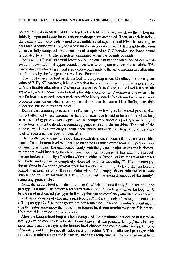
bottom level. As in MULTI-FIT, the top level of IGA is a binary search on the makespan. Initially, upper and lower bounds on the makespan are computed. Then, at each iteration, the mean of the two bounds is used as a candidate makespan, T, and IGA tries to compute a feasible allocation for T, i.e., one whose makespan does not exceed T. I fa feasible allocation is successfully computed, the upper bound is updated to T. Otherwise, the lower bound is updated to T + 1. The search is terminated when the bounds coincide.

Zero will suffice as an initial lower bound, or one can use the lower bound derived in section 4. For an initial upper bound, it suffices to compute any feasible schedule. This can be done by allocating all part types within one family to the same machine and allocating the families by the Longest-Process Time First rule.

The middle level of IGA is its method of computing a feasible allocation for a given value of T. By NP-hardness, it is unlikely that there is a fast algorithm that is guaranteed to find a feasible allocation of Twhenever one exists. Instead, the middle level is a heuristic approach, which seems likely to find a feasible allocation for T whenever one exists. The middle level is executed once at each step of the binary search. Which way the binary search proceeds depends on whether or not the middle level is successful at finding a feasible allocation for the current value of T.

Define the remaining process time of a part type or family to be its total process time not yet allocated to any machine. A family or part type is said to be unallocated as long as its remaining process time is positive. To completely allocate a part type or family to a machine is to allocate all its remaining process time to the machine. The goal of the middle level is to completely allocate each family and each part type, so that the work load of each machine does not exceed T.

The middle level consists of a loop that, at each iteration, chooses a family j and a machine i and calls the bottom level to allocate to machine i as much of the remaining process time of family j as it can. The unallocated family with the greatest major setup time is chosen, in order to avoid incurring this setup time more than necessary. (Here and in the sequel, ties are broken arbitrarily.) To define which machine is chosen, let I be the set of machines to which family j can be completely allocated (without exceeding /). I f I is nonempty, the machine in I with the greatest work load is chosen, in order to leave the less heavily loaded machines for other families. Otherwise, if I is empty, the machine of least work load is chosen. This machine will be able to absorb the greatest amount of the family's remaining process time.

Next, the middle level calls the bottom level, which allocates family j to machine i, one part type at a time. The bottom level starts with a loop. At each iteration of the loop, let K be the set of unallocated part types in family j that can be completely allocated to machine i. The iteration consists of choosing a part type k E K and completely allocating it to machine i. The part type k e K with the greatest minor setup time is chosen, in order to avoid incurring this setup time more than once. The bottom-level loop terminates when K is empty. Note that this may occur immediately.

After the bottom-level loop has been completed, no remaining unaUocated part type in family j can be completely allocated to machine i. At this point, if family j includes any more unallocated part types, the bottom level chooses one more unallocated part type k of family j and tries to partially allocate it to machine i. The unallocated part type with the smallest minor setup time is chosen, since this setup time will be incurred on at least


two machines. I f it is possible to allocate any of the remaining process time of part type k to machine i, just enough process time from part type k is allocated so that the work load of machine i equals T. Otherwise there is no room for any more allocation from family j and none is performed. This completes the bottom level.

Executing the bottom level completes one iteration of the middle-level loop. There are two ways that the middle level can terminate. It is possible to complete a full iteration of the middle-level loop without allocating any process time. In this case, the middle level is not able to do any more allocating, and so it terminates. This is the unsuccessful case, and T is increased at the next iteration of the binary search. Otherwise, the middle-level loop terminates when all families have been completely allocated. This is the successful case, and Tis decreased at the next iteration of the binary search. This completes the definition of IGA.

To calculate the complexity of IGA, first note that the initial sorting step runs in O(Hlog(H)) time, which is dominated by the run time of the main body of the algorithm.

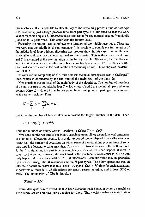
Now consider the top level of the main body of the algorithm. The number of iterations of a binary search is bounded by log(U - L), where U and L are the initial uper and lower bounds. Here, L = 0, and U can be computed by assuming that all part types are allocated to the same machine. Thus

j k

Let G = the number of bits it takes to represent the largest number in the data. Then

U _.< 3H(26") -< 3(226)

Thus the number of binary search iterations is O0og(U)) = O(G). Now consider the run time of one binary search iteration. Since the middle level terminates

as soon as no allocation occurs, it is useful to bound the number of times allocation can occur, i.e., the number of occasions on which some of the remaining process time of some part type is allocated to some machine. This occurs in two situations in the bottom level. In the first situation, the part type is completely allocated. This can happen at most H times. In the second situation, the work load of the machine is made equal to T. This can only happen M times, for a total of H + M allocations. Each allocation may be preceded by a search through the M machines and the H part types. The other operations that an allocation entails are faster than this. Thus IGA spends O(H + M) time for each allocation, it performs at most H + M allocations per binary search iteration, and it does O(G) of these. The complexity of IGA is therefore

O(G(H + M)2).

It would be quite easy to extend the IGA heuristic to the loaded case, in which the machines are already set up and have parts queuing for them. This would involve an initialization


step to the middle level. First, each machine would be assigned an initial work load corresponding to its queue of parts. Then, families and part types would be assigned to machines for which they set up. After this, the middle level would proceed normally.

4. A b o u n d

To evaluate the IGA heuristic, computational tests were performed, and these are described in sections 5 and 6. Ideally, such tests would compare the heuristic makespan to the optimal makespan, but since the optimal makespan is difficult to obtain, a lower bound on the optimal makespan was used instead.

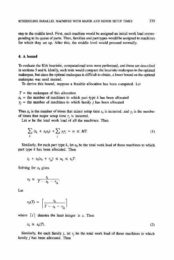
To derive this bound, suppose a feasible allocation has been computed. Let

T = the makespan of this allocation Xk = the number of machines to which part type k has been allocated yj = the number of machines to which family j has been allocated

Thus Xk is the number of times that minor setup time Sk is incurred, and yj is the number of times that major setup time rj is incurred.

Le t w be the total work load of all the machines. Then

~ a (tk + xksD + ~_a yjrj = w < MT. (1) k j

Similarly, for each part type k, let uk be the total work load of those machines to which part type k has been allocated. Then

tk + xk(s~ + ~k) <- uk <-- xgT.

Solving for Xk gives

tk Xk-----

T - - sk -- rjk"

Let

T - - S k -- rj

where I-z-] denotes the least integer _> z. Then

x~ ~ x~(T~. (2)

Similarly, for each family j , let vj be the total work load of those machines to which family j has been allocated. Then

336 ROBERT J. W l T T R O C K

(tk + X:k) + 3917 <_ ~9 <- Y1T.

Solving for 39 gives

Let

Then

Yj >- tI~_ rjl Z (tk + XkSk)' k~rj

Y J(73 = I tl--f--~--rjl~a(tk+Xk(I)Sk)]" ~Xj

39 ~ yj(7). (3)

Applying inequalities (2) and (3) to inequality (1) gives

(t k + x~(T)Sk) + ~_a yj(T)rj < MT. (4) k j

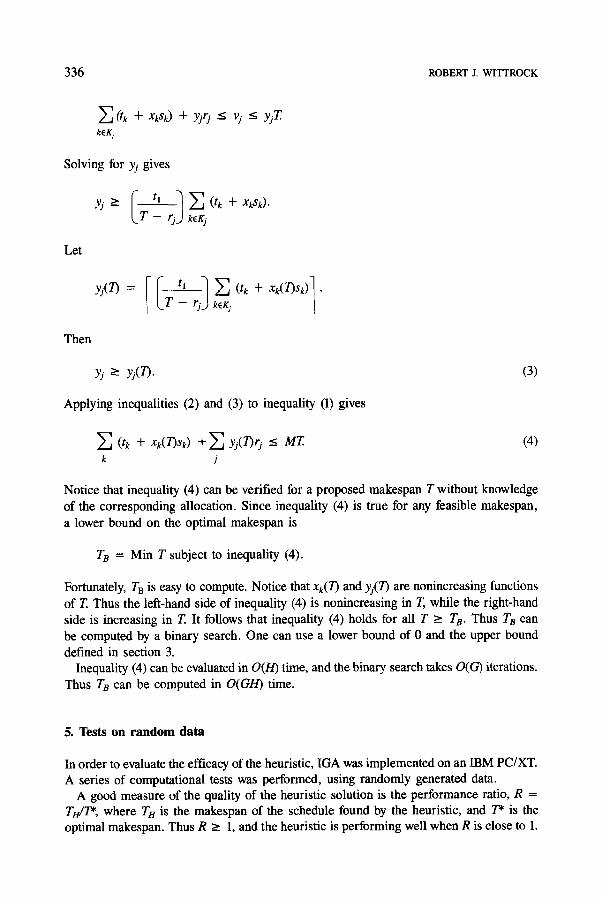
Notice that inequality (4) can be verified for a proposed makespan T without knowledge of the corresponding allocation. Since inequality (4) is true for any feasible makespan, a lower bound on the optimal makespan is

TB = Min T subject to inequality (4).

Fortunately, TB is easy to compute. Notice that x,(/) and yj(/) are nonincreasing functions of T. Thus the left-hand side of inequality (4) is nonincreasing in T, while the right-hand side is increasing in T. It follows that inequality (4) holds for all T _> T B. Thus TB can be computed by a binary search. One can use a lower bound of 0 and the upper bound defined in section 3.

Inequality (4) can be evaluated in O(/-/) time, and the binary search takes O(G) iterations. Thus TB can be computed in O(GH) time.

5. Tests on random data

In order to evaluate the efficacy of the heuristic, IGA was implemented on an IBM PC/XT. A series of computational tests was performed, using randomly generated data.

A good measure of the quality of the heuristic solution is the performance ratio, R = TIt~T*, where TIt is the makespan of the schedule found by the heuristic, and T* is the optimal makespan. Thus R >_ 1, and the heuristic is performing well when R is close to 1.


Since the optimal makespan was not readily available, the lower bound, To, was used to compute the performance bound, Ro = TI4/TB. Thus 1 < R < RB, so the performance bound is a conservative estimate of the performance ratio.

Several groups of random problems were generated according to the following parameters:

�9 M = 5, 8, or 12, depending on the group �9 N = 5, 10, or 15, depending on the group �9 ]Kil, the number of part types for each family j , was uniformly distributed over [1, 10] �9 Each Sk was uniformly distributed over [1, 10] �9 Each r: was uniformly distributed over [20, 50] or [30, 80], depending on the group �9 Each tk was uniformly distributed over [20, 60] or [30, 90], depending on the group

All random values were independent. Thus there were three cases for M, three for N, two for rj, and two for tk, for a total

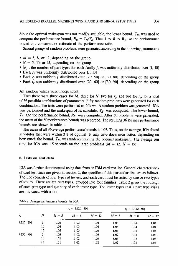
of 36 possible combinations of parameters. Fifty random problems were generated for each combination. The tests were performed as follows. A random problem was generated. IGA was performed and the makespan of its schedule, TH, was computed. The lower bound, To, and the performance bound, RB, were computed. After 50 problems were generated, the mean of the 50 performance bounds was recorded. The resulting 36 average performance bounds are shown in table 1.

The mean of all 36 average performance bounds is 1.03. Thus, on the average, IGA found schedules that were within 3 % of optimal. It may have doen even better, depending on how much the bound, To, was underestimating the optimal makespan. The average run time for IGA was 1.5 seconds on the large problems (M = 12, N = 15).

6. Tests on real data

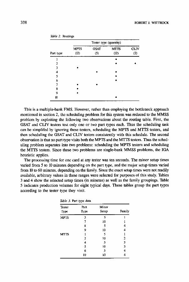
IGA was further demonstrated using data from an IBM card test line. General characteristics of card test lines are given in section 2; the specifics of this particular line are as follows. The line consists of four types of testers, and each card must be tested by one or two types of testers. There are ten part types, grouped into four families. Table 2 gives the routings of each part type and quantity of each tester type. The tester types that a part type visits are indicated with a dot.

T a b l e 1. Average performance bounds for IGA

tk N

r j - U[20, 50] r j - U[30, 80]

M = 5 M = 8 M = 12 M = 5 M = 8 M = 12

U[20, 60]

0[30, 90]

5 1.02 1.03 1.04 1.03 1.04 1.04 10 1.03 1.03 1.04 1.04 1.04 1.04 15 1.02 1.03 1.03 1.03 1.04 1.04 5 1.03 1.02 1.03 1.02 1.03 1.03 10 1.02 1.02 1,03 1.03 1.03 1.03 15 1.01 1.02 1,02 1.02 1.03 1,03

338 ROBERT J. WlTTROCK

Table 2. Routings

Part type

1 2 3 4 5 6 7 8 9

10

Tester type (quantity)

MPTS GSAT MTTS CLIV (12) (5) (12) (2)

This is a multiple-bank FMS. However, rather than employing the bottleneck approach mentioned in section 2, the scheduling problem for this system was reduced to the MMSS problem by exploiting the following two observations about the routing table. First, the GSAT and CLIV testers test only one or two part types each. Thus the scheduling task can be simplifed by ignoring these testers, scheduling the MPTS and MTTS testers, and then scheduling the GSAT and CLIV testers consistently with this schedule. The second observation is that no part type visits both the MPTS and the MTTS testers. Thus the scheduling problem separates into two problems: scheduling the MPTS testers and scheduling the MTTS testers. Since these two problems are single-bank MMSS problems, the IGA heuristic applies.

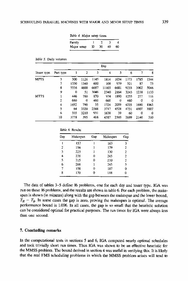
The processing time for one card at any tester was ten seconds. The minor setup times varied from 5 to 10 minutes depending on the part type, and the major setup times varied from 10 to 60 minutes, depending on the family. Since the exact setup times were not readily available, arbitrary values in these ranges were selected for purposes of this study. Tables 3 and 4 show the selected setup times (in minutes) as well as the family groupings. Table 5 indicates production volumes for eight typical days. These tables group the part types according to the tester type they visit.

Table 3. Part type data

Tester Part Minor Type Type Setup Family

MPTS 3 5 1 7 10 1 8 5 4 9 10 4

MTTS 1 5 1 2 10 2 4 5 3 5 10 3 6 5 4

10 10 4


Table 5. Daily volumes

Table 4. Major setup times

Family 1 2 3 4 Major setup 10 30 40 60

Day

Tester type Part type 1 2 3 4 5 6 7 8

MPTS 3 300 1126 1145 1814 1034 1773 1785 1544 7 1330 1340 600 108 979 321 87 73 8 5336 4600 6687 11103 6681 9233 3902 5046 9 0 51 3046 2340 2164 3243 1238 1133

MTTS 1 446 760 870 974 1890 1255 277 116 2 660 0 460 660 0 460 0 0 4 1692 790 35 1724 2059 4235 1690 1063 5 64 3320 2588 3717 4528 4731 4907 3007 6 335 3210 931 1638 39 60 0 0

10 3778 395 408 4387 2503 2699 2140 310

Table 6. Results

Day Makespan Gap Makespan Gap

1 157 1 163 3 2 156 1 179 2 3 225 1 130 2 4 278 0 245 2 5 215 0 210 2 6 268 1 245 3 7 158 0 187 0 8 170 0 118 0

The data of tables 3-5 define 16 problems, one for each day and tester type. IGA was

run on these 16 problems, and the results are shown in table 6. For each problem, the make-

span is shown (in minutes) along with the gap between the makespan and the lower bound,

TH -- TB. In some cases the gap is zero, proving the makespan is optimal. The average

performance bound is 1.006. In all cases, the gap is so small that the heuristic solution

can be considered optimal for practical purposes. The run times for IGA were always less

than one second.

7. C o n c l u d i n g r e m a r k s

In the computational tests in sections 5 and 6, IGA computed nearly optimal schedules

and took trivially short run times. Thus IGA was shown to be an effective heuristic for

the MMSS problem. The bound derived in section 4 was useful in verifying this. It is likely

that the real FMS scheduling problems in which the MMSS problem arises will tend to

340 ROBERT J. WlTTROCK

have multiple banks of parallel identical machines and to require scheduling on an ongoing basis. It is trivial to extend the IGA heuristic to the loaded case required to perform scheduling on an ongoing basis. In some cases, particularly when there is a single bottleneck, the multiple-bank case can be solved by IGA by reduction to the single-bank case. However, the general problem of solving an MMSS-type problem in a multiple-bank FMS with more than one bottleneck remains a topic for further research.

Appendix: Compar i son to an earl ier approach

A different heuristic for the MMSS problem is described in Tang and Wittrock (1985) and Tang (1988). The earlier heuristic is similar to IGA in that it performs a binary search on the makespan and tries to find a feasible assignment for the given makespan at each iteration. However, in other respects, the two heuristics are substantially different. The fundamental difference is that, unlike IGA, the earlier heuristic solves the problem in two phases, each involving a binary search on the makespan. The first phase assigns families and the second phase assigns part types. In the first phase, it is assumed that each part type will incur one minor setup time. The actual number of minor setup times is only determined in the second phase. Thus the families are assigned without knowing the number of minor setup times that their part types will incur. IGA avoids this problem by allocating families and part types in a single integrated process, so that by the time a family has been allocated, all its part types have also been allocated and the number of minor setup times is determined. This was the primary motivation for developing a new heuristic, and it required completely redesigning what was done at each step of the binary search (the middle and bottom levels of IGA).

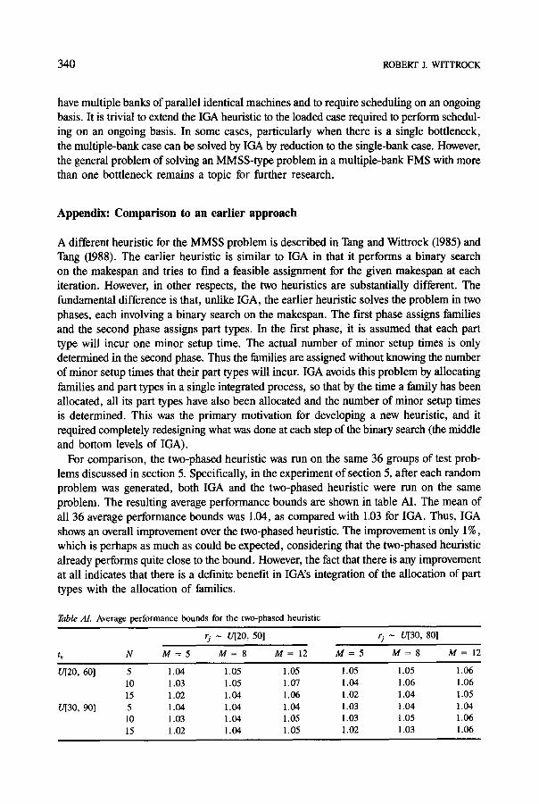
For comparison, the two-phased heuristic was run on the same 36 groups of test problems discussed in section 5. Specifically, in the experiment of section 5, after each random problem was generated, both IGA and the two-phased heuristic were run on the same problem. The resulting average performance bounds are shown in table A1. The mean of all 36 average performance bounds was 1.04, as compared with 1.03 for IGA. Thus, IGA shows an overall improvement over the two-phased heuristic. The improvement is only 1%, which is perhaps as much as could be expected, considering that the two-phased heuristic already performs quite close to the bound. However, the fact that there is any improvement at all indicates that there is a definite benefit in IGA's integration of the allocation of part types with the allocation of families.

T a b l e A I . Average performance bounds for the two-phased heuristic

r j - 0"[20, 501 rj - 0"[30, 80]

t k N M = 5 M= 8 M= 12 M= 5 M= 8 M= 12

U[20, 60] 5 1.04 1.05 1.05 1.05 1.05 1.06 10 1.03 1.05 1.07 1.04 1.06 1.06 15 1.02 1.04 1.06 1.02 1.04 1.05

U[30, 90] 5 1.04 1.04 1.04 1.03 1.04 1.04 10 1.03 1.04 1.05 1.03 1.05 1.06 15 1.02 1.04 1.05 1.02 1.03 1.06


Tang and Wittrock (1985) used random data to test the two-phased heuristic using the same experimental paradigm described in section 5. A different set of 1800 random problems

was generated, according to the same distributions described here. In this case, however, the performance bounds were computed by the use of a weaker lower bound on the optimal makespan than T B. The resulting mean performance bound was 1.13. In light of the 1.04 performance bound reported above, it is clear that most of the 13 % error was due to the weaker bound, and that the two-phased heuristic actually performed much better than was apparent in the Tang and Wittrock paper (1985). Clearly, the tighter lower bound, TB, is quite helpful in evaluating these heuristics.

Acknowledgment

I am indepted to Chris Tang, whose joint work with me on our paper of 1985 made this follow-up article possible.

References

Coffman, E.G., Garey, M.R., and Johnson, D.S., 'An Application of Bin-Packing to Multiprocessor Scheduling," SlAM Journal of Computing, Vol. 7, pp 1-16 (1978).

Dietrich, B.L., '~, Two Phase Heuristic for Scheduling on Parallel Unrelated Machines with Set-ups," RC 14330, IBM T.J. Watson Research Center, Yorktown Heights, NY (1989).

Geoffrion, A.M. and Graves, G.W. "Scheduling Parallel Production Lines with Changeover Costs: Practical Applica- tion of a Quadratic/LP Approach," Operations Research, Vol. 24, pp 595-610 (1976).

Graham, R.L., "Bounds on Multiprocessing Timing Anomalies" SIAM Journal of Applied Mathematics, Vol. 17, pp. 416--429 (1969).

Hochbaum, D.S. and Shmoys, D.B., "Using Dual Approximation Algorithms for Scheduling Problems: Theoretical and Practical Results," Journal of the Assoc. for Computing Machinery, Vol. 34, No. 1, pp. 144-162 (1987).

Lawler, E.L., Lenstra, J.K., Rinnooy Kan, A.H.G., and Shmoys, D.B., The Traveling Salesman Problem, John Wiley, New York (1985).

Tang, C.S., "Scheduling Batches on Flexible Manufacturing Machines", To appear in European Journal of Opera- tional Research .

Tang, C.S. and Wittrock, R.J., "Parallel Machine Scheduling with Major and Minor Setups;' RC 11412, IBM T.J. Watson Research Center, Yorktown Heights, NY (1985).

UUman, J.D., "Complexity of Sequencing Problems" in Computer and Job~Shop Scheduling Theory, E.G. Coffman (Ed.), John Wiley, New York, pp. 139-164 (1976).

Documents

Scheduling parallel machines with major and minor setup times