Annals of Operations Research 129, 171–185, 2004 2004 Kluwer Academic Publishers. Manufactured in The Netherlands.

Scheduling Three-Operation Jobs in a Two-MachineFlow Shop to Minimize Makespan

JATINDER N.D. GUPTADepartment of Accounting and Information Systems, College of Administrative Science,University of Alabama in Huntsville, Huntsville, AL 35899, USA

CHRISTOS P. KOULAMAS and GEORGE J. KYPARISISDepartment of Decision Sciences and Information Systems, Florida International University,Miami, FL 33199, USA

CHRIS N. POTTS c.n.potts@maths.soton.ac.ukFaculty of Mathematical Studies, University of Southampton, Southampton, SO17 1BJ, UK

VITALY A. STRUSEVICHSchool of Computing and Mathematical Sciences, University of Greenwich, London, SE10 9LS, UK

Abstract. This paper considers a variant of the classical problem of minimizing makespan in a two-machineflow shop. In this variant, each job has three operations, where the first operation must be performed on thefirst machine, the second operation can be performed on either machine but cannot be preempted, and thethird operation must be performed on the second machine. The NP-hard nature of the problem motivatesthe design and analysis of approximation algorithms. It is shown that a schedule in which the operations aresequenced arbitrarily, but without inserted machine idle time, has a worst-case performance ratio of 2. Also,an algorithm that constructs four schedules and selects the best is shown to have a worst-case performanceratio of 3/2. A polynomial time approximation scheme (PTAS) is also presented.

Keywords: scheduling, flow shop, makespan, approximation algorithm, polynomial time approximationscheme

Consider the following modification of the classical two-machine flow shop schedulingproblem. There are n jobs J1, . . . , Jn to be processed on two machines A and B. Eachjob Jj , for j = 1, . . . , n, comprises three operations, OA

j , OBj , and OC

j , with positiveprocessing times aj , bj , and cj , respectively, and these operations are to be processedin the order OA

j , OCj and OB

j . Operations OAj and OB

j are to be processed on machinesA and B, respectively. On the other hand, operation OC

j may be processed either onmachine A or on machine B and is always processed after operation OA

j and beforeoperation OB

j . We refer to OCj as the flexible operation of job Jj . Two operations of the

same job cannot be processed concurrently, nor can any machine process more than onejob at a time. We assume that preemption is not allowed, i.e., any operation once startedmust be completed without interruption. The goal is to minimize the makespan Cmax,

172 GUPTA ET AL.

which is the completion time of the last operation on machine B. The makespan for agiven schedule S is denoted by Cmax(S).

The above model applies to several situations where a machine-independent setupoperation is needed on each job between the two operations. The setup time is job-dependent and both machines are equipped with the required tooling for the setup. Con-sequently, based on the coded instructions loaded on each machine prior to the process-ing of a set of jobs (determined by the solution of the problem posed above), the setup ofan individual job is performed either while the job is still mounted on the first machine(after the first operation is completed) or after the job is mounted on the second machine(prior to the start of the second operation).

As an application of the above model to flexible manufacturing systems, considerthe situation where it is possible to link two flexible machines enabling them to per-form additional tasks. This linkage will enable each machine to gain access to the toolmagazine of the other one. More specifically, in our two-machine, three-operation for-mulation, the middle operation is such that it can be performed by using tools from the“shared portion” of the two magazines while the other two dedicated operations are per-formed by using tools from the portions of two magazines that are accessible by therespective machines only.

As an example of a practical application of this proposed model, consider an in-ventory control transit center. The main functions of the center are to unpack incomingitems from various sources, perform an inventory-control bar-coding operation on themand then repack and ship them to various predetermined destinations. The receiving andshipping areas occupy distinct locations of the center. However, the highly automatedbar-coding operation can be performed in either location (just after a product is unpackedor just before it is repacked). The unpacking, bar-coding and repacking times are itemspecific. The objective is to determine the order in which to process the items in a givenbatch and where to perform the bar-coding operation on each item (in the receiving orshipping area) so that the overall time to process all items in a batch is minimized.

Another application that is described by Néron, Tercinet, and Eloundou (2000)occurs in farming. Each plot of land on a farm is first cleared, then tilled, and finallysown with the relevant crop. A team of men is responsible for clearing and some ofthe tilling, while women perform some of the tilling and the sowing. Thus, tilling is aflexible operation that can be performed either by a team of men or by a team of women.

Observe that when all operations OCj have zero processing time, the problem re-

duces to the classical two-machine flow shop, which can be solved in O(n log n) timeusing the well-known algorithm of Johnson (1954). Further, when all operations OA

j

and OBj have zero processing time, then each job Jj has just one operation OC

j whichmay be processed either on machine A or on machine B. Thus, the resulting problemis one of scheduling jobs on two identical parallel machines to minimize the makespanwhich is known to be NP-hard in the ordinary sense (Garey and Johnson, 1979). Thus,our problem is also NP-hard in the ordinary sense, although its complexity status withrespect to strong NP-hardness is open.

SCHEDULING THREE-OPERATION JOBS 173

The NP-hardness of our three-operation two-machine flow shop problem suggeststhat the study of approximation algorithms is of interest. Let SA be a schedule generatedby some approximation algorithm A and let S∗ be an optimal schedule. Algorithm A

is said to have a worst-case performance ratio of ρ if Cmax(SA)/Cmax(S∗) � ρ for any

problem instance and this inequality is tight.In this paper, we present some approximation algorithms and analyze their worst-

case performance. Section 1 contains the derivation of some basic properties that areused in the subsequent analysis. Section 2 describes two approximation algorithms andprovides a worst-case analysis of each. The first of these algorithm, which sequencesthe operations arbitrarily, but without inserted machine idle time, has a worst-case per-formance ratio of 2. The second algorithm, which constructs four schedules and selectsthe best, is shown to have a worst-case performance ratio of 3/2. In section 3, we designa polynomial time approximation scheme that is based on a partition into small, mediumand big jobs, where the big jobs are scheduled by an enumerative procedure, while allbut a few of the small jobs are scheduled using a linear programming approach. Finally,we provide some concluding remarks in section 4.

1. Basic properties

We start by introducing some notations. Let the index set of the jobs be denoted byN = {1, 2, . . . , n}. For a non-empty set Q ⊆ N = {1, 2, . . . , n}, let a(Q) = ∑

j∈Q aj .We define b(Q) and c(Q) in a similar way, and let p(Q) = a(Q) + b(Q) + c(Q). Also,let a(∅) = b(∅) = c(∅) = p(∅) = 0. Finally, given an assignment of flexible operationsto machines, let α(Q) and β(Q) denote the total processing time on machine A and B,respectively, of jobs Jj for j ∈ Q.

The following result shows that our three-operation two-machine flow shop prob-lem reduces to the classical two-machine flow shop problem once it is known whichjobs have their flexible operations assigned to machine A and which ones assigned tomachine B.

Lemma 1. Suppose that a partition of the index set N into two subsets NA and NB isgiven, where flexible operation OC

j is assigned to machine A for j ∈ NA, and to ma-chine B for j ∈ NB . Then, the problem is solved in O(n log n) time by constructing anoptimal schedule for the classical two-machine flow shop problem in which the process-ing times on the two machines are αj and βj , for j ∈ N , where αj = aj + cj andβj = bj for j ∈ NA, and αj = aj and βj = bj + cj for j ∈ NB .

Proof. Consider an optimal schedule S for the problem in which sets NA and NB definethe assignments of flexible operations. For any j ∈ NA, if operations OA

j and OCj are

not sequenced in adjacent positions on machine A, then operation OAj is removed from

its original position and inserted immediately before operation OCj . Similarly, for any

j ∈ NB , if operations OCj and OB

j are not sequenced in adjacent positions on machine B,

174 GUPTA ET AL.

Table 1Processing times.

j 1 2 3

aj 2 1 5cj 3 6 4bj 5 3 2

B

A OA1 OA

3 OA2 OC

2

OC1 OB

1 OC3 OB

3 OB2

0 2 5 7 8 10 14 16 19

Figure 1. First schedule for the example.

then operation OBj is removed from its original position and inserted immediately after

operation OCj . Since feasibility is maintained and the makespan does not increase, the

transformed schedule is also optimal. Moreover, the transformed schedule is equivalentto a schedule for the classical two-machine flow shop problem in which each job Jj

has only two operations with processing times αj and βj . The result follows from theobservation that this classical problem is solved in O(n log n) time using the algorithmof Johnson (1954). �

Lemma 1 implies that we only need to find an optimal partition of the jobs andthen solve the corresponding classical two-machine flow shop problem. Since there are2n possible partitions of N , the time complexity of solving our problem does not exceedO(2nn log n).

In view of lemma 1, we refer to αj and βj as the effective processing times of jobJj on machines A and B, respectively.

Example. As an example, consider 3 jobs with processing times as listed in table 1.Suppose that operations OC

1 , OC2 and OC

3 are assigned to machines B, A and B,respectively, so that NA = {2} and NB = {1, 3}. Then the effective processing timeson machine A are 2, 7 and 5, and on machine B are 8, 3 and 6. Applying Johnson’salgorithm (Johnson, 1954), the jobs are processed according to the sequence (1, 3, 2).The resulting schedule, which has a makespan of 19, is shown in figure 1.

Alternatively, suppose that operations OC1 , OC

2 and OC3 are assigned to machines

A, B and A, respectively, so that NA = {1, 3} and NB = {2} (the reverse of the previousassignment). In this case, the effective processing times on machine A are 5, 1 and 9, andon machine B are 5, 9 and 2. Johnson’s algorithm (Johnson, 1954) yields the sequence(2, 1, 3). The resulting schedule, which has an improved makespan of 17, is shown infigure 2. This schedule is optimal.

SCHEDULING THREE-OPERATION JOBS 175

B

A OA2 OA

1 OC1 OA

3 OC3

OC2 OB

2 OB1 OB

3

0 1 3 6 7 10 11 15 17

Figure 2. Second schedule for the example.

The following result shows how the makespan is computed when the effectiveprocessing times are specified and the sequence of jobs is known.

Lemma 2. Given effective processing times αj and βj of job Jj for j ∈ N , and asequence (Jσ(1), . . . , Jσ(n)) of jobs, the makespan of the corresponding schedule S isgiven by Cmax(S) = maxu=1,...,n L(Ju, S), where

L(Ju, S) =u∑

j=1

ασ(j) +n∑

j=u

βσ(j). (1)

Proof. This result is well known in flow shop scheduling; for example see Tanaev,Sotskov, and Strusevich (1994). �

Using the notation of lemma 2, we define job Ju to be critical if Cmax(S) =L(Ju, S).

2. Approximation algorithms

In this section, we analyze the worst-case performance of two approximation algorithmsfor our three-operation two-machine flow shop problem.

We first introduce two lower bounds that are useful in our analysis. First, since thetotal processing time of a(N)+ b(N)+ c(N) is performed on two machines, we deducethat

Cmax(S∗) �

(a(N) + b(N) + c(N)

)/2. (2)

Also, the makespan must be at least as long as the processing time of the longest job,which provides

Cmax(S∗) � max{aj + bj + cj | j ∈ N} (3)

as a lower bound.We define a busy schedule as one where at least one machine is busy at any point in

time. The following result establishes the worst-case performance ratio for an arbitrarybusy schedule.

176 GUPTA ET AL.

Theorem 1. For an arbitrary busy schedule SB ,

Cmax(SB)/Cmax(S∗) � 2,

and this bound is tight.

Proof. Observe that for an arbitrary busy schedule SB ,

Cmax(SB) � a(N) + b(N) + c(N). (4)

Combining (4) and (2) yields the desired inequality.To show that the established bound is tight, consider an instance of the problem

with two jobs for which: a1 = K, c1 = 1 and b1 = 1; a2 = 1, c2 = 1 and b2 = K,where K � 1.

In an optimal schedule S∗, operations OC1 and OC

2 are assigned to machines A

and B, respectively. This yields a processing order (OA2 ,OA

1 ,OC1 ) on machine A and a

processing order (OC2 ,OB

2 ,OB1 ) on machine B. The makespan is Cmax(S

∗) = K + 3.However, for any schedule SB in which operation OA

1 precedes OB2 , we have that

Cmax(SB) > 2K. Thus, the ratio Cmax(SB)/Cmax(S∗) becomes arbitrarily close to 2

as K approaches infinity. �

We now present and analyze a simple approximation algorithm that creates a sched-ule with the makespan that is at most 3/2 times the optimal value. Our algorithm createsfour schedules, SAh

for h = 1, 2, 3, 4, using the following procedure (where details ofthe partitioning in step 1 are given later).

Algorithm Ah.

Step 1. Partition the index set N into two subsets NhA and Nh

B , where NhA ∪Nh

B = N , andNh

A ∩NhB = ∅. Assign operation OC

j to machine A for j ∈ NhA and to machine B

for j ∈ NhB .

Step 2. Determine schedule SAhby solving optimally (using Johnson’s algorithm (John-

son, 1954)) the resulting classical two-machine flow shop problem with jobprocessing times αj = aj + cj and βj = bj for j ∈ Nh

A, and with process-ing times αj = aj and βj = bj + cj for j ∈ Nh

B .

To complete the specification of algorithms Ah, for h = 1, . . . , 4, we only need todefine the rules for obtaining subsets Nh

A and NhB . The first two rules assign all flexible

operations to one of the machines:

A1: N1A = ∅, N1

B = N;A2: N2

A = N, N2B = ∅.

The other two rules use the following split of the flexible operations. Considera problem of scheduling n jobs on two identical parallel machines to minimize themakespan (which is often denoted by P 2‖Cmax), where the processing time of job Jj is

SCHEDULING THREE-OPERATION JOBS 177

cj for j ∈ N , and the processing times aj and bj are ignored. We apply the well-knownlist scheduling algorithm by Graham (1972) to assign the jobs to the two machines. Inthis algorithm, an arbitrary list of jobs is created first. The first unscheduled job on thelist is assigned to the machine that becomes available first, and this process is repeateduntil all jobs are scheduled. Let job Jr be the job with the maximum completion time,so that the makespan of the resulting schedule is equal to the completion time of job Jr .Denote the index set of all other jobs that are assigned to the same machine as Jr by N ′,and the index set of the jobs assigned to the other machine by N ′′. Hence, we define thefollowing rules:

A3: N3A = N ′, N3

B = N ′′ ∪ {r};A4: N4

A = N ′ ∪ {r}, N4B = N ′′.

Our main approximation algorithm, which we refer to as algorithm A selects thebest of the four generated schedules. Thus,

Cmax(SA) = min1�h�4

Cmax(SAh).

It is clear that algorithm A requires O(n log n) time. We now analyze its worst-caseperformance.

Theorem 2. Let SA be a schedule found by algorithm A. Then

Cmax(SA)/Cmax(S∗) � 3/2, (5)

and this bound is tight.

Proof. Consider an optimal schedule S∗, and let sets N∗A and N∗

B be the index sets ofoperations OC

j assigned to machines A and B, respectively, where N∗A ∪ N∗

B = N andN∗

A ∩ N∗B = ∅. Specifically, operation OC

j with j ∈ N∗A is scheduled on machine A and

operation OCj with j ∈ N∗

B is scheduled on machine B.Consider schedule SA1 . It is clear that Cmax(SA1) is no larger than the makespan of

the best schedule S among those that process all operations OAj for j ∈ N on machine A,

all operations OBj for j ∈ N and all operations OC

j for j ∈ N∗B on machine B, plus the

total processing time of the operations OCj for j ∈ N∗

A on machine B. This gives

Cmax(SA1) � Cmax(S) + c

(N∗

A

)� Cmax

(S∗) + c

(N∗

A

), (6)

where the inequality Cmax(S) � Cmax(S∗) is deduced from the observation that all op-

erations in schedule S are also contained in schedule S∗, and the flexible operations areassigned to the same machine. Using a symmetric argument, we derive

Cmax(SA2) � Cmax(S∗) + c

(N∗

B

). (7)

If min{c(N∗A), c(N∗

B)} � Cmax(S∗)/2, then either (6) or (7) shows that (5) holds for SA =

SA1 or SA = SA2 . Thus, our subsequent analysis assumes that min{c(N∗A), c(N∗

B)} >

178 GUPTA ET AL.

Cmax(S∗)/2, which implies that Cmax(S

∗) < 2 min{c(N∗A), c(N∗

B)} � c(N∗A) + c(N∗

B),and hence

Cmax(S∗) < c(N). (8)

From the properties of list scheduling for parallel machines, it follows that

c(N ′) � c

(N ′′); (9)

otherwise, job Jr would be assigned to the other machine. Also, the definition of Jr asthe job with the largest completion time in the identical parallel machine schedule showsthat c(N ′) + cr � c(N ′′). We deduce that

c(N ′′) � c(N)/2; (10)

otherwise, c(N ′′) + c(N ′) + cr � 2c(N ′′) > c(N), which is impossible.Consider schedule SA3 , and the following schedule S that has the same assignment

of flexible operations to machines. We note that Cmax(SA3) � Cmax(S), since lemma 1shows that, given the assignment of flexible operations to machines, schedule SA3 isoptimal. In S, machine A has no idle time and processes operation OA

r , followed by anarbitrary sequence of all other operations OA

j for j ∈ N \ {r}, which is in turn followedby an arbitrary sequence of operations OC

j for j ∈ N ′. On machine B, operation OCr

is followed by an arbitrary sequence of operations OCj for j ∈ N ′′, which is in turn

followed by an arbitrary sequence of all operations OBj for j ∈ N . Further, on B,

operation OCr starts at time ar , the sequence of operations OC

j with j ∈ N ′′ starts at timemax{ar + cr , a(N)}, and the sequence of all operations OB

j starts at time max{ar + cr +c(N ′′), a(N)+c(N ′), a(N)+c(N ′′)} = max{ar +cr +c(N ′′), a(N)+c(N ′′)} due to (9).

Suppose that

Cmax(S) = a(N) + c

(N ′′) + b(N). (11)

Then using (10), we obtain

Cmax(S)

� a(N) + c(N)/2 + b(N) = a(N) + b(N) + c(N) − c(N)/2,

and we use (2) and (8) to derive

Cmax(SA3) � Cmax(S)

� 2Cmax(S∗) − Cmax

(S∗)/2 = (3/2)Cmax

(S∗).

Consider now schedule SA4 . Using arguments similar to those for SA3 , this sched-ule is no worse than the following schedule S that has the same assignment of flexibleoperations to machines. Machine A has no idle time and starts with an arbitrary sequenceof all operations OA

j for j ∈ N , followed by an arbitrary sequence of operations OCj for

j ∈ N ′, and finally processes operation OCr . On machine B, an arbitrary sequence of

operations OCj for j ∈ N ′′ is followed by an arbitrary sequence of all operations OB

j forj ∈ N \ {r}, and the last operation is OB

r . Further, on B, the sequence of operations OCj

for j ∈ N ′′ starts at time a(N), the sequence of all operations OBj with j ∈ N \{r} starts

SCHEDULING THREE-OPERATION JOBS 179

at time max{a(N) + c(N ′), a(N) + c(N ′′)} = a(N) + c(N ′′) due to (9), and operationOB

r starts at time max{a(N) + c(N ′′) + b(N) − br, a(N) + c(N ′) + cr }.Suppose that

Cmax(S) = a(N) + c

(N ′′) + b(N).

Since the right-hand side is the same as that of (11), we use the same analysis as aboveto obtain

Cmax(SA4) � Cmax(S)

� (3/2)Cmax(S∗).

Thus, we only need to consider the case that both of the following hold:

Cmax(SA3) � Cmax(S) = ar + cr + c

(N ′′) + b(N),

Cmax(SA4) � Cmax(S) = a(N) + c

(N ′) + cr + br .

Adding these two expressions yields

Cmax(SA3) + Cmax(SA4) � a(N) + b(N) + c(N) + (ar + br + cr) � 3Cmax(S∗),

where the final inequality is obtained by substituting (2) and (3). Thus, eitherCmax(SA3) � (3/2)Cmax(S

∗) or Cmax(SA4) � (3/2)Cmax(S∗), which establishes the de-

sired inequality (5).To show that the established bound is tight, consider an instance of the problem

with three jobs for which: a1 = b1 = 1 and c1 = K; a2 = b2 = 1 and c2 = K; anda3 = b3 = 1 and c3 = 2K, where K � 1.

In an optimal schedule S∗, operations OC1 , OC

2 and OC3 are assigned to machines

A, A and B, respectively. This yields a processing order (OA3 ,OA

1 ,OC1 ,OA

2 ,OC2 ) on

machine A and a processing order (OC3 ,OB

3 ,OB1 ,OB

2 ) on machine B. The makespan isCmax(S

∗) = 2K + 4.Since schedules SA1 and SA2 assign all operations OC

1 , OC2 and OC

3 to the samemachine, it is clear that min{Cmax(SA1), Cmax(SA2)} > c1 + c2 + c3 = 4K. Using thelist (J1, J2, J3) in the list scheduling algorithm of Graham (1972), job J3 terminates theschedule. Thus, r = 3, and since jobs J1 and J2 are identical, we can set N ′ = {1} andN ′′ = {2}. In schedule SA3 operations OC

2 and OC3 are both scheduled on machine B,

whereas in schedule SA4 operations OC1 and OC

3 are both scheduled on machine A. Thus,min{Cmax(SA3), Cmax(SA4)} > min{c1, c2} + c3 = 3K.

Thus, Cmax(SA) � 3K and the ratio Cmax(SA)/Cmax(S∗) becomes arbitrarily close

to 3/2 as K approaches infinity. �

3. Approximation scheme

In this section, we present a polynomial time approximation scheme (PTAS) for ourproblem. A PTAS is a family of approximation algorithms, defined for any ε > 0. Thealgorithm delivers a makespan that is no more than 1 + ε times the optimal makespan,and has a running time that is polynomial for fixed ε. Hall (1998) provides a PTAS for

180 GUPTA ET AL.

the problem of minimizing the makespan in a classical flow shop with a fixed number ofmachines. However, our scheme is based on a different idea.

In our approximation scheme, following an idea of Sevastianov and Woeginger(1998) for the open shop problem, we define big, medium and small jobs, which aretreated differently. For the big jobs Jj , we consider all possible assignments of opera-tions OC

j to machines. Lemma 1 is then used to sequence the big jobs. Most of the smalljobs are allocated to positions between the big jobs by solving a linear programmingproblem. Finally, the remainder of the small jobs and the medium jobs are appended tothe previous schedule in an arbitrary way.

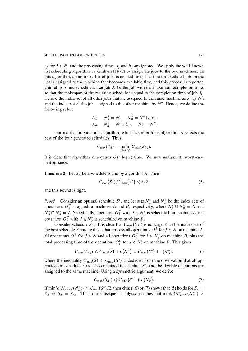
We first specify how the big, medium and small jobs are defined. Let T = a(N) +b(N) + c(N). From theorem 1, T is an upper bound on the makespan for any busyschedule. Consider an arbitrary ε, where 0 < ε < 1. We define ε = ε/4 and introducethe sequence of real numbers δ1, δ2, . . . , where δt = ε2t

.For each integer t , where t � 1, consider the set of jobs

Nt = {Jj | j ∈ N, δ2

t T < max{aj , bj } + cj � δtT}.

Note that the sets of jobs N1, N2, . . . are mutually disjoint. Thus, there exists a τ ∈{1, . . . , 1/ε} such that p(Nτ ) � εT holds; otherwise T � p(N1)+· · ·+p(N 1/ε) >

1/εεT , which is impossible. We define δ = δτ , and note that δ � ε21/ε.

We now partition the jobs into big jobs Wb, medium jobs Wm and small jobs Ws bypartitioning the index set N as follows:

Wb = {j | max{aj , bj } + cj > δT

},

Wm = {j | δ2T < max{aj , bj } + cj � δT

}, (12)

Ws = {j | max{aj , bj } + cj � δ2T

}.

Note that, by definition, Wm = Nτ , which implies

p(Wm) � εT . (13)

3.1. Big jobs

Let nb denote the number of big jobs. From the definition of Wb, each big job has a totalprocessing time that exceeds δT . Since the total processing time of all jobs is equal to T ,we deduce that nb � 1/δ. Moreover, 1/δ � ε−21/ε

, which implies that nb is fixed.We construct 2nb sequences of big jobs as follows. For each j ∈ Wb, we consider

the assignment of the flexible operation OCj to machine A and to machine B. Consid-

ering all big jobs, this produces 2nb possible assignments. For each assignment, we uselemma 1 to produce a sequence of the big jobs.

3.2. Small jobs

Consider any sequence of big jobs as constructed in section 3.1. For notational con-venience, we assume that this sequence begins and ends with a dummy job, where the

SCHEDULING THREE-OPERATION JOBS 181

dummy job has a zero processing time on both machines. Let (J ′0, J

′1, . . . , J

′nb

, J ′nb+1) de-

note this sequence, where J ′0 and J ′

nb+1 are the two dummy jobs. Moreover, let α′k and β ′

k

denote the total processing time of job J ′k on machines A and B, respectively, as specified

by the assignment of the flexible operations of the big jobs, for k = 0, 1, . . . , nb, nb + 1.We now give a procedure based on linear programming that introduces the small jobsinto our sequence.

Let ns denote the number of small jobs. We define variables

xjk =

1 if Jj is scheduled between jobs J ′k−1 and J ′

k,and OC

j is assigned to machine A,0 otherwise;

yjk =

1 if Jj is scheduled between jobs J ′k−1 and J ′

k,and OC

j is assigned to machine B,0 otherwise,

for j ∈ Ws and k = 1, . . . , nb + 1. The following integer program is a relaxation of theproblem of minimizing the makespan for the big and small jobs, where Cmax is a variablethat provides a lower bound on the makespan by considering the big jobs in (1).

Minimize Cmax

subject tou∑

k=1

(∑j∈Ws

((aj + cj )xjk + ajyjk

) + α′k

)+ β ′

u

+nb+1∑

k=u+1

( ∑j∈Ws

(bjxjk + (bj + cj )yjk

) + β ′k

)� Cmax

(u = 0, 1, . . . , nb + 1), (14)nb+1∑k=1

(xjk + yjk) = 1 (j ∈ Ws), (15)

xjk ∈ {0, 1}, yjk ∈ {0, 1} (j ∈ Ws, k = 1, . . . , nb + 1). (16)

Constraints (14) provide upper bounds on the makespan using equation (1). The factthat each small job must be sequenced between some pair of big jobs, either with opera-tion OC

j on machine A or on machine B, is encapsulated in constraints (15).We solve the linear programming relaxation of this problem in which the con-

straints xjk ∈ {0, 1} and yjk ∈ {0, 1} in (16) are replaced by non-negativity constraintsxjk � 0 and yjk � 0. Any small job Jj for which xjk �= 1 and yjk �= 1 for any position k

in this solution is called a fractional job. Note that there are ns + nb + 2 constraints, andconsequently ns +nb+2 basic variables, including Cmax which must be basic. Moreover,each of the ns assignment constraints (15), which ensures that the corresponding smalljob is assigned to a position, contains a distinct set of variables. Following the same typeof analysis as that of Potts (1985), we establish that there are at most nb + 1 fractionaljobs. Each non-fractional small job Jj with xjk = 1 is assigned to a position between

182 GUPTA ET AL.

jobs J ′k−1 and J ′

k, where its flexible operation is assigned to machine A. Similarly, a non-fractional small job Jj with yjk = 1 is assigned to a position between jobs J ′

k−1 and J ′k,

where its flexible operation OCj is assigned to machine B. The small jobs assigned to

positions between jobs J ′k−1 and J ′

k are sequenced using lemma 1, for k = 1, . . . , nb +1.To summarize, the values of the variables for each non-fractional job define the

assignment of its flexible operation and its position relative to the big jobs. On the otherhand, the fractional jobs remain unscheduled at this stage.

3.3. Specifying the approximation scheme

We now present full details of our approximation scheme. Having partitioned the jobsinto subsets containing big, medium and small jobs, we start by considering each pos-sible assignment of the flexible operations of the big jobs. For each assignment, weconstruct a schedule Sε as follows. First, the processing times α′

j and β ′j on machines

A and B of each big job Jj for j ∈ Wb are computed as specified in lemma 1, and thecorresponding sequence of big jobs is obtained by applying Johnson’s algorithm (John-son, 1954) to the processing times α′

j and β ′j for Jj ∈ Wb. The linear programming

relaxation of the problem of assigning small jobs to positions between big jobs that isgiven in section 3.2 is then solved. For each variable xjk = 1, the flexible operation ofjob Jj is assigned to machine A and small job Jj is sequenced between jobs J ′

k−1 and J ′k.

Similarly, yjk = 1 defines the flexible operation of job Jj to be assigned to machine B

and small job Jj is sequenced between J ′k−1 and J ′

k. All small jobs between the big jobsJ ′

k−1 and J ′k are sequenced according to lemma 1, for k = 1, . . . , nb + 1. Finally, any

small job Jj for which there is a variable xjk or yjk that takes a fractional value, thecorresponding small job is appended to the sequence of big and small jobs (after dummyjob J ′

nb+1), where both the assignment of the flexible operation and the order of these ap-pended small jobs is arbitrary. Also, all medium jobs are also appended to this sequencein an arbitrary order, again with an arbitrary assignment of their flexible operations.

3.4. Analysis of the approximation scheme

Let Ws1, . . . ,Ws,nb+1,Ws,nb+2 denote a partition of Ws , where Wsk denotes the set ofsmall jobs that are assigned to positions between jobs J ′

k−1 and J ′k for k = 1, . . . , nb +1,

and Ws,nb+2 denotes the set of fractional small jobs that are sequenced after dummy jobJ ′

nb+1. Thus, schedule Sε is obtained from a sequence

(J ′

0,Ws1, J′1,Ws2, . . . , J

′nb

,Ws,nb+1, J′nb+1,Ws,nb+2,Wm

),

where the ordering of jobs in the different sets is defined in section 3.3. Throughoutthe analysis in this section, we assume that in Sε the flexible operations of big jobs areassigned optimally to machines A and B, as is the case in at least one of the schedules

SCHEDULING THREE-OPERATION JOBS 183

that we consider. Since our construction that derives schedule Sε is obtained from arelaxation of an integer program, we use (14) to deduce that

Cmax(S∗) �

u∑k=1

(α(Wsk) + α′

k

) +nb∑

k=u

(β ′

k + β(Ws,k+1))

(17)

for u = 0, 1, . . . , nb + 1.We use lemma 2 to compute the makespan of schedule Sε. Specifically, we analyze

the cases that a big job J ′u for u = 1, . . . , nb is critical (the dummy jobs cannot be

critical), that a small job in set Wsu for u = 1, . . . , nb + 1 is critical, and that a job inWs,nb+2 or Wm is critical.

First, in the case that a big job J ′u is critical, for u = 1, . . . , nb, we have that

Cmax(Sε) = L(J ′u, Sε), and using (1) we obtain

Cmax(Sε) =u∑

k=1

(α(Wsk) + α′

k

) +nb∑

k=u

(β ′

k + β(Ws,k+1)) + β(Ws,nb+2) + β(Wm)

� Cmax(S∗) + β(Ws,nb+2) + β(Wm), (18)

where the inequality is obtained by substituting (17).Second, in the case that a small job Jj ∈ Wsu is critical, for u = 1, . . . , nb + 1, we

have that Cmax(Sε) = L(Jj , Sε) and using (1) we obtain

Cmax(Sε) =u−1∑k=1

(α(Wsk) + α′

k

) + L(Jj , Sε(Wsu)

)

+nb∑

k=u

(β ′

k + β(Ws,k+1)) + β(Ws,nb+2) + β(Wm), (19)

where L(Jj , Sε(Wsu)) is defined analogously to (1) but only considers jobs of set Wsu inschedule Sε. Thus,

L(Jj , Sε(Wsu)

) =∑i∈Q

αi + αj + βj +∑i∈R

βi,

where Q comprises those jobs in Wsu that are sequenced before Jj and R comprisesthose jobs in Wsu that are sequenced after Jj . If αj � βj , then the ordering of the jobsof Wsu obtained from lemma 1 by the algorithm of Johnson (1954) shows that αi � βi

for i ∈ Q. In this case, L(Jj , Sε(Wsu)) � αj + βj + β(Wsu), and substituting in (19)and applying (17) yields

Cmax(Sε) � Cmax(S∗) + β(Ws,nb+2) + β(Wm) + αj + βj . (20)

Alternatively, if αj > βj , then a similar type of argument shows that αi > βi for i ∈ R,and therefore L(Jj , Sε(Wsu)) � αj +βj +α(Wsu). Thus, using (19) and (17) we deducethat (20) also holds for αj > βj .

184 GUPTA ET AL.

Third, in the case that a job Jj is critical, for Jj ∈ Ws,nb+2 or Jj ∈ Wm, Cmax(Sε) =L(Jj , Sε) and using (1) we obtain

Cmax(Sε) �nb+1∑k=1

(α(Wsk) + α′

k

) + p(Ws,nb+2) + p(Wm)

� Cmax(S∗) + p(Ws,nb+2) + p(Wm), (21)

where p(Ws,nb+2)+p(Wm) is used as an upper bound on the value of L(Jj , Sε(Ws,nb+2 ∪Wm)) in the first inequality, and (17) is used to obtain the second inequality.

From (18), (20) and (21), the makespan for schedule Sε is given by

Cmax(Sε) � Cmax(S∗) + αj + βj + p(Ws,nb+2) + p(Wm), (22)

which is obtained by substituting β(Ws,nb+2) � p(Ws,nb+2) and β(Wm) � p(Wm), whereJj is a small job. As derived in section 3.2, set Ws,nb+2 contains at most nb + 1 smalljobs, so we use (12) to deduce that p(Ws,nb+2) + αj + βj � (2nb + 4)δ2T . Substitutingin (22) and using (13), we obtain

Cmax(Sε) � Cmax(S∗) + (2nb + 4)δ2T + εT . (23)

As shown in section 3.1, nb � 1/δ and 1/δ � ε−21/ε. Thus, since ε < 1/4 we obtain

(2nb + 4)δ2 < ε. Substituting in (23) yields

Cmax(Sε) � Cmax(S∗) + 2εT � (1 + ε)Cmax

(S∗), (24)

where the final inequality is obtained from (2) and our choice ε = ε/4.We now provide the main result in this section.

Theorem 3. The family of approximation algorithms defined in section 3 is a polyno-mial time approximation scheme.

Proof. Inequality (24) establishes that some schedule Sε that is generated by the algo-rithm provides a makespan that is no more than 1+ε times the optimal makespan. Thus,it remains to show that the algorithm requires polynomial time.

The algorithm constructs at most 2nb schedules, one for each possible assignmentof the flexible operations of the big jobs. As shown in section 3.1, this number ofschedules is fixed. For each schedule, a linear programming problem is solved with2ns(nb + 1) + 1 variables and ns + nb + 2 constraints. Such a linear program is solvablein polynomial time, using the algorithm of Vaidya (1989) for example. To obtain the fi-nal schedule from the solution of the linear program, the small jobs are sequenced usingJohnson’s algorithm (Johnson, 1954) in O(ns log ns) time. This establishes that the runtime of the algorithm is polynomial. �

SCHEDULING THREE-OPERATION JOBS 185

4. Concluding remarks

This paper considers a new variant of the classical problem of scheduling jobs in a two-machine flow shop to minimize the makespan. In our problem, each job has three opera-tions, where the middle operation is flexible in that it can be assigned to either the first orthe second machine. Two practical algorithms are analyzed. Specifically, an algorithmwhich uses arbitrary assignment of the flexible operations and an arbitrary processingorder has a worst-case performance ratio of 2. An improved algorithm that constructsfour schedules and selects the best has a worst-case performance ratio of 3/2. Our mainresult shows that the problem has a polynomial time approximation scheme.

The problem is shown to be NP-hard in the ordinary sense, and is conjectured tobe strongly NP-hard. Proving this conjecture is a topic for future research. Anotherinteresting research topic is the development of branch and bound algorithms for findingexact solutions. Finally, it would also be of interest to extend some of the results in thispaper to flow shops with more than two stages.

Acknowledgments

The authors are grateful to Shanling Li of the Faculty of Management at McGill Univer-sity, Montreal, Canada, for bringing this problem to their attention and initial discussionsabout the importance of this problem in industry, and to Emmanuel Néron of the Schoolof Engineering and Informatics for Industry, University of Tours, France, for explainingthe farming application. The comments of anonymous referees have helped improve thepresentation of our work.

References

Garey, M.R. and D.S. Johnson. (1979). Computers and Intractability: A Guide to the Theory of NP-Completeness. New York: Freeman.

Graham, R.L. (1972). “Bounds on Multiprocessing Timing Anomalies.” SIAM Journal of Applied Mathe-matics 17, 416–429.

Graham, R.L., E.L. Lawler, J.K. Lenstra, and A.H.G. Rinnooy Kan. (1979). “Optimization and Approx-imation in Deterministic Sequencing and Scheduling: A Survey.” Annals of Discrete Mathematics 5,287–326.

Hall, L.A. (1998). “Approximability of Flow Shop Scheduling.” Mathematical Programming 82, 175–190.Johnson, S.M. (1954). “Optimal Two- and Three-Stage Production Schedules with Setup Times Included.”

Naval Research Logistics Quarterly 1, 61–68.Néron, E., F. Tercinet, and A. Eloundou. (2000). “Scheduling Identical Jobs on Uniform and Multi-Purpose

Machines.” INFORMS, San Antonio.Potts, C.N. (1985). “Analysis of a Linear Programming Heuristic for Scheduling Unrelated Parallel Ma-

chines.” Discrete Applied Mathematics 10, 155–164.Sevastianov, S.V. and G.J. Woeginger. (1998). “Minimizing Makespan in Open Shops: A Polynomial Time

Approximation Scheme.” Mathematical Programming 82, 191–198.Tanaev, V.S., Y.N. Sotskov, and V.A. Strusevich. (1994). Scheduling Theory. Multi-Stage Systems. Dor-

drecht: Kluwer Academic.Vaidya, P.M. (1989). “Speeding Up Linear Programming using Fast Matrix Multiplication.” In Proceedings

of IEEE 30th Annual Symposium on Foundations of Computer Science, pp. 332–337.