Scheduling to minimize the total compression and late costs

Scheduling To Minimize the Total Compressionand Late Costs

T.C.E. Cheng,1 Zhi-Long Chen,2 Chung-Lun Li,3 B.M.-T. Lin4

1 Office of the Vice President (Research and Postgraduate Studies) , The Hong KongPolytechnic University, Kowloon, Hong Kong, China

2 Department of Systems Engineering, University of Pennsylvania, Philadelphia,Pennsylvania 19104

3 John M. Olin School of Business, Washington University, St. Louis, Missouri 63130

4 Department of Information Management, Ming-Chuan University, Taipei 11120,Taiwan, Republic of China

Received July 1996; revised March 1997; accepted 11 July 1997

Abstract: We consider a single-machine scheduling model in which the job processingtimes are controllable variables with linear costs. The objective is to minimize the sum ofthe cost incurred in compressing job processing times and the cost associated with thenumber of late jobs. The problem is shown to be NP-hard even when the due dates of alljobs are identical. We present a dynamic programming solution algorithm and a fullypolynomial approximation scheme for the problem. Several efficient heuristics are proposedfor solving the problem. Computational experiments demonstrate that the heuristics arecapable of producing near-optimal solutions quickly. q 1998 John Wiley & Sons, Inc. NavalResearch Logistics 45: 67–82, 1998

Keywords: scheduling; sequencing; computational complexity; dynamic programming;approximation schemes

1. INTRODUCTION

Most machine scheduling research has treated job processing times as fixed parameters.In many practical situations, however, the job processing times may be compressed (i.e.,shortened) up to a certain limit through the consumption of additional resources, whichwill result in a higher cost of processing the jobs. But the compression of all or some ofthe job processing times is desirable if it will produce an improved outcome.

Work on machine scheduling problems with controllable job processing times was initi-ated by Vickson [11, 12]. Van Wassenhove and Baker [10], Nowicki and Zdrzalka [7] ,and Panwalkar and Rajagopalan [9] have also made notable contributions to this topic. For

Correspondence to: C.-L. Li

q 1998 by John Wiley & Sons, Inc. CCC 0894-069X/98/010067-16

958/ 8m1b$$0958 12-05-97 18:33:04 nra W: Nav Res

68 Naval Research Logistics, Vol. 45 (1998)

a good summary of the known results for this class of problems, the reader is referred tothe recent survey paper by Nowicki and Zdrzalka [8] .

Daniels and Sarin [3] considered a single-machine scheduling problem in which the jobprocessing times are controllable through the allocation of a limited resource. They providedtheoretical results for constructing the trade-off curve between the number of late jobs andthe total amount of allocated resource. Cheng, Chen, and Li [2] extended Daniels andSarin’s work [3] by resolving the computational complexity issue of the problem andpresented a dynamic programming algorithm for constructing the trade-off curve. The single-machine scheduling problem considered in this paper is similar to the one studied by Danielsand Sarin, except that we wish to minimize the sum of the resource consumption cost ( i.e.,compression cost) and the cost associated with the number of late jobs. Note that, as willbe seen in the ensuing sections, we not only provide in this paper a complexity analysisand a dynamic programming algorithm, but also a fully polynomial approximation schemeand efficient heuristics for our problem.

In our scheduling problem, it is assumed that job preemption is not allowed, all jobs areindependent and simultaneously available at time zero, and the machine can handle onlyone job at a time. Each job has a known normal (maximum) processing time and a knownmaximum possible compression, which is the maximum amount by which the normal jobprocessing time can be compressed. To compress a job will incur a compression costassumed to be linearly varying with the amount of compression. Each job has a known duedate, and a cost will be incurred if a job is late. Thus, there are two types of cost to beconsidered: (1) the compression cost and (2) the cost associated with the number of latejobs. Our objective is to find an optimal job sequence and an optimal processing time foreach job so as to minimize the sum of the compression and late costs.

Note that Chen, Lu, and Tang [1] studied a more general scheduling model where thecompression cost is assumed to be nonlinear with the amount of compression. It may beargued that our problem is a special case of a problem considered in their paper. However,they mainly focused on the complexity issue of the problem, while as mentioned earlierwe will provide in this paper both complexity analysis and solution methods.

For an application of the scheduling problem under study, we may consider the followingscheduling problem arising from the construction industry. The planning office of a smallbuilding contractor sets out to determine the most cost-effective schedule for undertaking anumber of building projects. For each project, the contractor has signed a contract with thedeveloper on which the price, based on the normal project duration, the project due date, andthe late penalty, are spelt out. For any project, it is usually possible to shorten its durationup to a certain extent when necessary. However, to compress the duration of a project, thecontractor will have to employ additional resources, which will increase the construction cost.On the other hand, under certain circumstances, it may be necessary to allow a project toslip past its due date. In this case, the contractor needs to pay the developer the contractualpenalty for late completion. The goal of the planning office is therefore to work out an optimalschedule to carry out the projects at hand such that the total cost of project compression andlate completion is minimized. This scenario is typical of many small contractors which, dueto small size and limited resources, operate on a single-project environment, i.e., the contractorwill pool all its resources to work on only one project at any time.

2. PROBLEM FORMULATION

To facilitate the problem formulation, we introduce the following notation which will beused throughout the paper. It is assumed that all parameters are nonnegative integers. The

958/ 8m1b$$0958 12-05-97 18:33:04 nra W: Nav Res

69Cheng et al.: Scheduling To Minimize Compression and Lateness

integrality assumption should not be a serious limitation, since all the costs and timemeasurements can always be expressed in the smallest unit of measurement for all practicalpurposes. Let

N Å {1, 2, . . . , n} denote the set of jobs to be processed on a machine;aj Å normal (maximum) processing time of job j ;uj Å maximum possible compression of job j(0 ° uj ° aj) ;bj Å minimum processing time of job j (bj Å aj 0 uj) ;xj Å actual compression of job j (0 ° xj ° uj) ;tj Å actual processing time of job j ( tj Å aj 0 xj) ;dj Å due date of job j ;Cj Å completion time of job j ;£j Å unit cost of compressing the processing time of job j ;

wj Å late cost if job j is late, i.e., Cj ú dj;Uj Å 1 if Cj ú dj and 0 otherwise;E Å { j √ NÉCj ° dj} denote the set of early and on-time jobs in a schedule;L Å { j √ NÉCj ú dj} denote the set of late jobs in a schedule;x Å (x1 , x2 , . . . , xn) denote the vector of processing time compressions;

X Å {xÉ0 ° xj ° uj , j √ N} denote the set of all feasible compression vectors;P Å the set of all permutations of N;p Å a permutation of N defining the job sequence, i.e., p √ P.

We note that a pair (x , p) uniquely determines the completion time Cj for each job j √N . This is so because the performance measures considered in this paper are regular, andthus it is not beneficial to insert idle times between jobs. Consequently, each schedule iscompletely defined by the job processing times and a permutation of N . Also note thatsince all parameters are integers, there must exist an optimal solution where all processingtime compressions xi ( i Å 1, . . . , n) are integers.

Two performance measures are considered here. One is the cost associated with thenumber of late jobs, (j√N wjUj ( i.e., the weighted number of late jobs) . The other is thecompression cost, (j√N £j xj . The problem, denoted as (P), can be formulated as follows:

(P) Minimize ∑j√N

wjUj / ∑j√N

£j xj

s.t. x √ X , p √ P.

When £j Å 0 or £j r /` for all j , (P) reduces to 1//( wjUj , which is NP-hard (Karp[5]) , and thus (P) is also NP-hard. When wj Å w and £j Å 0 or £j r /` , (P) reduces to1//( Uj , which is polynomially solvable by Moore’s algorithm (Moore [6]) . We show inSection 4 that (P) is NP-hard even when wj Å w and dj Å d for all j . In Section 3, we givea pseudopolynomial dynamic programming algorithm and a fully polynomial approximationscheme for problem (P). Several heuristics are also designed in Section 5 to obtain near-optimal solutions to the problem.

Before ending this section, we give a basic result which is useful to the analysis in thefollowing sections. We only state the result since its proof is straightforward: For problem(P), there exists an optimal schedule with the following properties:

PROPERTY 1: The set of late jobs are sequenced after the set of early and on-time jobs,

958/ 8m1b$$0958 12-05-97 18:33:04 nra W: Nav Res


i.e., the sequence is in the form (E , L) . Furthermore, the jobs in E are sequenced innondecreasing order of the job due dates, i.e., in the earliest due date (EDD) order, whilethe jobs in L can be in any arbitrary order.

PROPERTY 2: The actual processing time of each late job is equal to its normal pro-cessing time, i.e., xj Å 0 for each j √ L .

3. DYNAMIC PROGRAMMING AND FPAS

In this section we present a pseudopolynomial algorithm and a fully polynomial approxi-mation scheme (FPAS) for a modified version of problem (P). We will treat (P) as amaximization problem which seeks to maximize a total profit function, where ‘‘profit’’ isdefined in such a way that if a job j √ N is completed early or on-time, i.e., Cj ° dj , thenit earns wj 0 £j xj units of profit, where xj is the actual compression of j ; otherwise, it earnsnothing. Let gj denote the profit earned by job j √ N in a given schedule p √ P, i.e.,

gj Å Hwj 0 £j xj , if Cj ° dj ,

0, otherwise.

Then, problem (P) is equivalent to the problem

(P *) Maximize ∑j√N

gj

s.t. x √ X , p √ P.

In order to construct a FPAS for (P*) , we need to make the following assumption:

ASSUMPTION 1: Assume there exist some job k √ N and some integer xk with 0 ° xk

° uk such that dk ¢ ak 0 xk and wk 0 £kxk ú 0.

Assumption 1 means that there is at least one job that can be completed early or on-timeand is profitable if scheduled first. This assumption is made merely to avoid a trivial case.If this assumption does not hold, then in any schedule every job is either late with zeroprofit or early/on-time with a nonpositive profit. This implies that an optimal schedule isobtained by scheduling jobs arbitrarily without any compression and its corresponding totalprofit is zero.

Let

bj Å Hmax{0, wj 0 £j max{0, aj 0 dj}}, if uj ¢ aj 0 dj ,

0, otherwise.

It is easy to see that bj is the maximum possible profit generated by job j in any schedule,i.e., bj is an upper bound on gj in any schedule. Clearly, bj ° wj for all j √ N . ByAssumption 1, there must exist at least one job k with bk ú 0. Thus bmax Å maxj√N{bj}ú 0. On the other hand, it is also easy to see that bj can be realized if job j is scheduled

958/ 8m1b$$0958 12-05-97 18:33:04 nra W: Nav Res


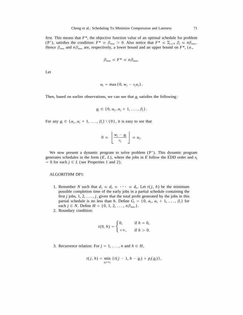
first. This means that F*, the objective function value of an optimal schedule for problem(P *) , satisfies the condition: F* ¢ bmax ú 0. Also notice that F* ° (j√N bj ° nbmax .Hence bmax and nbmax are, respectively, a lower bound and an upper bound on F*, i.e.,

bmax ° F* ° nbmax .

Let

aj Å max{0, wj 0 £juj}.

Then, based on earlier observations, we can see that gj satisfies the following:

gj √ {0, aj , aj / 1, . . . , bj}.

For any gj √ {aj , aj / 1, . . . , bj} " {0}, it is easy to see that

0 ° wj 0 gj

£j

° uj .

We now present a dynamic program to solve problem (P *) . This dynamic programgenerates schedules in the form (E , L) , where the jobs in E follow the EDD order and xj

Å 0 for each j √ L (see Properties 1 and 2).

ALGORITHM DP1:

1. Renumber N such that d1 ° d2 ° rrr ° dn . Let t( j , h) be the minimumpossible completion time of the early jobs in a partial schedule containing thefirst j jobs, 1, 2, . . . , j , given that the total profit generated by the jobs in thispartial schedule is no less than h . Define Gj Å {0, aj , aj / 1, . . . , bj} foreach j √ N . Define H Å {0, 1, 2, . . . , nbmax}.

2. Boundary condition:

t(0, h) Å H0, if h Å 0,

/` , if h ú 0.

3. Recurrence relation: For j Å 1, . . . , n and h √ H ,

t( j , h) Å mingj√Gj

{ t( j 0 1, h 0 gj) / pj( gj)},

958/ 8m1b$$0958 12-05-97 18:33:04 nra W: Nav Res


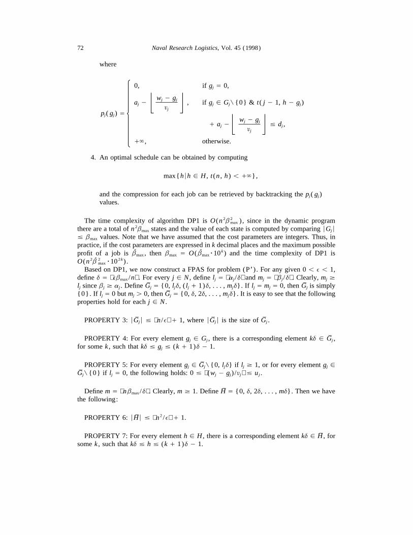
where

pj( gj) Å

0, if gj Å 0,

aj 0wj 0 gj

£j

, if gj √ Gj" {0} & t( j 0 1, h 0 gj)

/ aj 0wj 0 gj

£j

° dj ,

/` , otherwise.

4. An optimal schedule can be obtained by computing

max{hÉh √ H , t(n , h) õ /`},

and the compression for each job can be retrieved by backtracking the pj( gj)values.

The time complexity of algorithm DP1 is O(n 2b 2max ) , since in the dynamic program

there are a total of n 2bmax states and the value of each state is computed by comparing ÉGjÉ

° bmax values. Note that we have assumed that the cost parameters are integers. Thus, inpractice, if the cost parameters are expressed in k decimal places and the maximum possibleprofit of a job is bO max , then bmax Å O(bO maxr10 k) and the time complexity of DP1 isO(n 2bO 2

maxr102k) .Based on DP1, we now construct a FPAS for problem (P*) . For any given 0 õ e õ 1,

define d Å ebmax /n . For every j √ N , define lj Å aj/d and mj Å bj/d . Clearly, mj ¢lj since bj ¢ aj . Define GV j Å {0, ljd, ( lj / 1)d, . . . , mjd}. If lj Å mj Å 0, then GV j is simply{0}. If lj Å 0 but mj ú 0, then GV j Å {0, d, 2d, . . . , mjd}. It is easy to see that the followingproperties hold for each j √ N .

PROPERTY 3: ÉGV jÉ ° n /e / 1, where ÉGV jÉ is the size of GV j .

PROPERTY 4: For every element gj √ Gj , there is a corresponding element kd √ GV j ,for some k , such that kd ° gj ° (k / 1)d 0 1.

PROPERTY 5: For every element gj √ GV j" {0, ljd} if lj ¢ 1, or for every element gj √GV j" {0} if lj Å 0, the following holds: 0 ° (wj 0 gj) /£j ° uj .

Define m Å nbmax /d . Clearly, m ¢ 1. Define HV Å {0, d, 2d, . . . , md}. Then we havethe following:

PROPERTY 6: ÉHV É ° n 2 /e / 1.

PROPERTY 7: For every element h √ H , there is a corresponding element kd √ HV , forsome k , such that kd ° h ° (k / 1)d 0 1.

958/ 8m1b$$0958 12-05-97 18:33:04 nra W: Nav Res


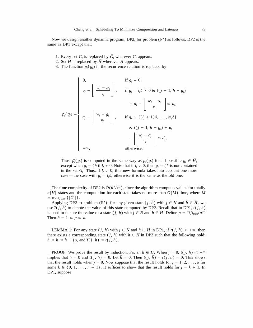
Now we design another dynamic program, DP2, for problem (P *) as follows. DP2 is thesame as DP1 except that:

1. Every set Gj is replaced by GV j wherever Gj appears.2. Set H is replaced by HV wherever H appears.3. The function pj( gj) in the recurrence relation is replaced by

pV j( gj) Å

0, if gj Å 0,

aj 0wj 0 aj

£j

, if gj Å ljd x 0 & t( j 0 1, h 0 gj)

/ aj 0wj 0 aj

£j

° dj ,

aj 0wj 0 gj

£j

, if gj √ {( lj / 1)d, . . . , mjd}

& t( j 0 1, h 0 gj) / aj

0 wj 0 gj

£j

° dj ,

/` , otherwise.

Thus, pV j( gj) is computed in the same way as pj( gj) for all possible gj √ HV ,

except when gj Å ljd if lj x 0. Note that if lj x 0, then gj Å ljd is not containedin the set Gj . Thus, if lj x 0, this new formula takes into account one morecase—the case with gj Å ljd; otherwise it is the same as the old one.

The time complexity of DP2 is O(n 4 /e 2) , since the algorithm computes values for totallynÉHV É states and the computation for each state takes no more than O(M) time, where MÅ maxj√N {ÉGV jÉ}.

Applying DP2 to problem (P *) , for any given state ( j , hU ) with j √ N and hU √ HV , weuse t

U( j , hU ) to denote the value of this state computed by DP2. Recall that in DP1, t( j , h)

is used to denote the value of a state ( j , h) with j √ N and h √ H . Define r Å ebmax /n .Then d 0 1 ° r ° d.

LEMMA 1: For any state ( j , h) with j √ N and h √ H in DP1, if t( j , h) õ /` , thenthere exists a corresponding state ( j , hU ) with hU √ HV in DP2 such that the following hold:hU ° h ° hU / jr, and t

U( j , hU ) ° t( j , h) .

PROOF: We prove the result by induction. Fix an h √ H . When j Å 0, t( j , h) õ /`implies that h Å 0 and t( j , h) Å 0. Let hU Å 0. Then t

U( j , hU ) Å t( j , h) Å 0. This shows

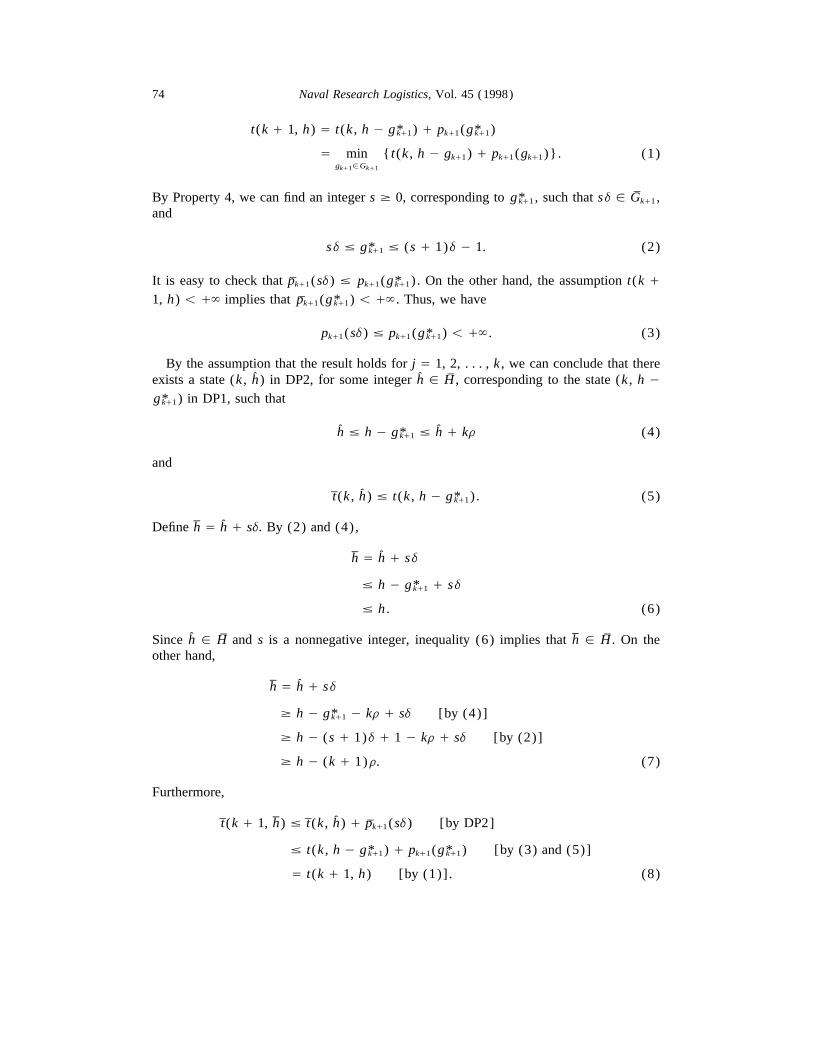
that the result holds when j Å 0. Now suppose that the result holds for j Å 1, 2, . . . , k forsome k √ {0, 1, . . . , n 0 1}. It suffices to show that the result holds for j Å k / 1. InDP1, suppose

958/ 8m1b$$0958 12-05-97 18:33:04 nra W: Nav Res


t(k / 1, h) Å t(k , h 0 g*k/1) / pk/1(g*k/1)

Å mingk/1√Gk/1

{ t(k , h 0 gk/1) / pk/1(gk/1)}. (1)

By Property 4, we can find an integer s ¢ 0, corresponding to g*k/1 , such that sd √ GV k/1 ,and

sd ° g*k/1 ° (s / 1)d 0 1. (2)

It is easy to check that pV k/1(sd) ° pk/1(g*k/1) . On the other hand, the assumption t(k /

1, h) õ /` implies that pV k/1(g*k/1) õ /` . Thus, we have

pk/1(sd) ° pk/1(g*k/1) õ /` . (3)

By the assumption that the result holds for j Å 1, 2, . . . , k , we can conclude that thereexists a state (k , hO ) in DP2, for some integer hO √ HV , corresponding to the state (k , h 0g*k/1) in DP1, such that

hO ° h 0 g*k/1 ° hO / kr (4)

and

tU(k , hO ) ° t(k , h 0 g*k/1) . (5)

Define hU Å hO / sd. By (2) and (4),

hU Å hO / sd

° h 0 g*k/1 / sd

° h . (6)

Since hO √ HV and s is a nonnegative integer, inequality (6) implies that hU √ HV . On theother hand,

hU Å hO / sd

¢ h 0 g*k/1 0 kr / sd [by (4)]

¢ h 0 (s / 1)d / 1 0 kr / sd [by (2)]

¢ h 0 (k / 1)r. (7)

Furthermore,

tU(k / 1, hU ) ° t

U(k , hO ) / p

V k/1(sd) [by DP2]

° t(k , h 0 g*k/1) / pk/1(g*k/1) [by (3) and (5)]

Å t(k / 1, h) [by (1)] . (8)

958/ 8m1b$$0958 12-05-97 18:33:04 nra W: Nav Res


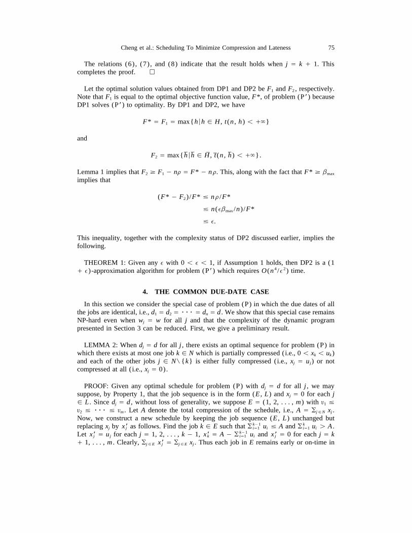
The relations (6) , (7) , and (8) indicate that the result holds when j Å k / 1. Thiscompletes the proof. h

Let the optimal solution values obtained from DP1 and DP2 be F1 and F2 , respectively.Note that F1 is equal to the optimal objective function value, F*, of problem (P*) becauseDP1 solves (P*) to optimality. By DP1 and DP2, we have

F* Å F1 Å max{hÉh √ H , t(n , h) õ /`}

and

F2 Å max{hU ÉhU √ HU , tU(n , hU ) õ /`}.

Lemma 1 implies that F2 ¢ F1 0 nr Å F* 0 nr. This, along with the fact that F* ¢ bmax

implies that

(F* 0 F2) /F* ° nr /F*

° n(ebmax /n) /F*

° e.

This inequality, together with the complexity status of DP2 discussed earlier, implies thefollowing.

THEOREM 1: Given any e with 0 õ e õ 1, if Assumption 1 holds, then DP2 is a (1/ e)-approximation algorithm for problem (P*) which requires O(n 4 /e 2) time.

4. THE COMMON DUE-DATE CASE

In this section we consider the special case of problem (P) in which the due dates of allthe jobs are identical, i.e., d1 Å d2 Å rrr Å dn Å d . We show that this special case remainsNP-hard even when wj Å w for all j and that the complexity of the dynamic programpresented in Section 3 can be reduced. First, we give a preliminary result.

LEMMA 2: When dj Å d for all j , there exists an optimal sequence for problem (P) inwhich there exists at most one job k √ N which is partially compressed (i.e., 0 õ xk õ uk)and each of the other jobs j √ N" {k} is either fully compressed (i.e., xj Å uj) or notcompressed at all ( i.e., xj Å 0).

PROOF: Given any optimal schedule for problem (P) with dj Å d for all j , we maysuppose, by Property 1, that the job sequence is in the form (E , L) and xj Å 0 for each j√ L . Since dj Å d , without loss of generality, we suppose E Å (1, 2, . . . , m) with £1 °£2 ° rrr ° £m . Let A denote the total compression of the schedule, i.e., A Å (j√N xj .Now, we construct a new schedule by keeping the job sequence (E , L) unchanged butreplacing xj by x *j as follows. Find the job k √ E such that ( k01

iÅ1 ui ° A and ( kiÅ1 ui ú A .

Let x *j Å uj for each j Å 1, 2, . . . , k 0 1, x *k Å A 0 ( k01iÅ1 ui and x *j Å 0 for each j Å k

/ 1, . . . , m . Clearly, (j√E x *j Å (j√E xj . Thus each job in E remains early or on-time in

958/ 8m1b$$0958 12-05-97 18:33:04 nra W: Nav Res


the new schedule. Also, the weighted number of late jobs in the new schedule is the sameas that in the original schedule. Since £1 ° £2 ° rrr ° £m , it is easy to see that (j√E

£j x *j ° (j√E £j xj , i.e., the compression cost associated with the new schedule is no greaterthan that associated with the original schedule. Thus, the new schedule is also optimal andthere exists in this schedule at most one job (i.e., job k) which is partially compressed.h

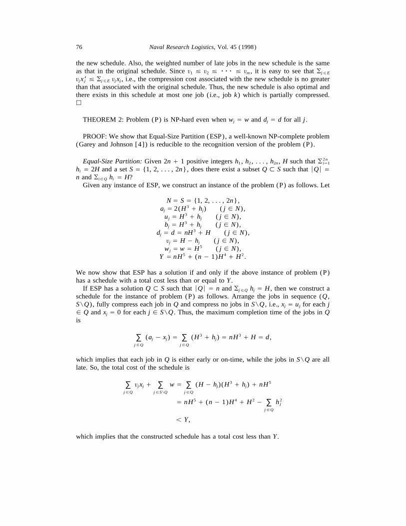
THEOREM 2: Problem (P) is NP-hard even when wj Å w and dj Å d for all j .

PROOF: We show that Equal-Size Partition (ESP), a well-known NP-complete problem(Garey and Johnson [4]) is reducible to the recognition version of the problem (P).

Equal-Size Partition: Given 2n / 1 positive integers h1 , h2 , . . . , h2n , H such that ( 2niÅ1

hi Å 2H and a set S Å {1, 2, . . . , 2n}, does there exist a subset Q , S such that ÉQÉ Ån and (i√Q hi Å H?

Given any instance of ESP, we construct an instance of the problem (P) as follows. Let

N Å S Å {1, 2, . . . , 2n},aj Å 2(H 3 / hj) ( j √ N) ,

uj Å H 3 / hj ( j √ N) ,bj Å H 3 / hj ( j √ N) ,

dj Å d Å nH 3 / H ( j √ N) ,£j Å H 0 hj ( j √ N) ,

wj Å w Å H 5 ( j √ N) ,Y Å nH 5 / (n 0 1)H 4 / H 2 .

We now show that ESP has a solution if and only if the above instance of problem (P)has a schedule with a total cost less than or equal to Y .

If ESP has a solution Q , S such that ÉQÉ Å n and (j√Q hj Å H , then we construct aschedule for the instance of problem (P) as follows. Arrange the jobs in sequence (Q ,S"Q) , fully compress each job in Q and compress no jobs in S"Q , i.e., xj Å uj for each j√ Q and xj Å 0 for each j √ S"Q . Thus, the maximum completion time of the jobs in Qis

∑j√Q

(aj 0 xj) Å ∑j√Q

(H 3 / hj) Å nH 3 / H Å d ,

which implies that each job in Q is either early or on-time, while the jobs in S"Q are alllate. So, the total cost of the schedule is

∑j√Q

£j xj / ∑j√S"Q

w Å ∑j√Q

(H 0 hj)(H 3 / hj) / nH 5

Å nH 5 / (n 0 1)H 4 / H 2 0 ∑j√Q

h 2j

õ Y ,

which implies that the constructed schedule has a total cost less than Y .

958/ 8m1b$$0958 12-05-97 18:33:04 nra W: Nav Res


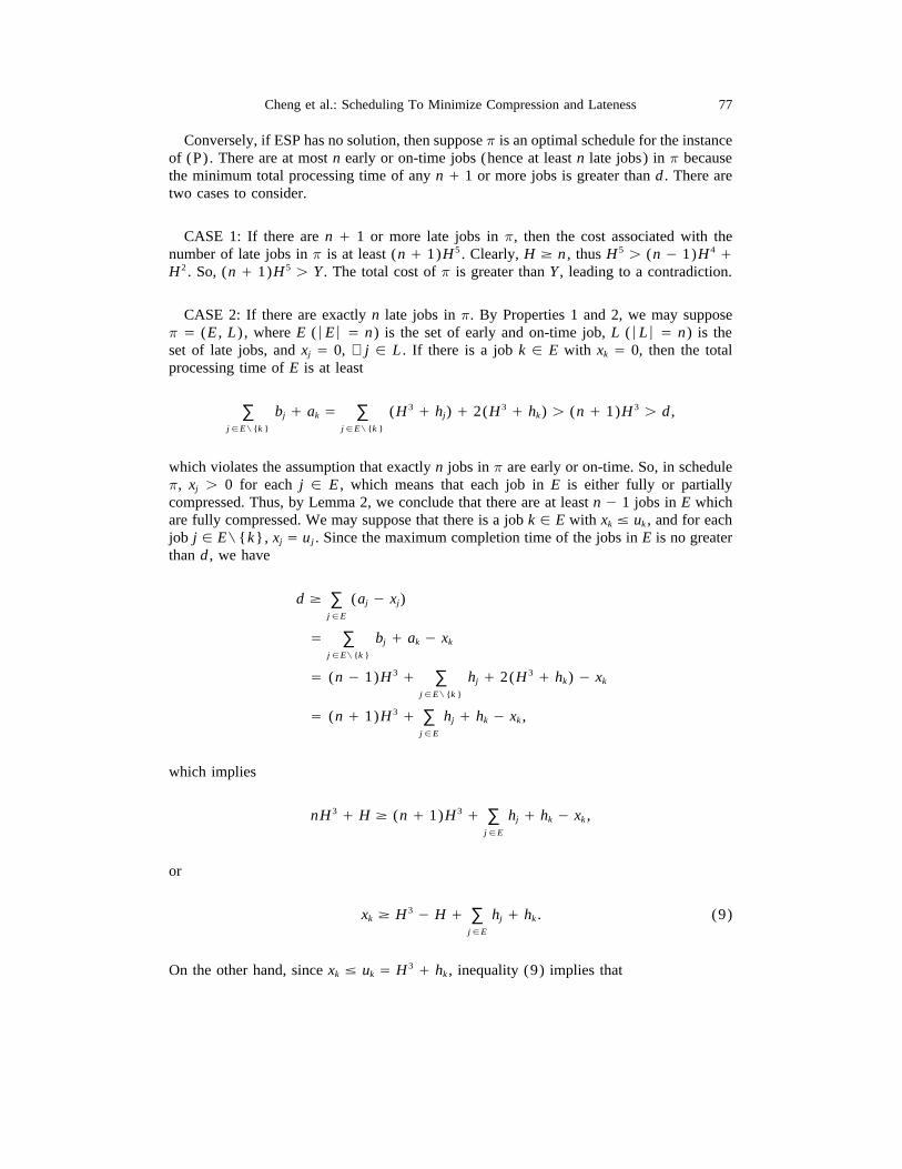
Conversely, if ESP has no solution, then suppose p is an optimal schedule for the instanceof (P). There are at most n early or on-time jobs (hence at least n late jobs) in p becausethe minimum total processing time of any n / 1 or more jobs is greater than d . There aretwo cases to consider.

CASE 1: If there are n / 1 or more late jobs in p, then the cost associated with thenumber of late jobs in p is at least (n / 1)H 5 . Clearly, H ¢ n , thus H 5 ú (n 0 1)H 4 /H 2 . So, (n / 1)H 5 ú Y . The total cost of p is greater than Y , leading to a contradiction.

CASE 2: If there are exactly n late jobs in p. By Properties 1 and 2, we may supposep Å (E , L) , where E (ÉEÉ Å n) is the set of early and on-time job, L (ÉLÉ Å n) is theset of late jobs, and xj Å 0, ∀ j √ L . If there is a job k √ E with xk Å 0, then the totalprocessing time of E is at least

∑j√E" {k }

bj / ak Å ∑j√E" {k }

(H 3 / hj) / 2(H 3 / hk) ú (n / 1)H 3 ú d ,

which violates the assumption that exactly n jobs in p are early or on-time. So, in schedulep, xj ú 0 for each j √ E , which means that each job in E is either fully or partiallycompressed. Thus, by Lemma 2, we conclude that there are at least n 0 1 jobs in E whichare fully compressed. We may suppose that there is a job k √ E with xk ° uk , and for eachjob j √ E" {k}, xj Å uj . Since the maximum completion time of the jobs in E is no greaterthan d , we have

d ¢ ∑j√E

(aj 0 xj)

Å ∑j√E" {k }

bj / ak 0 xk

Å (n 0 1)H 3 / ∑j√E" {k }

hj / 2(H 3 / hk) 0 xk

Å (n / 1)H 3 / ∑j√E

hj / hk 0 xk ,

which implies

nH 3 / H ¢ (n / 1)H 3 / ∑j√E

hj / hk 0 xk ,

or

xk ¢ H 3 0 H / ∑j√E

hj / hk . (9)

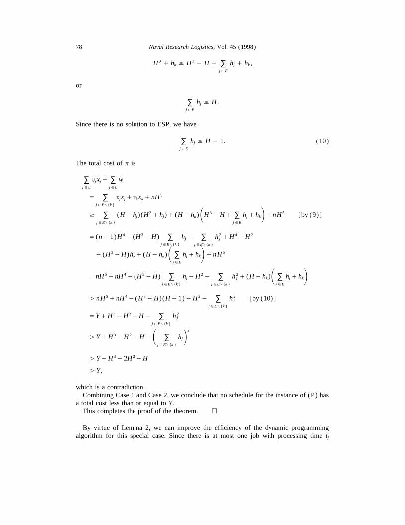
On the other hand, since xk ° uk Å H 3 / hk , inequality (9) implies that

958/ 8m1b$$0958 12-05-97 18:33:04 nra W: Nav Res


H 3 / hk ¢ H 3 0 H / ∑j√E

hj / hk ,

or

∑j√E

hj ° H .

Since there is no solution to ESP, we have

∑j√E

hj ° H 0 1. (10)

The total cost of p is

∑j√E

£j xj/ ∑j√L

w

Å ∑j√E" {k }

£j xj/ £kxk/ nH 5

¢ ∑j√E" {k }

(H0 hj)(H 3/ hj)/ (H0 hk)SH 30H/ ∑j√E

hj/ hkD/ nH 5 [by (9)]

Å (n0 1)H 40 (H 30H) ∑j√E" {k }

hj0 ∑j√E" {k }

h 2j /H 40H 2

0 (H 30H)hk/ (H0 hk)S ∑j√E

hj/ hkD/ nH 5

Å nH 5/ nH 40 (H 30H) ∑j√E" {k }

hj0H 20 ∑j√E" {k }

h 2j / (H0 hk)S ∑

j√E

hj/ hkDú nH 5/ nH 40 (H 30H)(H0 1)0H 20 ∑

j√E" {k }

h 2j [by (10)]

Å Y/H 30H 20H0 ∑j√E" {k }

h 2j

ú Y/H 30H 20H0 S ∑j√E" {k }

hjD2

ú Y/H 30 2H 20H

ú Y ,

which is a contradiction.Combining Case 1 and Case 2, we conclude that no schedule for the instance of (P) has

a total cost less than or equal to Y .This completes the proof of the theorem. h

By virtue of Lemma 2, we can improve the efficiency of the dynamic programmingalgorithm for this special case. Since there is at most one job with processing time tj

958/ 8m1b$$0958 12-05-97 18:33:04 nra W: Nav Res


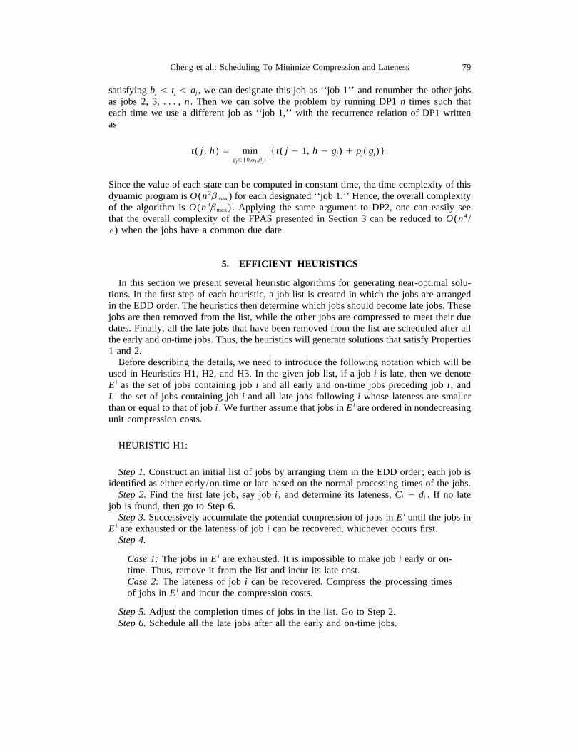
satisfying bj õ tj õ aj , we can designate this job as ‘‘job 1’’ and renumber the other jobsas jobs 2, 3, . . . , n . Then we can solve the problem by running DP1 n times such thateach time we use a different job as ‘‘job 1,’’ with the recurrence relation of DP1 writtenas

t( j , h) Å mingj√{0,aj ,bj}

{ t( j 0 1, h 0 gj) / pj( gj)}.

Since the value of each state can be computed in constant time, the time complexity of thisdynamic program is O(n 2bmax) for each designated ‘‘job 1.’’ Hence, the overall complexityof the algorithm is O(n 3bmax) . Applying the same argument to DP2, one can easily seethat the overall complexity of the FPAS presented in Section 3 can be reduced to O(n 4 /e) when the jobs have a common due date.

5. EFFICIENT HEURISTICS

In this section we present several heuristic algorithms for generating near-optimal solu-tions. In the first step of each heuristic, a job list is created in which the jobs are arrangedin the EDD order. The heuristics then determine which jobs should become late jobs. Thesejobs are then removed from the list, while the other jobs are compressed to meet their duedates. Finally, all the late jobs that have been removed from the list are scheduled after allthe early and on-time jobs. Thus, the heuristics will generate solutions that satisfy Properties1 and 2.

Before describing the details, we need to introduce the following notation which will beused in Heuristics H1, H2, and H3. In the given job list, if a job i is late, then we denoteEi as the set of jobs containing job i and all early and on-time jobs preceding job i , andLi the set of jobs containing job i and all late jobs following i whose lateness are smallerthan or equal to that of job i . We further assume that jobs in Ei are ordered in nondecreasingunit compression costs.

HEURISTIC H1:

Step 1. Construct an initial list of jobs by arranging them in the EDD order; each job isidentified as either early/on-time or late based on the normal processing times of the jobs.

Step 2. Find the first late job, say job i , and determine its lateness, Ci 0 di . If no latejob is found, then go to Step 6.

Step 3. Successively accumulate the potential compression of jobs in Ei until the jobs inEi are exhausted or the lateness of job i can be recovered, whichever occurs first.

Step 4.

Case 1: The jobs in Ei are exhausted. It is impossible to make job i early or on-time. Thus, remove it from the list and incur its late cost.Case 2: The lateness of job i can be recovered. Compress the processing timesof jobs in Ei and incur the compression costs.

Step 5. Adjust the completion times of jobs in the list. Go to Step 2.Step 6. Schedule all the late jobs after all the early and on-time jobs.

958/ 8m1b$$0958 12-05-97 18:33:04 nra W: Nav Res


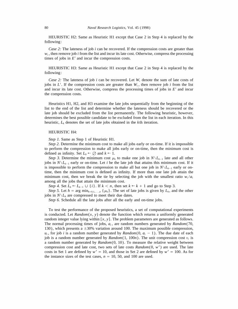
HEURISTIC H2: Same as Heuristic H1 except that Case 2 in Step 4 is replaced by thefollowing:

Case 2: The lateness of job i can be recovered. If the compression costs are greater thanwi , then remove job i from the list and incur its late cost. Otherwise, compress the processingtimes of jobs in Ei and incur the compression costs.

HEURISTIC H3: Same as Heuristic H1 except that Case 2 in Step 4 is replaced by thefollowing:

Case 2: The lateness of job i can be recovered. Let Wi denote the sum of late costs ofjobs in Li . If the compression costs are greater than Wi , then remove job i from the listand incur its late cost. Otherwise, compress the processing times of jobs in Ei and incurthe compression costs.

Heuristics H1, H2, and H3 examine the late jobs sequentially from the beginning of thelist to the end of the list and determine whether the lateness should be recovered or thelate job should be excluded from the list permanently. The following heuristic, however,determines the best possible candidate to be excluded from the list in each iteration. In thisheuristic, Lk denotes the set of late jobs obtained in the k th iteration.

HEURISTIC H4:

Step 1. Same as Step 1 of Heuristic H1.Step 2. Determine the minimum cost to make all jobs early or on-time. If it is impossible

to perform the compression to make all jobs early or on-time, then the minimum cost isdefined as infinity. Set L0 R M and k R 1.

Step 3. Determine the minimum cost mk to make one job in N"Lk01 late and all otherjobs in N"Lk01 early or on-time. Let i be the late job that attains this minimum cost. If itis impossible to perform the compression to make all but one job in N"Lk01 early or on-time, then the minimum cost is defined as infinity. If more than one late job attain theminimum cost, then we break the tie by selecting the job with the smallest ratio wi /ai

among all the jobs that attain the minimum cost.Step 4. Set Lk R Lk01 < { i}. If k õ n , then set k R k / 1 and go to Step 3.Step 5. Let h Å arg minkÅ0,1,. . . ,n {mk}. The set of late jobs is given by Lh , and the other

jobs in N"Lh are compressed to meet their due dates.Step 6. Schedule all the late jobs after all the early and on-time jobs.

To test the performance of the proposed heuristics, a set of computational experimentsis conducted. Let Random(x , y) denote the function which returns a uniformly generatedrandom integer value lying within [x , y] . The problem parameters are generated as follows.The normal processing times of jobs, ai , are random numbers generated by Random(70,130), which presents a {30% variation around 100. The maximum possible compression,ui , for job i is a random number generated by Random(0, ai 0 1). The due date of eachjob is a random number generated by Random(1, 100n) . The unit compression cost £i isa random number generated by Random(0, 10). To measure the relative weight betweencompression cost and late cost, two sets of late costs Random(0, w *) are used. The latecosts in Set 1 are defined by w * Å 10, and those in Set 2 are defined by w * Å 100. As forthe instance sizes of the test cases, n Å 10, 50, and 100 are used.

958/ 8m1b$$0958 12-05-97 18:33:04 nra W: Nav Res


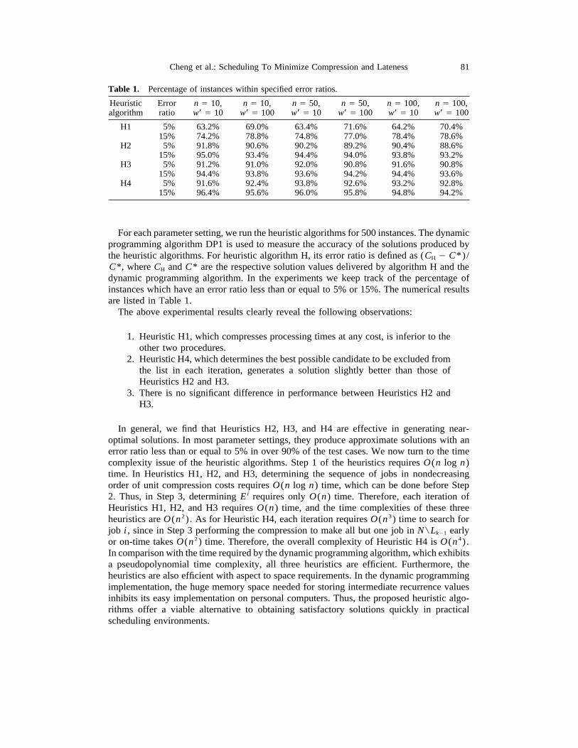
Table 1. Percentage of instances within specified error ratios.

Heuristic Error n Å 10, n Å 10, n Å 50, n Å 50, n Å 100, n Å 100,algorithm ratio w* Å 10 w* Å 100 w* Å 10 w* Å 100 w* Å 10 w* Å 100

H1 5% 63.2% 69.0% 63.4% 71.6% 64.2% 70.4%15% 74.2% 78.8% 74.8% 77.0% 78.4% 78.6%

H2 5% 91.8% 90.6% 90.2% 89.2% 90.4% 88.6%15% 95.0% 93.4% 94.4% 94.0% 93.8% 93.2%

H3 5% 91.2% 91.0% 92.0% 90.8% 91.6% 90.8%15% 94.4% 93.8% 93.6% 94.2% 94.4% 93.6%

H4 5% 91.6% 92.4% 93.8% 92.6% 93.2% 92.8%15% 96.4% 95.6% 96.0% 95.8% 94.8% 94.2%

For each parameter setting, we run the heuristic algorithms for 500 instances. The dynamicprogramming algorithm DP1 is used to measure the accuracy of the solutions produced bythe heuristic algorithms. For heuristic algorithm H, its error ratio is defined as (CH 0 C*)/C*, where CH and C* are the respective solution values delivered by algorithm H and thedynamic programming algorithm. In the experiments we keep track of the percentage ofinstances which have an error ratio less than or equal to 5% or 15%. The numerical resultsare listed in Table 1.

The above experimental results clearly reveal the following observations:

1. Heuristic H1, which compresses processing times at any cost, is inferior to theother two procedures.

2. Heuristic H4, which determines the best possible candidate to be excluded fromthe list in each iteration, generates a solution slightly better than those ofHeuristics H2 and H3.

3. There is no significant difference in performance between Heuristics H2 andH3.

In general, we find that Heuristics H2, H3, and H4 are effective in generating near-optimal solutions. In most parameter settings, they produce approximate solutions with anerror ratio less than or equal to 5% in over 90% of the test cases. We now turn to the timecomplexity issue of the heuristic algorithms. Step 1 of the heuristics requires O(n log n)time. In Heuristics H1, H2, and H3, determining the sequence of jobs in nondecreasingorder of unit compression costs requires O(n log n) time, which can be done before Step2. Thus, in Step 3, determining Ei requires only O(n) time. Therefore, each iteration ofHeuristics H1, H2, and H3 requires O(n) time, and the time complexities of these threeheuristics are O(n 2) . As for Heuristic H4, each iteration requires O(n 3) time to search forjob i , since in Step 3 performing the compression to make all but one job in N"Lk01 earlyor on-time takes O(n 2) time. Therefore, the overall complexity of Heuristic H4 is O(n 4) .In comparison with the time required by the dynamic programming algorithm, which exhibitsa pseudopolynomial time complexity, all three heuristics are efficient. Furthermore, theheuristics are also efficient with aspect to space requirements. In the dynamic programmingimplementation, the huge memory space needed for storing intermediate recurrence valuesinhibits its easy implementation on personal computers. Thus, the proposed heuristic algo-rithms offer a viable alternative to obtaining satisfactory solutions quickly in practicalscheduling environments.

958/ 8m1b$$0958 12-05-97 18:33:04 nra W: Nav Res


6. CONCLUSIONS

We have considered in this paper a problem arising from a single-machine schedulingmodel involving controllable processing times and weighted number of late jobs. Theproblem is NP-hard even when all the jobs have a common due date and the same latenesscost. We have presented a pseudopolynomial dynamic programming algorithm, as well asa fully polynomial approximation scheme, for solving the problem. The efficiency of thedynamic program can be improved when all due dates are identical. Some heuristics havebeen proposed, and the computational results have shown that the heuristics are capable ofproducing near-optimal solutions quickly.

ACKNOWLEDGMENTS

The authors would like to thank two anonymous referees for their helpful suggestionsand comments on an earlier version of this paper.

REFERENCES

[1] Chen, Z.-L., Lu, Q., and Tang, G., ‘‘Single Machine Scheduling with Discretely ControllableProcessing Times,’’ Operations Research Letters, to appear.

[2] Cheng, T.C.E., Chen, Z.-L., and Li, C.-L., ‘‘Single-Machine Scheduling with Trade-Off betweenNumber of Tardy Jobs and Resource Allocation,’’ Operations Research Letters, 19, 237–242(1996).

[3] Daniels, R.L., and Sarin, R.K., ‘‘Single Machine Scheduling with Controllable Processing Timesand Number of Jobs Tardy,’’ Operations Research, 37, 981–984 (1989).

[4] Garey, M.R., and Johnson, D.S., Computers and Intractability: A Guide to the Theory of NP-Hardness, Freeman, San Francisco, 1979.

[5] Karp, R.M., ‘‘Reducibility Among Combinatorial Algorithms,’’ in R.E. Miller and J.W.Thatcher (Eds.) , Complexity of Computer Computations, Plenum, New York, 1972, pp. 85–103.

[6] Moore, J.M., ‘‘An n Job, One-Machine Sequencing Algorithm for Minimizing the Number ofLate Jobs,’’ Management Science, 15, 334–342 (1968).

[7] Nowicki, E., and Zdrzalka, S., ‘‘A Two-Machine Flow Shop Scheduling Problem with Controlla-ble Job Processing Times,’’ European Journal of Operational Research, 34, 208–220 (1988).

[8] Nowicki, E., and Zdrzalka, S., ‘‘A Survey of Results for Sequencing Problems with ControllableProcessing Times,’’ Discrete Applied Mathematics, 26, 271–287 (1990).

[9] Panwalkar, S.S., and Rajagopalan, R., ‘‘Single-Machine Sequencing with Controllable Pro-cessing Times,’’ European Journal of Operational Research, 59, 298–302 (1992).

[10] Van Wassenhove, L.N., and Baker, K.R., ‘‘A Bicriterion Approach to Time/Cost Trade-Offsin Sequencing,’’ European Journal of Operational Research, 11, 48–54 (1982).

[11] Vickson, R.G., ‘‘Choosing the Job Sequence and Processing Times To Minimize Total Pro-cessing plus Flow Cost on a Single Machine,’’ Operations Research, 28, 1155–1167 (1980).

[12] Vickson, R.G., ‘‘Two Single Machine Sequencing Problems Involving Controllable Job Pro-cessing Times,’’ IIE Transactions, 12, 258–262 (1980).

958/ 8m1b$$0958 12-05-97 18:33:04 nra W: Nav Res

Documents

Scheduling to minimize the total compression and late costs