Embed Size (px)
Citation preview
G. Fotopoulos, C. Kotsakis, M.G. Sideris
Evaluation of Geoid Models and Their Use in Combined GPS/Levelling/Geoid Height Network Adjustments
Report Nr. 1999.4
Universität Stuttgart
Technical Reports Department of Geodesy and Geoinformatics
Schriftenreihe der Institute des Studiengangs Geodäsie und Geoinformatik
ifpifp
Stuttgart
G I
ISSN 0933-2839
Evaluation of Geoid Models and Their Use in
Combined GPS/Levelling/Geoid Height Network
Adjustments
Prepared by:
G. Fotopoulos, C. Kotsakis, and M.G. Sideris
Department of Geomatics Engineering
The University of Calgary
2500 University Drive N.W.
Calgary, Alberta, Canada T2N 1N4
June 1999
i
Table of Contents
Abstract ..............................................................................................................................1
1. Introduction..................................................................................................................2
2. Development of a New Canadian Geoid Model ........................................................4
2.1 Computational Methodology............................................................................5
2.2 GARR98 ...........................................................................................................9
3. Evaluation of Various Geoid Models .......................................................................10
3.1 Comparisons Between Geoid Models ............................................................10
3.2 Comparisons at GPS Benchmarks ..................................................................14
3.3 Absolute Agreement of Geoid Models with Respect to GPS/Levelling ........15
3.4 Relative Agreement of Geoid Models with Respect to GPS/Levelling .........19
3.5 Results from a Kinematic DGPS Campaign...................................................23
4. Adjustment of Combined GPS/Levelling/Geoid Networks....................................25
4.1 Overview of Various Adjustment Schemes....................................................26
4.1.1 Geoid Evaluation................................................................................27
4.1.2 Corrector Surface for GPS/Levelling ......................................................28
4.1.3 Gravimetric Geoid Refinement ..............................................................29
4.1.4 Vertical Datum Testing/Refinement .......................................................29
4.2 General Modelling Considerations .................................................................30
4.3 A General Adjustment Model.........................................................................32
4.4 A Purely Deterministic Approach ..................................................................37
4.5 Some Preliminary Numerical Tests of Methods Used for the Adjustment of
Combined GLG Networks .............................................................................41
4.5.1 Western Canada .................................................................................41
4.5.2 Eastern Canada...................................................................................47
4.5.3 Surface Plots......................................................................................50
4.6 A ’Collocation’ Approach................................................................................52
4.7 Statistical Testing in GPS/Levelling/Geoid Networks ...................................58
5. Concluding Remarks .................................................................................................63
6. Acknowledgements ....................................................................................................65
7. References...................................................................................................................66
1
Abstract
The purpose of this report is to provide a comprehensive evaluation of geoid models and
study their use in combined GPS/levelling/geoid height network adjustments. The
information obtained from combining the three height data sets (ellipsoidal, orthometric
and geoidal heights) is valuable for many applications and can be more efficient and
accurate than traditional techniques. The development of a new gravimetric geoid model
(GARR98) for Canada and parts of the U.S., created in the Department of Geomatics
Engineering at the University of Calgary is presented herein. In addition, the
methodology applied for the computation of the new geoid model, and the specific data
types that were used, are discussed. GARR98 uses the most current databases available
for Canada, namely new additional surface gravity data, a very high resolution DEM
model, and a more accurate global geopotential model (EGM96). Detailed comparisons
(both absolute and relative) among the new geoid, global geopotential models (OSU91A
and EGM96), the latest GSD95 Canadian geoid model developed by the Geodetic Survey
Division of Geomatics Canada, and GPS/levelling-derived geoidal undulations, are also
presented and explained. Upon the establishment of the accuracy of these geoid models
and the differences between them, a detailed and statistically rigorous treatment of
adjustment problems in combined GPS/levelling/geoid networks is provided. Finally,
some concluding remarks on the findings of this report are included which may give rise
to further studies in this area.
2
1. Introduction
The simple relationship that exists between the three different height types derived from
GPS, levelling, and geoid models has been used for many geodetic applications. The
combination of GPS heights with geoid heights to derive orthometric heights can be used
to eliminate the strenuous and difficult task of precise spirit levelling, especially in
mountainous areas where levelling may not be possible due to the rough terrain and the
lack of control points. This relationship between the different height data has been
employed as a means of computing an intermediate corrector surface used for the optimal
transformation of GPS heights and orthometric heights. Gravimetric geoid evaluation
studies have also been routinely based on the combination of such heterogeneous height
data.
The combination of various height types is unavoidably plagued with the complexities
encountered when dealing with data obtained from different sources such as GPS, spirit
levelling and gravimetric geoid models. In order to take advantage of the benefits
achieved by using these data sets, a detailed evaluation of their accuracy and optimal
means for their combination must be performed. In response to this, an evaluation of a
new Canadian geoid and an analysis of combined GPS/levelling/geoid height network
adjustments is presented in this report.
The purpose of this report is twofold. First, the development and evaluation of a new
gravimetric geoid model (GARR98) for Canada, created in the Department of Geomatics
Engineering at the University of Calgary is presented. The methodology applied for the
computation of the new geoid, and the data types that were used, are discussed. GARR98
uses the most current databases available for Canada, namely, new additional surface
gravity data, a high resolution digital elevation model (DEM), and a more accurate global
geopotential model (GM), EGM96. Comparisons among the new geoid, pure GM-
derived geoids (OSU91A and EGM96), the latest GSD95 Canadian geoid model, and
GPS/levelling data, are also presented. Absolute and relative differences at 1307 GPS
benchmarks are computed, on both national and regional scales. These external
3
comparisons reveal interesting information regarding the behavior of the Canadian
gravity field, the quality of the geoid models, and the achievable accuracy in view of
future GPS/levelling applications.
The second purpose deals with the adjustment of combined GPS/levelling/geoid (GLG)
height networks. A detailed and statistically rigorous treatment of adjustment problems in
combined GPS/levelling/geoid networks is given in this report. The two main types of
‘unknowns’ in this kind of multi-data 1D networks are usually the gravimetric geoid
accuracy and a 2D spatial field that describes all the datum/systematic distortions among
the available height data sets. Accurate knowledge of the latter becomes especially
important when we consider employing GPS techniques for levelling purposes with
respect to a local vertical datum. Two modelling alternatives for the correction field are
presented, namely a purely deterministic parametric model, and a hybrid deterministic
and stochastic model. The concept of variance component estimation is also proposed as
an important statistical tool for assessing the actual gravimetric geoid noise level and/or
testing a-priori determined geoid error models.
A brief outline of the methodology used for a new gravimetric geoid model created in the
Department of Geomatics Engineering at the University of Calgary will be presented,
followed by an evaluation of the absolute and relative accuracies of the geoid model on
both national and regional scales. Results of a kinematic GPS campaign performed in a
small area just east of the Rocky Mountain region is also included to provide an example
of the type of results that are achievable using the new geoid model. The remaining
sections of this report concentrate on issues related to adjustment problems in combined
GLG networks. Preliminary results from a simple analysis performed using two of the
adjustment methods will also be presented which reveal the interesting nature of
combined GLG height adjustment problems. Finally, some conclusions about the material
presented in this report will be provided which lead to recommendations on future work
on this topic.
4
2. Development of a New Canadian Geoid Model
The benefits achieved from combining GPS measurements with geoid information was
the main motivation behind the pursuit of computing a new gravimetric geoid model for
Canada and parts of the U.S. Since the last Canadian geoid model, GSD95, was created
by the Geodetic Survey Division in 1995 (Veronneau, 1996), new gravity field data has
been obtained which can be used to update the geoid information, resulting in a more
accurate representation of the Canadian region. The geoid heights (N) obtained from this
model could then be used in conjunction with GPS ellipsoidal heights (h), in order to
compute orthometric heights (H) practically everywhere in Canada, as shown in the
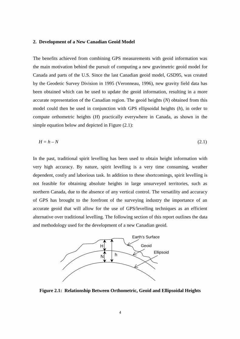
simple equation below and depicted in Figure (2.1):
H = h – N (2.1)
In the past, traditional spirit levelling has been used to obtain height information with
very high accuracy. By nature, spirit levelling is a very time consuming, weather
dependent, costly and laborious task. In addition to these shortcomings, spirit levelling is
not feasible for obtaining absolute heights in large unsurveyed territories, such as
northern Canada, due to the absence of any vertical control. The versatility and accuracy
of GPS has brought to the forefront of the surveying industry the importance of an
accurate geoid that will allow for the use of GPS/levelling techniques as an efficient
alternative over traditional levelling. The following section of this report outlines the data
and methodology used for the development of a new Canadian geoid.
Figure 2.1: Relationship Between Orthometric, Geoid and Ellipsoidal Heights
H
N h
Earth’s Surface
Geoid
Ellipsoid
5
2.1 Computational Methodology
The computation of the new Canadian geoid model (GARR98) was based on the classical
"remove-compute-restore" technique. The underlying procedure can be summarized as
follows:
1) Remove a gravity anomaly field (computed from a global spherical harmonic model
evaluated at the geoid) from Helmert gravity anomalies that are computed from local
surface gravity measurements and digital elevation data. In this way, "residual
Helmert anomalies" are obtained. Faye anomalies were actually used to approximate
the Helmert gravity anomalies.
2) Compute "residual co-geoid undulations" (N∆g) by a spherical Fourier representation
of Stokes’ convolution integral using the residual gravity anomalies.
3) Restore a geoid undulation field NGM (computed from a global spherical harmonic
model evaluated at the geoid) to the residual co-geoid undulations, and add also a
topographic indirect effect term NH (computed from digital elevation data) to form
the final geoid undulations.
The above three steps can be combined in a single formula as follows:
N = NGM + N∆g + NH (2.2)
The computation of the NGM term was made on a 5’ × 5’ grid, within the following
geographical boundaries: northern N72°, southern N41°, western W142°, and eastern
W53°. This is also the grid configuration in which the final GARR98 geoid heights are
given. The EGM96 geopotential model (complete to degree and order 360) was used for
these computations, according to the following formula (Heiskanen and Moritz, 1967):
∑∑= =
+=360
2 0
)(sin )]sin()cos(C[ n
n
mnmnmnmGM PmSmRN φλλ (2.3)
6
An initial comparison at the above grid between EGM96 and the OSU91A geopotential
model which was used in the development of the latest GSD95 Canadian geoid, showed
an RMS undulation difference of 97 cm. Further information and tests for the
performance of the EGM96 geopotential model over the Canadian region can be found in
IGeS (1997). Additional comparisons are presented in the following section of this report.
The medium and small wavelength contributions to the total geoid heights were
computed from the local gravity anomaly data, according to Stokes’ formula (Heiskanen
and Moritz, 1967)
∫ ∫∆=∆
Q Q
QQQPQQQPPg ddSgR
Nλ φ
λφφψλφπγ
λφ cos )( ),( 4
),( (2.4)
where S(ψ) is the Stokes function, and the local data ∆g are residual Faye anomalies, i.e.
GMFA gcgg ∆−+∆=∆ (2.5)
In the last equation, ∆gFA are the usual free-air anomalies, c is the terrain correction term,
and ∆gGM is the removed long wavelength contribution of the geopotential model
computed from the expression
( ) ( ) ( )ϕλλ sinP sincos1-nG nm0m
n
2n
max
∑∑==
+=∆n
nmnmGM mSmCg (2.6)
where nmC and nmS are normalized coefficients from a spherical harmonic series
expansion for the anomalous potential obtained from a global geopotential model data set
(EGM96 or OSU91A) and nmP are normalized Legendre functions. All the gravity data
were obtained from the Geodetic Survey Division (GSD) of Geomatics Canada in the
form of a 5’ × 5’ grid of mean Faye anomalies, within the same geographical boundaries
mentioned above. This is essentially a smaller part of the gravity grid used in the
7
development of the original GSD95 geoid model. The GSD95 gravity grid covered a
slightly larger region, which extended its eastern boundary to W46° and including half of
the Greenland area and most of the Labrador Sea. However, the GARR98 grid
incorporates some newly obtained surface gravity information across British Columbia,
which was not used in the GSD95 solution. The average spacing of the surface gravity
measurements used for the gridding was approximately 10 km on land, and 1 km over the
oceans in Canada. A detailed description of the Canadian gravity database and the
followed gridding procedures can be found in Veronneau (1995 and 1996). A discussion
for the treatment and computation of all the necessary gravity reductions (atmospheric,
free-air gradient, terrain reduction) applied to the original data is included in Veronneau
(1994) and Mainville et al. (1994).
The evaluation of Stokes’ integral (2.4) was performed by the 1D spherical FFT
algorithm (Haagmans et al., 1993), according to the expression
[ ] [ ]
∆∆∆= ∑=
−∆
max
1
cos ),( )( 4
),( 1φ
φφφλφψ
πγλφλφ
Q
QQQPQPPg gSR
N FFF (2.7)
where the operators F and F−1 denote the forward and inverse 1D discrete Fourier
transform, ∆φ = ∆λ = 5’ is the used grid spacing, and φ1, φmax are the southern and
northern grid boundaries, respectively. The gravity anomaly input grid (∆gcosφ) had 50%
zero padding applied on the east and west edges of the grid, but none on the north and
south sides. This is because equation (2.7) performs the FFT in the east/west direction,
and thus padding is only needed on those two edges to eliminate circular convolution
effects. On the other hand, the values of the Stokes spherical kernel S were analytically
computed at all points of the zero-padded grid, and its discrete spectrum values were
subsequently used in (2.7). Also, no tapering of ∆g was performed, since the long
wavelength part of the gravity anomaly signal had already been removed from the grid
values.
8
The shorter wavelength information for the GARR98 geoid model was obtained through
the computation of the indirect effect term NH, induced by using Helmert’s second
condensation method for the gravity data reduction on the geoid (Heiskanen and Moritz,
1967). In general, the formulation of the topographic indirect effect on the geoid,
according to Helmert’s second condensation method, is made in terms of a Taylor series
expansion from which only the first three terms are usually considered:
21 NNNN oH δδδ ++= (2.8)
Wichiencharoen (1982) and Sideris (1990) should be consulted for all the detailed
formulas. In our case, only the zero-order term
γρπδ
2
DEMo
HGN −= (2.9)
was used for the geoid computations, since it is the dominant one. The same
approximation was also adopted in the construction of the GSD95 geoid model. The
height data used to evaluate (2.9) were obtained from a 1km × 1km Digital Elevation
Model (DEM) which covered most of the Western Canadian region (N67°, N47°, W135°,
W110°). In contrast to the GSD95 geoid solution, which additionally used the global
ETOPO5-DEM and the Digital Terrain Elevation Data set (DTED-Level 1) to obtain a
total terrain coverage for Canada, no other height data sources were incorporated in the
GARR98 model. However, the DEM file that was used in the GARR98 geoid solution
provided us with a better overall terrain resolution for the Western mountainous parts of
Canada, since it was not restricted only in the Northern British Columbia and in the
Yukon Territory, as it happened with the corresponding 1km × 1km DEM used in the
GSD95 geoid solution (Veronneau, 1996).
9
2.2 GARR98
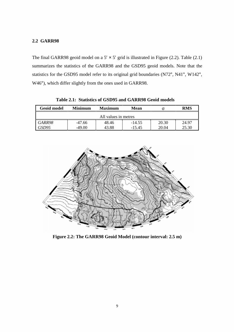
The final GARR98 geoid model on a 5′ × 5′ grid is illustrated in Figure (2.2). Table (2.1)
summarizes the statistics of the GARR98 and the GSD95 geoid models. Note that the
statistics for the GSD95 model refer to its original grid boundaries (N72°, N41°, W142°,
W46°), which differ slightly from the ones used in GARR98.
Table 2.1: Statistics of GSD95 and GARR98 Geoid models
Geoid model Minimum Maximum Mean σ RMS
All values in metresGARR98 -47.66 48.46 -14.55 20.30 24.97GSD95 -49.00 43.88 -15.45 20.04 25.30
Figure 2.2: The GARR98 Geoid Model (contour interval: 2.5 m)
10
3. Evaluation of Various Geoid Models
An important aspect during the development of a new gravimetric geoid for Canada was
its evaluation with already existing geoid models. Comparisons between GARR98 and
other models (GSD95, EGM96 and OSU91A) were conducted in order to assess the
accuracy of the models on both regional and national scales. In addition to inter-
comparisons between models, results for the absolute and relative agreement of these
geoid models with respect to GPS/levelling data are also provided. Finally, a sample of
the achievable orthometric height accuracies resulting by combining GPS heights derived
from a kinematic DGPS campaign and geoid heights, is provided to demonstrate the
feasibility of performing actual ‘GPS/levelling’.
3.1 Comparisons Between Geoid Models
In order to investigate the quality of the new gravimetric geoid, comparisons between
various geoid models were made by differencing their geoidal undulation values on the 5'
× 5' grid used to compute GARR98 (see Section 2.2). These differences are displayed
graphically on shaded contour plots in Figures (3.1) through (3.3), and their statistics are
given in Table (3.1).
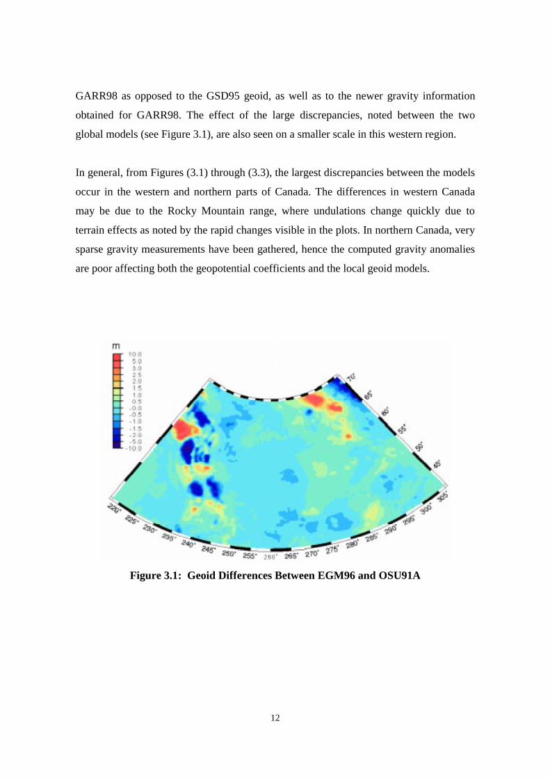
At first, a comparison between the EGM96 and OSU91A global geoid models is made,
and the result is illustrated in Figure (3.1). It reveals the strong effect of the additional
gravity data in the Western and in the Northeastern parts of Canada, which were
incorporated in the development of EGM96. This new gravity data results in up to 10
metre differences in geoidal undulations in Northwestern Canada and the area around
Greenland. Extreme differences are also seen in the Rocky Mountain region due to its
rugged terrain features, which suggests the importance of using dense gravity coverage in
order to recover the small-wavelength gravity field information. The highest level of
agreement between the two global models is found in Central Canada averaging up to 50
cm, which increases to up to 1.5 m in parts of Eastern Canada.
11
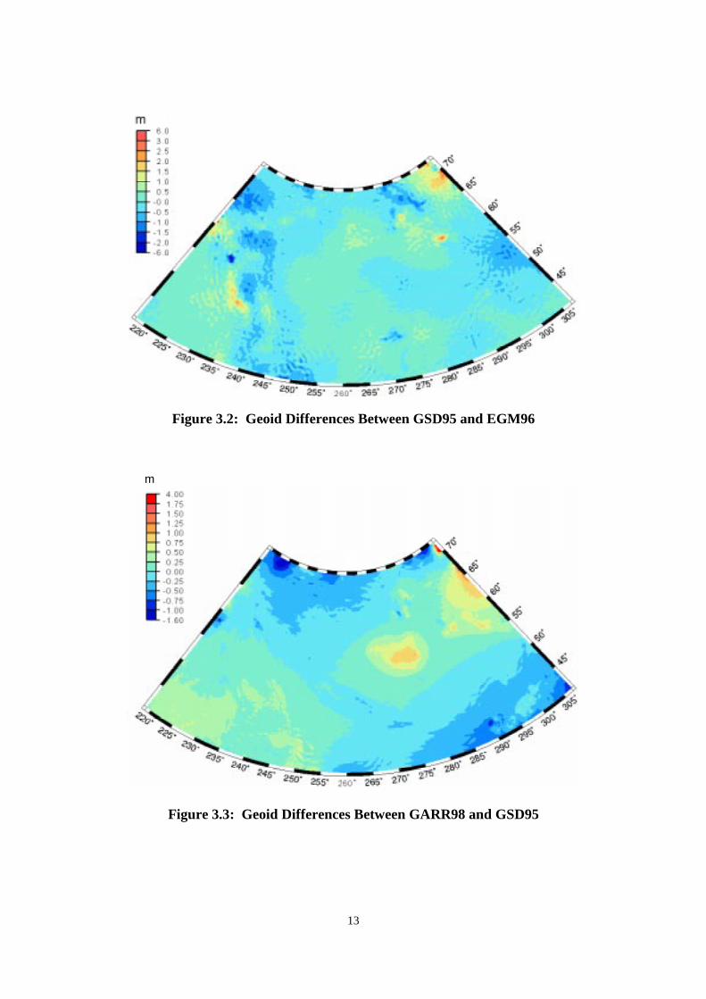
Figure (3.2) shows the differences between GSD95 and EGM96, which basically reveal
the medium and small wavelength structure of the Canadian gravity field, combined with
the discrepancies between EGM96 and OSU91A. It should be kept in mind that GSD95
uses the OSU91A model as a reference field. Again, the maximum differences between
the models are seen in the Western mountainous regions, as well as in the Northeastern
areas.
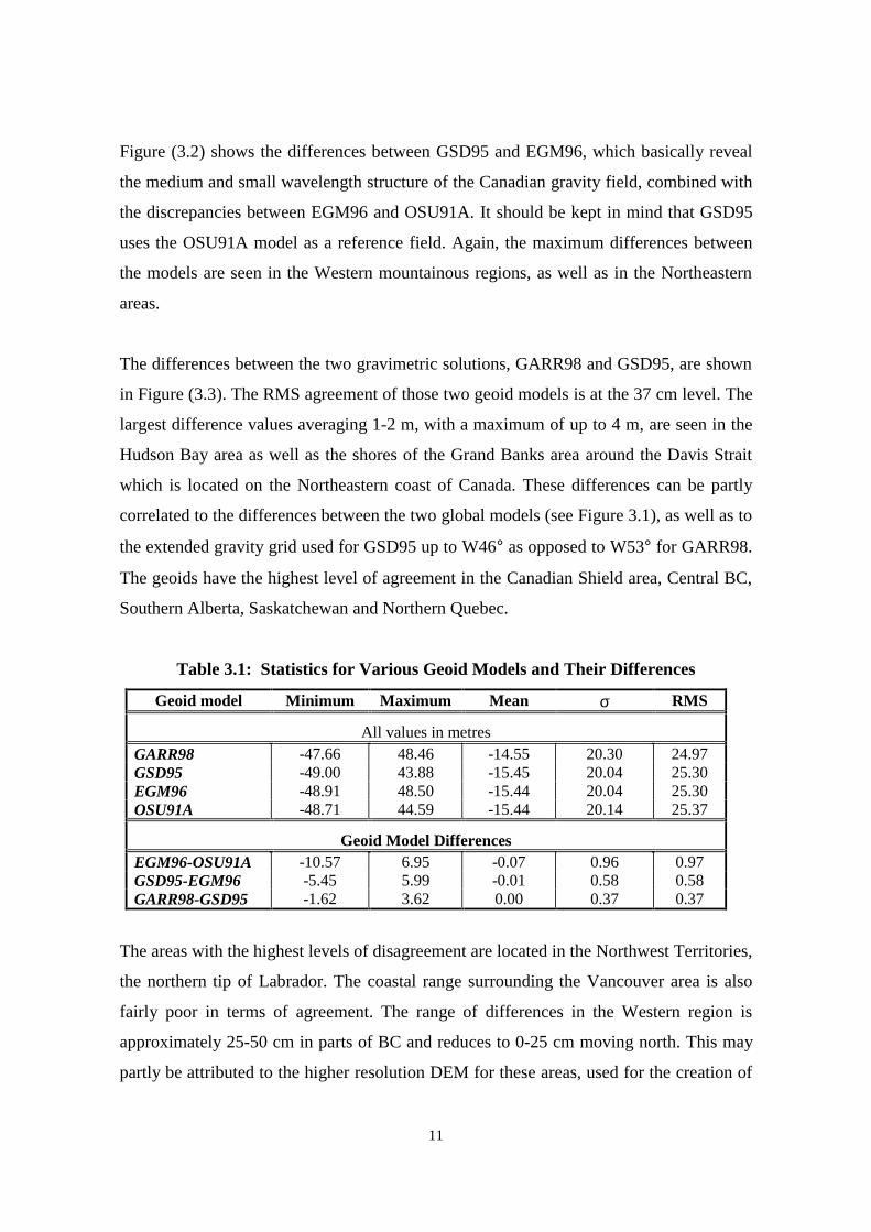
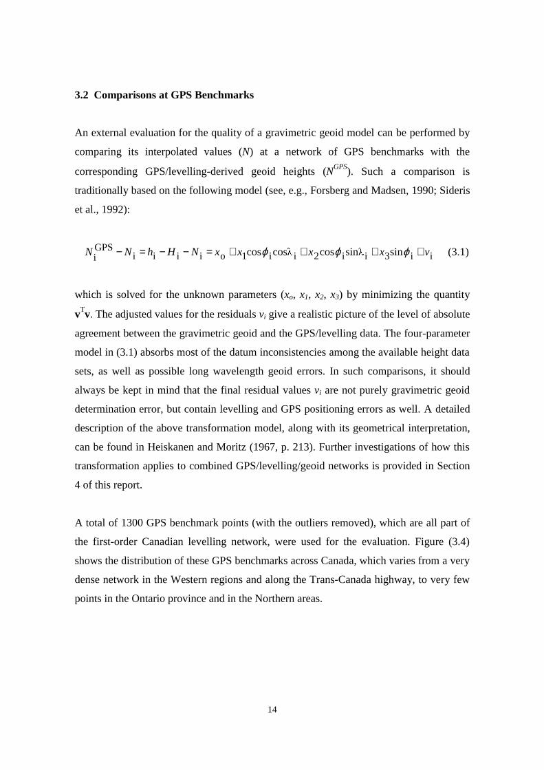
The differences between the two gravimetric solutions, GARR98 and GSD95, are shown
in Figure (3.3). The RMS agreement of those two geoid models is at the 37 cm level. The
largest difference values averaging 1-2 m, with a maximum of up to 4 m, are seen in the
Hudson Bay area as well as the shores of the Grand Banks area around the Davis Strait
which is located on the Northeastern coast of Canada. These differences can be partly
correlated to the differences between the two global models (see Figure 3.1), as well as to
the extended gravity grid used for GSD95 up to W46° as opposed to W53° for GARR98.
The geoids have the highest level of agreement in the Canadian Shield area, Central BC,
Southern Alberta, Saskatchewan and Northern Quebec.
Table 3.1: Statistics for Various Geoid Models and Their Differences
Geoid model Minimum Maximum Mean σ RMS
All values in metres GARR98 -47.66 48.46 -14.55 20.30 24.97 GSD95 -49.00 43.88 -15.45 20.04 25.30 EGM96 -48.91 48.50 -15.44 20.04 25.30 OSU91A -48.71 44.59 -15.44 20.14 25.37
Geoid Model Differences EGM96-OSU91A -10.57 6.95 -0.07 0.96 0.97 GSD95-EGM96 -5.45 5.99 -0.01 0.58 0.58 GARR98-GSD95 -1.62 3.62 0.00 0.37 0.37
The areas with the highest levels of disagreement are located in the Northwest Territories,
the northern tip of Labrador. The coastal range surrounding the Vancouver area is also
fairly poor in terms of agreement. The range of differences in the Western region is
approximately 25-50 cm in parts of BC and reduces to 0-25 cm moving north. This may
partly be attributed to the higher resolution DEM for these areas, used for the creation of
12
GARR98 as opposed to the GSD95 geoid, as well as to the newer gravity information
obtained for GARR98. The effect of the large discrepancies, noted between the two
global models (see Figure 3.1), are also seen on a smaller scale in this western region.
In general, from Figures (3.1) through (3.3), the largest discrepancies between the models
occur in the western and northern parts of Canada. The differences in western Canada
may be due to the Rocky Mountain range, where undulations change quickly due to
terrain effects as noted by the rapid changes visible in the plots. In northern Canada, very
sparse gravity measurements have been gathered, hence the computed gravity anomalies
are poor affecting both the geopotential coefficients and the local geoid models.
Figure 3.1: Geoid Differences Between EGM96 and OSU91A
13
Figure 3.2: Geoid Differences Between GSD95 and EGM96
Figure 3.3: Geoid Differences Between GARR98 and GSD95
m
14
3.2 Comparisons at GPS Benchmarks
An external evaluation for the quality of a gravimetric geoid model can be performed by
comparing its interpolated values (N) at a network of GPS benchmarks with the
corresponding GPS/levelling-derived geoid heights (NGPS). Such a comparison is
traditionally based on the following model (see, e.g., Forsberg and Madsen, 1990; Sideris
et al., 1992):
ii3ii2ii1oiiiiGPSi sinsincoscoscos vxxxxNHhNN ++++=−−=− ϕϕϕ (3.1)
which is solved for the unknown parameters (xo, x1, x2, x3) by minimizing the quantity
vTv. The adjusted values for the residuals vi give a realistic picture of the level of absolute
agreement between the gravimetric geoid and the GPS/levelling data. The four-parameter
model in (3.1) absorbs most of the datum inconsistencies among the available height data
sets, as well as possible long wavelength geoid errors. In such comparisons, it should
always be kept in mind that the final residual values vi are not purely gravimetric geoid
determination error, but contain levelling and GPS positioning errors as well. A detailed
description of the above transformation model, along with its geometrical interpretation,
can be found in Heiskanen and Moritz (1967, p. 213). Further investigations of how this
transformation applies to combined GPS/levelling/geoid networks is provided in Section
4 of this report.
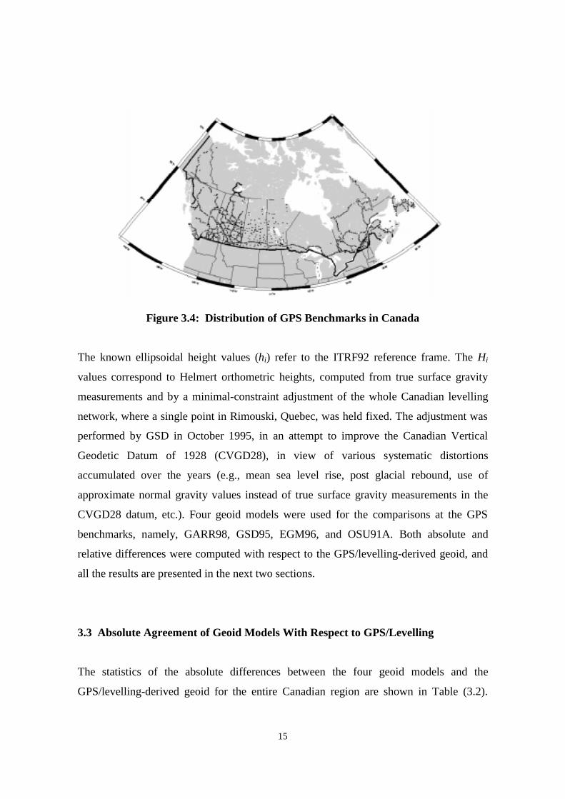
A total of 1300 GPS benchmark points (with the outliers removed), which are all part of
the first-order Canadian levelling network, were used for the evaluation. Figure (3.4)
shows the distribution of these GPS benchmarks across Canada, which varies from a very
dense network in the Western regions and along the Trans-Canada highway, to very few
points in the Ontario province and in the Northern areas.
15
Figure 3.4: Distribution of GPS Benchmarks in Canada
The known ellipsoidal height values (hi) refer to the ITRF92 reference frame. The Hi
values correspond to Helmert orthometric heights, computed from true surface gravity
measurements and by a minimal-constraint adjustment of the whole Canadian levelling
network, where a single point in Rimouski, Quebec, was held fixed. The adjustment was
performed by GSD in October 1995, in an attempt to improve the Canadian Vertical
Geodetic Datum of 1928 (CVGD28), in view of various systematic distortions
accumulated over the years (e.g., mean sea level rise, post glacial rebound, use of
approximate normal gravity values instead of true surface gravity measurements in the
CVGD28 datum, etc.). Four geoid models were used for the comparisons at the GPS
benchmarks, namely, GARR98, GSD95, EGM96, and OSU91A. Both absolute and
relative differences were computed with respect to the GPS/levelling-derived geoid, and
all the results are presented in the next two sections.
3.3 Absolute Agreement of Geoid Models With Respect to GPS/Levelling
The statistics of the absolute differences between the four geoid models and the
GPS/levelling-derived geoid for the entire Canadian region are shown in Table (3.2).
16
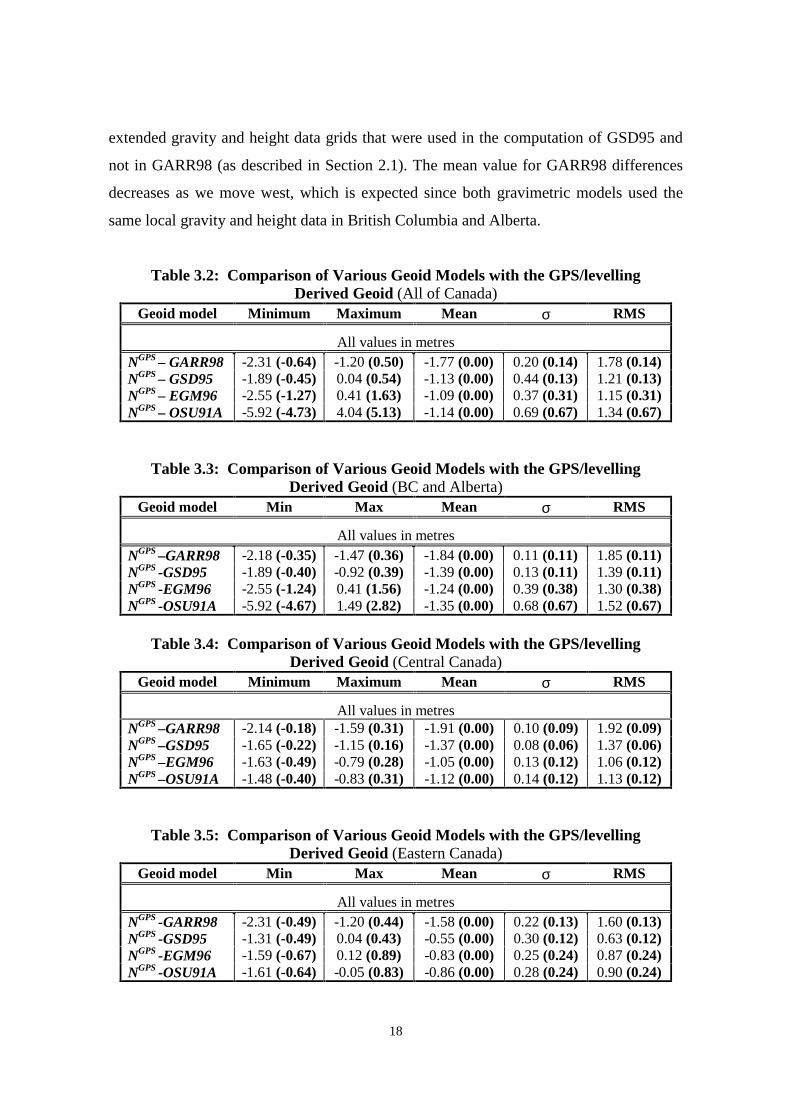
Three additional tables are given, in which the absolute agreement is studied for three
separate major regions in Canada. Table (3.3) refers to all GPS benchmarks in Alberta
and British Columbia (Western Canada); Table (3.4) uses all the GPS benchmarks lying
inside the meridian zone 95°W<λ<110°W (Central Canada); and finally Table (3.5) takes
into account only the GPS benchmarks east of 95°W (Eastern Canada). Note that the
values inside the parentheses, shown in all four tables, are the results after the least-
squares fitting of the 4-parameter transformation model has been applied to the original
differences. It should be noted that for the computation of all statistics presented in this
section, the GPS benchmarks showing large differences before the least-squares fitting
(i.e., >3σ level) were removed. The removal of such points with gross errors, in either the
GPS or levelling data, further improved the results obtained in previous computations
where no effort to remove the outliers was performed.
From the statistics shown in Table (3.2), it can be seen that the GARR98 gravimetrically
derived geoid, with the support of the EGM96 global model, drastically improves the
overall agreement with the GPS/levelling-derived geoid in Canada, from a σ of 44 cm to
a σ of 20 cm. After the fit, however, both GARR98 and GSD95 present approximately
the same overall external accuracy, which is at the 13-14 cm level. This would suggest
that even with the use of EGM96, the present gravity data accuracy and resolution still
needs to be improved in Canada, in order to bring the absolute geoid consistency with
GPS/levelling data down to the cm-level. It is also interesting to note the superiority of
the EGM96 global model, over OSU91A, for describing the long wavelength structure of
the Canadian gravity field. After the fit, EGM96 alone fits the Canadian GPS/levelling
geoid with an overall RMS accuracy of 31 cm, whereas OSU91A cannot perform better
than 67 cm on a national scale (more than 100% difference in accuracy). This is basically
due to the fact that OSU91A provides a very poor representation of gravity field features
over the British Columbia and Alberta regions, as seen from the corresponding values in
Table (3.3).
A regional analysis for the statistics of the differences reveals the interesting result of
having the same level of absolute agreement (after fit) for the gravimetric geoid solutions
17
in both Western and Eastern Canada. This is not surprising and it simply confirms that
the strong terrain gravity signal in the Western region has been properly modeled in both
GSD95 and GARR98 models. For the same area, the two global geoid models provide an
RMS agreement with the GPS/levelling data of 38 cm (EGM96) and 67 cm (OSU91A),
respectively, illustrating again the superiority of the EGM96 model.
In Central Canada, GSD95 seems to perform slightly better than GARR98, with the
former model giving an after fit RMS accuracy at the GPS benchmarks of 6 cm and the
latter 9 cm. A possible reason for this difference in accuracy between the two gravimetric
models may be the incorporation in the GSD95 solution of height data for this region, in
contrast to GARR98 which uses a DEM only for western Canada. In addition, no
improvement in EGM96 over OSU91A occurs in this area, which might have been
reflected in the corresponding local gravimetric solutions.
More interesting, however, is the fact that the use of GPS, in conjunction with a global
geoid model alone, seems to be sufficient for levelling applications in central Canada
requiring dm-level of accuracy. Both global models represent the gravity field in the
central flat areas quite well, with an agreement level of 12 cm for both EGM96 and
OSU91A. All four geoid models achieve their best performance in this area. For the
Eastern part of Canada, both gravimetric geoids show similar results, with GSD95 (12
cm) being marginally better than GARR98 (13 cm). Again, the fact that additional
gravity and height data in this region were used in the GSD95 solution (see Section 2) is
probably causing this difference. In the case where a global geoid model is only
employed for the Eastern region, the level of agreement worsens by more than 10 cm,
reaching 24 cm for both EGM96 and OSU91A.
In general, the GARR98 geoid model shows a large bias before the four-parameter
transformation (see also table 3.1). For example, in the Eastern region the difference in
the mean values between GARR98 and GSD95 is more than 1 m, whereas in the Western
region this difference drops to less that 50 cm. These high biased values are not due to the
differences between EGM96 and OSU91A, but rather they exist because of the more
18
extended gravity and height data grids that were used in the computation of GSD95 and
not in GARR98 (as described in Section 2.1). The mean value for GARR98 differences
decreases as we move west, which is expected since both gravimetric models used the
same local gravity and height data in British Columbia and Alberta.
Table 3.2: Comparison of Various Geoid Models with the GPS/levelling Derived Geoid (All of Canada)
Geoid model Minimum Maximum Mean σ RMS
All values in metres NGPS – GARR98 -2.31 (-0.64) -1.20 (0.50) -1.77 (0.00) 0.20 (0.14) 1.78 (0.14) NGPS – GSD95 -1.89 (-0.45) 0.04 (0.54) -1.13 (0.00) 0.44 (0.13) 1.21 (0.13) NGPS – EGM96 -2.55 (-1.27) 0.41 (1.63) -1.09 (0.00) 0.37 (0.31) 1.15 (0.31) NGPS – OSU91A -5.92 (-4.73) 4.04 (5.13) -1.14 (0.00) 0.69 (0.67) 1.34 (0.67)
Table 3.3: Comparison of Various Geoid Models with the GPS/levelling Derived Geoid (BC and Alberta)
Geoid model Min Max Mean σ RMS
All values in metres NGPS –GARR98 -2.18 (-0.35) -1.47 (0.36) -1.84 (0.00) 0.11 (0.11) 1.85 (0.11) NGPS -GSD95 -1.89 (-0.40) -0.92 (0.39) -1.39 (0.00) 0.13 (0.11) 1.39 (0.11) NGPS -EGM96 -2.55 (-1.24) 0.41 (1.56) -1.24 (0.00) 0.39 (0.38) 1.30 (0.38) NGPS -OSU91A -5.92 (-4.67) 1.49 (2.82) -1.35 (0.00) 0.68 (0.67) 1.52 (0.67)
Table 3.4: Comparison of Various Geoid Models with the GPS/levelling
Derived Geoid (Central Canada) Geoid model Minimum Maximum Mean σ RMS
All values in metres NGPS –GARR98 -2.14 (-0.18) -1.59 (0.31) -1.91 (0.00) 0.10 (0.09) 1.92 (0.09) NGPS –GSD95 -1.65 (-0.22) -1.15 (0.16) -1.37 (0.00) 0.08 (0.06) 1.37 (0.06) NGPS –EGM96 -1.63 (-0.49) -0.79 (0.28) -1.05 (0.00) 0.13 (0.12) 1.06 (0.12) NGPS –OSU91A -1.48 (-0.40) -0.83 (0.31) -1.12 (0.00) 0.14 (0.12) 1.13 (0.12)
Table 3.5: Comparison of Various Geoid Models with the GPS/levelling Derived Geoid (Eastern Canada)
Geoid model Min Max Mean σ RMS
All values in metres NGPS -GARR98 -2.31 (-0.49) -1.20 (0.44) -1.58 (0.00) 0.22 (0.13) 1.60 (0.13) NGPS -GSD95 -1.31 (-0.49) 0.04 (0.43) -0.55 (0.00) 0.30 (0.12) 0.63 (0.12) NGPS -EGM96 -1.59 (-0.67) 0.12 (0.89) -0.83 (0.00) 0.25 (0.24) 0.87 (0.24) NGPS -OSU91A -1.61 (-0.64) -0.05 (0.83) -0.86 (0.00) 0.28 (0.24) 0.90 (0.24)
19
An interesting observation can also be made by comparing the standard deviation values
shown in Tables (3.2) through (3.5), before and after the four-parameter model
adjustment. By doing such a comparison one sees that in Western and Central Canada the
accuracy improvement for all four geoid models, after the 4-parameter transformation, is
approximately constant and averages to about 1.75 cm. This amount is also very close to
the mean accuracy improvement for the two global models, occurring in Eastern Canada.
It is quite reasonable to assume that such a small amount should represent the difference
between the GPS datum and the datum used in the development of the global geoid
models, i.e., the reference frame realized by the satellite tracking station coordinates.
However, in Eastern Canada both GARR98 and GSD95 exhibit a large deviation from
this “1.75 cm accuracy improvement” trend, as it is seen from their corresponding values
in Table (3.5). This deviation could possibly be attributed to the fact that the parametric
model of eq.(3.1) not only eliminates the datum differences among the available data sets,
but also absorbs a part of gravimetric geoid random error, caused from the extended
amount of low-quality shipborne gravity data used in this area (see Section 4 for details).
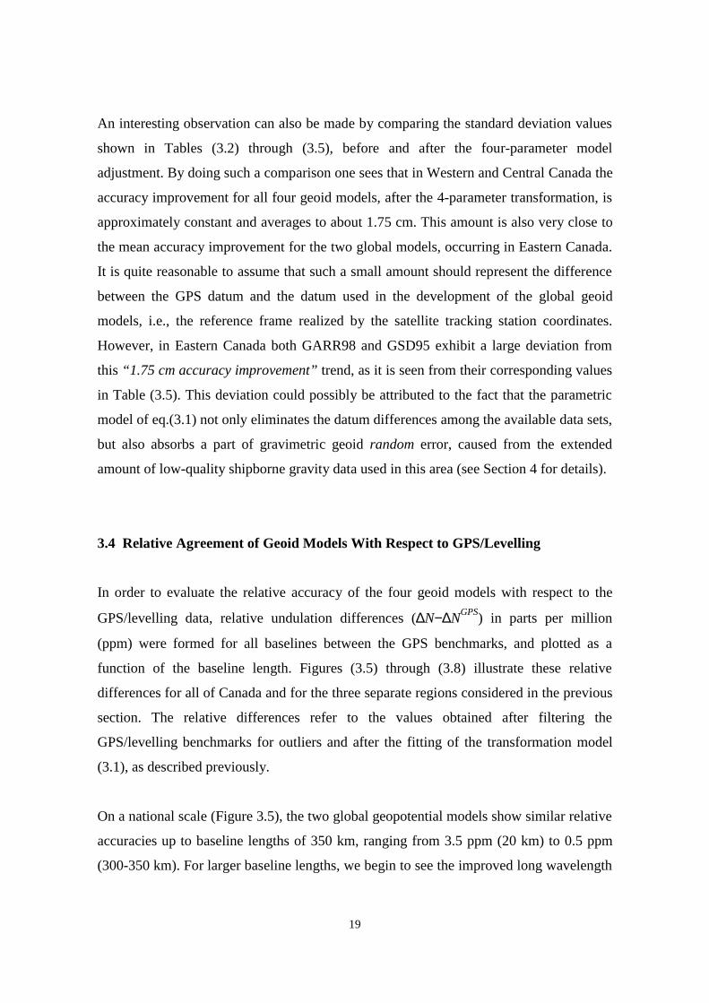
3.4 Relative Agreement of Geoid Models With Respect to GPS/Levelling
In order to evaluate the relative accuracy of the four geoid models with respect to the
GPS/levelling data, relative undulation differences (∆N−∆NGPS) in parts per million
(ppm) were formed for all baselines between the GPS benchmarks, and plotted as a
function of the baseline length. Figures (3.5) through (3.8) illustrate these relative
differences for all of Canada and for the three separate regions considered in the previous
section. The relative differences refer to the values obtained after filtering the
GPS/levelling benchmarks for outliers and after the fitting of the transformation model
(3.1), as described previously.
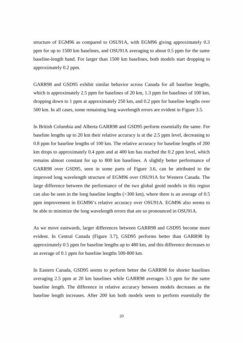
On a national scale (Figure 3.5), the two global geopotential models show similar relative
accuracies up to baseline lengths of 350 km, ranging from 3.5 ppm (20 km) to 0.5 ppm
(300-350 km). For larger baseline lengths, we begin to see the improved long wavelength
20
structure of EGM96 as compared to OSU91A, with EGM96 giving approximately 0.3
ppm for up to 1500 km baselines, and OSU91A averaging to about 0.5 ppm for the same
baseline-length band. For larger than 1500 km baselines, both models start dropping to
approximately 0.2 ppm.
GARR98 and GSD95 exhibit similar behavior across Canada for all baseline lengths,
which is approximately 2.5 ppm for baselines of 20 km, 1.3 ppm for baselines of 100 km,
dropping down to 1 ppm at approximately 250 km, and 0.2 ppm for baseline lengths over
500 km. In all cases, some remaining long wavelength errors are evident in Figure 3.5.
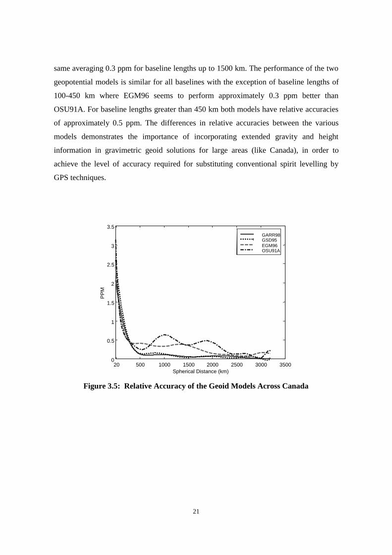
In British Columbia and Alberta GARR98 and GSD95 perform essentially the same. For
baseline lengths up to 20 km their relative accuracy is at the 2.5 ppm level, decreasing to
0.8 ppm for baseline lengths of 100 km. The relative accuracy for baseline lengths of 200
km drops to approximately 0.4 ppm and at 400 km has reached the 0.2 ppm level, which
remains almost constant for up to 800 km baselines. A slightly better performance of
GARR98 over GSD95, seen in some parts of Figure 3.6, can be attributed to the
improved long wavelength structure of EGM96 over OSU91A for Western Canada. The
large difference between the performance of the two global geoid models in this region
can also be seen in the long baseline lengths (>300 km), where there is an average of 0.5
ppm improvement in EGM96’s relative accuracy over OSU91A. EGM96 also seems to
be able to minimize the long wavelength errors that are so pronounced in OSU91A.
As we move eastwards, larger differences between GARR98 and GSD95 become more
evident. In Central Canada (Figure 3.7), GSD95 performs better than GARR98 by
approximately 0.5 ppm for baseline lengths up to 480 km, and this difference decreases to
an average of 0.1 ppm for baseline lengths 500-800 km.
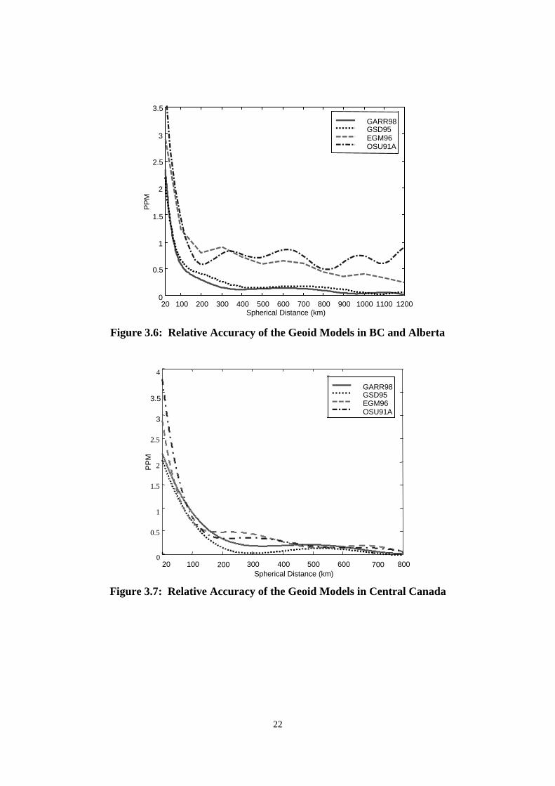
In Eastern Canada, GSD95 seems to perform better the GARR98 for shorter baselines
averaging 2.5 ppm at 20 km baselines while GARR98 averages 3.5 ppm for the same
baseline length. The difference in relative accuracy between models decreases as the
baseline length increases. After 200 km both models seem to perform essentially the
21
same averaging 0.3 ppm for baseline lengths up to 1500 km. The performance of the two
geopotential models is similar for all baselines with the exception of baseline lengths of
100-450 km where EGM96 seems to perform approximately 0.3 ppm better than
OSU91A. For baseline lengths greater than 450 km both models have relative accuracies
of approximately 0.5 ppm. The differences in relative accuracies between the various
models demonstrates the importance of incorporating extended gravity and height
information in gravimetric geoid solutions for large areas (like Canada), in order to
achieve the level of accuracy required for substituting conventional spirit levelling by
GPS techniques.
20 500 1000 1500 2000 2500 3000 35000
0.5
1
1.5
2
2.5
3
3.5
Spherical Distance (km)
PP
M
GARR98GSD95EGM96OSU91A
Figure 3.5: Relative Accuracy of the Geoid Models Across Canada
22
20 100 200 300 400 500 600 700 800 900 1000 1100 1200
0
0.5
1
1.5
2
2.5
3
3.5
Spherical Distance (km)
PP
M
GARR98GSD95EGM96OSU91A
Figure 3.6: Relative Accuracy of the Geoid Models in BC and Alberta
20 100 200 300 400 500 600 700 800
0
0.5
1
1.5
2
2.5
3
3.5
4
Spherical Distance (km)
PP
M
GARR98GSD95EGM96OSU91A
Figure 3.7: Relative Accuracy of the Geoid Models in Central Canada
23
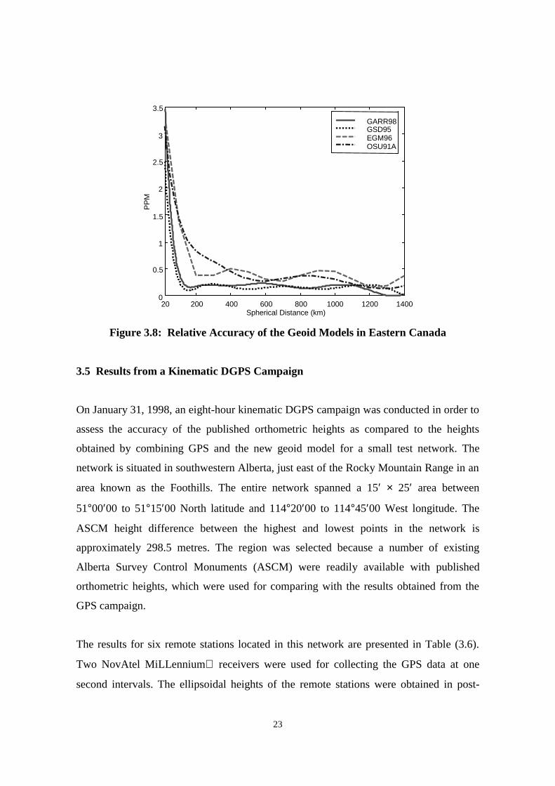
20 200 400 600 800 1000 1200 14000
0.5
1
1.5
2
2.5
3
3.5
Spherical Distance (km)
PP
M
GARR98GSD95EGM96OSU91A
Figure 3.8: Relative Accuracy of the Geoid Models in Eastern Canada
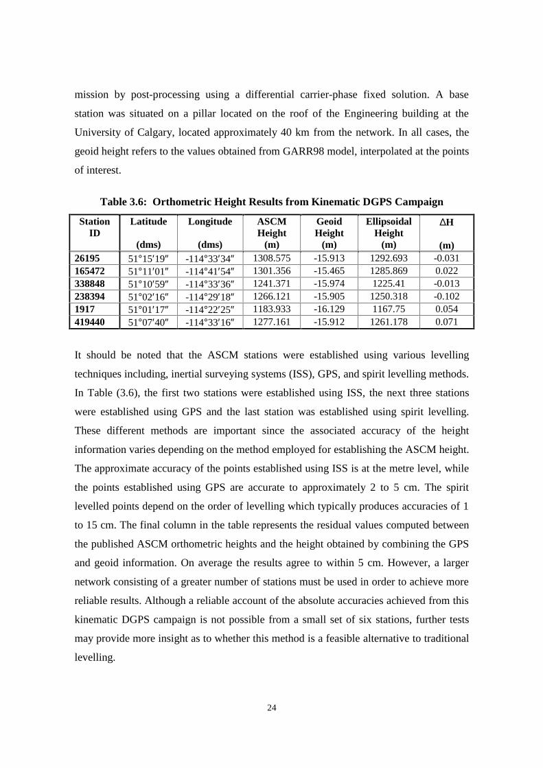
3.5 Results from a Kinematic DGPS Campaign
On January 31, 1998, an eight-hour kinematic DGPS campaign was conducted in order to
assess the accuracy of the published orthometric heights as compared to the heights
obtained by combining GPS and the new geoid model for a small test network. The
network is situated in southwestern Alberta, just east of the Rocky Mountain Range in an
area known as the Foothills. The entire network spanned a 15′ × 25′ area between
51°00′00 to 51°15′00 North latitude and 114°20′00 to 114°45′00 West longitude. The
ASCM height difference between the highest and lowest points in the network is
approximately 298.5 metres. The region was selected because a number of existing
Alberta Survey Control Monuments (ASCM) were readily available with published
orthometric heights, which were used for comparing with the results obtained from the
GPS campaign.
The results for six remote stations located in this network are presented in Table (3.6).
Two NovAtel MiLLennium receivers were used for collecting the GPS data at one
second intervals. The ellipsoidal heights of the remote stations were obtained in post-
24
mission by post-processing using a differential carrier-phase fixed solution. A base
station was situated on a pillar located on the roof of the Engineering building at the
University of Calgary, located approximately 40 km from the network. In all cases, the
geoid height refers to the values obtained from GARR98 model, interpolated at the points
of interest.
Table 3.6: Orthometric Height Results from Kinematic DGPS Campaign
StationID
Latitude
(dms)
Longitude
(dms)
ASCMHeight
(m)
GeoidHeight
(m)
EllipsoidalHeight
(m)
∆H
(m)26195 51°15′19″ -114°33′34″ 1308.575 -15.913 1292.693 -0.031165472 51°11′01″ -114°41′54″ 1301.356 -15.465 1285.869 0.022338848 51°10′59″ -114°33′36″ 1241.371 -15.974 1225.41 -0.013238394 51°02′16″ -114°29′18″ 1266.121 -15.905 1250.318 -0.1021917 51°01′17″ -114°22′25″ 1183.933 -16.129 1167.75 0.054419440 51°07′40″ -114°33′16″ 1277.161 -15.912 1261.178 0.071
It should be noted that the ASCM stations were established using various levelling
techniques including, inertial surveying systems (ISS), GPS, and spirit levelling methods.
In Table (3.6), the first two stations were established using ISS, the next three stations
were established using GPS and the last station was established using spirit levelling.
These different methods are important since the associated accuracy of the height
information varies depending on the method employed for establishing the ASCM height.
The approximate accuracy of the points established using ISS is at the metre level, while
the points established using GPS are accurate to approximately 2 to 5 cm. The spirit
levelled points depend on the order of levelling which typically produces accuracies of 1
to 15 cm. The final column in the table represents the residual values computed between
the published ASCM orthometric heights and the height obtained by combining the GPS
and geoid information. On average the results agree to within 5 cm. However, a larger
network consisting of a greater number of stations must be used in order to achieve more
reliable results. Although a reliable account of the absolute accuracies achieved from this
kinematic DGPS campaign is not possible from a small set of six stations, further tests
may provide more insight as to whether this method is a feasible alternative to traditional
levelling.
25
4. Adjustment of Combined GPS/Levelling/Geoid Networks
The combined use of GPS, levelling, and geoid information has been a key procedure for
various geodetic applications. Although these three types of height information are
considerably different in terms of physical meaning, reference surface
definition/realization, observational methods, accuracy, etc., they should fulfill the simple
geometrical relationship (see also equation 2.1):
0=−− NHh (4.1)
where h, H, and N are as described in Section 2.1. In practice equation (4.1) is never
satisfied due to (i) random noise in the values of h, H, N, (ii) datum inconsistencies and
other possible systematic distortions in the three height data sets (e.g. long-wavelength
systematic errors in N, distortions in the vertical datum due to an overconstrained
adjustment of the levelling network, deviation between gravimetric geoid and reference
surface of the levelling datum, etc.), (iii) various geodynamic effects (post glacial
rebound, land subsidence, plate deformation near subduction zones, mean sea level rise,
monument instabilities), and (iv) theoretical approximations in the computation of either
H or N (e.g. improper or omitted terrain/density modeling in the geoid solution, improper
evaluation of Helmert’s formula for orthometric heights using normal gravity values
instead of actual surface gravity observations, negligence of the Sea Surface Topography
(SST) at the tide gauges, error-free assumption for the tide gauge observations, etc.). The
statistical behavior and modelling of the misclosures of equation (4.1), computed in a
network of levelled GPS benchmarks, have been the subject of many studies which are
often considerably different in terms of their research objectives. The following is a non-
exhaustive list for some of these objectives. The references provided are just
representative and not the only important ones.
(1) Testing the performance of global spherical harmonic models for the Earth’s
gravitational field (IGeS, 1997), or testing the performance of local/regional
26
gravimetric geoid models and their associated computational techniques
(Mainville et al., 1992; Sideris et al., 1992).
(2) Development of intermediate corrector surfaces for optimal height
transformation between geoid surface and levelling datum surface (Mainville et
al., 1997; Smith and Milbert, 1996).
(3) Development of corrector surfaces for low-wavelength gravimetric geoid errors
(De Bruijne et al., 1997), and general gravimetric geoid refinement strategies
(Jiang and Duquenne, 1996).
(4) Evaluation of the achievable accuracy for ‘levelling by GPS’ surveys (Forsberg
and Madsen, 1990).
(5) Monitoring, testing, and/or improving (strengthening) of already existed vertical
datums (Hein, 1986; Kearsley et al., 1993).
The above list can be further extended if we substitute the GPS height h in equation (4.1)
with altimetric observations, and the orthometric height H with the SST. A study for such
marine applications is included in De Bruijne et al. (1997). In view of the many different
uses for such multi-data 1D networks, the purpose of this section is to present some
general adjustment and modelling schemes that can be employed for an optimal analysis
of the misclosures of equation (4.1). In particular, we are mainly interested in
applications of the type (1), (2), or (3) from the previous list.
4.1 Overview of Various Adjustment Schemes
A brief review of various adjustment and modelling schemes, that have been already
applied for the applications mentioned in the previous section, will be given here. Some
general aspects for adjustment problems with combined height data sets can be found in
Pelzer (1986).
27
4.1.1 Geoid Evaluation
Most of the geoid evaluation studies, based on comparisons with GPS/levelling data,
make use of the following basic model:
iiiii vNHh T +=−− xa (4.2)
where x is a vector of n unknown parameters, ia is an n×1 vector of known coefficients,
and iv denotes a residual random noise term. The parametric part xaTi is supposed to
describe all possible datum inconsistencies and other systematic effects in the data sets.
In practice, for these studies, the usual four-parameter model is often used, i.e.
iiiiioi xxxx ϕλϕλϕ sinsincoscoscos 321T +++=xa (4.3)
and rarely its five-parameter extension (see, e.g., Duquenne et al., 1995)
iiiiiioi xxxxx ϕϕλϕλϕ 24321
T sinsinsincoscoscos ++++=xa (4.4)
has also been employed. Both equations (4.3) and (4.4) correspond to the following
datum transformation model for the geoid undulation N, which is described extensively in
Heiskanen and Moritz (1967, sec.5-9):
iiiiiiiN ϕϕλϕλϕ 2ooo sinfasinZsincosYcoscosXa ∆+∆+∆+∆+∆=∆ (4.5)
where ooo Z,Y,X ∆∆∆ are the shift parameters between two ‘parallel’ datums and
af, ∆∆ are the changes in flattening and semi-major axis of the corresponding ellipsoids.
In our case, the two different datums will correspond to (i) the GPS datum and (ii) the
datum used for the development of the global spherical harmonic model that supports the
gravimetric geoid, and for the computation of the gravity anomaly data ∆g. The model of
28
equation (4.2) is applied to all network points and a least-squares adjustment is performed
to estimate the residuals iv , which are traditionally taken as the final external indication
of the geoid accuracy. The main problem under this approach is that the iv terms will
contain a combined amount of GPS, levelling, and geoid random error, that needs to be
separated into its individual components for a more reliable geoid assessment.
Furthermore, an optimal adjustment in a statistical sense would require the proper
weighting of the residuals, which is hardly applied in practice. Finally, the use of such
oversimplified parametric models, like (4.3) or (4.4), combined with improper weighting
of the residuals iv , create important problems in terms of the ‘separability’ of the various
random and systematic effects between the two unknown components xaTi and iv .
4.1.2 Corrector Surface for GPS/levelling
The development of such corrector surfaces aims basically at providing GPS users with
an optimal transformation model between ellipsoidal heights h and orthometric heights H
with respect to a given levelling datum. For a general discussion regarding theoretical and
practical aspects of this problem, see Featherstone (1998). Two such developments have
been reported in North America, particularly in the U.S. by the National Geodetic Survey
(NGS; Smith and Milbert, 1996) and in Canada by the Geodetic Survey Division (GSD;
Mainville et al., 1997). Both studies followed a similar methodology, using initially the
basic model of equation (4.2) with its parametric part given by equation (4.3). The
obtained adjusted values for the residuals iv were then spatially modelled in a grid form
using an interpolation procedure. In the GSD study, a minimum-curvature interpolation
algorithm was used, whereas NGS fitted an isotropic Gaussian covariance function to the
statistics of the irregularly distributed values iv and then used simple collocation
formulas for the gridding. From the combination of the gridded values for the residuals
and the adjusted values for the parameters x , a corrector surface was finally computed.
Some comments regarding the drawbacks of these modelling approaches will be given
later on in this chapter.
29
4.1.3 Gravimetric Geoid Refinement
In De Bruijne et al. (1997), a 28-parameter surface model was estimated to correct the
gravimetrically-derived geoid in the North Sea area for its long-wavelength errors.
TOPEX altimetric data (h) and gravimetric geoid heights (N) were only used in the
general observation equation (2), since the SST was neglected in this study. The
parametric model xaTi was comprised from a simple bi-linear part with 4 parameters (1
bias, 2 tilts, 1 torsion), and a more complicated part of trigonometric polynomials with 24
coefficients. For the optimal estimation of this correction model only the external
altimetric data were properly weighted, according to their precomputed standard
deviations. Extensive statistical testing was also applied to validate the final adjustment
results. For the refinement of land gravimetric geoid models using GPS/levelling data,
Jiang and Duquenne (1996) proposed the division of the entire test area into smaller
adjacent networks, in order to better model the higher frequency geoid distortions due to
the insufficient local gravity data coverage and the errors in the used DTMs.
4.1.4 Vertical Datum Testing/Refinement
For such applications, the analyzed network usually contains a combination of some, or
all, of the following data: (i) relative ∆H from conventional levelling, (ii) relative ∆h
from local GPS surveys, (iii) N or ∆N from a geoid model, (iv) absolute H and SST
values at tide gauge stations, and (v) absolute h from SLR or global GPS campaigns. The
above general data configuration was proposed by Kearsley et al. (1993). In their
extensive study for investigating the quality of sample subsets of the Australian Height
Datum (AHD), they used the following general mathematical model for known
observations and unknown parameters:
ijhijij vhhh ∆+−=∆ (4.6a)
ijHijij vHHH ∆+−=∆ (4.6b)
30
ijNijij vNNN ∆+−=∆ (4.6c)
0=−− jjj NHh (4.6d)
All available observations ),,( ijijij NHh ∆∆∆ , along with their a-priori accuracy
estimates, were simultaneously adjusted, using equation (4.6d) as a geometrical
constraint for the unknown parameters at each station point j. For the unknown
parameters, additional a-priori information can also be incorporated in the adjustment
algorithm (Bayesian estimation), in the form of independent point measurements with
their associated variances and possible co-variances (e.g., measurement of H at tide
gauge sites). The above methodology suggests a powerful adjustment tool that can be
used for vertical datum refinement/redefinition, where both geometrical (GPS, SLR) and
physical (levelling, geoid, mean sea level) quantities are optimally combined in a unified
IDVKLRQ��VHH�DOVR�9DQLþHN��������
Among the critical issues existing in this approach (as well as in the previously
overviewed applications) is the estimation of the a-priori covariance matrices for the
different data sets. Since these types of weighting measures are only used to describe the
behavior of the random errors in the measurements, some augmentation of the
observation equations (4.6) by additional auxiliary parametric models, describing
possible systematic/datum offsets in the available data sets, should also be considered.
4.2 General Modeling Considerations
In general, equation (4.1) does not hold exactly due to not only the presence of zero-mean
random errors in the height data, but also due to a number of other direct or indirect
systematic effects. Since there are not usually available a-priori corrections for many of
these effects, they should be individually modelled and estimated during an adjustment
process. In this way, the following three general equations can be written for each point
Pi in a combined GPS/Levelling/Geoid (GLG) network:
31
hi
hi
aii vfhh ++= , H
iH
iaii vfHH ++= , N
iN
iaii vfNN ++= (4.7)
where hi, Hi, and Ni denote the available ‘observed’ values for the GPS, orthometric and
geoid heights, respectively. The superscript α denotes true values with respect to a
unified geodetic datum, such that the following equation holds:
0=−− ai
ai
ai NHh (4.8)
The fi terms correspond to all the necessary reductions that need to be applied to the
original data in order to eliminate the datum inconsistencies and other systematic errors.
Finally, the vi terms describe zero-mean random noise errors, for which a second-order
stochastic model is available:
{ } hhh Cvv =TE , { } HHH Cvv =TE , { } NNN Cvv =TE (4.9)
For the orthometric heights, the covariance (CV) matrix CH is known from the
adjustment of the levelling network. In the same way, Ch can be computed from the
adjustment of the GPS surveys performed at the levelled benchmarks. In the gravimetric
geoid case, the covariance matrix CN is computed by simple error propagation from the
original noisy data used in the geoid solution (geopotential coefficients, gravity
anomalies, terrain heights); for detailed formulas, see Li and Sideris (1994). For a more
realistic stochastic error model, full knowledge of the CV matrices should not be
assumed. This is especially true for the geoid heights where the often vaguely known
noise level of the input data (GM coefficients, gravity, DTM) and the always necessary
stationary noise assumption when fast spectral techniques are employed for the
computations, may cause CN to deviate considerably from reality. Hence, we will adopt
the following stochastic model for the random noise effects in the three height data sets:
{ } hhhh Qvv E 2T σ= , { } HHHH Qvv E 2T σ= , { } NNNN Qvv E 2T σ= (4.10)
32
where the co-factor matrices Qh, QH, and QN are assumed known from the sources
previously indicated, and the three variance components are treated as unknown
parameters controlling the validity of the a-priori random error models. One could also
extend the above stochastic model a little bit more, by decomposing the covariance
matrix CN into two different CV matrices with associated unknown variance components,
which would correspond to the two main geoid random error sources (noisy geopotential
coefficients, noisy gravity anomaly data). In this report, the set of the observation
equations (4.7) and their associated stochastic model in equation (4.10) represent the
basic framework upon which all the derivations in the following sections will be based.
4.3 A General Adjustment Model
Let us assume that, at each point Pi of a test network with m points, we have a triplet of
height observations (hi, Hi, Ni), or equivalently one ‘synthetic’ observation li = hi−Hi−Ni.
By combining equations (4.7) and (4.8), we get the following observation equation for
each network point:
l h H N f f f v v vi i i i ih
iH
iN
ih
iH
iN= − − = − − + − −( ) ( ) (4.11)
or, in a more compact form
Ni
Hi
hiii vvvfl −−+= (4.12)
If the main objective for using such a test network is to evaluate the gravimetric geoid
accuracy, then we are naturally interested in the estimation of the viN terms. Since there
is a stochastic model (equation 4.10) that has been associated with these terms, the values
of viN are supposed to reflect all the geoid random error sources that were taken into
account for the computation of the matrix QN. Furthermore, the ability to estimate the
33
unknown parameter σ N2 according to some variance component estimation algorithm
(see, e.g., Rao, 1971; Rao, 1997), provides probably the most powerful statistical tool for
a reliable estimate of the actual geoid noise, and a useful means of testing all the
assumptions that were incorporated in the construction of the preliminary geoid error
model QN. There is still, however, an amount of geoid error which is not included in the
viN terms, and for which no a-priori information is available in general. We can very
briefly mention: aliasing effects, improper (or omitted) terrain and density modelling,
various biases in the coefficients of the geopotential model, etc. Such geoid errors, which
do not follow a zero-mean random behavior, will be absorbed in the fi correction term
along with many other systematic effects in the GPS and levelling data. In the absence of
any prior statistical and/or deterministic information for these error sources, filtering
them out and estimating their magnitude individually is impossible.
If, on the other hand, this test network is to be used for the determination of an optimal
corrector surface for future GPS/levelling applications, then the values if have to be
estimated and spatially modeled in the best possible way. The random noise terms
vih , vi
H , viN should be left out of the modeling for such a correction surface. This can be
easily realized by looking at the form of the basic observation equation in a future
orthometric height network, which will utilize GPS/geoid information, as well as the
computed corrector surface from our original test network, i.e.
vHcNh +=−− (4.13)
where the term c represents the reduction effect of the computed correction model. A
system of equations, created by taking the differences of equation (4.13) between the
GPS survey points, has now to be adjusted for the optimal estimation of the orthometric
height differences ∆H with respect to the local levelling datum. Correcting, prior to this
adjustment, the ‘GPS/geoid observations’ for their random noise effects (which is the
case if the terms vih and vi
N from equation (4.12) are included in the modeling of the
corrector surface term c) makes no sense statistically. Furthermore, if the residual values
34
viH from equation (4.12) are included in the modeling of the corrector surface, then the
available original observations in equation (4.13) will be ‘corrected’ for an error source
which does not even exist in them!
Let us now return to our initial observation model of equation (4.12). The correction term
)P( ii ff = represents a 2D spatial field of values, and it can be further decomposed in
the general form:
f si i i T= +a x (4.14)
where ai is an (n×1) vector of known coefficients, and x is an (n×1) vector of unknown
deterministic parameters. The term si denotes some ‘residual correction’, the nature of
which (deterministic or stochastic) is left unspecified for now. The final observation
equation for each point in the test network will have, therefore, the form:
Ni
Hi
hiiii vvvsl −−++= xaT (4.15)
and by using matrix notation in order to combine all the network points, we get
BvsAxl ++= (4.16)
where
[ ]T1 mi lll LL=l , [ ]s = s s si m1 L LT
(4.17a)
[ ]v v v v= h H NT T T T
(4.17b)
[ ] NHhvvv mi , , : # , #
T###1 LL=v (4.17c)
[ ]A a a a T= 1 L Li m (4.17d)
35
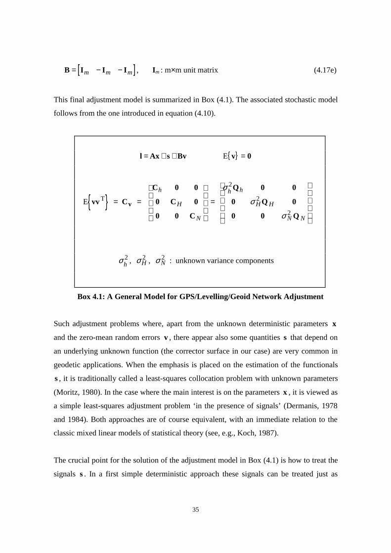
[ ]B I I I= − −m m m , Im : m×m unit matrix (4.17e)
This final adjustment model is summarized in Box (4.1). The associated stochastic model
follows from the one introduced in equation (4.10).
BvsAxl ++= { }E v 0=
{ }E Tvv C
C 0 0
0 C 0
0 0 C
Q 0 0
0 Q 0
0 0 Q
v= =
=
h
H
N
h h
H H
N N
σ
σ
σ
2
2
2
σh2 , σH
2 , σ N2 : unknown variance components
Box 4.1: A General Model for GPS/Levelling/Geoid Network Adjustment
Such adjustment problems where, apart from the unknown deterministic parameters x
and the zero-mean random errors v , there appear also some quantities s that depend on
an underlying unknown function (the corrector surface in our case) are very common in
geodetic applications. When the emphasis is placed on the estimation of the functionals
s , it is traditionally called a least-squares collocation problem with unknown parameters
(Moritz, 1980). In the case where the main interest is on the parameters x , it is viewed as
a simple least-squares adjustment problem ‘in the presence of signals’ (Dermanis, 1978
and 1984). Both approaches are of course equivalent, with an immediate relation to the
classic mixed linear models of statistical theory (see, e.g., Koch, 1987).
The crucial point for the solution of the adjustment model in Box (4.1) is how to treat the
signals s . In a first simple deterministic approach these signals can be treated just as
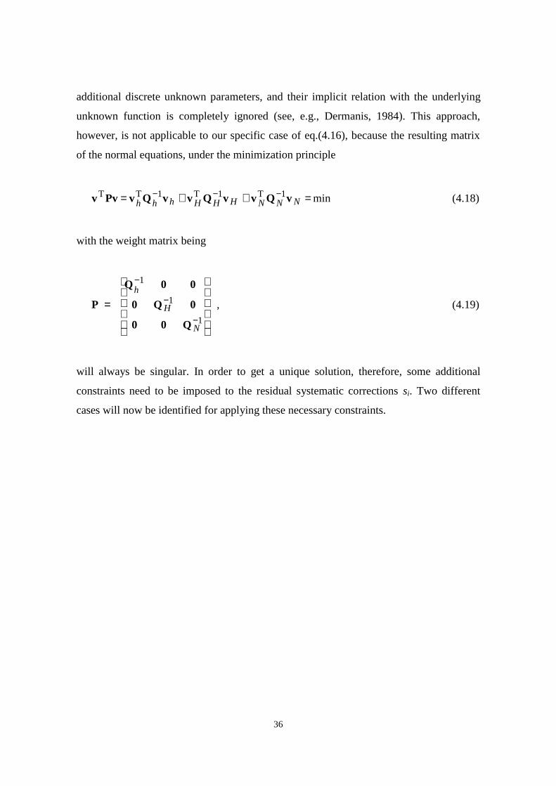
36
additional discrete unknown parameters, and their implicit relation with the underlying
unknown function is completely ignored (see, e.g., Dermanis, 1984). This approach,
however, is not applicable to our specific case of eq.(4.16), because the resulting matrix
of the normal equations, under the minimization principle
min 1T1T1TT =++= −−−NNNHHHhhh vQvvQvvQvPvv (4.18)
with the weight matrix being
P
Q 0 0
0 Q 0
0 0 Q
=
−
−
−
h
H
N
1
1
1
, (4.19)
will always be singular. In order to get a unique solution, therefore, some additional
constraints need to be imposed to the residual systematic corrections si. Two different
cases will now be identified for applying these necessary constraints.
37
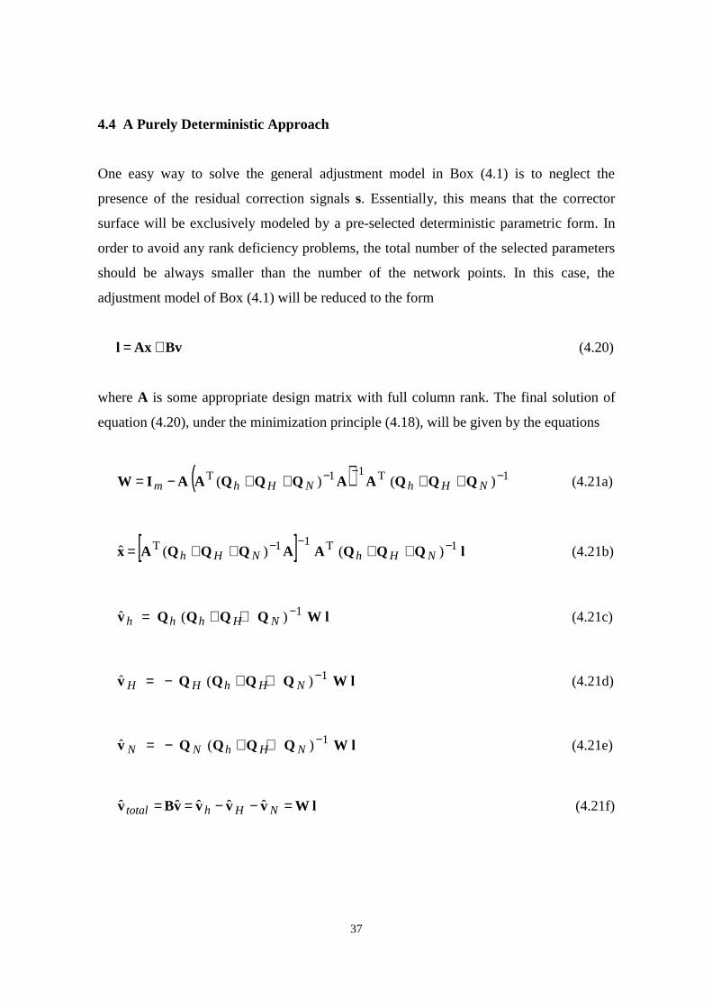
4.4 A Purely Deterministic Approach
One easy way to solve the general adjustment model in Box (4.1) is to neglect the
presence of the residual correction signals s. Essentially, this means that the corrector
surface will be exclusively modeled by a pre-selected deterministic parametric form. In
order to avoid any rank deficiency problems, the total number of the selected parameters
should be always smaller than the number of the network points. In this case, the
adjustment model of Box (4.1) will be reduced to the form
BvAxl += (4.20)
where A is some appropriate design matrix with full column rank. The final solution of
equation (4.20), under the minimization principle (4.18), will be given by the equations
( ) 1T11T )( )( −−− ++++−= NHhNHhm QQQAAQQQAAIW (4.21a)
[ ] lQQQAAQQQAx )( )( ˆ 1T11T −−− ++++= NHhNHh (4.21b)
$v Q Q Q Q W lh h h H N ( ) = + + −1 (4.21c)
$v Q Q Q Q W lH H h H N ( ) = − + + −1 (4.21d)
$v Q Q Q Q W lN N h H N ( ) = − + + −1 (4.21e)
lWvvvvBv ˆˆˆ ˆ ˆ =−−== NHhtotal (4.21f)
38
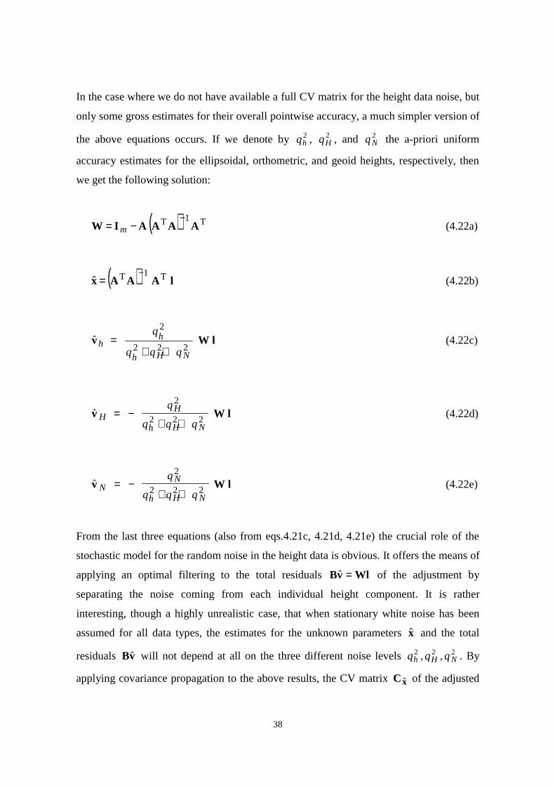
In the case where we do not have available a full CV matrix for the height data noise, but
only some gross estimates for their overall pointwise accuracy, a much simpler version of
the above equations occurs. If we denote by qh2 , qH
2 , and qN2 the a-priori uniform
accuracy estimates for the ellipsoidal, orthometric, and geoid heights, respectively, then
we get the following solution:
( ) T1T AAAAIW−
−= m (4.22a)
( ) lAAAx ˆ T1T −= (4.22b)
$v W lhh
h H N
q
q q q =
+ +
2
2 2 2 (4.22c)
$v W lHH
h H N
q
q q q = −
+ +
2
2 2 2 (4.22d)
$v W lNN
h H N
q
q q q = −
+ +
2
2 2 2 (4.22e)
From the last three equations (also from eqs.4.21c, 4.21d, 4.21e) the crucial role of the
stochastic model for the random noise in the height data is obvious. It offers the means of
applying an optimal filtering to the total residuals Bv Wl$ = of the adjustment by
separating the noise coming from each individual height component. It is rather
interesting, though a highly unrealistic case, that when stationary white noise has been
assumed for all data types, the estimates for the unknown parameters x and the total
residuals Bv$ will not depend at all on the three different noise levels qh2 , qH
2 , qN2 . By
applying covariance propagation to the above results, the CV matrix xC ˆ of the adjusted
39
model parameters can be also determined, which should be always used to evaluate the
quality of the parametric corrector surface for future GPS/levelling applications. Another
useful matrix is also the cross-CV matrix between the adjusted model parameters and the
adjusted residuals for the various height data sets, from which important information can
be extracted regarding the correlation of the corrector surface with the available data.
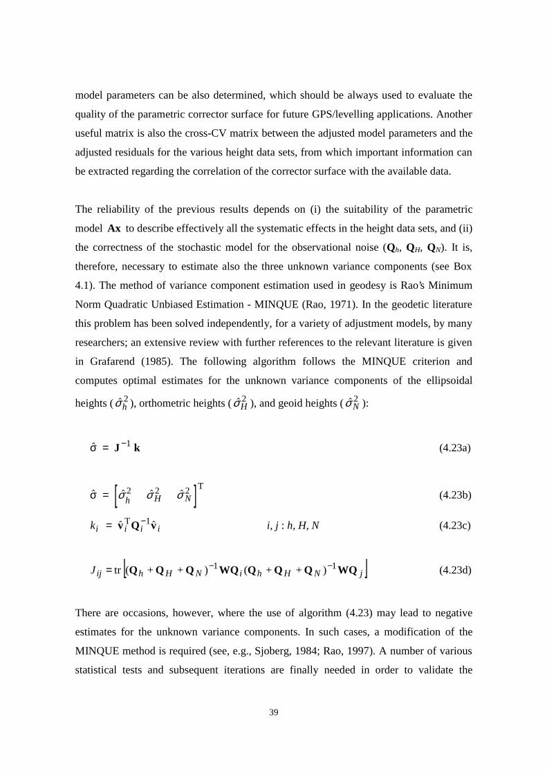
The reliability of the previous results depends on (i) the suitability of the parametric
model Ax to describe effectively all the systematic effects in the height data sets, and (ii)
the correctness of the stochastic model for the observational noise (Qh, QH, QN). It is,
therefore, necessary to estimate also the three unknown variance components (see Box
4.1). The method of variance component estimation used in geodesy is Rao’s Minimum
Norm Quadratic Unbiased Estimation - MINQUE (Rao, 1971). In the geodetic literature
this problem has been solved independently, for a variety of adjustment models, by many
researchers; an extensive review with further references to the relevant literature is given
in Grafarend (1985). The following algorithm follows the MINQUE criterion and
computes optimal estimates for the unknown variance components of the ellipsoidal
heights ( $σh2 ), orthometric heights ( $σH
2 ), and geoid heights ( $σ N2 ):
$σ = −J k1 (4.23a)
[ ]$ $ $ $σ T
= σ σ σh H N2 2 2 (4.23b)
ki i i i T= −$ $v Q v1 i, j : h, H, N (4.23c)
[ ]jNHhiNHhijJ WQQQQWQQQQ 11 )++()++( tr −−= (4.23d)
There are occasions, however, where the use of algorithm (4.23) may lead to negative
estimates for the unknown variance components. In such cases, a modification of the
MINQUE method is required (see, e.g., Sjoberg, 1984; Rao, 1997). A number of various
statistical tests and subsequent iterations are finally needed in order to validate the
40
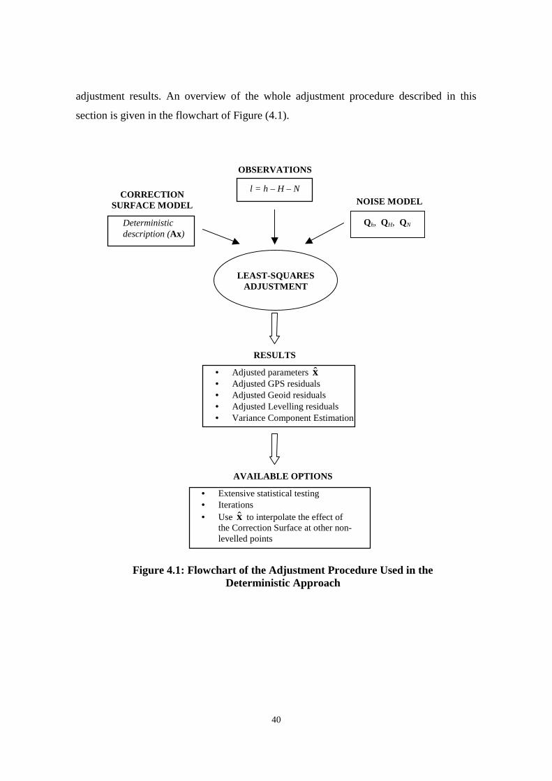
adjustment results. An overview of the whole adjustment procedure described in this
section is given in the flowchart of Figure (4.1).
Figure 4.1: Flowchart of the Adjustment Procedure Used in theDeterministic Approach
OBSERVATIONS
l = h – H – N
NOISE MODEL
Qh, QH, QN
CORRECTIONSURFACE MODEL
Deterministicdescription (Ax)
LEAST-SQUARESADJUSTMENT
RESULTS
• Adjusted parameters x• Adjusted GPS residuals• Adjusted Geoid residuals• Adjusted Levelling residuals• Variance Component Estimation
AVAILABLE OPTIONS
• Extensive statistical testing• Iterations• Use x to interpolate the effect of
the Correction Surface at other non-levelled points
41
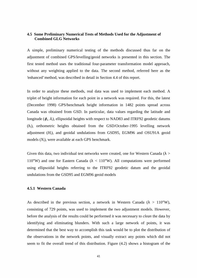
4.5 Some Preliminary Numerical Tests of Methods Used for the Adjustment ofCombined GLG Networks
A simple, preliminary numerical testing of the methods discussed thus far on the
adjustment of combined GPS/levelling/geoid networks is presented in this section. The
first tested method uses the traditional four-parameter transformation model approach,
without any weighting applied to the data. The second method, referred here as the
’enhanced’ method, was described in detail in Section 4.4 of this report.
In order to analyze these methods, real data was used to implement each method. A
triplet of height information for each point in a network was required. For this, the latest
(December 1998) GPS/benchmark height information in 1482 points spread across
Canada was obtained from GSD. In particular, data values regarding the latitude and
longitude (ϕi, λi), ellipsoidal heights with respect to NAD83 and ITRF92 geodetic datums
(hi), orthometric heights obtained from the GSD/October-1995 levelling network
adjustment (Hi), and geoidal undulations from GSD95, EGM96 and OSU91A geoid
models (Ni), were available at each GPS benchmark.
Given this data, two individual test networks were created, one for Western Canada (λ >
110°W) and one for Eastern Canada (λ < 110°W). All computations were performed
using ellipsoidal heights referring to the ITRF92 geodetic datum and the geoidal
undulations from the GSD95 and EGM96 geoid models
4.5.1 Western Canada
As described in the previous section, a network in Western Canada (λ > 110°W),
consisting of 729 points, was used to implement the two adjustment models. However,
before the analysis of the results could be performed it was necessary to clean the data by
identifying and eliminating blunders. With such a large network of points, it was
determined that the best way to accomplish this task would be to plot the distribution of
the observations in the network points, and visually extract any points which did not
seem to fit the overall trend of this distribution. Figure (4.2) shows a histogram of the
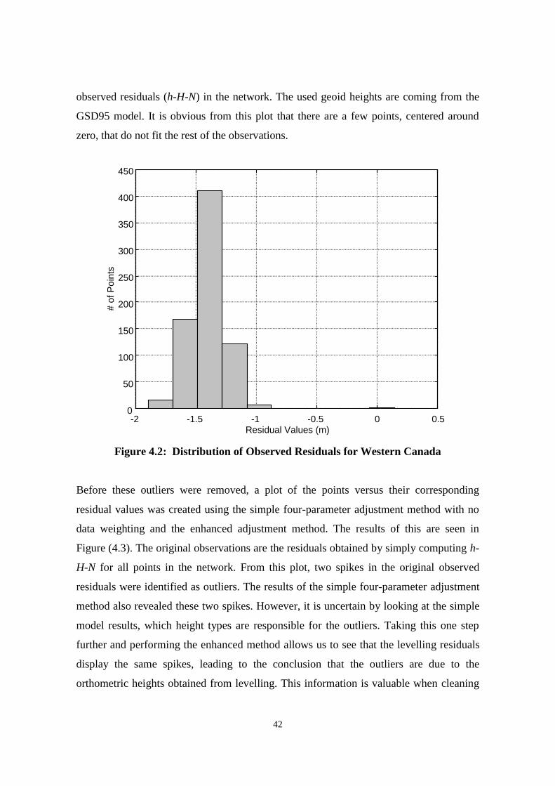
42
observed residuals (h-H-N) in the network. The used geoid heights are coming from the
GSD95 model. It is obvious from this plot that there are a few points, centered around
zero, that do not fit the rest of the observations.
-2 -1.5 -1 -0.5 0 0.50
50
100
150
200
250
300
350
400
450
Residual Values (m)
# of
Poi
nts
Figure 4.2: Distribution of Observed Residuals for Western Canada
Before these outliers were removed, a plot of the points versus their corresponding
residual values was created using the simple four-parameter adjustment method with no
data weighting and the enhanced adjustment method. The results of this are seen in
Figure (4.3). The original observations are the residuals obtained by simply computing h-
H-N for all points in the network. From this plot, two spikes in the original observed
residuals were identified as outliers. The results of the simple four-parameter adjustment
method also revealed these two spikes. However, it is uncertain by looking at the simple
model results, which height types are responsible for the outliers. Taking this one step
further and performing the enhanced method allows us to see that the levelling residuals
display the same spikes, leading to the conclusion that the outliers are due to the
orthometric heights obtained from levelling. This information is valuable when cleaning
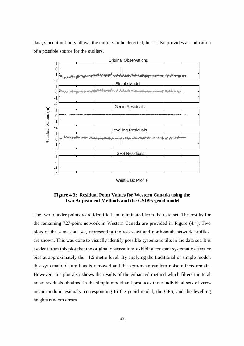
43
data, since it not only allows the outliers to be detected, but it also provides an indication
of a possible source for the outliers.
-2-101
Original Observations
-2-101
Simple Model
-2-101
Geoid Residuals
Res
idua
l Val
ues
(m)
-2-101
Levelling Residuals
-2-101
GPS Residuals
West-East Profile
Figure 4.3: Residual Point Values for Western Canada using theTwo Adjustment Methods and the GSD95 geoid model
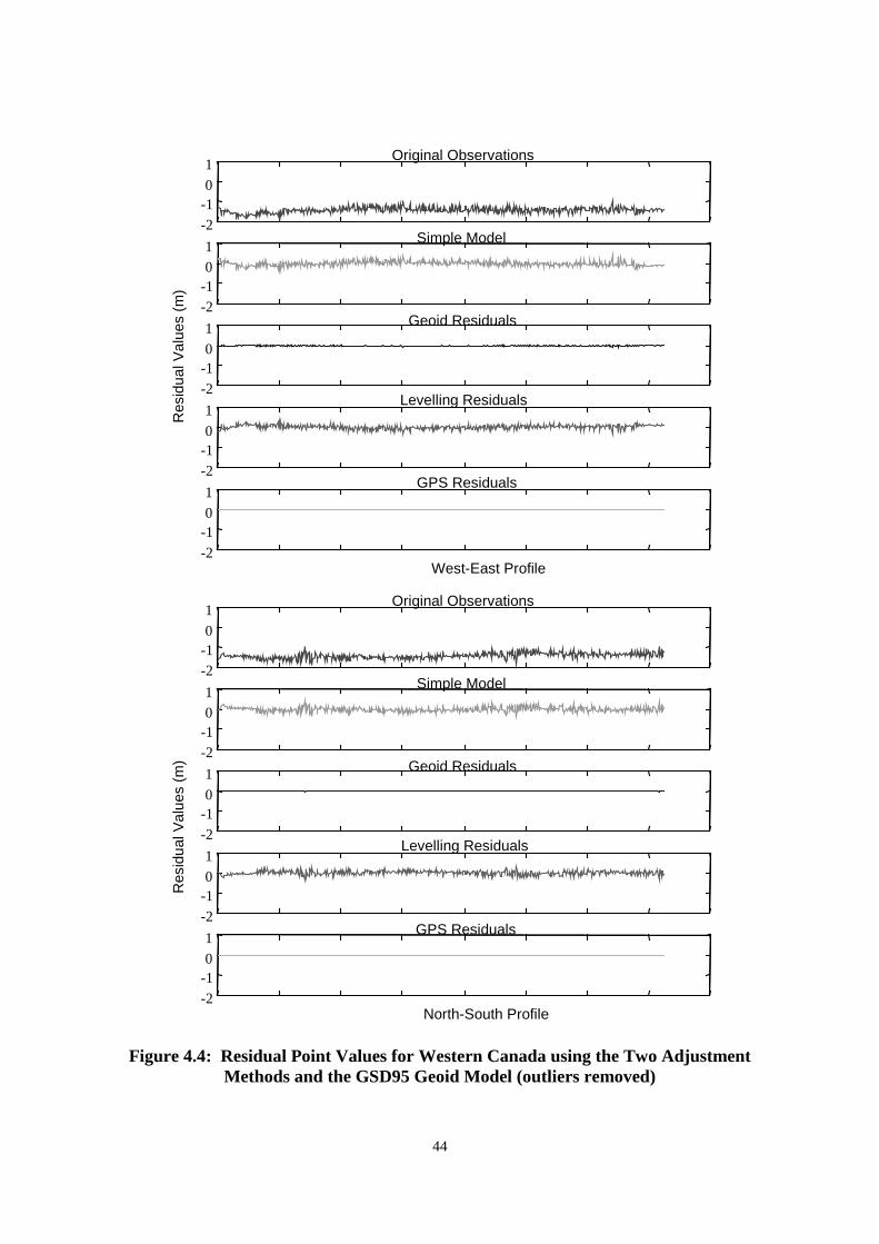
The two blunder points were identified and eliminated from the data set. The results for
the remaining 727-point network in Western Canada are provided in Figure (4.4). Two
plots of the same data set, representing the west-east and north-south network profiles,
are shown. This was done to visually identify possible systematic tilts in the data set. It is
evident from this plot that the original observations exhibit a constant systematic effect or
bias at approximately the –1.5 metre level. By applying the traditional or simple model,
this systematic datum bias is removed and the zero-mean random noise effects remain.
However, this plot also shows the results of the enhanced method which filters the total
noise residuals obtained in the simple model and produces three individual sets of zero-
mean random residuals, corresponding to the geoid model, the GPS, and the levelling
heights random errors.
44
-2-10
1Original Observations
-2-101
Simple Model
-2
-10
1 Geoid Residuals
Res
idua
l Val
ues
(m)
-2
-10
1Levelling Residuals
-2
-10
1GPS Residuals
West-East Profile
-2-10
1Original Observations
-2-101
Simple Model
-2
-10
1 Geoid Residuals
Res
idua
l Val
ues
(m)
-2
-10
1Levelling Residuals
-2
-10
1GPS Residuals
North-South Profile
Figure 4.4: Residual Point Values for Western Canada using the Two AdjustmentMethods and the GSD95 Geoid Model (outliers removed)
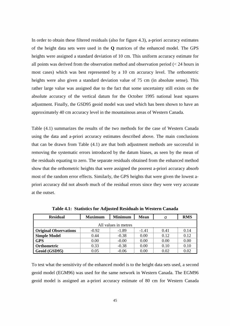
45
In order to obtain these filtered residuals (also for figure 4.3), a-priori accuracy estimates
of the height data sets were used in the Q matrices of the enhanced model. The GPS
heights were assigned a standard deviation of 10 cm. This uniform accuracy estimate for
all points was derived from the observation method and observation period (< 24 hours in
most cases) which was best represented by a 10 cm accuracy level. The orthometric
heights were also given a standard deviation value of 75 cm (in absolute sense). This
rather large value was assigned due to the fact that some uncertainty still exists on the
absolute accuracy of the vertical datum for the October 1995 national least squares
adjustment. Finally, the GSD95 geoid model was used which has been shown to have an
approximately 40 cm accuracy level in the mountainous areas of Western Canada.
Table (4.1) summarizes the results of the two methods for the case of Western Canada
using the data and a-priori accuracy estimates described above. The main conclusions
that can be drawn from Table (4.1) are that both adjustment methods are successful in
removing the systematic errors introduced by the datum biases, as seen by the mean of
the residuals equating to zero. The separate residuals obtained from the enhanced method
show that the orthometric heights that were assigned the poorest a-priori accuracy absorb
most of the random error effects. Similarly, the GPS heights that were given the lowest a-
priori accuracy did not absorb much of the residual errors since they were very accurate
at the outset.
Table 4.1: Statistics for Adjusted Residuals in Western Canada
Residual Maximum Minimum Mean σ RMS
All values in metresOriginal Observations -0.92 -1.89 -1.41 0.41 0.14Simple Model 0.44 -0.38 0.00 0.12 0.12GPS 0.00 -0.00 0.00 0.00 0.00Orthometric 0.33 -0.38 0.00 0.10 0.10Geoid (GSD95) 0.05 -0.06 0.00 0.02 0.02
To test what the sensitivity of the enhanced model is to the height data sets used, a second
geoid model (EGM96) was used for the same network in Western Canada. The EGM96
geoid model is assigned an a-priori accuracy estimate of 80 cm for Western Canada
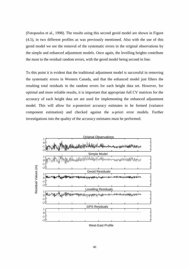
46
(Fotopoulos et al., 1998). The results using this second geoid model are shown in Figure
(4.5), in two different profiles as was previously mentioned. Also with the use of this
geoid model we see the removal of the systematic errors in the original observations by
the simple and enhanced adjustment models. Once again, the levelling heights contribute
the most to the residual random errors, with the geoid model being second in line.
To this point it is evident that the traditional adjustment model is successful in removing
the systematic errors in Western Canada, and that the enhanced model just filters the
resulting total residuals in the random errors for each height data set. However, for
optimal and more reliable results, it is important that appropriate full CV matrices for the
accuracy of each height data set are used for implementing the enhanced adjustment
model. This will allow for a-posteriori accuracy estimates to be formed (variance
component estimation) and checked against the a-priori error models. Further
investigations into the quality of the accuracy estimates must be performed.
-2-101
Original Observations
-2-101
Simple Model
-2-101
Geoid Residuals
Res
idua
l Val
ues
(m)
-2-101
Levelling Residuals
-2-101
GPS Residuals
West-East Profile
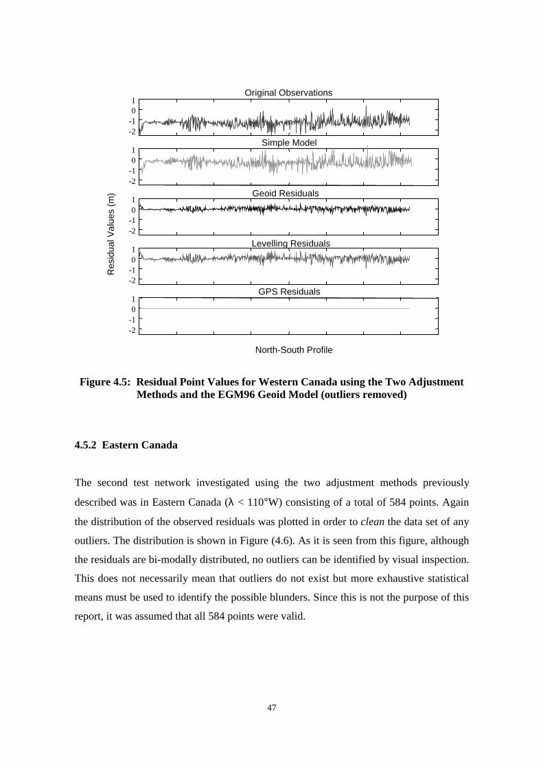
47
-2-101
Original Observations
-2-101
Simple Model
-2-101
Geoid Residuals
Res
idua
l Val
ues
(m)
-2-101
Levelling Residuals
-2-101
GPS Residuals
North-South Profile
Figure 4.5: Residual Point Values for Western Canada using the Two AdjustmentMethods and the EGM96 Geoid Model (outliers removed)
4.5.2 Eastern Canada
The second test network investigated using the two adjustment methods previously
described was in Eastern Canada (λ < 110°W) consisting of a total of 584 points. Again
the distribution of the observed residuals was plotted in order to clean the data set of any
outliers. The distribution is shown in Figure (4.6). As it is seen from this figure, although
the residuals are bi-modally distributed, no outliers can be identified by visual inspection.
This does not necessarily mean that outliers do not exist but more exhaustive statistical
means must be used to identify the possible blunders. Since this is not the purpose of this
report, it was assumed that all 584 points were valid.
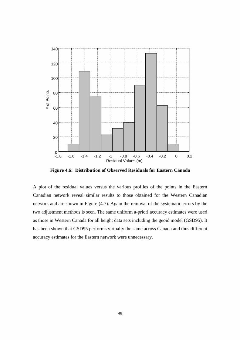
48
-1.8 -1.6 -1.4 -1.2 -1 -0.8 -0.6 -0.4 -0.2 0 0.20
20
40
60
80
100
120
140
Residual Values (m)
# of
Poi
nts
Figure 4.6: Distribution of Observed Residuals for Eastern Canada
A plot of the residual values versus the various profiles of the points in the Eastern
Canadian network reveal similar results to those obtained for the Western Canadian
network and are shown in Figure (4.7). Again the removal of the systematic errors by the
two adjustment methods is seen. The same uniform a-priori accuracy estimates were used
as those in Western Canada for all height data sets including the geoid model (GSD95). It
has been shown that GSD95 performs virtually the same across Canada and thus different
accuracy estimates for the Eastern network were unnecessary.
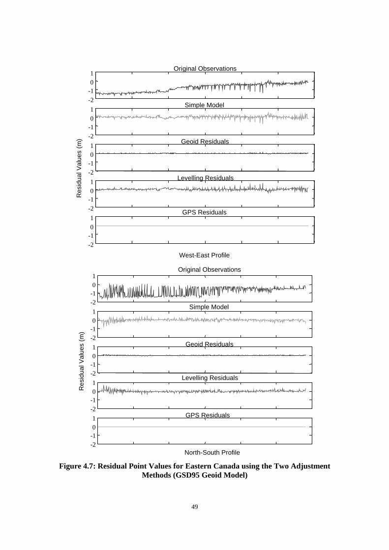
49
-2
-101
Original Observations
-2-101
Simple Model
-2-101
Geoid Residuals
Res
idua
l Val
ues
(m)
-2-10
1Levelling Residuals
-2
-10
1GPS Residuals
West-East Profile
-2-101
Original Observations
-2-101
Simple Model
-2-101 Geoid Residuals
Res
idua
l Val
ues
(m)
-2-101
Levelling Residuals
-2-101 GPS Residuals
North-South Profile
Figure 4.7: Residual Point Values for Eastern Canada using the Two AdjustmentMethods (GSD95 Geoid Model)
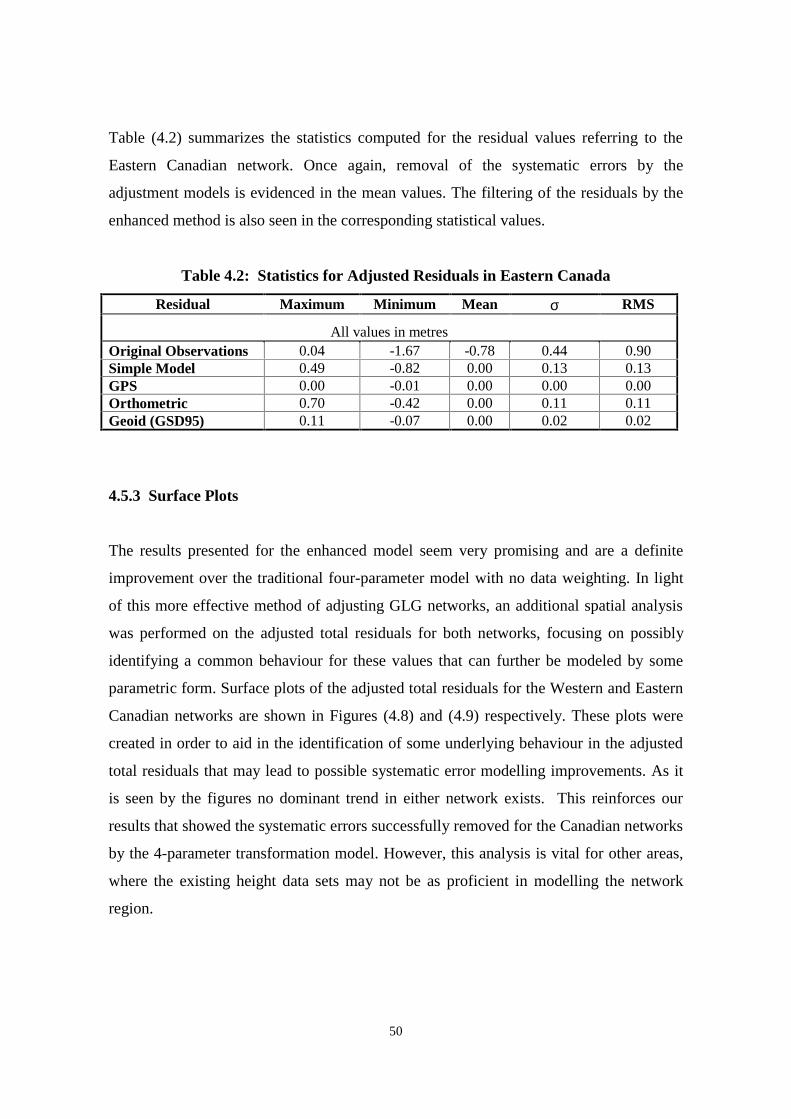
50
Table (4.2) summarizes the statistics computed for the residual values referring to the
Eastern Canadian network. Once again, removal of the systematic errors by the
adjustment models is evidenced in the mean values. The filtering of the residuals by the
enhanced method is also seen in the corresponding statistical values.
Table 4.2: Statistics for Adjusted Residuals in Eastern Canada
Residual Maximum Minimum Mean σ RMS
All values in metresOriginal Observations 0.04 -1.67 -0.78 0.44 0.90Simple Model 0.49 -0.82 0.00 0.13 0.13GPS 0.00 -0.01 0.00 0.00 0.00Orthometric 0.70 -0.42 0.00 0.11 0.11Geoid (GSD95) 0.11 -0.07 0.00 0.02 0.02
4.5.3 Surface Plots
The results presented for the enhanced model seem very promising and are a definite
improvement over the traditional four-parameter model with no data weighting. In light
of this more effective method of adjusting GLG networks, an additional spatial analysis
was performed on the adjusted total residuals for both networks, focusing on possibly
identifying a common behaviour for these values that can further be modeled by some
parametric form. Surface plots of the adjusted total residuals for the Western and Eastern
Canadian networks are shown in Figures (4.8) and (4.9) respectively. These plots were
created in order to aid in the identification of some underlying behaviour in the adjusted
total residuals that may lead to possible systematic error modelling improvements. As it
is seen by the figures no dominant trend in either network exists. This reinforces our
results that showed the systematic errors successfully removed for the Canadian networks
by the 4-parameter transformation model. However, this analysis is vital for other areas,
where the existing height data sets may not be as proficient in modelling the network
region.
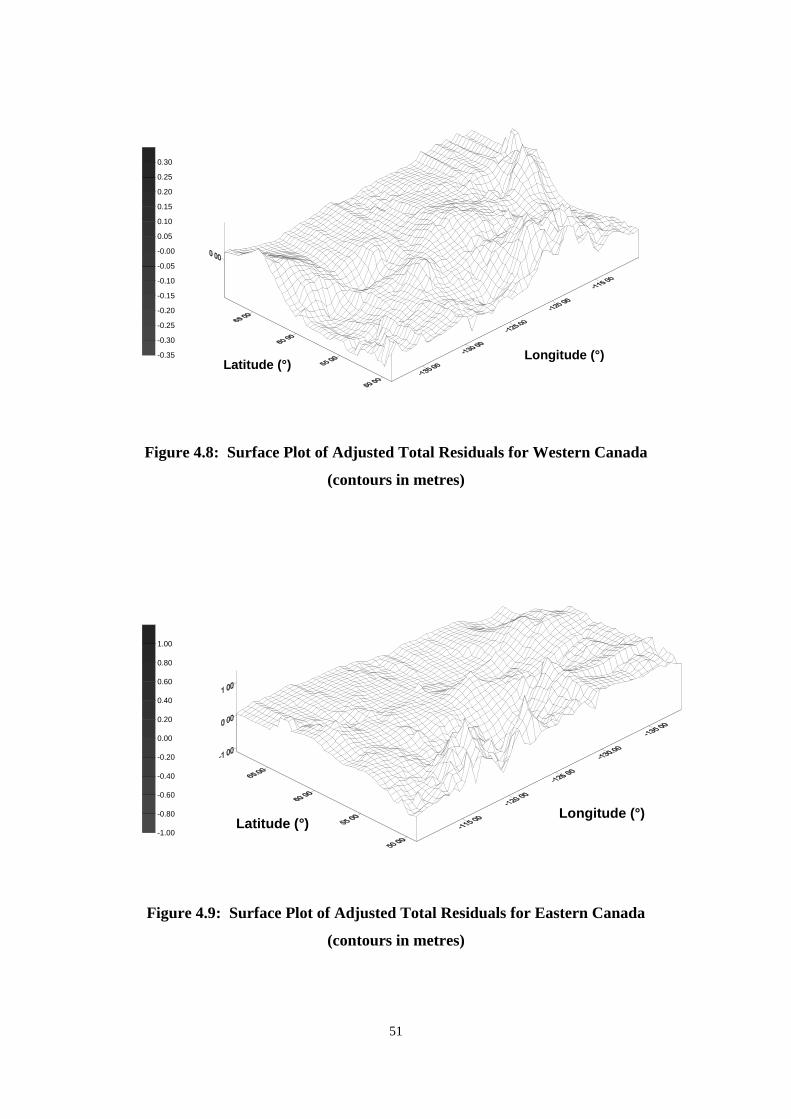
51
Figure 4.8: Surface Plot of Adjusted Total Residuals for Western Canada
(contours in metres)
Figure 4.9: Surface Plot of Adjusted Total Residuals for Eastern Canada
(contours in metres)
-0.35
-0.30
-0.25
-0.20
-0.15
-0.10
-0.05
-0.00
0.05
0.10
0.15
0.20
0.25
0.30
Longitude (°)Latitude (°)
Longitude (°)Latitude (°)
-1.00
-0.80
-0.60
-0.40
-0.20
0.00
0.20
0.40
0.60
0.80
1.00
52
4.6 A ‘Collocation’ Approach
The main disadvantage of the previous adjustment approach is the difficulty to find a
good parametric model Ax to describe all the possible systematic inconsistencies in the
height data sets (too many effects to model). This, in turn, causes problems with respect
to how reliable the results would be for the GPS/levelling/geoid noise residuals and for
the corresponding variance components. The use of classical statistical testing may help
to identify, to some degree, the weaknesses of a specific parametric model, but it cannot
provide the means for model improvement. It should be noted that a good parametric
model does not necessarily imply small values for the estimated residuals vBˆ , since the
noise level in the original height data (Qh, QH, QN) may allow relatively large values. It is
the accuracy xC ˆ of the adjusted model parameters that should determine how good a
model is, and how effectively it can be further used in future GPS/levelling applications.
Although the parameterization of the distortion effects in combined GLG networks is a
very interesting topic on its own, it may be more appropriate not to try putting all the
systematic errors in a pre-selected parametric form. For small networks, in particular, this
should be the guiding rule, since in such cases only a small number of unknown
parameters can be introduced in order to keep the degrees of freedom relatively large and
the reliability of the adjustment results relatively high. Such a ‘compact’ model is of
course unable to fully describe the complexity of the systematic effects and should be
accompanied by additional residual corrections, which were previously introduced in the
form of signals s (see equation 4.16). The solution of the general adjustment model in
Box (4.1) requires the incorporation of the signals s in the minimization principle, which
now takes the form
min 1T1T1T1T =+++ −−−−NNNHHHhhhs vQvvQvvQvsQs (4.24)
with 1−sQ being an appropriate weight matrix for the unknown correction signals.
53
Although the solution obtained by using equation (4.24) does not necessarily have to
admit a stochastic interpretation for the signal part, it is useful to consider the signals as
additional stochastic parameters, just like the zero-mean random errors v; an excellent
discussion on this aspect can be found in Dermanis (1984). The stochasticity of s is
actually necessary in the case where statistical tests related to the validity of their
weighting (covariance) model sQ are to be applied.
One of the main difficulties in this approach is that the mean value }E{sm =s of the
stochastic signals will not necessarily be zero, due to the systematic behavior that is
supposed to exist in their values. As a result, ms should appear in the final estimation
formulas if we are seeking unbiased estimators (i.e., equivalence between the least-
squares principle (4.24) and the Best Linear Unbiased Estimation-BLUE for E{s}≠0; for
detailed formulas see, e.g., Dermanis, 1987). In order to avoid such computationally
useless estimates, we can initially solve the system BvsAxl ++= using equation (4.24)
with a unit signal weight matrix. The initial solution for the signal part
( ) 1T11T )( )( −−− ++++++−= mNHhmNHhm IQQQAAIQQQAAIW (4.25a)
lWIQQQs )( ˆ 1−+++= mNHhinit (4.25b)
can be viewed as the ‘smoothest’ residual correction field, that best fits the available
observations l , the selected parametric model Ax , and the associated stochastic model
for the random noise effects (Qh, QH, QN).
Now, we can easily compute the overall trend in the signals s by fitting some very
smooth surface to the inits values. If we evaluate this fitted surface at the test network
points, we get in general some values initsms ˆˆ ≠ . We can then create the following
‘reduced’ observations and signals:
54
l l m sr = − $ (4.26a)
s s msr = − $ (4.26b)
It is now safe to assume that the reduced signals sr have zero mean, i.e., E{sr}=0.
Furthermore, the numerical values )ˆˆ( sms −init can be used for an empirical
determination of a covariance function model describing the average spatial behavior of
the reduced signals sr. In this way, we can repeat the adjustment of the model in Box
(4.1), using a new ‘improved’ version for the stochastic model of the correction signals:
BvsAxl ++= rr (4.27a)
{ }E s 0r = , { }rrr sssrr QCss E 2T σ== (4.27b)
The elements of the co-factor matrix rsQ are computed according to the empirical CV
model estimated at the previous step. An unknown variance component has been also
introduced in order to diagnose any problems related to the validity of the empirical
signal covariance function. The solution of the adjustment model in equation (4.27) will
be given by the following unbiased estimators:
( ) 1T11T )( )( −−− ++++++−=rr sNHhsNHhm QQQQAAQQQQAAIW (4.28a)
[ ] rsNHhsNHh rrlQQQQAAQQQQAx )( )( ˆ 1T11T −−− ++++++= (4.28b)
rsNHhhh rlWQQQQQv )( ˆ 1−+++= (4.28c)
rsNHhHH rlWQQQQQv )( ˆ 1−+++−= (4.28d)
55
rsNHhNN rlWQQQQQv )( ˆ 1−+++−= (4.28e)
rsNHhsr rlWQQQQQs )( ˆ 1−+++= (4.28f)
The final solution equations are similar to the ones obtained under the deterministic
approach, with the only differences being (i) the use of reduced observations lr instead of
the original l, and (ii) the incorporation of the signal covariance matrix rsQ . In the
special case of stationary white noise in all three height data sets, no significant
simplification of the above formulas occurs due to the appearance of the matrix rsQ .
The estimation of the four unknown variance components $σh2 , $σH
2 , $σ N2 , 2ˆ
rsσ follows a
straightforward extension of the MINQUE algorithm (4.23) and it is omitted.
As was mentioned previously, various statistical tests and iterative solutions can be
performed in order to finally validate the adjustment results. For statistical testing
procedures in extended adjustment models with signals, see Dermanis and Rossikopoulos
(1991) and the references given therein. In any case, a complete answer for the estimated
corrector surface should include: (i) the estimated parametric model Ax$ , (ii) the
parameters describing the non-zero mean signal trend ( $m s are just the values of this
trend at the test network points), (iii) the estimated values for the reduced zero-mean
signals $s r at the network points, and (iv) a covariance model for the zero-mean signals
s r . A combined use of (iii) and (iv), in a collocation-type prediction formula, is required
for the prediction of the zero-mean part of the correction signal at other non-levelled
points. A general flowchart for the whole computational procedure described in this
section is given in Figures (4.10a) and (4.10b).
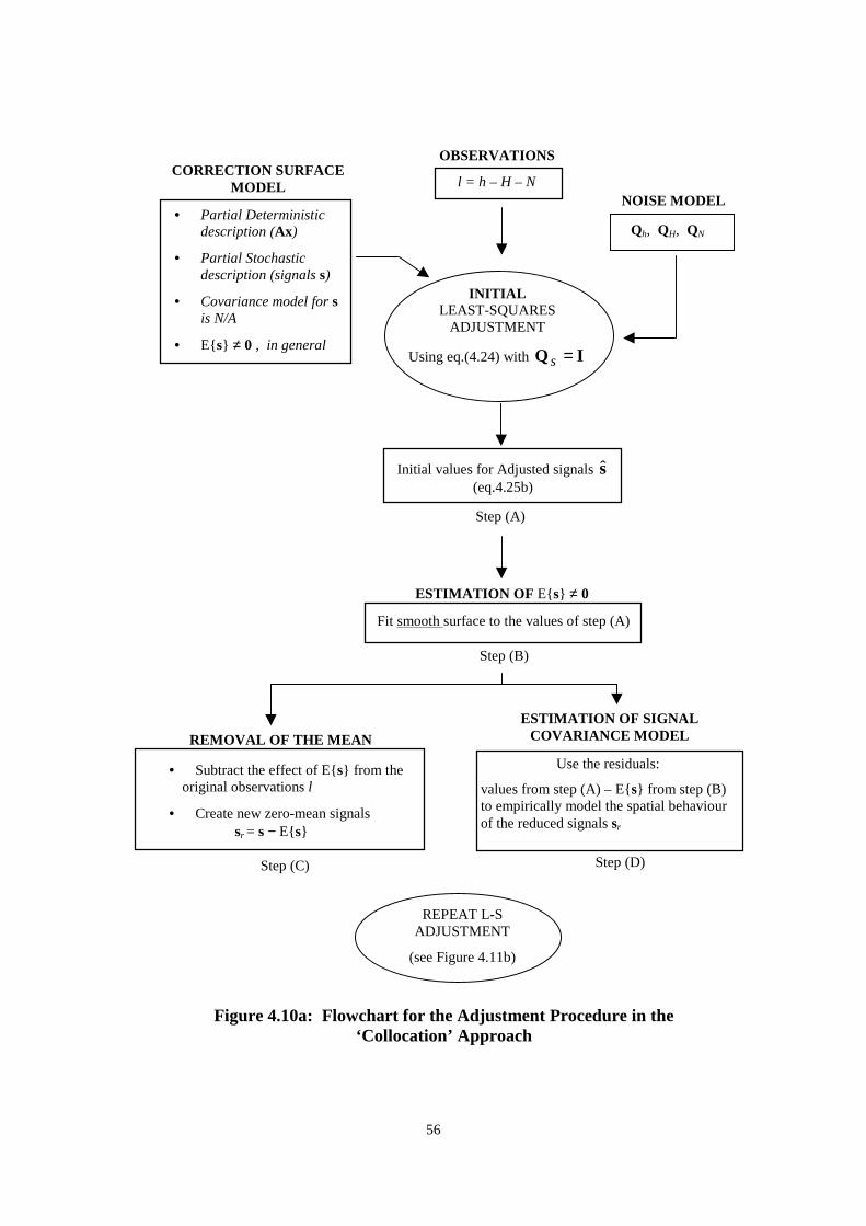
56
Figure 4.10a: Flowchart for the Adjustment Procedure in the‘Collocation’ Approach
OBSERVATIONS
l = h – H – N NOISE MODEL
Qh, QH, QN
CORRECTION SURFACEMODEL
• Partial Deterministicdescription (Ax)
• Partial Stochasticdescription (signals s)
• Covariance model for sis N/A
• E{s} ≠ 0 , in general
INITIALLEAST-SQUARES
ADJUSTMENT
Using eq.(4.24) with IQ =s
Initial values for Adjusted signals s(eq.4.25b)
Step (A)
ESTIMATION OF E{s} ≠ 0
Fit smooth surface to the values of step (A)
Step (B)
REMOVAL OF THE MEAN
• Subtract the effect of E{s} from theoriginal observations l
• Create new zero-mean signals sr = s − E{s}
Step (C)
ESTIMATION OF SIGNALCOVARIANCE MODEL
Use the residuals:
values from step (A) – E{s} from step (B)to empirically model the spatial behaviourof the reduced signals sr
Step (D)
REPEAT L-SADJUSTMENT
(see Figure 4.11b)
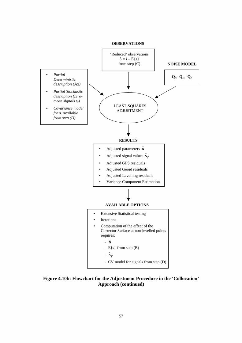
57
Figure 4.10b: Flowchart for the Adjustment Procedure in the ‘Collocation’Approach (continued)
OBSERVATIONS
‘Reduced’ observationslr = l – E{s}from step (C) NOISE MODEL
Qh, QH, QN• Partial
Deterministicdescription (Ax)
• Partial Stochasticdescription (zero-mean signals sr)
• Covariance modelfor sr availablefrom step (D)
LEAST-SQUARESADJUSTMENT
RESULTS
• Adjusted parameters x
• Adjusted signal values rs
• Adjusted GPS residuals
• Adjusted Geoid residuals
• Adjusted Levelling residuals
• Variance Component Estimation
AVAILABLE OPTIONS
• Extensive Statistical testing
• Iterations
• Computation of the effect of theCorrector Surface at non-levelled pointsrequires:
- x- E{s} from step (B)
- rs
- CV model for signals from step (D)
58
4.7 Statistical Testing in GPS/Levelling/Geoid Networks
Statistical testing for various (linear) types of hypotheses in the general adjustment
models considered in this study is a very extensive and important topic. Since it is
impossible to be fully covered in a single section, an attempt will only be made to draw
some general lines, particularly in conjunction with the specific applications of GLG
network adjustments. Relevant references in the geodetic literature that should be
consulted for a more in-depth treatment of the statistical testing problem in general and
extended adjustment models include Dermanis and Rossikopoulos (1991), Krakiwsky
and Biacs (1990), Persson (1982), and Wei (1987). In all these references, as in the
following discussion, all the stochastic components of the adjustment model (noise,
signals) are assumed to be Gaussian distributed vectors of random variables.
The inherent peculiarity of GLG networks, compared to classical 1D, 2D, 3D, or
integrated 1D/2D/3D geodetic networks, is a relatively high level of uncertainty
regarding the validity of almost every component in the adjustment model. In most
classical geodetic network problems, little doubt exists about the selected parametric
models and the observational noise stochastic model, which are trusted to describe
physical reality in a very consistent manner. In integrated geodetic networks, also, the
necessary covariance model for the signal part can be very reliably determined by
processing ‘external’ data (e.g., gravity anomalies, deflections of the vertical, etc.). The
situation is different, however, in GLG networks where the complexity of the systematic
effects involved, the often questionable gravimetric geoid error modeling, and the
absence of any external information for determining a good statistical model for the
residual correction signals, cause serious problems in the selection of realistic parametric,
signal, and observational noise models. As a result, statistical testing in this kind of
networks should not be viewed just as a ‘luxury’ for identifying possible outliers in the
original observations, but rather as a necessity for validating and testing both the a-priori
information and the modelling choices.
59
Before any special tests are performed for checking particular features of the general
adjustment model, some global statistical test must be used first. This test will indicate if
the overall model is problematic, without identifying in which specific part (parameters,
signal, noise). For this type of test, the employed test statistic is
u f T= −$ $ ~e M e1 2χ (4.29)
where $ $ $ $ $e v v v s= − − +h H N r , M Q Q Q Q= + + +h H N s , and f are the degrees of
freedom. In case where a fully deterministic approach has been followed for the GLG
network adjustment, the terms corresponding to the signal part should be omitted from
the statistic u. The acceptance of the test, for some adopted level of significance a, is
verified if χ χα αf fu2 1 2 2 2( / ) ( / )− ≤ ≤ .
The previous test gives an overall impression of the model validity but further testing is
always required since it is possible that effects from different modelling errors cancel
each other out in the computation of u. The next series of tests to be traditionally carried
out are those for individual outliers in the observations, using data snooping. They are
well documented in the geodetic literature, following Baarda’s pioneering work. Such
tests are not discussed here, their usefulness however should be always exploited after
having eliminated all possible modelling errors.
Tests on the validity of the stochastic model for the observational height data noise, and
on the admissibility of the empirical covariance model for the correction signals, require
the estimation of the corresponding unknown variance components. A general hypothesis
for variance components is (Rao and Kleffe, 1988)
H : vs. H : o aH d H dσ σ= ≠ (4.30)
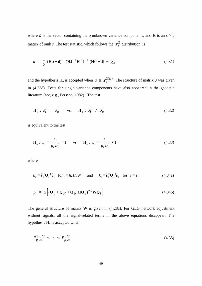
60
where σ is the vector containing the q unknown variance components, and H is an s × q
matrix of rank s. The test statistic, which follows the χs2 distribution, is
u s 1
2 ( ) ( ) ( ) ~ T T 2= − −− −H d HJ H H d$ $σ σ1 1 χ (4.31)
and the hypothesis Ho is accepted when u s ≤ χ α2( ) . The structure of matrix J was given
in (4.23d). Tests for single variance components have also appeared in the geodetic
literature (see, e.g., Persson, 1982). The test
H : vs. H : o aσ σ σ σi o i o2 2 2 2= ≠ (4.32)
is equivalent to the test
1
: H vs.1
: H2a2o ≠===oi
ii
oi
ii p
ku
p
ku
σσ (4.33)
where
r1T1T for ˆˆ and ,,for ˆˆ sikNHhik rsriiiii ==== −− sQsvQv (4.34a)
[ ]pi h H N s i tr ( + + )= + −Q Q Q Q WQ1 (4.34b)
The general structure of matrix W is given in (4.28a). For GLG network adjustment
without signals, all the signal-related terms in the above equations disappear. The
hypothesis Ho is accepted when
F u Fpa
i pa
i i,/
,/
∞−
∞≤ ≤1 2 2 (4.35)
61
where F denotes centennial points of the Fisher distribution.
Another important family of statistical tests can be used to check the performance of the
deterministic model for the systematic distortion effects in GLG networks. Although it
would be very useful to be able to test between different deterministic model choices, no
statistical tools are available in this direction. The only possibility is to compare ‘nested’
deterministic models, which essentially means to either test for the existence of possible
additional parameters in an already adopted model (model expansion) or to test the
possibility of deleting some of the already used model parameters (model shrinkage).
Computationally efficient statistics have been developed for performing the above tests,
which do not require the repetition of the adjustment procedure using the
expanded/shrinked parametric model. All the necessary formulas can be found in
Dermanis and Rossikopoulos (1991). An additional empirical tool that can be employed
for a rough check of the deterministic model is the use of correlation values among the
adjusted model parameters. High correlation suggests possible over-parameterization,
whereas low correlation gives priority to model expansion.
A combined use of all the above mentioned tests, with parallel iterative adjustment
solutions incorporating at each step in the stochastic model the previously estimated
variance components and probably correcting the deterministic model, should be
employed for a rigorous assessment of GLG networks. It is likely that after some
iterations the variance components will be stabilized to some certain values. If, in
addition, the accuracy of the adjusted model parameters is satisfactory, we can then trust
the final results to contain valuable information regarding the actual gravimetric geoid
noise level, and the behavior of the systematic effects that are needed to transform GPS
heights to orthometric heights relative to the local vertical datum.
One final important comment should be made for the covariance model of the correction
signals sr. Apart from the straightforward empirical way of computing such a preliminary
covariance model (as it was described in a previous section) and assigning a single
variance component for controlling its validity, there is always the alternative to use an a-
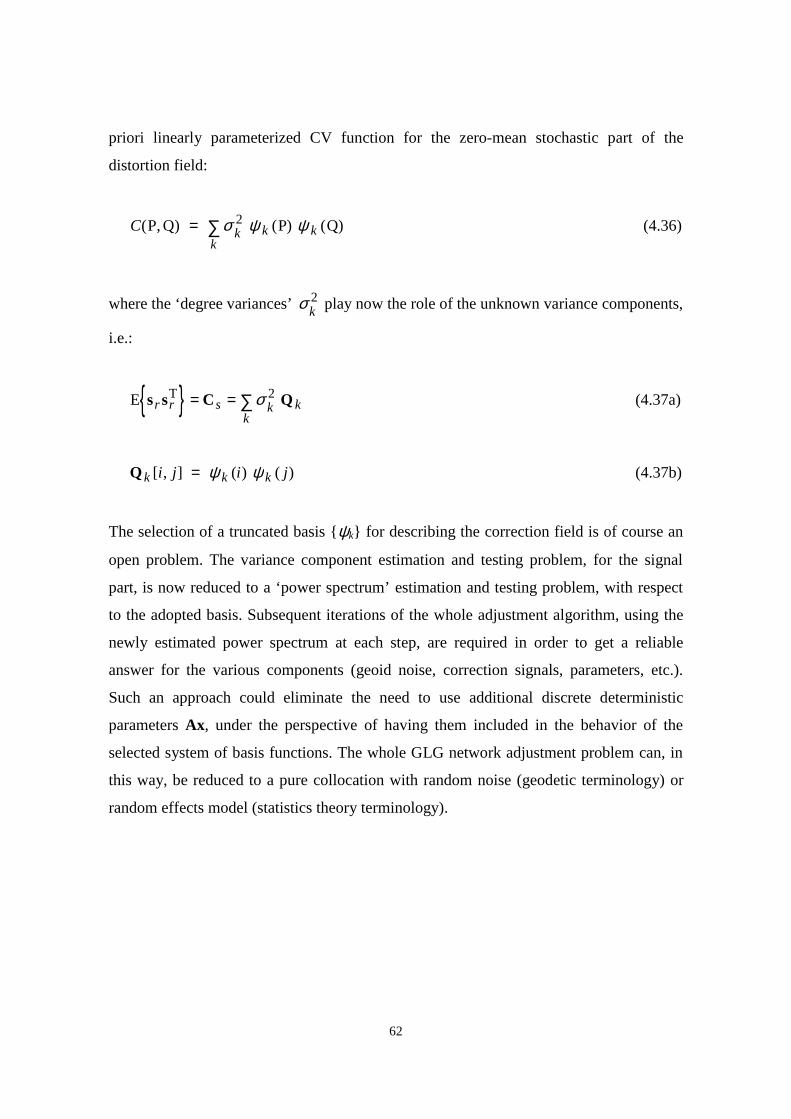
62
priori linearly parameterized CV function for the zero-mean stochastic part of the
distortion field:
C k k kk
( ) ( ) ( )P, Q P Q= ∑σ ψ ψ2 (4.36)
where the ‘degree variances’ σk2 play now the role of the unknown variance components,
i.e.:
{ }E Ts s C Qr r s k kk
= = ∑σ 2 (4.37a)
Q k k ki j i j[ , ] ( ) ( ) = ψ ψ (4.37b)
The selection of a truncated basis {ψk} for describing the correction field is of course an
open problem. The variance component estimation and testing problem, for the signal
part, is now reduced to a ‘power spectrum’ estimation and testing problem, with respect
to the adopted basis. Subsequent iterations of the whole adjustment algorithm, using the
newly estimated power spectrum at each step, are required in order to get a reliable
answer for the various components (geoid noise, correction signals, parameters, etc.).
Such an approach could eliminate the need to use additional discrete deterministic
parameters Ax, under the perspective of having them included in the behavior of the
selected system of basis functions. The whole GLG network adjustment problem can, in
this way, be reduced to a pure collocation with random noise (geodetic terminology) or
random effects model (statistics theory terminology).
63
5. Concluding Remarks
A new geoid model (GARR98) has been computed for Canada and parts of the United
States by using the EGM96 global geopotential model and local surface and marine
gravity data. Terrain effects were modeled through the use of a 1 km × 1 km DEM for all
of western Canada. The overall agreement of GARR98 with the GPS/levelling data is
approximately 14 cm, after datum inconsistencies have been removed via the four-
parameter transformation and outliers have been eliminated from the original
GPS/levelling data. This overall accuracy approximately agrees with GSD95, however
differences between the two geoid models were observed when a regional analysis was
applied. Also, before the four-parameter transformation was applied at the GPS
benchmarks, GARR98 improved the standard deviation obtained by GSD95 by more than
100% (from 44 cm to 20cm).
The similar accuracy results between western and eastern Canada (for both GARR98 and
GSD95) indicated that the strong terrain effects in the western mountainous areas were
properly modelled in both geoid models. The highest level of agreement for all models is
achieved in central Canada ranging from 9 cm to 6 cm for GARR98 and GSD95,
respectively. For all of Canada, the two global geopotential models show similar relative
accuracies up to baseline lengths of 350 km, ranging from 3.5 ppm to 0.5 ppm. In Eastern
Canada, OSU91A shows slightly better relative accuracies than EGM96 for baseline
lengths up to 400 km, whereas EGM96 has better overall accuracy especially in the
western regions giving relative accuracies better than 1 ppm for baselines greater than
200 km.
The main differences between GARR98 and GSD95 can be attributed to the additional
gravity and height data that were used in the GSD95 solution for parts of Eastern Canada
(see section 2.1). This demonstrates the importance of incorporating extended gravity and
height information in gravimetric geoid solutions for large areas, such as Canada, in order
to achieve the level of accuracy required for substituting conventional spirit levelling by
GPS techniques. In addition, advances in global geoid modelling through the inclusion of
64
EGM96 help towards meeting the requirements for a more accurate national geoid model.
Given these improvements in terms of data and the results from our kinematic DGPS
campaign, it is evident that combining GPS with an accurate geoid model may be an
efficient and accurate alternative to the traditional spirit levelling techniques currently
being used.
The use of combined GPS/Levelling/Geoid networks provides a very attractive
evaluation scheme for the accuracy of gravimetric geoid models. At the same time, GLG
networks constitute the skeleton of ‘common points’ in the attempt to find optimal
transformation models between GPS and orthometric heights. These are two different
problems which, nevertheless, can be attacked simultaneously through a unified
adjustment setting. As far as the geoid evaluation problem is concerned, a GLG network
adjustment can essentially be used for testing the reliability of preliminary internal geoid
error models, which have been derived via error propagation from the source data and
their noise used in the gravimetric solution. Variance component estimation has been
proposed as a useful statistical tool for computing and testing the actual geoid noise level.
The important role played by the stochastic noise model of the other two height
components was also demonstrated through the derived filtering equations for the total
noise residuals of the adjustment. This general approach also allows us to check
individually various additive geoid error models (see comment at the end of Section 4.2).
In the absence of any prior geoid error model, we can still use a unit weight matrix and
get an estimate for the a-posteriori unit geoid variance.
For the problem of modeling a corrector surface for GPS-to-orthometric height
transformation, it is important to filter out all the zero-mean random noise effects coming
from the triplet of the height data. This is the main weakness of some of the presently
available attempts for such a modelling. This correction surface will also absorb a part of
the geoid long-wavelength error which does not necessarily follow a zero-mean random
behavior, and it is not possible to be explicitly isolated. Two modeling alternatives have
been presented for the description of the systematic correction field. These included: (a)
purely discrete deterministic modelling, (b) hybrid deterministic and ‘stochastic’
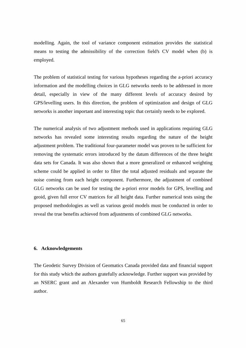
65
modelling. Again, the tool of variance component estimation provides the statistical
means to testing the admissibility of the correction field’s CV model when (b) is
employed.
The problem of statistical testing for various hypotheses regarding the a-priori accuracy
information and the modelling choices in GLG networks needs to be addressed in more
detail, especially in view of the many different levels of accuracy desired by
GPS/levelling users. In this direction, the problem of optimization and design of GLG
networks is another important and interesting topic that certainly needs to be explored.
The numerical analysis of two adjustment methods used in applications requiring GLG
networks has revealed some interesting results regarding the nature of the height
adjustment problem. The traditional four-parameter model was proven to be sufficient for
removing the systematic errors introduced by the datum differences of the three height
data sets for Canada. It was also shown that a more generalized or enhanced weighting
scheme could be applied in order to filter the total adjusted residuals and separate the
noise coming from each height component. Furthermore, the adjustment of combined
GLG networks can be used for testing the a-priori error models for GPS, levelling and
geoid, given full error CV matrices for all height data. Further numerical tests using the
proposed methodologies as well as various geoid models must be conducted in order to
reveal the true benefits achieved from adjustments of combined GLG networks.
6. Acknowledgements
The Geodetic Survey Division of Geomatics Canada provided data and financial support
for this study which the authors gratefully acknowledge. Further support was provided by
an NSERC grant and an Alexander von Humboldt Research Fellowship to the third
author.
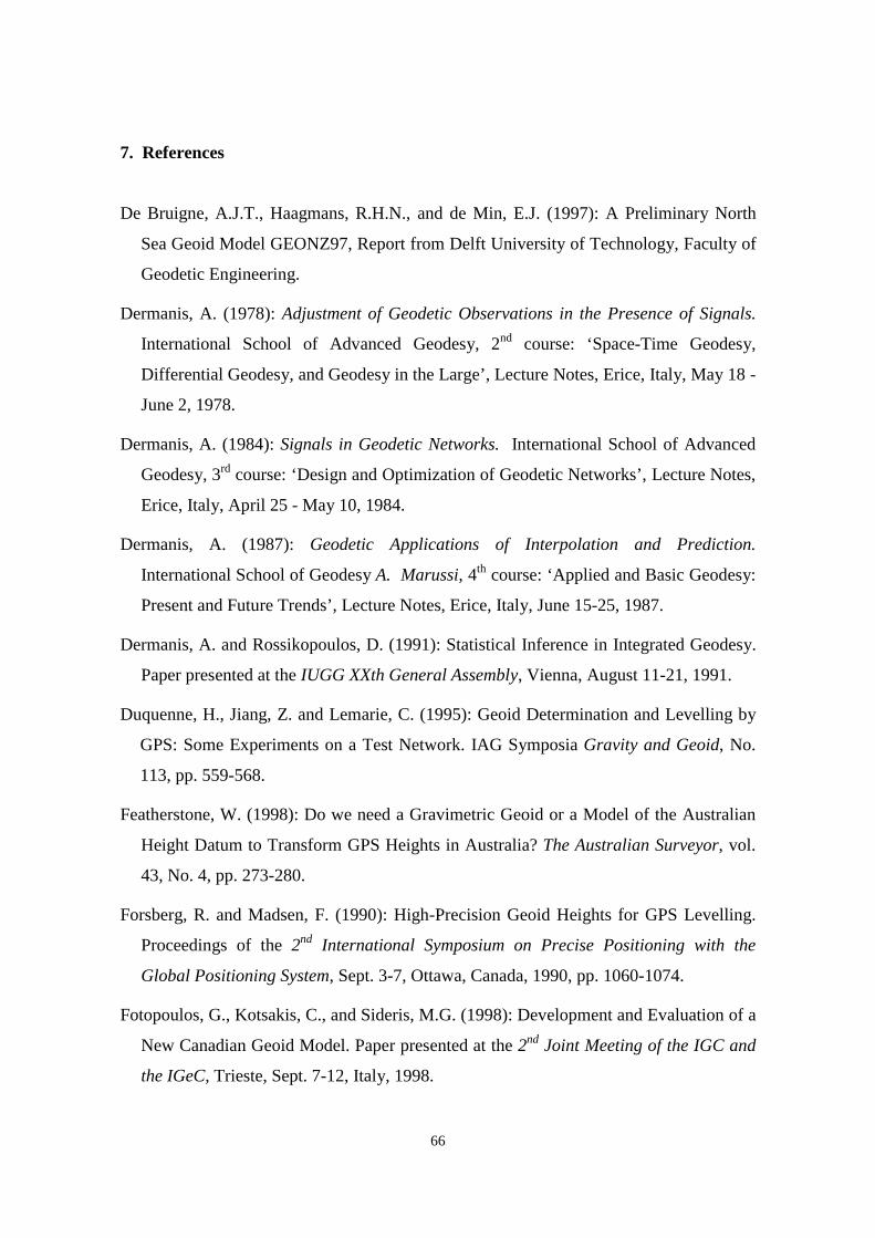
66
7. References
De Bruigne, A.J.T., Haagmans, R.H.N., and de Min, E.J. (1997): A Preliminary North
Sea Geoid Model GEONZ97, Report from Delft University of Technology, Faculty of
Geodetic Engineering.
Dermanis, A. (1978): Adjustment of Geodetic Observations in the Presence of Signals.
International School of Advanced Geodesy, 2nd course: ‘Space-Time Geodesy,
Differential Geodesy, and Geodesy in the Large’, Lecture Notes, Erice, Italy, May 18 -
June 2, 1978.
Dermanis, A. (1984): Signals in Geodetic Networks. International School of Advanced
Geodesy, 3rd course: ‘Design and Optimization of Geodetic Networks’, Lecture Notes,
Erice, Italy, April 25 - May 10, 1984.
Dermanis, A. (1987): Geodetic Applications of Interpolation and Prediction.
International School of Geodesy A. Marussi, 4th course: ‘Applied and Basic Geodesy:
Present and Future Trends’, Lecture Notes, Erice, Italy, June 15-25, 1987.
Dermanis, A. and Rossikopoulos, D. (1991): Statistical Inference in Integrated Geodesy.
Paper presented at the IUGG XXth General Assembly, Vienna, August 11-21, 1991.
Duquenne, H., Jiang, Z. and Lemarie, C. (1995): Geoid Determination and Levelling by
GPS: Some Experiments on a Test Network. IAG Symposia Gravity and Geoid, No.
113, pp. 559-568.
Featherstone, W. (1998): Do we need a Gravimetric Geoid or a Model of the Australian
Height Datum to Transform GPS Heights in Australia? The Australian Surveyor, vol.
43, No. 4, pp. 273-280.
Forsberg, R. and Madsen, F. (1990): High-Precision Geoid Heights for GPS Levelling.
Proceedings of the 2nd International Symposium on Precise Positioning with the
Global Positioning System, Sept. 3-7, Ottawa, Canada, 1990, pp. 1060-1074.
Fotopoulos, G., Kotsakis, C., and Sideris, M.G. (1998): Development and Evaluation of a
New Canadian Geoid Model. Paper presented at the 2nd Joint Meeting of the IGC and
the IGeC, Trieste, Sept. 7-12, Italy, 1998.
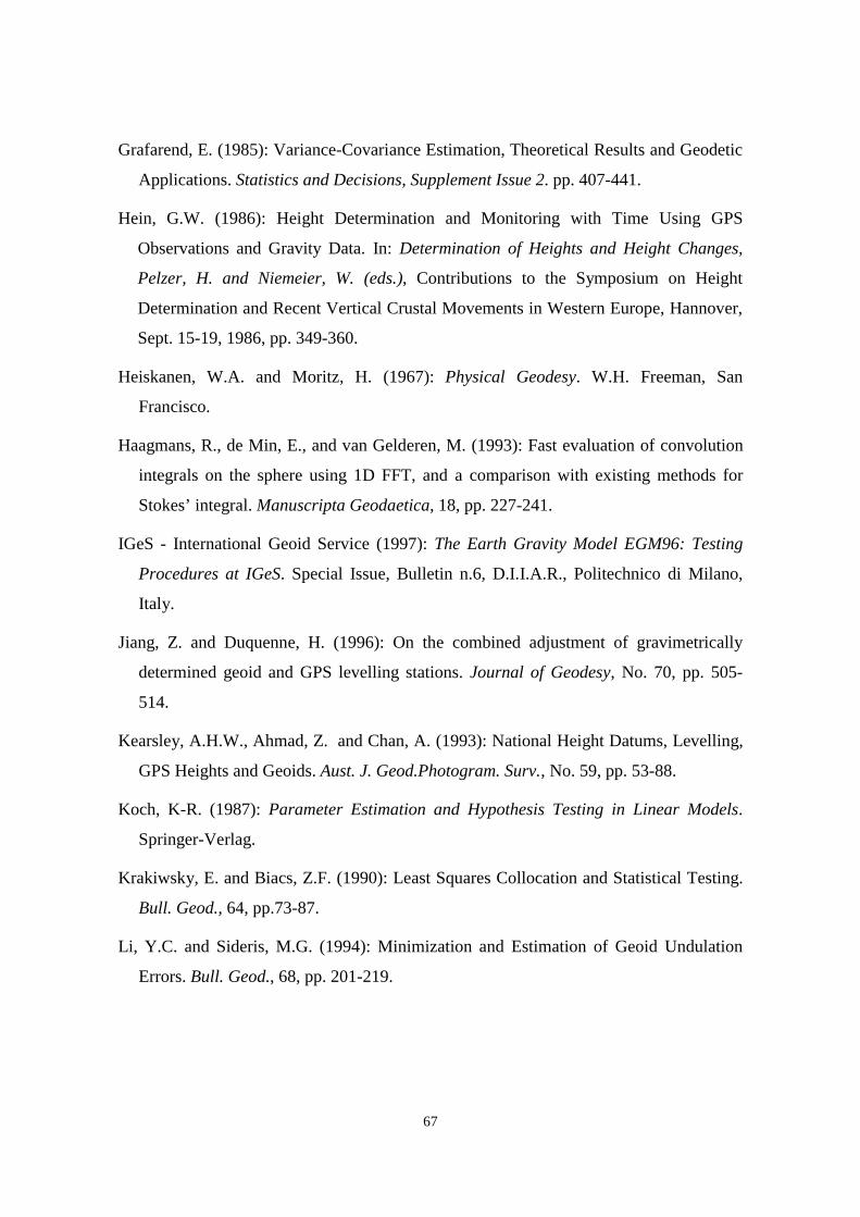
67
Grafarend, E. (1985): Variance-Covariance Estimation, Theoretical Results and Geodetic
Applications. Statistics and Decisions, Supplement Issue 2. pp. 407-441.
Hein, G.W. (1986): Height Determination and Monitoring with Time Using GPS
Observations and Gravity Data. In: Determination of Heights and Height Changes,
Pelzer, H. and Niemeier, W. (eds.), Contributions to the Symposium on Height
Determination and Recent Vertical Crustal Movements in Western Europe, Hannover,
Sept. 15-19, 1986, pp. 349-360.
Heiskanen, W.A. and Moritz, H. (1967): Physical Geodesy. W.H. Freeman, San
Francisco.
Haagmans, R., de Min, E., and van Gelderen, M. (1993): Fast evaluation of convolution
integrals on the sphere using 1D FFT, and a comparison with existing methods for
Stokes’ integral. Manuscripta Geodaetica, 18, pp. 227-241.
IGeS - International Geoid Service (1997): The Earth Gravity Model EGM96: Testing
Procedures at IGeS. Special Issue, Bulletin n.6, D.I.I.A.R., Politechnico di Milano,
Italy.
Jiang, Z. and Duquenne, H. (1996): On the combined adjustment of gravimetrically
determined geoid and GPS levelling stations. Journal of Geodesy, No. 70, pp. 505-
514.
Kearsley, A.H.W., Ahmad, Z. and Chan, A. (1993): National Height Datums, Levelling,
GPS Heights and Geoids. Aust. J. Geod.Photogram. Surv., No. 59, pp. 53-88.
Koch, K-R. (1987): Parameter Estimation and Hypothesis Testing in Linear Models.
Springer-Verlag.
Krakiwsky, E. and Biacs, Z.F. (1990): Least Squares Collocation and Statistical Testing.
Bull. Geod., 64, pp.73-87.
Li, Y.C. and Sideris, M.G. (1994): Minimization and Estimation of Geoid Undulation
Errors. Bull. Geod., 68, pp. 201-219.
68
Mainville, A., Forsberg, R., and Sideris, M.G. (1992): Global Positioning System Testing
of Geoids Computed from Geopotential Models and Local Gravity Data: A Case
Study. Journal of Geophysical Research, vol. 97, No. B7, pp. 11,137-11,147.
Mainville, A., Veronneau, M., Forsberg, R. and Sideris, M.G. (1994): A Comparison of
Terrain Reduction Methods in Rough Topography. Paper presented at the Joint
Meeting of the International Gravity Commission and the International Geoid
Commission, Graz, Austria, 1994.
Mainville, A., Craymer, M., and Blackie, S. (1997): The GPS Height Transformation
1997, An Ellipsoidal-Orthometric Height Transformation for Use with GPS in
Canada. Report of Geodetic Survey Division, Geomatics Canada, Ottawa.
Moritz, H. (1980): Advanced Physical Geodesy. Herbert Wichmann Verlag, Karlsruhe.
Pelzer, H. (1986): Height Determination – Adjustment Models for Combined Data Sets.
In: Determination of Heights and Height Changes, Pelzer, H. and Niemeier, W.
(eds.), Contributions to the Symposium on Height Determination and Recent Vertical
Crustal Movements in Western Europe, Hannover, Sept. 15-19, 1986, pp. 327-340.
Persson, C.G. (1982): Adjustment, Weight-Testing and Detection of Outliers in Mixed
SFF-SFS Models. Manuscr. Geod., 7, pp.299-323.
Rao, C.R. (1971): Estimation of Variance Components - MINQUE Theory. Journal of
Multivariate Statistics. vol. 1, pp. 257-275.
Rao, C.R. and Kleffe, J. (1988): Estimation of Variance Components and Applications.
North-Holland Series in Statistics and Probability, vol.3.
Rao, P.S.R.S. (1997): Variance Components Estimation: Mixed Models, Methodologies,
and Applications. Monographs on Statistics and Applied Probability, vol. 78,
Chapman & Hall.
Sideris, M.G. (1990): Rigorous gravimetric terrain modelling using Molodensky's
operator. Manuscr. Geod., 15, pp. 97-106.
69
Sideris, M.G., Mainville, A., and Forsberg, R. (1992): Geoid Testing Using GPS and
Levelling (or GPS Testing Using Levelling and the Geoid?). Aust. J. Geod.
Photogram. Surv., No.57, pp. 62-77.
Sjoberg, L. (1984): Non-negative Variance Component Estimation in the Gauss-Helmert
Adjustment Model. Manuscr. Geod., 9, pp. 247-280.
Smith, D.A. and Milbert, D.G. (1996): The GEOID96 High Resolution Geoid Height
Model for the United States. National Oceanic and Atmospheric Administration
(NOAA), U.S. National Geodetic Survey, Silver Springs, MD.
9DQLþHN�� 3�� �������� 9HUWLFDO� 'DWXP� DQG� 1$9'���� Surveying and Land Information
Systems, Vol. 51, No. 2, pp. 83-86.
Veronneau, M. (1994): Determination of Mean Helmert Gravity Anomalies in a Plane
Approximation. Internal Report. Geodetic Survey Division, Geomatics Canada, Dept.
of Natural Resources Canada, Ottawa, Ontario.
Veronneau, M. (1995): An Analysis of the Gravity Measurements Used in the
Determination of the 1995 Canadian Geoid Model. Internal Report. Geodetic Survey
Division, Geomatics Canada, Dept. of Natural Resources Canada, Ottawa, Ontario.
Veronneau, M. (1996): Canadian Geoid Model GSD95 and its Precision. Internal Report.
Geodetic Survey Division, Geomatics Canada, Dept. of Natural Resources Canada,
Ottawa, Ontario.
Wei, M. (1987): Statistical Problems in Collocation. Manuscr. Geod.,12, pp. 282-289.
Wichiencharoen, C. (1982): The Indirect Effect on the Computation of Geoidal
Undulations. Report No.336, Dept. of Geodetic Science and Surveying, Ohio State
University, Columbus, Ohio.