Screening for Mice that Remember Incorrectlyruccs.rutgers.edu/images/personal-charles-r-gallistel/publications... · Screening for Mice that Remember Incorrectly Adam Philip King1

International Journal of Comparative Psychology, 2001, 14: 232-257.

Screening for Mice that Remember IncorrectlyAdam Philip King1

Fairfield UniversityRobert V. McDonaldRutgers University

C.R. GallistelRutgers University

The memory mechanism carries information forward in time. Screening for geneticdistortions in this information (screening for changes in the content of memory) is likely todo a better job of distinguishing between genetic effects on memory mechanisms and geneticeffects on performance mechanisms than screening for changes in the strength of learnedbehavior. The peak procedure is the most commonly used screen for duration memory. Micegive peak data strikingly similar to data from the rat and the pigeon. The data, however, favora model in which the decision criterion for starting the response (putting the head into thehole) and stopping the response are independently determined. For reasons we explain, thisprevents the estimation of scalar memory error and memory variability from simple peakdata.

Memory is a foundation of higher mental function, and its destruction by degenerative diseasesof the nervous system is a devastating and common health problem. Identifying the cellular andmolecular mechanisms involved in memory is essential to our understanding of these diseases.Memory mutants offer hope for rapid progress in determining these mechanisms. If we had astrain of mice that bred true for a mutation in a gene that coded for an essential component of themolecular machinery of memory, we could use the increasingly powerful techniques oftraditional and molecular genetics to locate and sequence the gene. It would then be possible touse molecular biological methods to find where and when that gene was expressed in the brain,and where the gene product was located within cells.

The identification and production of such memory mutants will depend fundamentally oneffective behavioral screens, because memory is known only by its behavioral effects. In turn,the effectiveness of behavioral screens is determined by their diagnostic specificity. Withregards to the molecular basis of memory, behavioral scientists must devise screens thatdistinguish between those genetic effects that bear directly on the mechanisms involved inmemory and those that bear on processes that translate the remembered information intoobservable behavior. These latter performance factors are numerous; they include motivation,attention, and health, as well as many factors that do not fall readily under any of these headings(Rescorla, 1998; Wilkie, Willson, & Carr, 1999). These processes affect behavioral indices ofmemory (i.e. the probability or vigor of a memory-based response), but they are functionallyindependent of the memory itself. They play no role in carrying information forward in time;they affect only the expression of that information in observable behavior.

1 Address correspondence to: Adam King, Fairfield University,North Benson Rd, Fairfield, CT06430-5195, Email: [email protected]

King, et al. Screening for mice 2

Most current behavioral screens for memory, such as the Morris water maze (e.g.,Vicens, Bernal, Carrasco, & Redolat, 1999), measure the strength of a memory-dependentbehavior and therefore potentially confound performance and memory factors. In effect, theyscreen for animals that remember poorly, or, less often, for animals that remember unusuallywell (cf. Tang et al., 1999). Measures such as latency to reach the platform do not specificallyimplicate memory as the source of variation in behavior, in that there is no simple relationshipbetween the strength of observed behavior and potential quantitative measures of the underlyingengram. It is unclear what it means, physiologically speaking, to say that a mouse remembersthe location of a platform more strongly under some circumstances than under others.

An alternative to screening for changes in the strength of memory-dependent behavior isto screen for distortions in the contents of memory, for example, 'what does a subject remembera fixed interval to be' rather than 'how likely is the subject to respond to a signal that predicts anevent that will occur at that fixed interval' (cf. Church & Meck, 1988). In a wide variety of tasks,animals remember variables like distances and durations and numerosity (Gallistel, 1990). Thisapproach to studying memory has been most extensively developed in the field of timingbehavior (Brunner, 1997; Fantino, 2000; Fetterman, 1995; Malapani, 1998; Rakitin, 1998;Roberts, 1998; Wilkie, 1995).

Among the several timing tasks that have been explored, the most thoroughly analyzedhas been the peak procedure (Catania & Reynolds, 1968; Cheng & Westwood, 1993; Cheng,Westwood, & Crystal, 1993; Church, Meck, & Gibbon, 1994; Roberts & Church, 1978). In thisprocedure, subjects indicate with their responses (e.g., key pecks or lever presses) the targetlatency, at which they expect responding will have some consequence (e.g., food delivery)following a signal event (e.g., the illumination of a key or the extension of a lever). On sometrials, the anticipated event fails to occur, in which case subjects cease responding when they nolonger anticipate it. From these probe trials one gets data reflecting the temporal interval storedin memory. Subjects begin responding somewhat before the anticipated event and ceaseresponding when they no longer expect it, thereby bracketing the time at which the event wasexpected. The advantage of using tasks like the peak procedure as a behavioral screen forchanges in the quantitative properties of memory is that the temporal distribution of responses,which reflects the information about the remembered temporal interval, is demonstrablyindependent of the strength of the behavior (Roberts, 1981). For example, a pigeon will displaythe same temporal distribution of key pecks to obtain food in both food-deprived and relativelysatiated conditions, although responding may be far more vigorous in the food-deprivedcondition. When normalized for maximum rate of pecking, these distributions will superpose.

Scalar Expectancy Theory (SET) (Gibbon, 1977, 1991; Gibbon, Church, & Meck, 1984)provides a framework that accounts for many facets of animal timing and it has been notablysuccessful in accounting for data from the peak procedure (Cheng & Westwood, 1993; Cheng etal., 1993; Church et al., 1994; Gibbon & Church, 1992; Meck & Church, 1984; Meck & Church,1987). SET makes explicit the basic operations presumably implemented in any system capableof solving the peak task (Figure 1). First, the system must have a timer (clock) that delivers anon-going measure of elapsed duration. It must have a memory, a mechanism for carrying forwardin time records of the elapsed intervals at which food has previously been delivered. Finally, itmust have a comparator to decide whether the currently elapsed interval is close enough to theremembered interval to begin responding and whether it has grown sufficiently longer than theremembered latency to terminate responding. 'Close enough’ and 'sufficiently longer' arespecified by decision criteria.


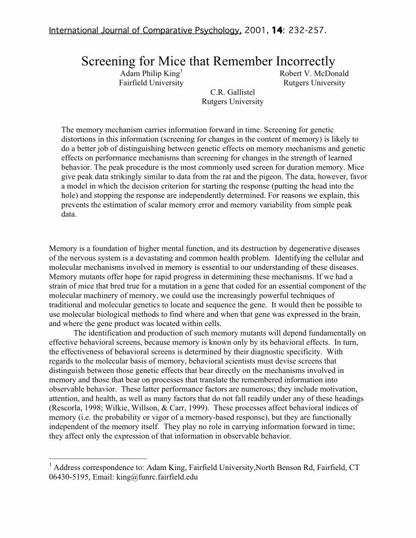
Figure 1. The SET framework. Solid arrowsrepresent variables that vary continuouslywith time (e.g., subjective time); dashedarrows represent variables that take onenduring values at specific moments in time(e.g., memories for durations). Hattedvariables are subjective quantities (notdirectly observable); variables without hatsare objective quantities (directlymeasurable). t = objective trial time; ˆ t =subjective trial time; ˆ d = the delay beforestarting the timer; ˆ s = clock speed, theslope of the function relating subjective trial time to objective trial time; T *= the target latency;ˆ k = the memory scalar ; ˆ m , a sample from memory used as the reference (or target) value on a

probe trial; ˆ l = the proportion by which the start criterion anticipates the target value; ˆ u = theproportion by which the stop criterion exceeds the target value.

Three quantitative features have been fairly well established when applying the SET frameworkto the data from the peak procedure (hereafter 'peak data’). First, the subjective measure of trialduration is proportional to objective duration (Gallistel, 1999; Gibbon & Church, 1981). Thedecision variable in SET is the ratio of the currently elapsing interval to the remembered interval(Aronson, Balsam, & Gibbon, 1993; Gibbon, 1991, 1992; Gibbon & Fairhurst, 1994). Third, themajor sources of variability scale with the remembered temporal interval.

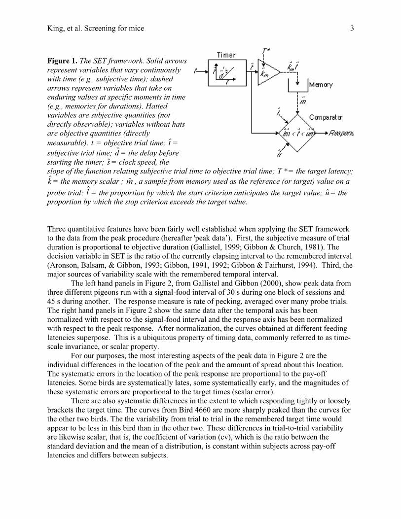
The left hand panels in Figure 2, from Gallistel and Gibbon (2000), show peak data fromthree different pigeons run with a signal-food interval of 30 s during one block of sessions and45 s during another. The response measure is rate of pecking, averaged over many probe trials.The right hand panels in Figure 2 show the same data after the temporal axis has beennormalized with respect to the signal-food interval and the response axis has been normalizedwith respect to the peak response. After normalization, the curves obtained at different feedinglatencies superpose. This is a ubiquitous property of timing data, commonly referred to as time-scale invariance, or scalar property.

For our purposes, the most interesting aspects of the peak data in Figure 2 are theindividual differences in the location of the peak and the amount of spread about this location.The systematic errors in the location of the peak response are proportional to the pay-offlatencies. Some birds are systematically lates, some systematically early, and the magnitudes ofthese systematic errors are proportional to the target times (scalar error).

There are also systematic differences in the extent to which responding tightly or looselybrackets the target time. The curves from Bird 4660 are more sharply peaked than the curves forthe other two birds. The the variability from trial to trial in the remembered target time wouldappear to be less in this bird than in the other two. These differences in trial-to-trial variabilityare likewise scalar, that is, the coefficient of variation (cv), which is the ratio between thestandard deviation and the mean of a distribution, is constant within subjects across pay-offlatencies and differs between subjects.


Figure 2. Left. Average pecking rates on probe (no-food) trials during sessions when the latency(T*) between key illumination and food delivery was either 30 s or 45 s. Each panel gives datafrom a different bird (identified by the number on the panel). The feeding latencies are indicatedby the vertical lines. Right. The same data after normalization with respect to target latency andpeak response rate. (Reproduced with slight modifications from Gallistel & Gibbon, 2000).

It is important to appreciate that between subject variations in the rates at which theirtimers run are unlikely to result in the between-subject differences in peak location seen inFigure 2. A subject with a slow timer would not be expected to have a peak located later than thetarget time, nor would a subject with a fast timer be expected to have a peak located before thetarget time. The location of the peak is determined by a comparison between two times, both ofwhich presumably come from the same timer. One time is the currently elapsing interval, andone is the remembered pay-off latency. Because both times come from the same timer, betweensubject timer differences cancel out in determining the location of the peak relative to the target.The systematic error is also unlikely to reflect a strategy peculiar to the peak procedure becausesome subjects show a positive scalar error, some show a negative scalar error, and some showalmost no scalar error (see Figure 2). While many performance factors could increase ordecrease response latencies, they should have fixed, rather than proportional, effects (i.e., theireffect should be independent of the latency remembered). The fact that the error is proportional


to the remembered latency strongly constrains the plausible source(s) for that error; it (they) mustmultiply the contents of memory.

In SET theory, these systematic errors have often been accounted for by postulating amultiplicative calibration error between the pay-off latencies as measured by the timer and thevalues that are retrieved from memory (Gibbon et al., 1984)1. Specifically, in Gibbon’s (1984)model, the memory stage delivers to the comparator a remembered target latency whoseexpectation differs from the true latency by a multiplicative factor. This factor has usually beensymbolized by K*. To be consistent with our notational conventions (Table 1A in theAppendix), we adopt the notation Km.

If memory calibration can be shown to be the primary source of the systematic scalarerrors in peak location, then between-subject variation in the memory calibration constant, Km,can be viewed as analogous to the between-subject variation in tau, the period of the circadianclock. That is, the behaviorally observed memory errors may reflect genetically derivedvariability in the underlying molecular mechanism. This could give us a means of finding therelevant genes, just as behaviorally observed genetic variation in tau has done in the case of thecircadian clock (Antoch et al., 1997; Dunlap, 1993)

The smooth rises and falls in Figure 2 are averaging artifacts. On any given peak trial,responding has the form of a square pulse, with an abrupt onset, an abrupt offset, and a steadyhigh rate during the response interval. The onset and offset times are determined by the start andstop criteria, which are approximately proportional to the target time (the remembered pay-offlatency). That is, subjects start when the elapsed time has reached a certain percentage of thetarget time and stop when it has exceeded the target time by some percentage. Asymmetry ofstart and stop proportions is another potential source of systematic error in the location of thepeak response probability. If, as has often been assumed, these proportions differ from therememberd pay-off latency by a common hedge factor (minus and plus the same percentage),then the center of the response interval is the remembered pay-off latency. If, however, theseproportions are independent of one another, then the center of the response interval need not bethe remembered pay-off latency. For the peak procedure to be a successful memory screen, it isimportant to determine if this possibility can be ruled out.

We turn now to the second aspect of the data in Figure 2 that might be a good target formemory screening, the between subject differences in trial-to-trial variability. For the scalarvariability (proportional spread) seen in the peak data, there are three potential sources. First, itis often assumed that that memory itself is a major source (Church, et al., 1994; Gibbon, 1994);the remembered pay-off latency is assumed to vary from trial to trial. Other likely sources aretrial-to-trial variability in the start and stop proportions and in trial-to-trial variability in clockspeed. Our ability to estimate the relative contributions of these sources determines the utility ofthe peak procedure as a screen for genetically controlled quantitative variation in the memorymechanism.

The successful use of the peak procedure (or similar tasks) as a behavioral screen formemory mutants depends on its application to individual subjects (group data is of little usehere) and the use of subjects amenable to genetic analysis. A great deal of work has been doneon analyzing and modeling the group performance of rats and pigeons in the peak procedure.However, little work has been done on analyzing and modeling the performance of individualsubjects. In addition, there has been little peak procedure work using mice, which offer thegreatest opportunity for genetic analysis.


In this paper, we report a variant of the peak procedure designed specifically for mice.Our main focus, however, is on the application of different analytic methods to the extractionfrom the data of estimates of the scalar memory error and memory variability, and on the closelyrelated problems of distinguishing between scalar memory error and asymmetrical decisioncriteria, and between variability due to memory and variability from other sources.

MethodSubjects

The subjects were 2 female Swiss-Webster ND4 mice (Harlan, Indianapolis IN) weighingbetween 25-26 g at the start of the experiment. Subjects were housed individually in clearshoebox cages and maintained on a 12:12 hr light/dark schedule with lights on at 0800. Alltraining took place during the dark portion of the photoperiod. Subjects were left undisturbed inthe colony room for 1 week after arrival. At the end of the first week, access to food wasrestricted and training was begun. During training, the subjects obtained 30 - 70% of their totalfood intake while in the operant chamber, and this was supplemented with 1-3 g of additionalfood at the end of each training session. The amount of supplemental food delivered dependedon the amount of food obtained during the training session, and was adjusted on a daily basis toprevent excessive weight loss. Water was available ad lib. in both the home cage and operantchamber.Apparatus

All training took place in operant chambers (Med Associates model # ENV307AW, 7 x 8x 5 in). The chambers were located in individual ventilated, sound-attenuating boxes. Eachchamber was equipped with three pellet dispensers each connected to a feeding station along onewall of the chamber. A control station (identical to the feeding stations, but not connected to apellet dispenser) was located on the opposite wall. Each station was equipped with an infraredbeam that detected nose pokes into that station, and a light that illuminated the pellet deliveryarea. The chambers were also each equipped with a tone generator (2900 Hz) and a white noisegenerator (80 db, flat 10-25,000 Hz). When activated, the pellet dispensers delivered a single 20mg food pellet (A.J. Noyes, #PJA/100020).Procedure

Subjects were weighed at the start of each session and then placed in the operantchambers. The opportunity to begin a trial was signaled by the illumination of the control stationand the onset of white noise. These stimuli remained present until the subject poked its nose intothe control station. When the poke was detected, the control station illumination and white noisewere terminated, the target feeding station was illuminated, the tone turned on, and the feedingclock started. Feeding trials were Fixed Interval trials, on which the feeder was armed when thefeeding clock reached the target latency (T*). A single pellet was delivered at T* if the beamwas interrupted at that moment; otherwise, it was delivered at the first detected interruptionfollowing T*. Illumination of the target feeding station was terminated 10 s following pelletdelivery. On trials where no nose poke was detected at or after T*, the trial ended after 3T* plusan interval chosen from an exponential distribution with an expectation of T*. Probe trials, whenno food was delivered, occurred on an average of one out of five trials. On these trials, thefeeding station remained illuminated and the tone on for an interval equal to 2T* plus an intervaldrawn from an exponential distribution with an expectation equal to T*. Following each trial,there was an ITI equal to 2T* plus a random interval chosen from an exponential distributionwith an expectation of T*. At the end of this interval, the control station was again illuminated


and the white noise turned back on, enabling the mouse to start the next trial. Sessions lasted 12hours. The number of trials in a session was controlled by the subject’s behavior, and rangedfrom 75 to 250. All aspects of the experimental protocol were controlled by computer software(Med-PC, Med Associates). The subject’s interruption of the IR beams was recorded with atemporal resolution of 20 ms.

Subjects were initially trained with a target latency of 20 s, and this protocol remained ineffect for 16 sessions. Following this, the target latency was changed to 30 s for 15 sessions andthen to 10 s for 10 sessions. For data analysis, we used all the sessions after the session at whichvisual inspection of the raster plots (see Figure 3) suggested that behavior had stabilized. ForM302, this was the last 7 sessions in each condition. For M301, it was the last 9 sessions in theT* = 20 s and 10 s conditions and the last 14 sessions in the T* = 30 s condition.

ResultsThe subject’s behavior on probe trials may be visualized by means of a raster plot in

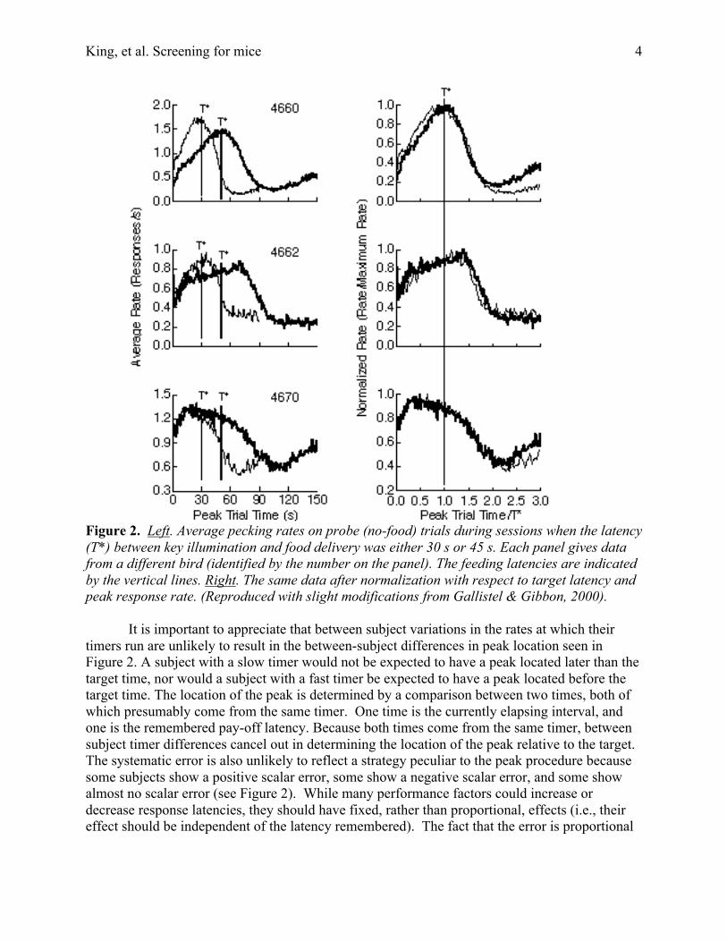
which the x-axis represents time since the beginning of a probe trial and the y-axis represents thesequence of probe trials within a session. A plotted point indicates that the subject had its headin the lit hopper at that moment (x axis) on that trial (y axis). Figure 3 shows raster plots forsubject 301 and subject 302 for their final session with a T* of 10 s and in the final session with aT* of 30 s.

Figure 3. Raster plots of head-poke behavior on probe trials in sessions with different feedinglatencies (T* = 10 s in upper panels, 30 s in lower). Each horizontal line is one trial. The times


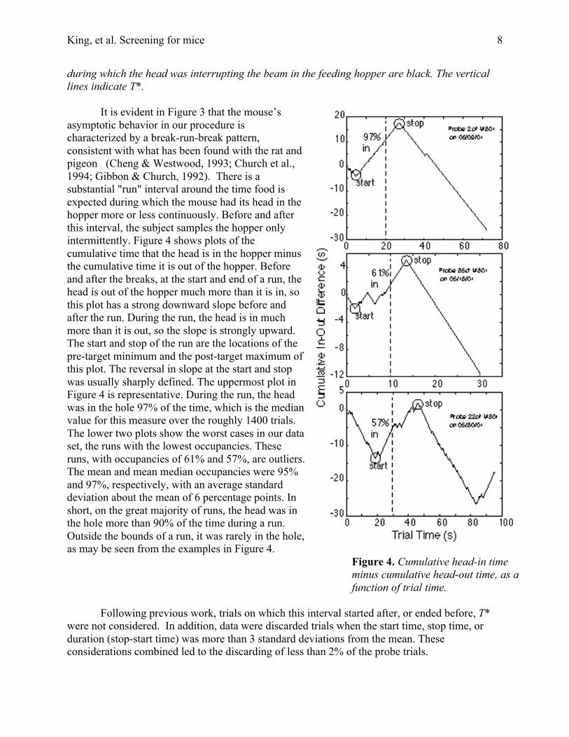
during which the head was interrupting the beam in the feeding hopper are black. The verticallines indicate T*.

It is evident in Figure 3 that the mouse’sasymptotic behavior in our procedure ischaracterized by a break-run-break pattern,consistent with what has been found with the rat andpigeon (Cheng & Westwood, 1993; Church et al.,1994; Gibbon & Church, 1992). There is asubstantial "run" interval around the time food isexpected during which the mouse had its head in thehopper more or less continuously. Before and afterthis interval, the subject samples the hopper onlyintermittently. Figure 4 shows plots of thecumulative time that the head is in the hopper minusthe cumulative time it is out of the hopper. Beforeand after the breaks, at the start and end of a run, thehead is out of the hopper much more than it is in, sothis plot has a strong downward slope before andafter the run. During the run, the head is in muchmore than it is out, so the slope is strongly upward.The start and stop of the run are the locations of thepre-target minimum and the post-target maximum ofthis plot. The reversal in slope at the start and stopwas usually sharply defined. The uppermost plot inFigure 4 is representative. During the run, the headwas in the hole 97% of the time, which is the medianvalue for this measure over the roughly 1400 trials.The lower two plots show the worst cases in our dataset, the runs with the lowest occupancies. Theseruns, with occupancies of 61% and 57%, are outliers.The mean and mean median occupancies were 95%and 97%, respectively, with an average standarddeviation about the mean of 6 percentage points. Inshort, on the great majority of runs, the head was inthe hole more than 90% of the time during a run.Outside the bounds of a run, it was rarely in the hole,as may be seen from the examples in Figure 4.

Figure 4. Cumulative head-in timeminus cumulative head-out time, as afunction of trial time.

Following previous work, trials on which this interval started after, or ended before, T*were not considered. In addition, data were discarded trials when the start time, stop time, orduration (stop-start time) was more than 3 standard deviations from the mean. Theseconsiderations combined led to the discarding of less than 2% of the probe trials.


A start time, stop time, duration (stop time-start time) and center time ([start time +stoptime]/2) were recorded for each valid probe trial. These values formed the basis for analysis ofdistributions, their variances and covariances. As pointed out by Church, Meck and Gibbon(1994), there are a limited number of degrees of freedom in these measures. Specifying themeans and variances of the start and stop times plus the correlation (covariance) between them,determines all other means, variances, and correlations. Thus, we focus our attention on thesekey measures.

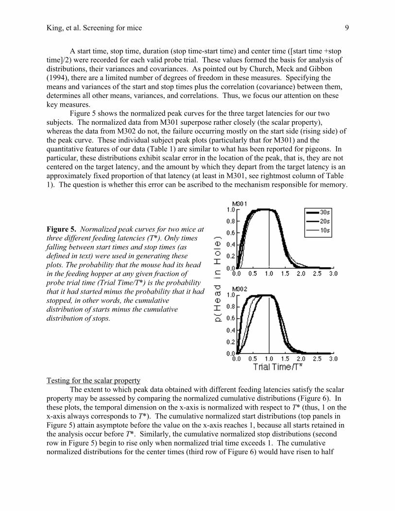
Figure 5 shows the normalized peak curves for the three target latencies for our twosubjects. The normalized data from M301 superpose rather closely (the scalar property),whereas the data from M302 do not, the failure occurring mostly on the start side (rising side) ofthe peak curve. These individual subject peak plots (particularly that for M301) and thequantitative features of our data (Table 1) are similar to what has been reported for pigeons. Inparticular, these distributions exhibit scalar error in the location of the peak, that is, they are notcentered on the target latency, and the amount by which they depart from the target latency is anapproximately fixed proportion of that latency (at least in M301, see rightmost column of Table1). The question is whether this error can be ascribed to the mechanism responsible for memory.

Figure 5. Normalized peak curves for two mice atthree different feeding latencies (T*). Only timesfalling between start times and stop times (asdefined in text) were used in generating theseplots. The probability that the mouse had its headin the feeding hopper at any given fraction ofprobe trial time (Trial Time/T*) is the probabilitythat it had started minus the probability that it hadstopped, in other words, the cumulativedistribution of starts minus the cumulativedistribution of stops.

Testing for the scalar propertyThe extent to which peak data obtained with different feeding latencies satisfy the scalar

property may be assessed by comparing the normalized cumulative distributions (Figure 6). Inthese plots, the temporal dimension on the x-axis is normalized with respect to T* (thus, 1 on thex-axis always corresponds to T*). The cumulative normalized start distributions (top panels inFigure 5) attain asymptote before the value on the x-axis reaches 1, because all starts retained inthe analysis occur before T*. Similarly, the cumulative normalized stop distributions (secondrow in Figure 5) begin to rise only when normalized trial time exceeds 1. The cumulativenormalized distributions for the center times (third row of Figure 6) would have risen to half


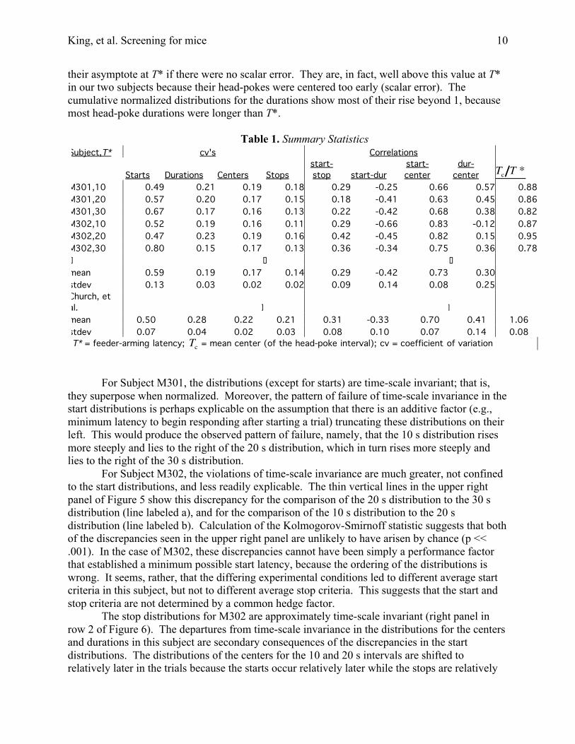
their asymptote at T* if there were no scalar error. They are, in fact, well above this value at T*in our two subjects because their head-pokes were centered too early (scalar error). Thecumulative normalized distributions for the durations show most of their rise beyond 1, becausemost head-poke durations were longer than T*.

Table 1. Summary StatisticsSubject,T* cv's Correlations

Starts Durations Centers Stopsstart-stop start-dur

start-center

dur-center

†

Tc T *M301,10 0.49 0.21 0.19 0.18 0.29 -0.25 0.66 0.57 0.88M301,20 0.57 0.20 0.17 0.15 0.18 -0.41 0.63 0.45 0.86M301,30 0.67 0.17 0.16 0.13 0.22 -0.42 0.68 0.38 0.82M302,10 0.52 0.19 0.16 0.11 0.29 -0.66 0.83 -0.12 0.87M302,20 0.47 0.23 0.19 0.16 0.42 -0.45 0.82 0.15 0.95M302,30 0.80 0.15 0.17 0.13 0.36 -0.34 0.75 0.36 0.78! ! !mean 0.59 0.19 0.17 0.14 0.29 -0.42 0.73 0.30stdev 0.13 0.03 0.02 0.02 0.09 0.14 0.08 0.25Church, etal. ! !mean 0.50 0.28 0.22 0.21 0.31 -0.33 0.70 0.41 1.06stdev 0.07 0.04 0.02 0.03 0.08 0.10 0.07 0.14 0.08T* = feeder-arming latency;

†

Tc = mean center (of the head-poke interval); cv = coefficient of variation

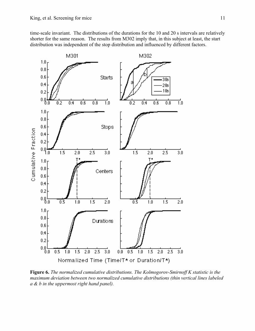
For Subject M301, the distributions (except for starts) are time-scale invariant; that is,they superpose when normalized. Moreover, the pattern of failure of time-scale invariance in thestart distributions is perhaps explicable on the assumption that there is an additive factor (e.g.,minimum latency to begin responding after starting a trial) truncating these distributions on theirleft. This would produce the observed pattern of failure, namely, that the 10 s distribution risesmore steeply and lies to the right of the 20 s distribution, which in turn rises more steeply andlies to the right of the 30 s distribution.

For Subject M302, the violations of time-scale invariance are much greater, not confinedto the start distributions, and less readily explicable. The thin vertical lines in the upper rightpanel of Figure 5 show this discrepancy for the comparison of the 20 s distribution to the 30 sdistribution (line labeled a), and for the comparison of the 10 s distribution to the 20 sdistribution (line labeled b). Calculation of the Kolmogorov-Smirnoff statistic suggests that bothof the discrepancies seen in the upper right panel are unlikely to have arisen by chance (p <<.001). In the case of M302, these discrepancies cannot have been simply a performance factorthat established a minimum possible start latency, because the ordering of the distributions iswrong. It seems, rather, that the differing experimental conditions led to different average startcriteria in this subject, but not to different average stop criteria. This suggests that the start andstop criteria are not determined by a common hedge factor.

The stop distributions for M302 are approximately time-scale invariant (right panel inrow 2 of Figure 6). The departures from time-scale invariance in the distributions for the centersand durations in this subject are secondary consequences of the discrepancies in the startdistributions. The distributions of the centers for the 10 and 20 s intervals are shifted torelatively later in the trials because the starts occur relatively later while the stops are relatively


time-scale invariant. The distributions of the durations for the 10 and 20 s intervals are relativelyshorter for the same reason. The results from M302 imply that, in this subject at least, the startdistribution was independent of the stop distribution and influenced by different factors.

Figure 6. The normalized cumulative distributions. The Kolmogorov-Smirnoff K statistic is themaximum deviation between two normalized cumulative distributions (thin vertical lines labeleda & b in the uppermost right hand panel).


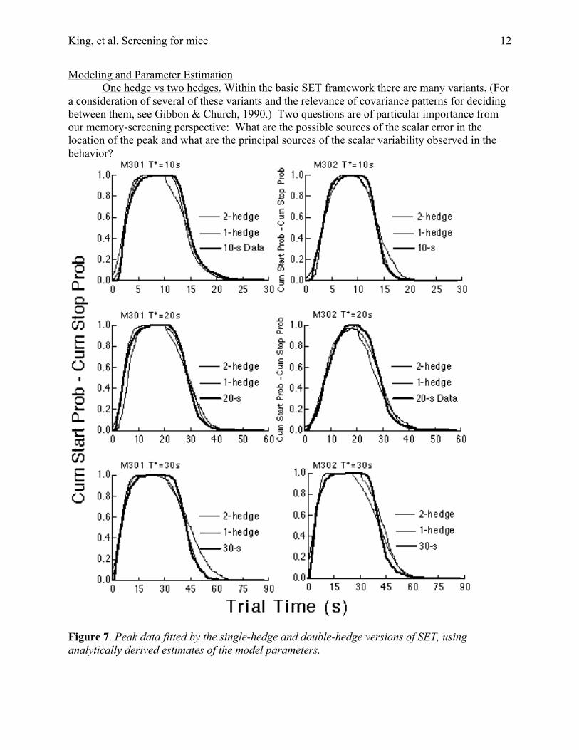
Modeling and Parameter EstimationOne hedge vs two hedges. Within the basic SET framework there are many variants. (For

a consideration of several of these variants and the relevance of covariance patterns for decidingbetween them, see Gibbon & Church, 1990.) Two questions are of particular importance fromour memory-screening perspective: What are the possible sources of the scalar error in thelocation of the peak and what are the principal sources of the scalar variability observed in thebehavior?

Figure 7. Peak data fitted by the single-hedge and double-hedge versions of SET, usinganalytically derived estimates of the model parameters.


If the SET model is to be used to estimate parameters of an underlying memory processfrom peak data, the first question to be addressed is how well the model describes the data fromindividual subjects. Given that few such analyses are available in the literature, we here examinethe SET model analytically and compare analytically derived parameter estimates with ourempirical data. Due to length constraints, we report here only important results of theseanalyses. For the analytic estimation of model parameters, see Appendix A.

Figure 7 shows the analytic fits of the 1-hedge and 2-hedge models to the data. These arethe fits obtained when the model parameters are estimated analytically, rather than by an iterativesearch for the permissible parameters that minimize the residual variance. The parameterestimation formula can, and sometimes did, yield negative variance estimates for the distributionof the stop threshold in the double-hedge model, because the variability in the stop distributionsis about the same as the covariance between starts and stops, which means that, according to thedouble-hedge model, memory variability is the only significant source of variability in stoptimes. In these cases, we used that assumption to model the data; that is, we took the variabilityin the underlying distribution of stop proportions to be negligible.

By some standards, the fits in Figure 7 are good; they account for a high percentage ofthe variance. However, the discrepancies between the data and the model’s predictions areclearly systematic. The observed distributions are more skewed than the distributions generatedby the models. One reason for the skew in the start distributions may be that they are truncatedon their left by the same factors that cause the failures to obtain scalar variability in startdistributions. Given these truncating factors, it is perhaps surprising that the model’s predictionsfit the data as well as they do. The reasons for the skew in the stop data are less obvious. Churchet al. (1991) investigated the sources of asymmetry in peak data at some length and identifiedseveral factors that skew the right side of the stop distribution.

The important point for our purpose is that the double-hedge model fits the data at leastas well as the single-hedge model. On the one hand, this is not surprising, because the double-hedge model has one more parameter. However, as Church, et al. (1994) point out, the patternsof variance and covariance also permit one to determine which is the better model, and thesefavor the double-hedge model in our data, just as they did in the data of Church, et al. (1994).The single-hedge model predicts that the cv for distributions of the centers of the head-pokeintervals should be less than the cv for both the start and the stop distributions, whereas, moreoften than not the cv of the stops is slightly less than the cv of the centers (Table 1). In otherwords, the variance in the centers is bigger than it ought to be relative to the variance in thestops. Also, the location of the center of a head-poke interval is not as strongly correlated withthe start of the interval as the single-hedge model says it should be. Church, et al. (1994) showedthat in the single-hedge model, this correlation should be equal to the ratio between the cv forcenters [cv(d)] and the cv for durations [cv(d)], whereas in both our data and theirs, it is less thanthis ratio, often much less (Figure 8)

In summary, the data give no reason to reject a double-hedge model; on the contrary, theyfavor it. Therefore, if starts and stops are independently hedged, the deviation of the center ofthe peak curve from the target latency is not an estimate of scalar memory error; in a two hedgeversion of SET no such estimate is possible. Our modeling with two independent hedge factorsemphasized this point by assuming that the scalar error in memory was zero. The expectation ofthe memory distribution was not a free parameter; it was set to the target time.


Figure 8. The correlations between durations andcenters (ordinate) plotted against the ratio of thecv’s. In the single hedge model, these points shouldcluster around the positive diagonal (solid line).

Memory variability. Which model one adopts is also important for estimating themagnitude of memory variability. In the single-hedge model, noise in the hedge factor has equaland opposite effects on the start and stop thresholds. A smaller than usual hedge factor leads to alate start and an equally early stop. Thus, variation in the centers of the head-poke intervals isdue entirely to memory variance. If, however, start and stop thresholds come from independentdistributions, then variance in the decision criteria does contribute to variance in the centers. Inthe double-hedge model, however, the start-stop covariance is proportional to the memoryvariance, because an unusually long sample from the memory distribution leads to a late start anda late stop. Thus, which aspect of the peak data estimates the memory variance depends on whichmodel one takes to be the right model.

In many published treatments of SET models, clock variance and memory variance aretreated as interchangeable (e.g., Church, et al., 1994) on the implicit or explicit assumption thatmemory variability is clock variability, because target latencies sampled from memory comefrom the population of experienced target latencies. Under this assumption, the variability in thememory samples and the variability in the experienced target latencies are identical results oftrial-to-trial variability in clock speed on feeding trials (Gibbon, 1977). Of course, it is possiblethat the variability in memory samples arises independently of variability in the input.

More importantly, if trial-to-trial variation in clock speed is the source of memoryvariability, then this clock variability should determine the observed variation in start and stoptimes in two ways, only one of which is reflected in the formulae in Table 2A (Appendix). On atrial when the clock runs slower than usual, the experienced feeding latency will be shorter thanusual, resulting in a shorter than usual record in memory. Similarly, on a trial when the clockruns faster than usual, the experienced feeding latency will be longer than usual. As alreadyexplained, this variation in experienced (subjective) feeding latencies will show up as variationin the remembered feeding latencies on probe trials.2 However, the variation in clock speed onthe probe trials themselves will also result in variation in the observed start and stop times.Whatever the start criterion is, it will take more time to reach it on trials when the clock runsslow and less time on trials when the clock runs fast.3

2 The resulting distribution of experienced feeding latencies in memory will be skewed toward longer latencies,because the experienced feeding latency tends to zero as clock speed tends to zero and it tends to infinity as clockspeed tends to infinity. The difference between a finite expectation and zero is equal to the expectation (hence,finite) while the difference between a finite expectation and infinity is itself infinite. However, the skew is smallwhen the coefficient of variation in clock speed is of the order seen in our data (0.2).3 This effect also yields a skew towards longer times for the same reasons: observed start times tend toward infinityas clock speed tends toward zero.


To address this issue, we developed a computer program (Appendix B) capable ofsimulating a variety of SET models, including those where clock variance and memory varianceare treated as separate sources of variability. Numerical simulation is necessary because whenboth memory variance and clock variance are treated as independent Gaussian variables,expressions involving the ratio between these variables are analytically intractable (they haveundefined variances).

In running our first simulation, we set the parameters of the model so as to duplicate theassumptions made by Church, et al. (1994) in deriving the formulae relating observedexpectations and variances to the expectations and variances in SET variables: They implicitlyassumed no variation in clock speed on probe trials, so we set this variation to zero in oursimulation. We set the expectation of the memory distribution to T* (the target time), and we setthe expectations and standard deviations of the distributions for the start and stop thresholdproportions (L and U) to the values we obtained analytically. We then varied the coefficient ofvariation for the distribution of

†

ˆ m (that is, memory variability).In the second simulation, we explored the effect of positing no memory variance, only

clock-speed variance. We set memory variability to zero and varied the clock speed. In the thirdsimulation, we allowed both memory variability and and variability in clock speed. The first twosimulations are the limiting cases of the third simulation. That is, in the first simulation, there isno variation in clock speed, only in memory samples; in the second simulation, there is novariation in memory samples, only in clock speed; in the third simulation, there is variation inboth clock speed and memory samples, as there would have to be in any model that positedvariation in clock speed as the source of variation in memory samples.

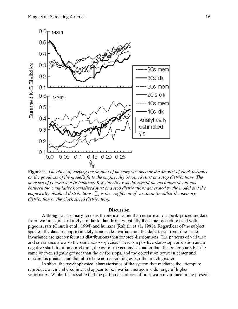
Figure 9 shows the results from the limiting cases (Simulations 1 and 2). A model inwhich clock speed varied but memory samples did not (dashed curves in Figure 8) tended to dobetter than a model in which memory samples varied but clock speed did not (solid curves inFigure 8). However, for most data sets, the goodness of the model's fit did not depend stronglyon the values of these gammas. In particular, the fits obtained with gammas of zero were noworse and sometimes better than the fits obtained with the analytically estimated values ofgamma.

The simulation with both memory variation and clock variation did not change thispicture: The best fit when both sources of covariation were present was only marginally betterthan the best fit in the limiting case where only clock speed was allowed to vary.

The most important conclusion that emerges from these simulations is that there are twopotential sources of the modest covariation between starts and stops seen in our data and in thedata of others (Church, et al., 1994; Gibbon & Church, 1990; Cheng & Westwood, 1993) (Chenget al., 1993) --trial-to-trial variation in clock speed and trial to trial variation in the target valuesampled from memory. Variation in clock speed may or may not be the source of the variation inmemory samples. Whether it is or not, it would seem that in these data one cannot separatelyestimate the two contributions—memory variance and clock variance.


Figure 9. The effect of varying the amount of memory variance or the amount of clock varianceon the goodness of the model's fit to the empirically obtained start and stop distributions. Themeasure of goodness of fit (summed K-S statistic) was the sum of the maximum deviationsbetween the cumulative normalized start and stop distributions generated by the model and theempirically obtained distributions.

†

ˆ g m is the coefficient of variation (in either the memorydistribution or the clock speed distribution).

DiscussionAlthough our primary focus is theoretical rather than empirical, our peak-procedure data

from two mice are strikingly similar to data from essentially the same procedure used withpigeons, rats (Church et al., 1994) and humans (Rakitin et al., 1998). Regardless of the subjectspecies, the data are approximately time-scale invariant and the departures from time-scaleinvariance are greater for start distributions than for stop distributions. The patterns of varianceand covariance are also the same across species: There is a positive start-stop correlation and anegative start-duration correlation, the cv for the centers is smaller than the cv for starts but thesame or even slightly greater than the cv for stops, and the correlation between center andduration is greater than the ratio of the corresponding cv’s, often much greater.

In short, the psychophysical characteristics of the system that mediates the attempt toreproduce a remembered interval appear to be invariant across a wide range of highervertebrates. While it is possible that the particular failures of time-scale invariance in the present


data are the result of behavioral tendencies particular to the mouse, we believe that a geneticdissection of this system in the mouse would have broadly applicable results.

The human data differ quantitatively from the rat, pigeon and our mouse data in tworespects: The peaks are much sharper and narrower, and the start-stop correlations are higher.The ratio of the width of the peak at half-maximum (mean stop minus mean start) to its modewas 1.1-1.6 in our two mice and 1.2 +/-0.08 in Church, et al.’s (1994) rats, whereas it was 0.34 –0.4 in the human data (see Table 2 on p. 22 of Rakitin et al., 1998). In rats and pigeons, and inour two mice, the start-stop correlations are roughly 0.3 +/-0.09, whereas in humans they areroughly 0.9 +/- 0.1 (see Figure 6 on p. 24 of Rakitin et al., 1998).

We have used our data to investigate the question whether peak data alone permit one toestimate two quantitative properties of the memory mechanism: The trial-to-trial variability in asample from memory, and the scalar error, that is the proportion by which the mean rememberedduration differs from the mean of the originally experienced durations. We conclude that thatpeak data alone do not permit one to estimate these memory parameters.

Whether one can estimate the scalar error from peak data hinges on whether there are orare not separate hedge factors for the start and stop criteria. If there is a single hedge factor, thenthe start and stop criteria on any trial are equidistant from the target sampled from memory, andsystematic deviation from the target time implies systematic error in the memory samples.(Cheng, 1992) found that when he penalized pigeons for starting sooner than half way to thefeeding (target) time, the pigeons started later and stopped sooner. That is, both the start criterionand the stop criterion moved closer to the target time. This counterintuitive result suggests thatthere is only one hedge factor.

However, data from our two mice, like comparable data from pigeons (Cheng &Westwood, 1993; Gibbon & Church, 1992), rats (Church et al., 1994) and humans (Rakitin et al.,1998), are more consistent with a two-hedge model than with a single-hedge model. In thesingle-hedge model, variance in the hedge factor contributes to variance in the starting andstopping times, but not to variance in the center because a small hedge produces a late start andan early stop, with mutually annulling effects on the center. Thus, only variance in the memorysample causes variance in the center. This source also contributes effects of equal magnitude tothe start and stop times. Thus, the variance of the center should be relatively less than both of thelatter variances. In fact, however, the cv for the center is consistently as large or larger than thecv for the stop–in our data and in others’ (Cheng & Westwood, 1993; Church et al., 1994;Gibbon & Church, 1992).

Second, in the single-hedge model, variance in the memory sample is the sole source ofthe variance of the center but one of two sources for the variance of the duration (the other beingvariance in the hedge factor). If memory were the sole source for both center and durationvariance, then the cv’s for the center and the duration would be equal and the correlationbetween the two variables would be perfect; the duration of a head poke would vary from trial totrial in proportion as the centers were late or early. However, to the extent that variance in thehedge factor contributes to variance in the duration, the cv for the duration should be greater thanthe cv for the center, and the correlation between the two variables should be correspondinglyless. Thus, the estimate for the correlation should on average equal the ratio of the two cvestimates. In fact, however, the estimated correlation is reliably less than this ratio (Figure 8), aspredicted by a two-hedge model.

Finally, it is clear in our data and in that of others that various experimental factors canaffect the start criterion either more or less than the stop criterion, which would not be possible if


there were only one hedge factor common to the two criteria. In the data presented here forM302, changing the target latency had non-scalar effects on the start criterion but scalar effectson the stop criterion. Church, et al. (1994, Figure 3. p. 138) found that the duration of peak trialsaffected the start criterion more than the stop criterion, whereas the stop criterion was affectedmore than the start criterion by whether the trial preceding the peak trial had been a feeding trialor another peak trial (a trial with no feeding—see their Figure 5, p. 139).

We conclude that peak data alone cannot distinguish variation in the degree ofasymmetry between start and stop criteria from variation in systematic memory error when thestart and stop criteria generally bracket the target time, as they do in our data (Figure 3). Wenote, however, that variation in the hedge factor or factors cannot shift the median of the startdistribution beyond the target time nor the median of the stop distribution before the target time,whereas variation in systematic memory error can shift either distribution arbitrarily far in eitherdirection. In the human timing literature, taking Parkinson’s patients off their L-DOPA can shifteither the start or the stop distributions so as to place their medians close to or even slightly tothe wrong side of the target value (Malapani et al., 1998), so effects of this magnitude couldreasonably be looked for in genetic screening. A shift of the median to the wrong side of thetarget value would be strong evidence of systematic memory error. Our raster plots (Figure 3)display the raw data from the peak procedure and related procedures in such a way that an effectof this kind would be immediately evident, without statistical treatment or modeling.

We also conclude that one cannot estimate the memory variance from peak data alone,again because of uncertainty about the correct version of the SET model. If, as appears likely, thestart and stop criteria are separately determined, then the covariance of the start and stopthresholds is the measure of memory variance—but only if the effects of the variation in clockspeed on the probe trials themselves (as opposed to on feeding trials) are assumed to benegligible. If, as has often been assumed, variation in clock speed is the source of variation inmemory samples, then it is implausible to assume that this variation is not also a factor on thepeak trials themselves. In any event, one needs a procedure that enables one to distinguishbetween covariation due to variation in the clock speed on peak trials and variation in thememory samples.

There are variants of the peak procedure that produce multiple possible targets on a singletrial (Cheng et al., 1993; Fetterman & Killeen, 1995; Mattell, King, & Meck, 2001). In general,they place responses controlled by different target latencies in competition, so that one responseis appropriate during one part of the peak trial whereas another response becomes appropriateduring another part of the same trial. These are likely to be useful in two respects: They shouldallow us to move start and stop criteria around independently (assuming that they can in fact shiftindependently), and they allow one to deconfound memory variance and clock variance (Chenget al., 1993). Thus, we think that using variants of the peak procedure to screen for abnormalitiesin the quantitative properties of memory merits continued investigation.

ReferencesAntoch, M. P., Song, E. J., Chang, A. M., Vitaterna, M. H., Zhao, Y., Wilsbacher, L. D.,

Sangoram, A. M., King, D. P., Pinto, L. H., & Takahashi, J. S. (1997). Functional identificationof the mouse circadian Clock gene by transgenic BAC rescue. Cell, 89(4), 655-667.

Aronson, L., Balsam, P. D., & Gibbon, J. (1993). Temporal comparator rules andresponding in multiple schedules. Animal Learning and Behavior, 21(4), 293-302.


Brunner, D., Fairhurst, S., Stolovitzky, G., & Gibbon, J. (1997). Mnemonics forvariability: Remembering food delay. Journal of Experimental Psychology: Animal BehaviorProcesses, 23(1), 68-83.

Catania, A. C., & Reynolds, G. S. (1968). A quantitative analysis of the respondingmaintained by interval schedules of reinforcement. Journal of the Experirmantal Analysis ofBehavior, 11, 327–383.

Cheng, K. (1992). The form of timing distributions in pigeons under penalties forresponding early. Animal Learning and Behavior, 20(2), 112-120.

Cheng, K., & Westwood, R. (1993). analysis of single trials in pigeon's timingperformance. Journal of Experimental Psychology: Animal Behavior Processes, 19, 56-67.

Cheng, K., Westwood, R., & Crystal, J. D. (1993). Memory variance in the peakprocedure of timing in pigeons. Journal of Experimental Psychology: Animal BehaviorProcesses, 19, 68-76.

Church, R. M., & Meck, W. H. (1988). Biological basis of the remembered time ofreinforcement. In M. L. Commons & R. M. church & J. R. Stellar & A. R. Wagner (Eds.),Quantitative analyses of beahvior: Biological determinants of reinforcement (Vol. 7, pp. 103-119). Hillsdale, NJ: Erlbaum.

Church, R. M., Meck, W. H., & Gibbon, J. (1994). Application of scalar timing theory toindividual trials. Journal of Experimental Psychology: Animal Behavior Processes, 20(2), 135-155.

Church, R. M., Miller, K. D., Meck, W. H., & Gibbon, J. (1991). Symmetrical andasymmetrical sources of variance in temporal generalization. Animal Learning and Behavior, 19,207-214.

Dunlap, J. C. (1993). Genetic analysis of circadian clocks. Annual Review of Physiology,55, 683-728.

Fantino, E., & Goldshmidt, J. N. (2000). Differences, not ratios, control choice in anexperimental analogue to foraging. Psychological Science, 11(3), 229-233.

Fetterman, J. G., & Killeen, P. R. (1995). Categorical scaling of time: Implications forclock-counter models. Journal of Experimental Psychology: Animal Behavior Processes, 21, 43-63.

Gallistel, C. R. (1990). The organization of learning. Cambridge, MA: BradfordBooks/MIT Press.

Gallistel, C. R. (1999). Can a decay process explain the timing of conditioned responses?Journal of the Experimental Analysis of Behavior, 71, 264-271.

Gallistel, C. R., & Gibbon, J. (2000). Time, rate and conditioning. Psychological Review,107, 289-344.

Gibbon, J. (1977). Scalar expectancy theory and Weber's Law in animal timing.Psychological Review, 84, 279-335.

Gibbon, J. (1991). Origins of scalar timing. Animal Learning and Behavior, 22, 3-38.Gibbon, J. (1992). Ubiquity of scalar timing with a Poisson clock. Journal of

Mathematical Psychology, 36, 283-293.Gibbon, J., & Church, R. M. (1981). Time left: linear versus logarithmic subjective time.

Journal of Experimental Psychology: Animal Behavior Processes, 7(2), 87-107.Gibbon, J., & Church, R. M. (1992). Comparison of variance and covariance patterns in

parallel and serial theories of timing. Journal of the Experimental Analysis of Behavior, 57, 393-406.


Gibbon, J., Church, R. M., & Meck, W. H. (1984). Scalar timing in memory. In J. Gibbon& L. Allan (Eds.), Timing and time perception (Vol. 423, pp. 52-77). New York: New YorkAcademy of Sciences.

Gibbon, J., & Fairhurst, S. (1994). Ratio versus difference comparators in choice. Journalof the Experimental Analysis of Behavior, 62, 409-434.

Gibbon, J., Malapani, C., Dale, C. L., & Gallistel, C. R. (1997). Toward a neurobiologyof temporal cognition: Advances and challenges. Current Opinion in Neurobiology, 7(2), 170-184.

Leak, T. M., & Gibbon, J. (1995). Simultaneous timing of multiple intervals:Implications for the scalar property. Journal of Experimental Psychology: Animal BehaviorProcesses, 21(1), 3-19.

Malapani, C., Rakitin, B. C., Levy, R., Meck, W. H., Deweer, B., Dubois, B., & Gibbon,J. (1998). Coupled temporal memories in Parkinson's disease: a depamine-related dysfunction.Journal of Cognitive Neuroscience, 10, 316-331.

Mattell, M. S., King, G. R., & Meck, W. H. (2001). Differential modulation of peak timesin the tri-peak procedure by the chronic administration of intermittent or continuous cocaine. MS(pp. 29).

Meck, W. H., & Church, R. M. (1984). Simultaneous temporal processing. . Journal ofExperimental Psychology: Animal Behavior Processes., 10, 1-29.

Meck, W. H., & Church, R. M. (1987). Cholinergic modulation of the content oftemporal memory. Behavioral Neuroscience, 101, 457-464.

Rakitin, B. C., Gibbon, J., Penney, T. B., Malapani, C., Hinton, S. C., & Meck, W. H.(1998). Scalar expectancy theory and peak-interval timing in humans. Journal of ExperimentalPsychology: Animal Behavior Processes, 24(1), 15-33.

Rescorla, R. A. (1998). Instrumental learning: Nature and persistence. In M. Sabourin &F. I. M. Craik & M. Roberts (Eds.), Proceeding os the XXVI International Congress ofPsychology: Vol. 2. Advances in psychological science: Biological and cognitive aspects (Vol. 2,pp. 239-258). London: Psychology Press.

Roberts, S. (1981). Isolation of an internal clock. Journal of Experimental Psychology:Animal Behavior Processes, 7, 242-268.

Roberts, S., & Church, R. M. (1978). Control of an internal clock. Journal ofExperimental Psychology: Animal Behavior Processes, 4, 318-337.

Roberts, W. A., & Boisvert, M. J. (1998). Using the peak procedure to measure timingand counting processes in pigeons. Journal of Experimental Psychology: Animal BehaviorProcesses, 24(4), 416-430.

Tang, Y.-P., Shimizu, E., Dube, G. R., Rampon, C., Kerchner, G. A., Zhuo, M., Liu, G.,& Tsien, J. Z. (1999). Genetic enhancement of learning and memory in mice. Nature, 401, 63-69.

Vicens, P., Bernal, M. C., Carrasco, M. C., & Redolat, R. (1999). Previous training in thewater maze: Differential effects in NMRI and C57BL mice. Physiology & Behavior, 67(2). 197-203.

Wilkie, D. M., Willson, R. J., & Carr, J. A. R. (1999). Errors made by animals in memoryparadigms are not always due to failure of memory. Neuroscience & Biobehavioral Reviews,

23(3). 451-455.

Acknowledgments


This research was supported by NIMH Grant 1R21MH63866 to CRG. The assistance of MarioWalls and Yair Ghitza is gratefully acknowledged

Appendix A: Formulae and DerivationsThe formulae used to estimate model parameters from the data are given in Table 1A.

They derive from formulae in Church, Meck and Gibbon (1994), which go back in turn toderivations in the Appendix to Gibbon & Church (1992). We briefly recapitulate essential steps,because it is difficult to pull them together.

The memory for the target latency is sampled once on each trial, yielding a quantitydenoted ˆ m . Either one or two variable hedge factors are also sampled. The observed variability

in starts and stops is determined by trial-to-trial variability in ˆ m and in the hedge factors.Although Church, et al. (1994) refer to ˆ s m

2 , the variance of ˆ m , sometimes as memoryvariance and sometimes as clock variance, their formulae implicitly assume that trial-to-trial variation in clock speed on probe trials makes a negligible contribution to theobserved variation in starts and stops. The observed variance in start times, s t l

2 , is due to the

variance, ˆ s lm2 , of the start criteria, ˆ l ˆ m which is equal to the variance in the products of ˆ l and

ˆ m . From the rule for the variance of products, we have:

s t l

2 = ˆ s l2 ˆ s m

2 + ˆ L 2 ˆ s m2 + ˆ M 2 ˆ s l

2 .(1)

(Capital letters denote expectations.) The right hand side of Equation (1) may be rewritten in theform, ˆ s l

2( ˆ s m2 + ˆ M 2 ) + ˆ L 2 ˆ s m

2 . The same reasoning leads to the formula relating modelparameters to the observed variance in stops:s t u

2 = ˆ s u2 ˆ s m

2 + ˆ U 2 ˆ s m2 + ˆ M 2 ˆ s u

2 = ˆ s m2 ( ˆ s u

2 + ˆ U 2 ) + ˆ M 2 ˆ s u2 . (2)

In the single-hedge model, it is assumed that there is only one hedge factor, ˆ b , withˆ l = 1- ˆ b and ˆ u = 1+ ˆ b . Scalar error in the observed mean center, Tc , is then an estimate of the

scalar memory error,

†

Km , and the observed variance of the center points, sc2 , is an estimate of

the variance of the memory distribution (for derivations, see Gibbon & Church, 1992).

In the double-hedge model, the proportions ˆ l and ˆ u are drawn from differentdistributions. Then, the only source of covariance between start and stop times is the memorysample. This covariance, when divided by the product of the expectations of the start and stopproportions, gives an estimate of the memory variance. The derivation follows from the generalformula for covariance:2Cov(t l ,tu ) = 2Cov(ˆ l ˆ m , ˆ u ˆ m ) = Var(ˆ l ˆ m + ˆ u ˆ m ) - ( ˆ s lm

2 + ˆ s um2 ) .(3)

Because ˆ l and ˆ u are assumed to vary independently, their variation does not contribute to the

covariation in ˆ l ˆ m and ˆ u ˆ m , so we can replace ˆ l and ˆ u with their expectations, ˆ L and ˆ U , whichare constants. Examining one by one the two terms on the right hand side of Equation (3), wefind that:Var ( ˆ L ̂ m + ˆ U ˆ m ) = Var[ ˆ m ( ˆ L + ˆ U )] = ˆ s m

2 ( ˆ L + ˆ U )2 = ˆ s m2 ˆ L 2 + 2 ˆ L ˆ U + ˆ U 2( )

and


ˆ s Lm2 + ˆ s Um

2( ) = ˆ L 2 ˆ s m2 + ˆ U 2 ˆ s m

2 = ˆ s m2 ˆ L 2 + ˆ U 2( ) .

The squares of the expectations and the factor 2 cancel out, leaving Cov(t l ,tu ) = ˆ U ̂ L ˆ s m2 .

The peak curve (whether predicted or observed) is the cumulative start distribution minusthe cumulative stop distribution.

Table 1A. NotationVariable Symbol

Objective time

†

tSubjective time

†

ˆ t Target reward. time (arming latency)

†

T *

Observed time of reward

†

tr

Subjective time of reward

†

ˆ t rObserved start time

†

tl

Observed stop time

†

tu

Observed center

†

tu - tl( ) 2

†

tc

Memory scalar (whose expectation [ ˆ K m ] is commonly symbolized by K*)

†

ˆ k mA reward latency sampled from memory

†

ˆ m Clock speed on a given trial

†

ˆ s Delay in starting the clock on a given trial

†

ˆ d Start criterion (as a proportion of

†

ˆ m )

†

ˆ l Stop criterion (as a proportion of

†

ˆ m )

†

ˆ u Start hedge factor (1-

†

ˆ l )

†

ˆ b lStop hedge factor (1-

†

ˆ u )

†

ˆ b uConventions: An italicized small letter is the name of a variable; for example,

†

t = elapsedtime in a trial. A hat (e.g.

†

ˆ t ) indicates that it is a subjective variable (not directly measurable);thus

†

ˆ t = subjective elapsed time in a trial. Absence of a hat indicates that it is an objective(directly measurable) quantity. Many variables are assumed Gaussian random, in which case,the upper case version of the letter is the expectation of the distribution, a lower case sigmasubscripted by the letter (in text not italic form) is the standard deviation of the distribution,and a lower case gamma, similarly subscripted, is the coefficient of variation. An italicized ias a subscript indicate that a particular value, the ith value, of the random variable is beingreferred to. Thus,

†

ˆ m refers to reinforcement times sampled from memory.

†

ˆ M and

†

ˆ s m are the

expectation and standard deviation of the sampled distribution, and

†

ˆ m i is the sample on trial i.

Table 2A :Formulae for Estimating Model Parameters from Data

Model & Model Parameter Estimation Formula

Single Hedge Factorˆ M = expectation of target latency

distribution

Med(tc )


distributionˆ s

m

2 = variance of remembered target

latency distribution

sc2

ˆ B = expectation of the hedge factordistribution

Med(tu ) - Med(tl )2Med(tc)

ˆ s b2 = variance of the hedge factor

distribution = the variance of both thestart & stop proportions

s t l

2 + s t u

2 - 2 ˆ s m2 (1+ ˆ B 2 )

2 ˆ s m2 + ˆ M 2( )

, the average of the

estimates obtained from the distributions ofstart and stop times

Two Hedge Factorsˆ L = expectation of start proportions Med(tl ) T *

ˆ U = expectation of stop proportions Med(tu ) T *

ˆ s m

2 = variance of remembered feeding

latencies

Cov(t l ,tu )ˆ U ̂ L

ˆ s l2 = variance of start proportions s t l

2 - ˆ L 2 ˆ s m2

ˆ s m2 + T *2

ˆ s u2 = variance of stop proportions s t u

2 - ˆ U 2 ˆ s m2

ˆ s m2 + T *2

Notation for observed or known quantitiesT * = target latency (programmed feeding time)t l = start timetu = stop time

tc = center point (middle) of a head-poke interval = t l + tu

2l = t l tcu = tu tc

sc2 = variance of center points


Appendix B: SimulationThe SET framework implemented in the simulation is the one portrayed in Figure 1.

Specifying different parameter values and different memory-sampling options creates variants ofthe basic SET model. The program runs a user-specified number of trials, containing a user-specified proportion of probe trials, to generate distributions of starts, stops, centers and spreads.The program compares the cumulative normalized start and stop distributions it generates to thecumulative normalized distributions obtained from individual subjects. The degree of mismatchbetween the model output and the obtained distributions is measured by the sum of the K-Sstatistics for the start and stop distributions. The program can vary user-specified modelparameters over a range of user-specified steps in a search for the parameter combination thatminimizes this measure of the discrepancy between model output and data. The user can thenexamine the variance and covariance patterns generated by the model using the best-fittingparameter values to determine the extent to which those patterns correspond to the patterns in thedata.4 The program for simulating SET modesl is available upon request from APK.

The simulation allows one to specify the following parameters and memory-samplingoptions:

• The expectation (

†

ˆ D ) and standard deviation (

†

sd ) of the delay (

†

ˆ d ) in starting the timer.• The standard deviation (

†

ˆ s s of the clock speed (

†

ˆ s ), which is the slope of the function relatingobjective duration to subjective duration. The expectation of this slope distribution is 1,because, in this framework, variation in its expectation has no observable effect.

• T*, the feeding latency• The expectation (

†

ˆ K m ) of the memory scalar (

†

ˆ k m ), which is the multiplicative factor relatingan experienced feeding latency (

†

ˆ t r ) to the record of that same latency when retrieved frommemory. In the figure, this scalar distortion is shown on the input side of memory, butconceptually it could be either on the input or the output. It allows for a calibration error inmemory, a systematic discrepancy between originally experienced durations andremembered durations. A calibration error exists if the expectation is some value otherthan 1.

• The standard deviation of the memory scalar (

†

ˆ k m ). The noise in this scalar can create apopulation of different remembered feeding latencies in the absence of variation in T*and/or clock speed.

• The memory sampling process on probe trials: The options are:i) Pick a random value from the population in memory resulting from trials where food was

obtained (feeding trials)ii) Take the mean or median of the population in memoryiii) Take the minimum value in memoryiv) Take a user-specified fixed value (e.g., T*) that is independent of the values

experienced on feeding trials•

†

ˆ g m = the coefficient of variation of the distribution of memory values (target values) on probetrials. If the memory sampling process yields a fixed or little varying value (as happens ifoptions ii - iv above are specified), then this allows for the introduction of variation in the

4 The program may be downloaded from the following web site:


samples actually used as the targets, variation that is independent of variation in the inputsto memory.

•

†

ˆ L = the expectation of the start proportion•

†

ˆ s l = the standard deviation of the start proportion•

†

ˆ U = the expectation of the stop proportion•

†

ˆ s u = the standard deviation of the stop proportion

Footnotes

1 The error may arise either in the write-to-memory operation or in the read-from-memory operation or as a combined result of quantitative errors in these two elementaryoperations.

Documents

Screening for Mice that Remember Incorrectlyruccs.rutgers.edu/images/personal-charles-r-gallistel/publications... · Screening for Mice that Remember Incorrectly Adam Philip King1