Atmos. Chem. Phys., 17, 9417–9433, 2017https://doi.org/10.5194/acp-17-9417-2017© Author(s) 2017. This work is distributed underthe Creative Commons Attribution 3.0 License.

Sea ice as a source of sea salt aerosol to Greenland ice cores:a model-based studyRachael H. Rhodes1, Xin Yang2, Eric W. Wolff1, Joseph R. McConnell3, and Markus M. Frey2

1Department of Earth Sciences, University of Cambridge, Cambridge, CB2 3EQ, UK2British Antarctic Survey, Natural Environment Research Council, Cambridge, CB3 0ET, UK3Division of Hydrologic Sciences, Desert Research Institute, Reno, NV 89512, USA

Correspondence to: Rachael H. Rhodes (rhr34@cam.ac.uk)

Received: 2 February 2017 – Discussion started: 2 March 2017Revised: 21 June 2017 – Accepted: 4 July 2017 – Published: 7 August 2017

Abstract. Growing evidence suggests that the sea ice sur-face is an important source of sea salt aerosol and this hassignificant implications for polar climate and atmosphericchemistry. It also suggests the potential to use ice core seasalt records as proxies for past sea ice extent. To explore thispossibility in the Arctic region, we use a chemical transportmodel to track the emission, transport, and deposition of seasalt from both the open ocean and the sea ice, allowing usto assess the relative importance of each. Our results confirmthe importance of sea ice sea salt (SISS) to the winter Arc-tic aerosol burden. For the first time, we explicitly simulatethe sea salt concentrations of Greenland snow, achieving val-ues within a factor of two of Greenland ice core records. Oursimulations suggest that SISS contributes to the winter max-ima in sea salt characteristic of ice cores across Greenland.However, a north–south gradient in the contribution of SISSrelative to open-ocean sea salt (OOSS) exists across Green-land, with 50 % of winter sea salt being SISS at northern sitessuch as NEEM (77◦ N), while only 10 % of winter sea saltis SISS at southern locations such as ACT10C (66◦ N). Ourmodel shows some skill at reproducing the inter-annual vari-ability in sea salt concentrations for 1991–1999, particularlyat Summit where up to 62 % of the variability is explained.Future work will involve constraining what is driving thisinter-annual variability and operating the model under differ-ent palaeoclimatic conditions.

1 Introduction

Salty blowing snow lofted from the surface of sea ice maybe an important source of sea salt aerosol to the polar at-mosphere (Yang et al., 2008), with significant implicationsfor climate and atmospheric chemistry. Sea salt aerosol actas cloud-condensation nuclei (O’Dowd et al., 1997) and icenucleating particles (DeMott et al., 2016), impacting radia-tive forcing (Murphy et al., 1998), as well as providing sur-faces for heterogeneous chemical reactions that impact thelevels of key atmospheric trace gases, such as ozone (Knip-ping and Dabdub, 2003; Yang et al., 2010). For palaeoclimat-ogists, this new source of sea salt provides a mechanism thatlinks the sea salt concentrations recorded in ice cores to seaice extent, potentially validating the use of sea salt as a seaice proxy (Abram et al., 2013).

Although early interpretations of ice core records assumedthat sea salt was only sourced from bubble bursting at theocean surface (e.g. Petit et al., 1999), two simple observa-tions presented a paradoxical view: (1) seasonal sea salt max-ima in most ice cores occur in winter not summer, and (2) seasalt concentrations are highest in glacial periods not inter-glacial periods. Given that sea ice extent is larger in winterrelative to summer, and in glacials relative to interglacials, wewould expect lower sea salt in winter and glacials if the openocean was the only source of sea salt, due to the longer trans-port time between the open ocean and the ice sheet. Clearlythat is not the case, and so, barring an unrealistic change inmeteorological conditions, another source of sea salt mustexist in winter (Wagenbach et al., 1998). Further evidencefor an additional source comes from Antarctic snow chem-

Published by Copernicus Publications on behalf of the European Geosciences Union.

9418 R. H. Rhodes et al.: Sea ice as a source of sea salt aerosol to Greenland ice cores: a model-based study

istry that reveals reduced SO2−4 : Na+ values, relative to sea

water, during winter months (Jourdain et al., 2008; Wagen-bach et al., 1998). Unlike NaCl, which contains reactive Cl−

(Keene et al., 1990; Röthlisberger et al., 2003), Na2SO4 isnot fractionated in the atmosphere or following deposition,confirming that a source of fractionated sea salt exists in win-ter.

Sea ice fits the bill – its areal extent is greatest in winter,and its surface is covered by salty snow and frost flowers,which contain reduced SO2−

4 : Na+ sea salt (Domine et al.,2004; Yang et al., 2008). Fractionation of SO2−

4 : Na+ rela-tive to sea water results from the precipitation of mirabilitesalt (Na2SO4

q10H2O) from brine in the channels that dissectthe sea ice (Butler and Kennedy, 2015), and from sea wa-ter that floods or inundates slabs of sea ice (Massom et al.,2001). Frost flowers are now thought to make a relativelysmall contribution to the sea salt aerosol load sourced fromthe sea ice surface because of their high mechanical strength(Obbard et al., 2009), subsequent lack of observed aerosolproduction (Yang et al., 2017), even under high wind speeds(Roscoe et al., 2011), and limited spatial and temporal range(Kaleschke et al., 2004; Perovich and Richter-Menge, 1994).

The model of Yang et al. (2008) proposes that the principalsource of sea salt from the sea ice surface is the entrainmentof salty snow particles by high winds during blowing snowevents, known to occur in the Antarctic (Mann et al., 2000;Nishimura and Nemoto, 2005) and Arctic (Savelyev et al.,2006). The air within the blowing snow layer is saturated forwater vapour, but the relative humidity reduces with height(Mann et al., 2000), allowing the water content of snow par-ticles to sublime, generating sea salt aerosol (Déry and Yau,2001).

The sea ice source of sea salt aerosol appears to be crit-ical for polar atmospheric chemistry. Domine et al. (2004)suggest that the salty snow on sea ice is an important sourceof Br− ions that contribute to the ozone depletion events ob-served over the sea ice in the spring. This idea is supported byevidence of air masses associated with ozone depletion orig-inating from the sea ice zone (Jones et al., 2009). Yang et al.(2010) used a modelling approach to demonstrate that blow-ing snow provided the additional sea salt aerosol required tosustain the high levels of BrO responsible for the destructionof ozone in the polar regions.

To explore the implications of this additional source of seasalt aerosol for sea ice proxy development, a chemical trans-port model can be used to represent emission, transport anddeposition of sea salt aerosol. Using this approach, Levine etal. (2014) found that sea-ice-sourced sea salt made a signifi-cant contribution to the winter sea salt aerosol budget at var-ious Antarctic locations, and that this improved the model–data match with aerosol observations. Recently, these resultshave been replicated (Legrand et al., 2016) and confirmedusing a different model (GEOS-Chem) with similar param-eterizations of sea salt emissions (Huang and Jaeglé, 2017).

Table 1. Parameters chosen for p-TOMCAT base simulation 1991–2006.

Parameter Value/setting used Reference

OOSS emissions OOSS emission by bub-ble bursting + SST de-pendence

Gong et al. (2003)+ Jaeglé et al.(2011)

SISS emissions SISS emission via blow-ing snow

Yang et al. (2008)

Snow salinity mean 0.6 psu (Arctic)Snow age 24 h (Arctic)Multi-year sea ice SISS emissions are re-

duced by 50 % relativeto first-year sea ice

Huang and Jaeglé (2017) also argue for the importance of theblowing snow sea salt source in the Arctic region.

Here we investigate sea salt in the Arctic region in greaterdepth, with a particular emphasis on how sea-ice-sourced seasalt may impact the sea salt budget of Greenland ice cores.Doing so should help us to decipher whether Greenland icecore sea salt records have any potential to record past sea icechanges in the Arctic.

2 Methods

In this study, our base simulation, run from 1991 to 2006, istuned (Table 1) to sea salt aerosol observations from acrossthe Arctic. The influence of various tuning parameters istested in sensitivity tests (Sect. 3). The performance of ourchemical transport model at simulating the concentration ofsea salt deposited in snow on the Greenland ice sheet is eval-uated by comparing simulations of monthly mean sea saltconcentrations in snowfall to values in Greenland ice cores(Sect. 4).

2.1 Arctic sea salt aerosol data

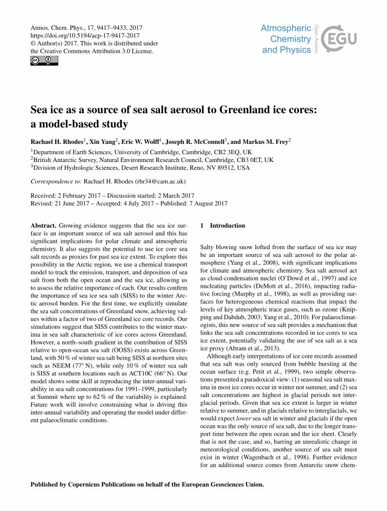
We use sea salt aerosol data from five Arctic locations as tar-gets for tuning our chemical transport model (Fig. 1). Thefive Arctic aerosol sites are Barrow in Alaska (Quinn et al.,2002), Alert in Canada (Barrie, 1995), Zeppelin Station onSvalbard, Villum Station in northern Greenland, and Sum-mit on the Greenland ice sheet (see the Supplement for de-tail on Summit aerosol data). For additional assessment ofthe model’s skill at representing sea salt aerosol in the atmo-sphere, we also compare model output to measurements fromfive low/mid-latitude aerosol sampling stations (Fig. S1 inthe Supplement) in the AEROCE-SEAREX network (Savoieet al., 2002). The age range of the aerosol data from eachsite is displayed in black on any figure where the data are in-cluded. Aerosol data are compared to model output for 0.1–5 µm dry particle radius (rdry).

Atmos. Chem. Phys., 17, 9417–9433, 2017 www.atmos-chem-phys.net/17/9417/2017/

R. H. Rhodes et al.: Sea ice as a source of sea salt aerosol to Greenland ice cores: a model-based study 9419

Figure 1. Map of the Arctic region showing locations of aerosolsampling stations (black circles) and ice cores (green circles) usedin this study. Contoured shading is mean February fractional sea icecoverage for 1991–1999, as prescribed in p-TOMCAT.

2.2 Greenland ice core sea salt records

Greenland ice core Na records (Fig. 1, Table 2) from 1991to 1999 are compared with simulations for the same time in-terval. The simulations include model output from the entirerdry range (0.1 to 10 µm).

All the ice cores were analysed using the continuousmelter system at the Desert Research Institute, Reno, USA(McConnell et al., 2002). Na was measured by high-resolution inductively coupled plasma mass spectrometry(HR-ICP-MS) with an estimated reproducibility of < 2 ppb(2σ ). The records are dated by annual layer counting ofmultiple chemical species that typically show different tim-ings of seasonal maxima – e.g. sea salt, mineral dust, andbiomass burning products (Sigl et al., 2013). All the cores,except Tunu13, have accumulation rates > 200 kg m−2 yr−1

(Table 2), providing monthly resolution records with age un-certainty of < 0.25 years. Uncertainty on dating at the sub-annual scale originates from the uncertainty in the absolutetiming of each seasonal marker and the assumption of a con-stant annual snow accumulation rate.

2.3 Chemical transport model

2.3.1 Model description

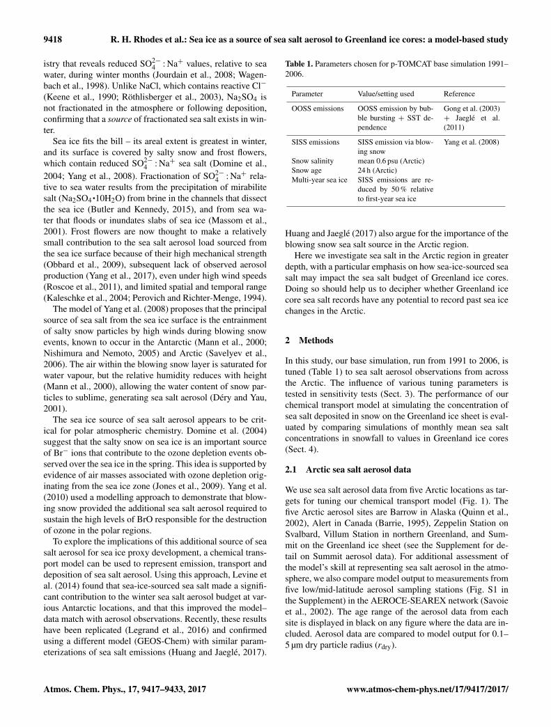
We use a simplified version of the Cambridge parallelizedTropospheric Offline Model of Chemistry and Transport (p-TOMCAT) to simulate the emission, transport and depositionof sea salt aerosol (Fig. 2), following the work of Levine et al.(2014). p-TOMCAT is a 3-D global model with a spatial res-

olution of 2.8◦× 2.8◦ across 31 vertical sigma-pressure lev-els. Here we only describe changes to the model parameteri-zation implemented since the study of Levine et al. (2014).

In this study, we drive p-TOMCAT with 6-hourly tem-perature, wind and humidity fields from the European Cen-tre for Medium-Range Weather Service Forecasts (ECMWF)ERA-Interim reanalysis data set (Dee et al., 2011) whereasLevine et al. (2014) used ECMWF operational data. The sig-nificant precipitation bias of p-TOMCAT (Giannakopouloset al., 2004) is remedied by applying a correction to forcethe simulated precipitation values towards Global Precipi-tation Climatology Project (GPCP) observations (Adler etal., 2003), following Legrand et al. (2016). The correctedprecipitation fields are used in wet deposition calculations(Sect. 2.3.3).

Sea salt aerosol particles are traced from emission to de-position in 21 size bins ranging from 0.1 to 10 µm rdry. Theambient radius (rwet) of each particle may change each timestep according to relative humidity and temperature. Particlessourced from the open-ocean and the sea ice surface, whichwe will refer to as open-ocean sea salt (OOSS) and sea icesea salt (SISS) respectively, are treated separately, giving atotal of 42 tracers. In p-TOMCAT, sea salt (SISS or OOSS)is assumed to be pure NaCl.

2.3.2 Sea salt emissions

Parameterization of OOSS emissions follows Gong (2003)and is based on the classic Monahan (1986) model of aerosolproduction via bubble bursting (Fig. 2). Gong et al.’s schemeis modified to account for a dependence of sea salt aerosolproduction on sea surface temperature (SST) (Eq. 4 of Jaegléet al., 2011).

Parameterization of SISS emissions follows Yang et al.(2008) (Eqs. 1–8) and this requires salinity and particle sizedistributions of snow particles entrained from the sea icesurface during blowing snow events to be defined (Fig. 2).We use new observations made during a wintertime cruiseof the RV Polarstern (June–August 2013) in the Wed-dell Sea, Antarctica. These measurements were conductedin the framework of the BLOWSEA project led by theBritish Antarctic Survey (https://doi.org/10.5285/c0261633-fd14-4d45-a58d-72998816c4cd; Frey, 2017). The salinitydistribution only includes measurements from the top 10 cmof the snow pack, as this snow is the most likely to be loftedup. Any individual salinity measurements > 10 psu are ex-cluded from the distribution. The mean salinity is 0.30 psu,which is 14-fold lower than that of the salinity distributionused by Levine et al. (2014) (4.25 psu) for snow on Antarc-tic sea ice. In our base simulation, this salinity distribution isdoubled for snow on Arctic sea ice (Table 1, Sect. 3.3.1). Theprobability density function that defines the size distributionof suspended particles in blowing snow events (Yang et al.,2008, their Eq. 6) has a snow particle radius of 70.3 µm andshape parameter (α) value of 2. p-TOMCAT does not simu-

www.atmos-chem-phys.net/17/9417/2017/ Atmos. Chem. Phys., 17, 9417–9433, 2017

9420 R. H. Rhodes et al.: Sea ice as a source of sea salt aerosol to Greenland ice cores: a model-based study

Table 2. Key characteristics of Greenland ice core records used.

Ice core LocationElevation Accumulation ratea Distance to coast Record end

Reference(m) (kg m−2 yr−1) (km) (year)

Tunu13 78◦ 2.09′ N, 33◦ 52.80′W 2105 112 300 2011 Maselli et al. (2017)NEEM-2011-S1b 77◦ 26.93′ N, 51◦ 03.37′W 2454 203 280 1997.5 Sigl et al. (2013)NEEM-2008-S3b 77◦ 26.93′ N, 51◦ 03.37′W 2454 203 280 2001NEEM-2010-20mb 77◦ 26.93′ N, 51◦ 03.37′W 2454 203 280 2008Summit2010 (a.k.a. Zoe2) 72◦ 36.0′ N, 38◦ 18.0′W 3258 222 530 2010 Maselli et al. (2017)D4 71◦ 24.0′ N, 43◦ 54.0′W 2730 414 320 2003 Banta et al. (2008)D5 68◦ 30.0′ N, 42◦ 54.0′W 2468 373 350 1998 Banta et al. (2008)Das2 67◦ 30.0′ N, 36◦ 06.0′W 2936 833 110 2003 Banta et al. (2008)Das1c 66◦ 00.0′ N, 44◦ 00.0′W 2497 600 200 2003 Banta et al. (2008)ACT10Cc 65◦ 59.93′ N, 42◦ 47.0′W 2299 809 200 2009.5ACT3c 66◦ 00.0′ N, 43◦ 36.0′W 2508 658 200 2005ACT2d 66◦ 00.0′ N, 45◦ 12.0′W 2419 372 240 2004 Banta et al. (2008)ACT11dd 66◦ 28.8′ N, 46◦ 18.6′W 2296 339 240 2011

a Water-equivalent accumulation rate. b Same grid square in p-TOMCAT. c Same grid square in p-TOMCAT. d Same grid square in p-TOMCAT

Figure 2. Schematic of processes parameterized by p-TOMCAT that influence sea salt concentrations in the atmosphere and ice cores.

late snow particles splitting into multiple individual sea saltaerosol (see Huang and Jaeglé, 2017).

The parameterization of SISS production by Yang et al.(2008) includes a parameter called snow age (t in Yang etal.’s Eq. 5), adopted from Box et al. (2004). A higher valueof snow age decreases SISS emissions, loosely representinghow sintered snow flakes are likely more difficult to mobilizethan fresh ones. Levine et al. (2014) found that the precipi-tation frequency and intensity within p-TOMCAT was notsuitable for defining a transient snow age so a constant valueof 5 days was used. When combined with our reduced snowsalinity, this high snow age, which reduces the amount ofblowing snow by almost a factor of 4 compared to a snowage of zero, resulted in extremely low SISS emissions. Sinceit is not clear that the parameterization of snow age has anyfirm basis for the very cold conditions encountered in theArctic, we used snow age as a crude tuning device, and (as

discussed in Sect. 3.3.3) adopted a value of 24 h for our basesimulation (Table 1).

Finally, the “gustiness factor” used by Levine et al. (2014)to increase the 6-hourly wind speeds used for sea salt aerosolemissions has been removed because it is specific to a dif-ferent chemical transport model (Gong et al., 2002). Wehave not replaced this value so peak sea salt emissions maybe underestimated due to the 6-hourly averaging of windspeeds. Sensitivity testing indicates that using a “gustinessfactor” decreases the correspondence between model resultsand aerosol data at Arctic sites (Fig. S4).

2.3.3 Sea salt deposition

The deposition of OOSS and SISS in p-TOMCAT followsthe parameterizations of Reader and MacFarlane (2003) (seealso Levine et al., 2014, Eqs. 1–9). Wet deposition via nucle-ation and collision are both parameterized by exponential de-

Atmos. Chem. Phys., 17, 9417–9433, 2017 www.atmos-chem-phys.net/17/9417/2017/

R. H. Rhodes et al.: Sea ice as a source of sea salt aerosol to Greenland ice cores: a model-based study 9421

cay. Collision scavenging is determined by the collision scav-enging parameter (αC, units: m2 kg−1) that varies with rwetand by the rate of precipitation occurring at the same atmo-spheric level and all levels above (PCL, units: kg m−2 s−1).Nucleation scavenging is dependent on the nucleation scav-enging parameter (αN, units of m2 kg−1) and the rate of pre-cipitation occurring only within the same atmospheric level(PNL, units: kg m−2 s−1). Dry deposition only occurs in thesurface layer of the model, which has a half-height (h, units:m) that varies between 23 and 36 m, depending on the geo-graphic location and season. Calculation of the dry deposi-tion velocity (vd, units: m s−1) accounts for the processes ofsedimentation and turbulence.

In order to compare our model simulations of Arctic seasalt aerosol to Greenland ice core Na concentrations, we cal-culate how much OOSS and SISS is deposited at each timestep, in addition to keeping track of the mass remaining in theatmosphere (M , units: kg). The mass of sea salt in each par-ticle size bin (rdry) removed from each sigma-pressure level(L) in the atmosphere at each time step (1t = 1800 s) viawet (MWD, units: kg) and dry deposition (MDD, units: kg)is calculated by Eqs. (1) and (2) respectively:

MWDL,rdry,t =ML,rdry,t−1t × e−(αCPCL+αNPNL)1t , (1)

MDDrdry,t =Mrdry,t−1t × vd×1t/h, (2)

SSmass,rdry,t =MWDL,rdry,t +MDDrdry,t , (3)

Namass,rdry,t = SSmass,rdry,t × 0.3906, (4)

Naflux = (Namass× 1e9)/a× 12, (5)[Na]snow = Naflux/A. (6)

After converting the mass of deposited sea salt (SSmass,Eq. 3) to mass of Na (Eq. 4), the flux of Na (Naflux, units:µgm−2 yr−1) from the atmosphere to the ice sheet is cal-culated via Eq. (5), where a is the area of grid box (units:m2) and Namass is a monthly total Na mass deposited (units:kg). Naflux is then divided by the snow accumulation rate (A,units: kg water m−2 yr−1), which is the sum of precipitationat all atmospheric levels in p-TOMCAT, to give the simu-lated concentration of sea salt Na (either OOSS or SISS) inthe snow (Eq. 6, [Na]snow, units: µgkg−1 or parts per billion(ppb)).

3 Tuning p-TOMCAT

3.1 Timing of sea salt deposition

Wet and dry deposition of sea salt in p-TOMCAT now takesplace immediately after emissions, before any atmosphericmixing, which was not the case for the studies of Levine etal. (2014) and Legrand et al. (2016). This change was im-plemented to prevent large-diameter aerosol, which can haveatmospheric lifetimes (with respect to dry deposition) thatare shorter than the model’s dynamical time step (30 min),

from leaving the surface layer. This modification causedonly a modest difference in sea salt loading of the surfacelayer of the atmosphere in p-TOMCAT, particularly inland(Fig. S2A). However, the simulated ice core Na concentra-tions ([Na]) decreased substantially, sometimes by more thantwo thirds (Fig. S2B), because large aerosol were rapidly re-moved from the atmosphere after emission (Fig. S3), beforethey could be advected up above the surface layer.

3.2 Open ocean emissions

Comparison of the monthly aerosol sea salt data from the fivemid/low-latitude aerosol coastal sampling sites with the p-TOMCAT base simulation informs us about how well OOSSemissions are represented in the model. Overall, p-TOMCATperforms well, achieving normalized root mean squared dif-ferences (NRMSD) of between 28 and 62 % at the five sites(Fig. S1). Aerosol [Na] values tend to be underestimatedby p-TOMCAT, but usually the 1σ inter-annual variabilityranges of model and data overlap with each other. The ten-dency towards underestimation could be due to (1) OOSSemissions may be underestimated due to 6-hourly averagingof wind speeds and (2) depositing sea salt directly after emis-sions causes a strong depletion of large sea salt aerosol parti-cles (> 4 µm rdry) in the surface layer relative to the size spec-trum of particles emitted (Fig. S3) – this deposition schememay be too aggressive.

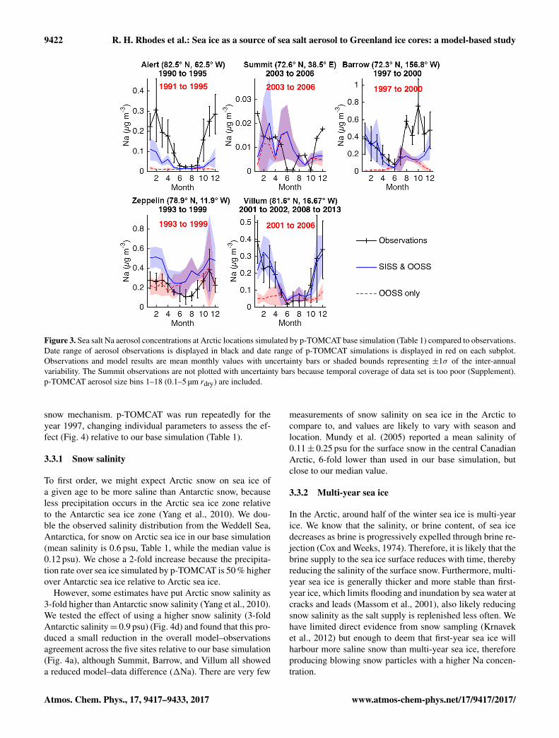
At the Arctic aerosol sampling sites, except Zeppelin, sim-ulated OOSS Na concentrations fall within the range of ob-servations in the summer months (Fig. 3). This suggests thatp-TOMCAT captures OOSS in the Arctic well, assuming themodel is accurate in simulating a minimal SISS contributionto the summer sea salt budget. Sensitivity tests show that theSST dependent OOSS emissions (Jaeglé et al., 2011) we usehere produces the best match between aerosol observationsand model simulations at Arctic sites. A small improvementmay be gained in future work using p-TOMCAT by adopt-ing the further modifications recently published by Haungand Jaeglé (2017), which restrict OOSS emissions at SSTs< 5 ◦C and in high-latitude grid squares with < 50 % watercoverage (Fig. S4).

3.3 Sea ice surface emissions

Results from our base simulation (Table 1) indicate that sim-ulated OOSS alone cannot reproduce the seasonal variabilityof aerosol Na observations at Arctic aerosol sites (Fig. 3).In the winter months, the simulated OOSS Na profiles showa deficit of Na relative to the observations. This is consis-tent with the idea that blowing snow from the sea ice surface(SISS) is an important source of sea salt to the Arctic andits inclusion in model studies is essential to replicate Arcticaerosol observations.

We now consider the influence of some of the various pa-rameters that can influence SISS emissions via the blowing

www.atmos-chem-phys.net/17/9417/2017/ Atmos. Chem. Phys., 17, 9417–9433, 2017

9422 R. H. Rhodes et al.: Sea ice as a source of sea salt aerosol to Greenland ice cores: a model-based study

Figure 3. Sea salt Na aerosol concentrations at Arctic locations simulated by p-TOMCAT base simulation (Table 1) compared to observations.Date range of aerosol observations is displayed in black and date range of p-TOMCAT simulations is displayed in red on each subplot.Observations and model results are mean monthly values with uncertainty bars or shaded bounds representing ±1σ of the inter-annualvariability. The Summit observations are not plotted with uncertainty bars because temporal coverage of data set is too poor (Supplement).p-TOMCAT aerosol size bins 1–18 (0.1–5 µm rdry) are included.

snow mechanism. p-TOMCAT was run repeatedly for theyear 1997, changing individual parameters to assess the ef-fect (Fig. 4) relative to our base simulation (Table 1).

3.3.1 Snow salinity

To first order, we might expect Arctic snow on sea ice ofa given age to be more saline than Antarctic snow, becauseless precipitation occurs in the Arctic sea ice zone relativeto the Antarctic sea ice zone (Yang et al., 2010). We dou-ble the observed salinity distribution from the Weddell Sea,Antarctica, for snow on Arctic sea ice in our base simulation(mean salinity is 0.6 psu, Table 1, while the median value is0.12 psu). We chose a 2-fold increase because the precipita-tion rate over sea ice simulated by p-TOMCAT is 50 % higherover Antarctic sea ice relative to Arctic sea ice.

However, some estimates have put Arctic snow salinity as3-fold higher than Antarctic snow salinity (Yang et al., 2010).We tested the effect of using a higher snow salinity (3-foldAntarctic salinity= 0.9 psu) (Fig. 4d) and found that this pro-duced a small reduction in the overall model–observationsagreement across the five sites relative to our base simulation(Fig. 4a), although Summit, Barrow, and Villum all showeda reduced model–data difference (1Na). There are very few

measurements of snow salinity on sea ice in the Arctic tocompare to, and values are likely to vary with season andlocation. Mundy et al. (2005) reported a mean salinity of0.11± 0.25 psu for the surface snow in the central CanadianArctic, 6-fold lower than used in our base simulation, butclose to our median value.

3.3.2 Multi-year sea ice

In the Arctic, around half of the winter sea ice is multi-yearice. We know that the salinity, or brine content, of sea icedecreases as brine is progressively expelled through brine re-jection (Cox and Weeks, 1974). Therefore, it is likely that thebrine supply to the sea ice surface reduces with time, therebyreducing the salinity of the surface snow. Furthermore, multi-year sea ice is generally thicker and more stable than first-year ice, which limits flooding and inundation by sea water atcracks and leads (Massom et al., 2001), also likely reducingsnow salinity as the salt supply is replenished less often. Wehave limited direct evidence from snow sampling (Krnaveket al., 2012) but enough to deem that first-year sea ice willharbour more saline snow than multi-year sea ice, thereforeproducing blowing snow particles with a higher Na concen-tration.

Atmos. Chem. Phys., 17, 9417–9433, 2017 www.atmos-chem-phys.net/17/9417/2017/

R. H. Rhodes et al.: Sea ice as a source of sea salt aerosol to Greenland ice cores: a model-based study 9423

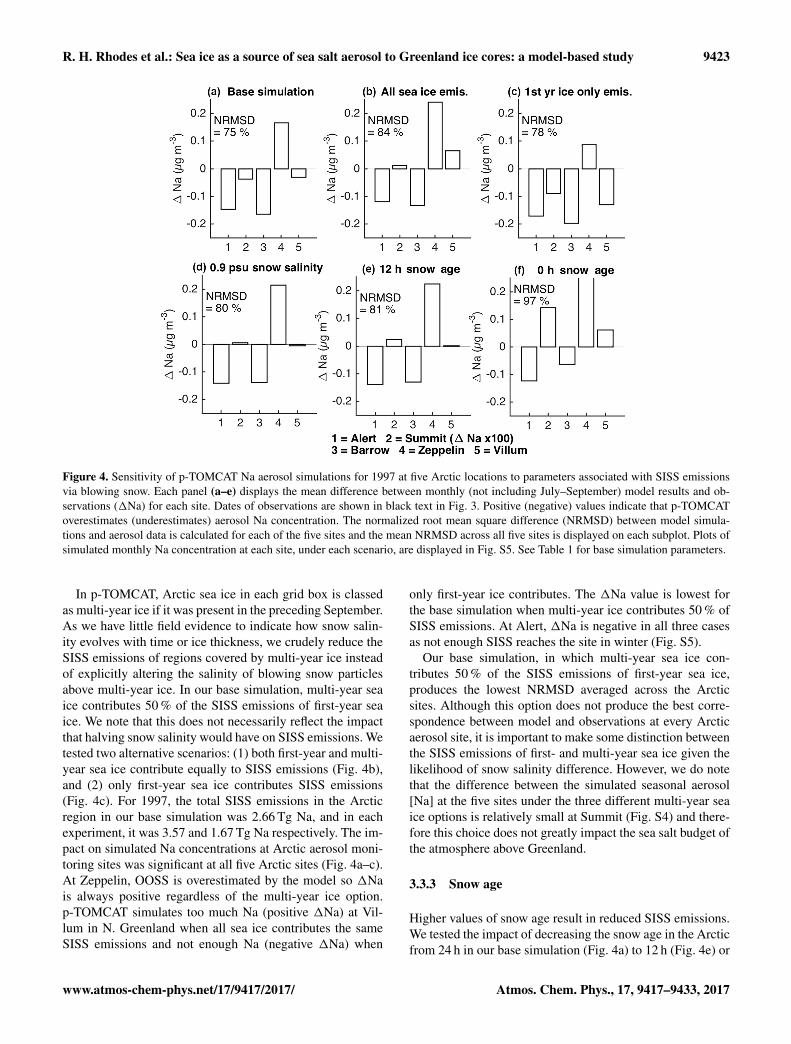
Figure 4. Sensitivity of p-TOMCAT Na aerosol simulations for 1997 at five Arctic locations to parameters associated with SISS emissionsvia blowing snow. Each panel (a–e) displays the mean difference between monthly (not including July–September) model results and ob-servations (1Na) for each site. Dates of observations are shown in black text in Fig. 3. Positive (negative) values indicate that p-TOMCAToverestimates (underestimates) aerosol Na concentration. The normalized root mean square difference (NRMSD) between model simula-tions and aerosol data is calculated for each of the five sites and the mean NRMSD across all five sites is displayed on each subplot. Plots ofsimulated monthly Na concentration at each site, under each scenario, are displayed in Fig. S5. See Table 1 for base simulation parameters.

In p-TOMCAT, Arctic sea ice in each grid box is classedas multi-year ice if it was present in the preceding September.As we have little field evidence to indicate how snow salin-ity evolves with time or ice thickness, we crudely reduce theSISS emissions of regions covered by multi-year ice insteadof explicitly altering the salinity of blowing snow particlesabove multi-year ice. In our base simulation, multi-year seaice contributes 50 % of the SISS emissions of first-year seaice. We note that this does not necessarily reflect the impactthat halving snow salinity would have on SISS emissions. Wetested two alternative scenarios: (1) both first-year and multi-year sea ice contribute equally to SISS emissions (Fig. 4b),and (2) only first-year sea ice contributes SISS emissions(Fig. 4c). For 1997, the total SISS emissions in the Arcticregion in our base simulation was 2.66 Tg Na, and in eachexperiment, it was 3.57 and 1.67 Tg Na respectively. The im-pact on simulated Na concentrations at Arctic aerosol moni-toring sites was significant at all five Arctic sites (Fig. 4a–c).At Zeppelin, OOSS is overestimated by the model so 1Nais always positive regardless of the multi-year ice option.p-TOMCAT simulates too much Na (positive 1Na) at Vil-lum in N. Greenland when all sea ice contributes the sameSISS emissions and not enough Na (negative 1Na) when

only first-year ice contributes. The 1Na value is lowest forthe base simulation when multi-year ice contributes 50 % ofSISS emissions. At Alert, 1Na is negative in all three casesas not enough SISS reaches the site in winter (Fig. S5).

Our base simulation, in which multi-year sea ice con-tributes 50 % of the SISS emissions of first-year sea ice,produces the lowest NRMSD averaged across the Arcticsites. Although this option does not produce the best corre-spondence between model and observations at every Arcticaerosol site, it is important to make some distinction betweenthe SISS emissions of first- and multi-year sea ice given thelikelihood of snow salinity difference. However, we do notethat the difference between the simulated seasonal aerosol[Na] at the five sites under the three different multi-year seaice options is relatively small at Summit (Fig. S4) and there-fore this choice does not greatly impact the sea salt budget ofthe atmosphere above Greenland.

3.3.3 Snow age

Higher values of snow age result in reduced SISS emissions.We tested the impact of decreasing the snow age in the Arcticfrom 24 h in our base simulation (Fig. 4a) to 12 h (Fig. 4e) or

www.atmos-chem-phys.net/17/9417/2017/ Atmos. Chem. Phys., 17, 9417–9433, 2017

9424 R. H. Rhodes et al.: Sea ice as a source of sea salt aerosol to Greenland ice cores: a model-based study

to zero (Fig. 4f) for 1997. For some sites, such as Barrowand Alert, 1Na was reduced with a snow age of 12 or 0 h(Fig. 4e and f compared to Fig. 4a). The model–observationsmatch across all the Arctic sites was reduced for both the12 h and zero snow age (NRMSD increased). If we excludeZeppelin from the calculation for 12 h snow age, the NRMSDis similar that achieved for the base simulation using a snowage of 24 h. The maximum change in monthly [Na] causedby setting the snow age to zero is a 70 % increase in [Na] atBarrow in January (Fig. S5).

3.4 Comparison between p-TOMCAT andGEOS-Chem

The performance of p-TOMCAT can be further evaluatedby comparing the simulation Arctic sea salt aerosol budgetto that reported by Huang and Jaeglé (2017), who use theGEOS-Chem model (Table 3). In order to make a direct com-parison with their reported values, Table 3 reports values for2005 only, which refer to sea salt aerosol, not just Na, and arefor the Arctic region only (note: lifetime in the Arctic region6= lifetime in the atmosphere).

For OOSS, the two models are broadly similar, witha tendency towards a higher burden, surface concen-tration, and Arctic lifetime in GEOS-Chem. For SISS,the emission rates are different between p-TOMCAT andGEOS-Chem. p-TOMCAT emits ∼ 5× more SISS in the0.57 µm<rdry≤ 4.5 µm range than GEOS-Chem, whileGEOS-Chem emits more than double the SISS of p-TOMCAT in the smaller particle size range. This differ-ence is due to the tuning introduced by Huang and Jaeglé(2017) that causes each snow particle to produce five sea saltaerosol (whereas in p-TOMCAT, one snow particle equalsone aerosol). The result is that deposition rates for large parti-cles in p-TOMCAT are proportionally greater, while the bur-den and surface concentration are quite similar between thetwo models. However, for the smaller particles, the surfaceconcentration and burden of sea salt are significantly lowerin p-TOMCAT, leading to an Arctic lifetime of 1.7 days ver-sus 6.6 days in GEOS-Chem.

Lack of observations of snow on sea ice in the Arctic, andof sea salt aerosol produced during blowing events, makes itdifficult to constrain many of the key parameters related tothe blowing snow SISS emission process. Although we usea snow salinity distribution double that of Antarctic observa-tions, a snow age of 24 h, and a 50 % reduction in SISS emis-sions from multi-year sea ice relative to first-year sea ice inour base simulation, we understand that a different combina-tion of these parameters could effectively produce the sameresults.

3.5 Importance of sea-ice-sourced sea salt aerosol

Despite the somewhat ambiguous choices of parameters thatwe have to make, it is important to note that in all the indi-

vidual sensitivity tests conducted for 1997, SISS contributesto offset the winter OOSS Na deficit at all five Arctic aerosolsites (Fig. S5). For the full base simulation, the addition ofSISS produces seasonal cycles that match well with overlap-ping Arctic aerosol observations. NRMSDs of between 34 %for Villum and 89 % for Alert (Fig. 3) are achieved. At Zep-pelin on Svalbard, the modelled OOSS contribution is toohigh throughout the year. However, the seasonal profile ofSISS looks promising – its amplitude is similar to the sea-sonal cycle of the observations. Villum, N. Greenland, showsthe best model–observations agreement, with SISS contribut-ing 80 % of the total Na in the winter months on average.Results for Barrow, Alaska, are equally encouraging for Jan-uary to June, but p-TOMCAT appears to underestimate SISSin the latter half of the year, hinting that SISS emission ratesmay vary with the cycle of sea ice decay and regrowth.

Only Alert, Canada, shows a significant offset betweenthe aerosol observations and the modelled Na concentration(Fig. 3). The summer concentrations, dominated by OOSSmatch well, but in other months p-TOMCAT underestimates[Na]. Huang and Jaeglé (2017) had a similar problem es-timating aerosol [Na] at Alert and suggested that it resultsfrom Alert being situated in a region of relatively calm andstable meteorological conditions where the threshold windspeed (∼ 7 m s−1) for SISS emissions is not reached as of-ten. Huang and Jaeglé (2017) found that the inclusion of anexplicitly parameterized frost flower source (Xu et al., 2013)helped to match the observed sea salt aerosol budget at Alert.Further field measurements are required to assess to what ex-tent frost flowers do actually contribute aerosol to the atmo-spheric sea salt budget at low wind speeds, given evidence tothe contrary (Obbard et al., 2009; Roscoe et al., 2011; Yanget al., 2017).

The simulated seasonal Na aerosol cycle for Summit,Greenland, matches the aerosol observations well (Fig. 3).Our results suggest that OOSS is the dominant source ofNa to the high-altitude central interior of the Greenland icesheet with significant SISS Na only present from Novemberto March, contributing a maximum of 44 % of the monthlyNa budget.

4 Comparison of p-TOMCAT simulations to ice coreNa records

We now examine our p-TOMCAT base simulation (Table 1)of deposited sea salt for 1991–1999 to investigate the contri-bution of SISS to sea salt concentrations of Greenland icecore records. All the ice cores we consider are located at> 2000 m elevation and > 100 km inland (Table 2) so max-imum Na concentrations are < 100 ppb. Seasonal variabilityin [Na] is consistently characterized by winter maxima andsummer minima (Fig. 5); the amplitude of the mean seasonalcycle in the different ice cores varies between 6 and 55 ppb.

Atmos. Chem. Phys., 17, 9417–9433, 2017 www.atmos-chem-phys.net/17/9417/2017/

R. H. Rhodes et al.: Sea ice as a source of sea salt aerosol to Greenland ice cores: a model-based study 9425

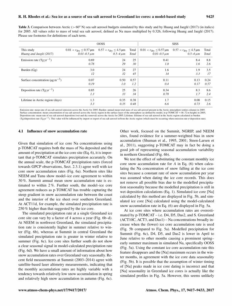
Table 3. Comparison between Arctic (> 60◦ N) sea salt aerosol budgets simulated by this study and by Huang and Jaeglé (2017) (in italics)for 2005. All values refer to mass of total sea salt aerosol, defined as Na mass multiplied by 0.326, following Huang and Jaeglé (2017).Please see footnotes for definitions of each term.

OOSS SISS

This study 0.01< rdry ≤ 0.57 µm 0.57< rdry ≤ 4.5 µm Total 0.01< rdry ≤ 0.57 µm 0.57< rdry ≤ 4.5 µm TotalHuang and Jaeglé (2017) 0.01–0.5µm 0.5–4µm Total 0.01–0.5µm 0.5–4µm Total

Emission rate (Tg yr−1) 0.69 24 25 0.41 8.4 8.80.78 29 30 1.0 1.6 2.6

Burden (Gg) 3.0 24 27 1.6 1.9 3.512 32 45 14 3.3 17

Surface concentration (µg m−3) 0.07 0.50 0.57 0.11 0.13 0.240.19 1.0 1.2 0.4 0.17 0.57

Deposition rate (Tg yr−1) 0.85 25 26 0.34 8.3 8.61.3 33 34 0.78 1.7 2.4

Lifetime in Arctic region (days) 1.3 0.35 0.38 1.7 0.08 0.153.3 0.35 0.48 6.6 0.73 2.6

Emission rate: mean rate of sea salt aerosol emission across the Arctic for 2005; Burden: annual mean total mass of sea salt aerosol present in the Arctic atmosphere (entire column) in 2005.Surface concentration: mean concentration of sea salt aerosol across the Arctic region in the surface layer of the atmosphere (as defined by model, in p-TOMCAT ≈ 46–72 m height) in 2005;Deposition rate: mean rate of sea salt aerosol deposition (wet and dry removal) across the Arctic for 2005; Lifetime: lifetime of sea salt aerosol in the Arctic region calculated as burden(Tg)/deposition rate (Tg yr−1). This value will be influenced by import or export of sea salt aerosol to/from the Arctic region (which must be occurring when emission rate 6= deposition rate).

4.1 Influence of snow accumulation rate

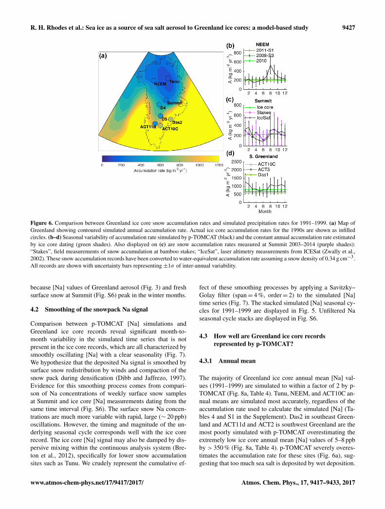
Given that simulation of ice core Na concentrations usingp-TOMCAT requires both the mass of Na deposited and theamount of precipitation at the ice core site (Eq. 6), it is impor-tant that p-TOMCAT simulates precipitation accurately. Onthe annual scale, the p-TOMCAT precipitation rates (forcedtowards GPCP observations, Sect. 2.3.1) agree well with icecore snow accumulation rates (Fig. 6a). Northern sites likeNEEM and Tunu show model–ice core agreement to within30 %. Summit annual mean snow accumulation rate is es-timated to within 2 %. Further south, the model–ice coreagreement reduces as p-TOMCAT has trouble capturing thesteep gradient in snow accumulation rate between the coastand the interior of the ice sheet over southern Greenland.At ACT11d, for example, the simulated precipitation rate is250 % higher than that suggested by the ice core.

The simulated precipitation rate at a single Greenland icecore site can vary by a factor of 4 across a year (Fig. 6b–d).At NEEM in northwest Greenland, the simulated precipita-tion rate is consistently higher in summer relative to win-ter (Fig. 6b), whereas at Summit in central Greenland thesimulated precipitation rate is greater in winter relative tosummer (Fig. 6c). Ice core sites further south do not showa clear seasonal signal in model-calculated precipitation rate(Fig. 6d). We have a small amount of information about howsnow accumulation rates over Greenland vary seasonally. Re-cent field measurements at Summit (2003–2014) agree withsatellite-based laser altimetry measurements, indicating thatthe monthly accumulation rates are highly variable with atendency towards relatively low snow accumulation in springand relatively high snow accumulation in autumn (Fig. 6c).

Other work, focused on the Summit, NGRIP, and NEEMsites, found evidence for a summer-weighted bias in snowaccumulation (Shuman et al., 1995, 2001; Steen-Larsen etal., 2011), suggesting p-TOMCAT may in fact be doing agood job of representing seasonal accumulation variabilityin northern Greenland (Fig. 6b).

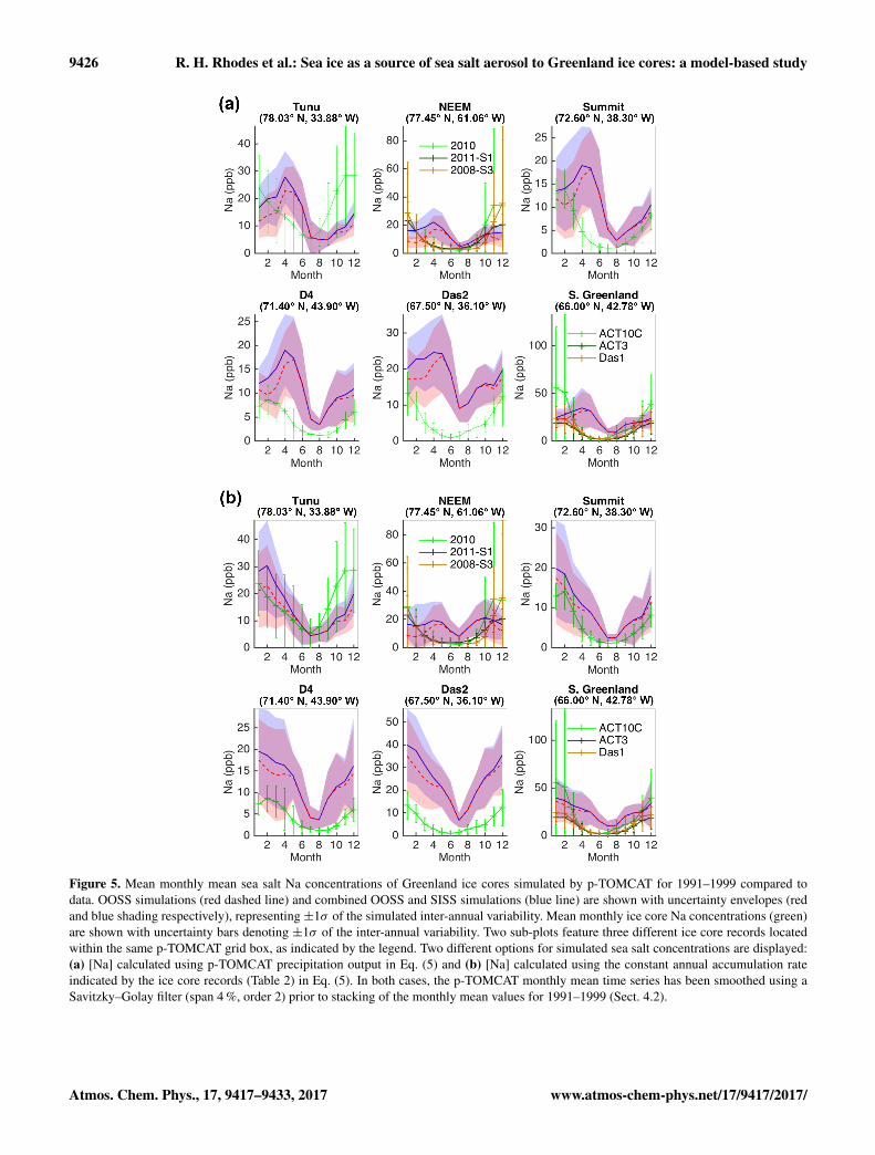
We test the effect of substituting the constant monthly icecore snow accumulation rate for A in Eq. (6) when calcu-lating the Na concentration of snow falling at the ice coresites because a constant rate of snow accumulation per yearwas assumed when dating the ice core records. This doesnot remove all possible bias due to the modelled precipita-tion seasonality because the modelled precipitation is still inwet deposition calculations (Eq. 1). Simulated ice core [Na]calculated by this method are displayed in Fig. 5b, and sim-ulated ice core [Na] calculated using the model-calculatedsnow accumulation rate in Eq. (6) are displayed in Fig. 5a.

At ice core sites where accumulation rates are overesti-mated by p-TOMCAT – i.e. D4, D5, Das2, and S. Greenland(ACT10C, ACT3, and Das1) – Na concentrations broadly in-crease when the (lower) ice core accumulation rate is used(Fig. 5b compared to Fig. 5a). Modelled precipitation forSummit (Fig. 6c), D4, D5, and Das2 is lower in April toJune relative to other months causing a prominent spring–early summer maximum in simulated Na, specifically OOSS(Fig. 5a). Using the constant ice core accumulation rate thisfeature disappears and the [Na] maximum occurs in the win-ter months, in agreement with the ice core data seasonality(Fig. 5b). It is possible that the assumption of winter timingof [Na] peaks made in ice core dating is incorrect and that[Na] seasonality in Greenland ice cores is actually like thesimulated profiles in Fig. 5a. However, this seems unlikely

www.atmos-chem-phys.net/17/9417/2017/ Atmos. Chem. Phys., 17, 9417–9433, 2017

9426 R. H. Rhodes et al.: Sea ice as a source of sea salt aerosol to Greenland ice cores: a model-based study

Figure 5. Mean monthly mean sea salt Na concentrations of Greenland ice cores simulated by p-TOMCAT for 1991–1999 compared todata. OOSS simulations (red dashed line) and combined OOSS and SISS simulations (blue line) are shown with uncertainty envelopes (redand blue shading respectively), representing ±1σ of the simulated inter-annual variability. Mean monthly ice core Na concentrations (green)are shown with uncertainty bars denoting ±1σ of the inter-annual variability. Two sub-plots feature three different ice core records locatedwithin the same p-TOMCAT grid box, as indicated by the legend. Two different options for simulated sea salt concentrations are displayed:(a) [Na] calculated using p-TOMCAT precipitation output in Eq. (5) and (b) [Na] calculated using the constant annual accumulation rateindicated by the ice core records (Table 2) in Eq. (5). In both cases, the p-TOMCAT monthly mean time series has been smoothed using aSavitzky–Golay filter (span 4 %, order 2) prior to stacking of the monthly mean values for 1991–1999 (Sect. 4.2).

Atmos. Chem. Phys., 17, 9417–9433, 2017 www.atmos-chem-phys.net/17/9417/2017/

R. H. Rhodes et al.: Sea ice as a source of sea salt aerosol to Greenland ice cores: a model-based study 9427

Figure 6. Comparison between Greenland ice core snow accumulation rates and simulated precipitation rates for 1991–1999. (a) Map ofGreenland showing contoured simulated annual accumulation rate. Actual ice core accumulation rates for the 1990s are shown as infilledcircles. (b–d) Seasonal variability of accumulation rate simulated by p-TOMCAT (black) and the constant annual accumulation rate estimatedby ice core dating (green shades). Also displayed on (c) are snow accumulation rates measured at Summit 2003–2014 (purple shades):“Stakes”, field measurements of snow accumulation at bamboo stakes; “IceSat”, laser altimetry measurements from ICESat (Zwally et al.,2002). These snow accumulation records have been converted to water-equivalent accumulation rate assuming a snow density of 0.34 g cm−3.All records are shown with uncertainty bars representing ±1σ of inter-annual variability.

because [Na] values of Greenland aerosol (Fig. 3) and freshsurface snow at Summit (Fig. S6) peak in the winter months.

4.2 Smoothing of the snowpack Na signal

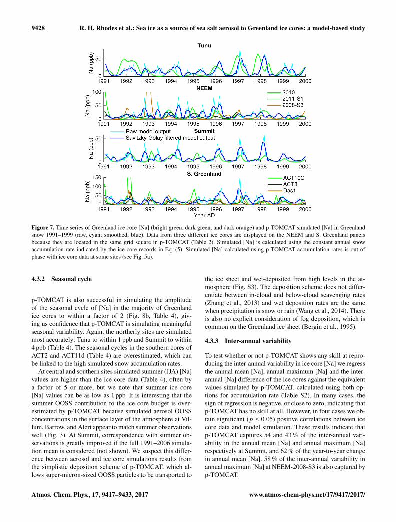
Comparison between p-TOMCAT [Na] simulations andGreenland ice core records reveal significant month-to-month variability in the simulated time series that is notpresent in the ice core records, which are all characterized bysmoothly oscillating [Na] with a clear seasonality (Fig. 7).We hypothesize that the deposited Na signal is smoothed bysurface snow redistribution by winds and compaction of thesnow pack during densification (Dibb and Jaffrezo, 1997).Evidence for this smoothing process comes from compari-son of Na concentrations of weekly surface snow samplesat Summit and ice core [Na] measurements dating from thesame time interval (Fig. S6). The surface snow Na concen-trations are much more variable with rapid, large (∼ 20 ppb)oscillations. However, the timing and magnitude of the un-derlying seasonal cycle corresponds well with the ice corerecord. The ice core [Na] signal may also be damped by dis-persive mixing within the continuous analysis system (Bre-ton et al., 2012), specifically for lower snow accumulationsites such as Tunu. We crudely represent the cumulative ef-

fect of these smoothing processes by applying a Savitzky–Golay filter (span= 4 %, order= 2) to the simulated [Na]time series (Fig. 7). The stacked simulated [Na] seasonal cy-cles for 1991–1999 are displayed in Fig. 5. Unfiltered Naseasonal cycle stacks are displayed in Fig. S6.

4.3 How well are Greenland ice core recordsrepresented by p-TOMCAT?

4.3.1 Annual mean

The majority of Greenland ice core annual mean [Na] val-ues (1991–1999) are simulated to within a factor of 2 by p-TOMCAT (Fig. 8a, Table 4). Tunu, NEEM, and ACT10C an-nual means are simulated most accurately, regardless of theaccumulation rate used to calculate the simulated [Na] (Ta-bles 4 and S1 in the Supplement). Das2 in southeast Green-land and ACT11d and ACT2 is southwest Greenland are themost poorly simulated with p-TOMCAT overestimating theextremely low ice core annual mean [Na] values of 5–8 ppbby > 350 % (Fig. 8a, Table 4). p-TOMCAT severely overes-timates the accumulation rate for these sites (Fig. 6a), sug-gesting that too much sea salt is deposited by wet deposition.

www.atmos-chem-phys.net/17/9417/2017/ Atmos. Chem. Phys., 17, 9417–9433, 2017

9428 R. H. Rhodes et al.: Sea ice as a source of sea salt aerosol to Greenland ice cores: a model-based study

Figure 7. Time series of Greenland ice core [Na] (bright green, dark green, and dark orange) and p-TOMCAT simulated [Na] in Greenlandsnow 1991–1999 (raw, cyan; smoothed, blue). Data from three different ice cores are displayed on the NEEM and S. Greenland panelsbecause they are located in the same grid square in p-TOMCAT (Table 2). Simulated [Na] is calculated using the constant annual snowaccumulation rate indicated by the ice core records in Eq. (5). Simulated [Na] calculated using p-TOMCAT accumulation rates is out ofphase with ice core data at some sites (see Fig. 5a).

4.3.2 Seasonal cycle

p-TOMCAT is also successful in simulating the amplitudeof the seasonal cycle of [Na] in the majority of Greenlandice cores to within a factor of 2 (Fig. 8b, Table 4), giv-ing us confidence that p-TOMCAT is simulating meaningfulseasonal variability. Again, the northerly sites are simulatedmost accurately: Tunu to within 1 ppb and Summit to within4 ppb (Table 4). The seasonal cycles in the southern cores ofACT2 and ACT11d (Table 4) are overestimated, which canbe linked to the high simulated snow accumulation rates.

At central and southern sites simulated summer (JJA) [Na]values are higher than the ice core data (Table 4), often bya factor of 5 or more, but we note that summer ice core[Na] values can be as low as 1 ppb. It is interesting that thesummer OOSS contribution to the ice core budget is over-estimated by p-TOMCAT because simulated aerosol OOSSconcentrations in the surface layer of the atmosphere at Vil-lum, Barrow, and Alert appear to match summer observationswell (Fig. 3). At Summit, correspondence with summer ob-servations is greatly improved if the full 1991–2006 simula-tion mean is considered (not shown). We suspect this differ-ence between aerosol and ice core simulations results fromthe simplistic deposition scheme of p-TOMCAT, which al-lows super-micron-sized OOSS particles to be transported to

the ice sheet and wet-deposited from high levels in the at-mosphere (Fig. S3). The deposition scheme does not differ-entiate between in-cloud and below-cloud scavenging rates(Zhang et al., 2013) and wet deposition rates are the samewhen precipitation is snow or rain (Wang et al., 2014). Thereis also no explicit consideration of fog deposition, which iscommon on the Greenland ice sheet (Bergin et al., 1995).

4.3.3 Inter-annual variability

To test whether or not p-TOMCAT shows any skill at repro-ducing the inter-annual variability in ice core [Na] we regressthe annual mean [Na], annual maximum [Na] and the inter-annual [Na] difference of the ice cores against the equivalentvalues simulated by p-TOMCAT, calculated using both op-tions for accumulation rate (Table S2). In many cases, thesign of regression is negative, or close to zero, indicating thatp-TOMCAT has no skill at all. However, in four cases we ob-tain significant (p ≤ 0.05) positive correlations between icecore data and model simulation. These results indicate thatp-TOMCAT captures 54 and 43 % of the inter-annual vari-ability in the annual mean [Na] and annual maximum [Na]respectively at Summit, and 62 % of the year-to-year changein annual mean [Na]. 58 % of the inter-annual variability inannual maximum [Na] at NEEM-2008-S3 is also captured byp-TOMCAT.

Atmos. Chem. Phys., 17, 9417–9433, 2017 www.atmos-chem-phys.net/17/9417/2017/

R. H. Rhodes et al.: Sea ice as a source of sea salt aerosol to Greenland ice cores: a model-based study 9429

Table 4. Mean sea salt Na concentrations for 1991–1999 recordedin ice cores (bold) and simulated by p-TOMCAT calculated usingmodelled precipitation rates in Eq. (5). See Table S1 for equivalentvalues calculated using ice core snow accumulation rates.

Ice coreAnnual DJF JJA Seasonal DJF

[Na] [Na] [Na] cycle [Na]a SISS :(ppb) (ppb) (ppb) (ppb) OOSS

Tunu 16 24 7 2214 17 9 23 0.4

NEEM-2008-S3 11 25 3 3114 16 7 17 1.0

Summit 6 12 1 1311 13 7 16 0.2

D4 4 8 1 811 12 7 16 0.2

D5 8 13 4 1014 16 8 19 0.2

Das2 5 12 2 1218 21 13 16 0.2

Das1b 11 23 2 2322 25 13 25 0.1

ACT10Cb 21 49 4 5522 25 13 25 0.1

ACT3b 9 19 2 1822 25 13 25 0.1

ACT2c 8 13 3 1025 24 16 31 0.1

ACT11dc 7 10 5 725 24 16 31 0.1

a Seasonal cycle is the maximum monthly mean [Na] minus the minimum monthly mean[Na]. b Same grid square in p-TOMCAT so simulated values are equal. c Same grid square inp-TOMCAT so simulated values are equal.

These results are promising, given that 1991 to 1999 isa relatively short time series for comparison. Additionally,it is unlikely that a chemical transport model could explaina greater proportion of inter-annual variability in ice core[Na] than achieved here. This is because ice core chemistryrecords are affected by several factors that impact the finalrecord preserved, in addition to the meteorology and sourceconditions parameterized by p-TOMCAT. Factors such assnow redistribution and wind-generated features such as sas-trugi can cause chemistry (Gfeller et al., 2014) and accu-mulation rate (Mosley-Thompson et al., 2001) records fromproximal ice cores to differ; Dibb and Jaffrezo (1997) foundannual mean [Na] of the snowpack at Greenland varied byup 30 % between sites < 1 km apart. We can see that this isthe case by comparing the different NEEM ice core recordsor S. Greenland ice core records in Fig. 5 or 7 that show sig-nificant differences in [Na] despite being located in the samep-TOMCAT grid box.

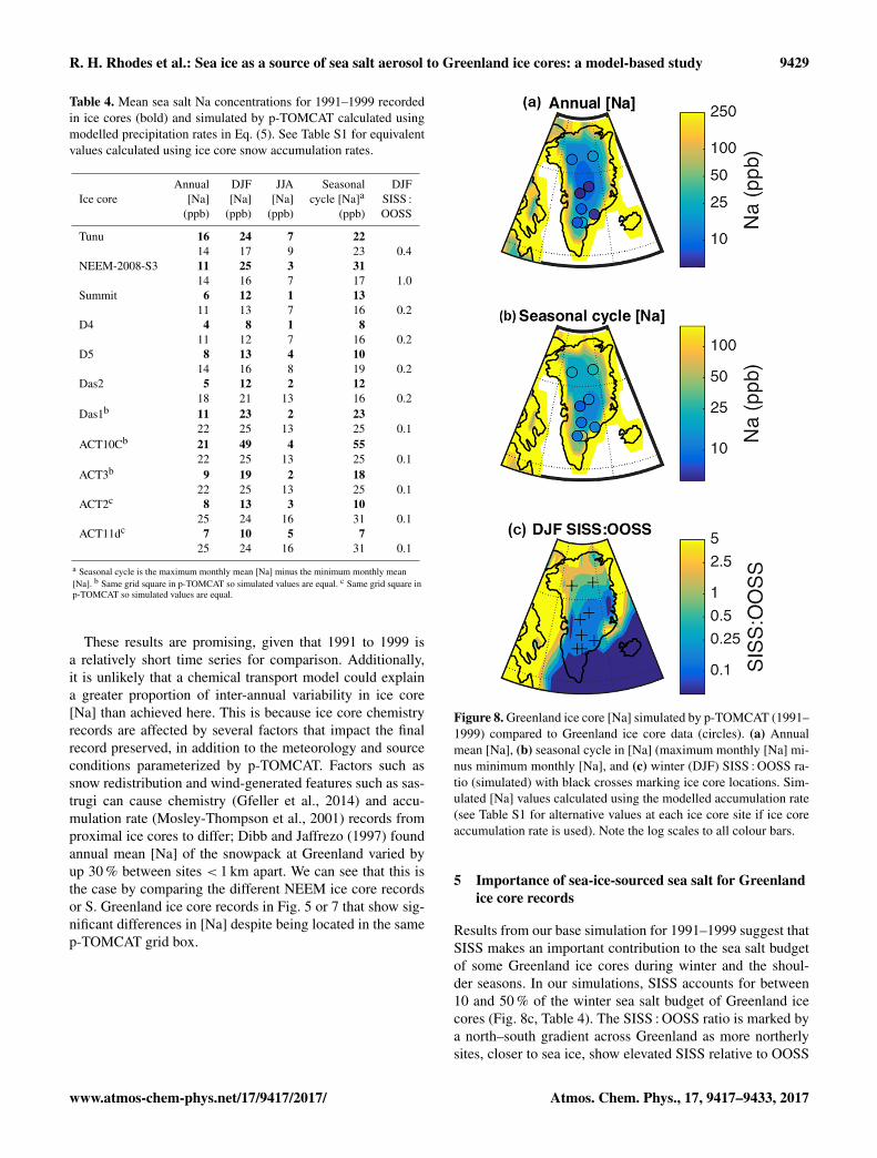
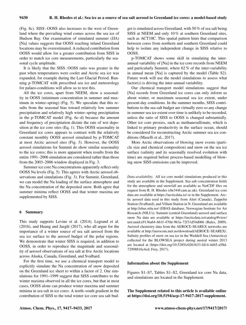
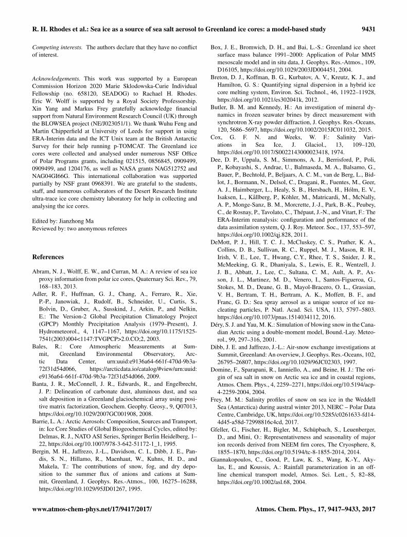
Figure 8. Greenland ice core [Na] simulated by p-TOMCAT (1991–1999) compared to Greenland ice core data (circles). (a) Annualmean [Na], (b) seasonal cycle in [Na] (maximum monthly [Na] mi-nus minimum monthly [Na], and (c) winter (DJF) SISS : OOSS ra-tio (simulated) with black crosses marking ice core locations. Sim-ulated [Na] values calculated using the modelled accumulation rate(see Table S1 for alternative values at each ice core site if ice coreaccumulation rate is used). Note the log scales to all colour bars.

5 Importance of sea-ice-sourced sea salt for Greenlandice core records

Results from our base simulation for 1991–1999 suggest thatSISS makes an important contribution to the sea salt budgetof some Greenland ice cores during winter and the shoul-der seasons. In our simulations, SISS accounts for between10 and 50 % of the winter sea salt budget of Greenland icecores (Fig. 8c, Table 4). The SISS : OOSS ratio is marked bya north–south gradient across Greenland as more northerlysites, closer to sea ice, show elevated SISS relative to OOSS

www.atmos-chem-phys.net/17/9417/2017/ Atmos. Chem. Phys., 17, 9417–9433, 2017

9430 R. H. Rhodes et al.: Sea ice as a source of sea salt aerosol to Greenland ice cores: a model-based study

(Fig. 8c). SISS : OOSS also increases to the west of Green-land where the prevailing wind comes across the sea ice ofHudson Bay. Our examination of simulated summer (JJA)[Na] values suggests that OOSS reaching inland Greenlandlocations may be overestimated. A reduced contribution fromOOSS would allow for a greater contribution from SISS inorder to match ice core measurements, particularly the sea-sonal cycle amplitude.

It is likely that the SISS : OOSS ratio was greater in thepast when temperatures were cooler and Arctic sea ice wasexpanded, for example during the Last Glacial Period. Run-ning p-TOMCAT with prescribed sea ice and meteorologyfor palaeo-conditions will allow us to test this.

All the ice cores, apart from NEEM, show a seasonal-ity in OOSS (minimum concentration in summer and max-imum in winter–spring) (Fig. 5). We speculate that this re-sults from the seasonal bias toward relatively low summerprecipitation and relatively high winter–spring precipitationin the p-TOMCAT model (Fig. 6c–d) because the amountand frequency of precipitation dictate the rate of wet depo-sition at the ice core sites (Eq. 1). This OOSS seasonality inGreenland ice cores appears to contrast with the relativelyconstant monthly OOSS aerosol simulated by p-TOMCATat most Arctic aerosol sites (Fig. 3). However, the OOSSaerosol simulations for Summit do show similar seasonalityto the ice cores; this is more apparent when results from theentire 1991–2006 simulation are considered rather than thosefrom the 2003–2006 window displayed in Fig. 3.

Summer ice core Na concentrations apparently reflect onlyOOSS Na levels (Fig. 5). This agrees with Arctic aerosol ob-servations and simulations (Fig. 3). For Summit, Greenland,we can model the Na loading of the surface atmosphere andthe Na concentration of the deposited snow. Both agree thatsummer minima reflect OOSS and that winter maxima aresupplemented by SISS.

6 Summary

This study supports Levine et al. (2014), Legrand et al.(2016), and Huang and Jaeglé (2017), who all argue for theimportance of a winter source of sea salt aerosol from thesea ice surface to the aerosol budget of the polar regions.We demonstrate that winter SISS is required, in addition toOOSS, in order to reproduce the magnitude and seasonal-ity of aerosol observations of sea salt at five Arctic locationsacross Alaska, Canada, Greenland, and Svalbard.

For the first time, we use a chemical transport model toexplicitly simulate the Na concentration of snow depositedon the Greenland ice sheet to within a factor of 2. Our sim-ulations for 1991–1999 suggest that SISS contributes to thewinter maxima observed in all the ice cores, but that in mostcases, OOSS alone can produce winter maxima and summerminima in sea salt in ice cores. A north–south gradient in thecontribution of SISS to the total winter ice core sea salt bud-

get is simulated across Greenland, with 50 % of sea salt beingSISS at NEEM and only 10 % at southern Greenland sites,such as ACT10C. This spatial pattern hints that comparisonbetween cores from northern and southern Greenland couldhelp to isolate any independent change in SISS relative toOOSS.

p-TOMCAT shows some skill in simulating the inter-annual variability of [Na] in the ice core records from NEEMand particularly Summit, where 62 % of the inter-variabilityin annual mean [Na] is captured by the model (Table S2).Future work will use the model simulations to assess whatfactor(s) is driving the inter-annual variability.

Our chemical transport model simulations suggest that[Na] records from Greenland ice cores can only inform usabout winter, or maximum seasonal sea ice extent, underpresent-day conditions. In the summer months, SISS contri-butions to the sea salt budget are virtually zero so any changein summer sea ice extent over time is unlikely to be recorded,unless the ratio of SISS to OOSS is changed substantially.Other ice core proxies, such as methanesulfonate, which islinked to primary productivity in the surface ocean, shouldbe considered for reconstructing Arctic summer sea ice con-ditions (Maselli et al., 2017).

More Arctic observations of blowing snow events (parti-cle size and chemical composition) and snow on the sea icesurface (salinity and its seasonally resolved evolution withtime) are required before process-based modelling of blow-ing snow SISS emissions can be improved.

Data availability. All ice core model simulations produced in thisstudy are available in the Supplement. Sea salt concentration fieldsfor the atmosphere and snowfall are available as NetCDF files onrequest from R. H. Rhodes (rhr34@cam.ac.uk). Greenland ice coredata are available at https://arcticdata.io/ or in the Supplement. Arc-tic aerosol data used in this study from Alert (Canada), ZeppelinStation (Svalbard), and Villum Station in N. Greenland are availableat http://ebas.nilu.no/ (EBAS database, Norwegian Institute for AirResearch (NILU)). Summit (central Greenland) aerosol and surfacesnow Na data are available at https://arcticdata.io/catalog/#view/urn:uuid:e9136a64-661f-470d-9b3a-72f31d54d066 (Bales, 2009).Aerosol chemistry data from the AEROCE-SEAREX networks areavailable at http://aerocom.met.no/download/AEROCE-SEAREX/.Salinity profiles of snow on sea ice in the Weddell Sea (Antarctica)collected for the BLOWSEA project during austral winter 2013are located at (https://doi.org/10.5285/c0261633-fd14-4d45-a58d-72998816c4cd; Frey, 2017).

Information about the Supplement

Figures S1–S7, Tables S1–S2, Greenland ice core Na data,and simulations are located in the Supplement.

The Supplement related to this article is available onlineat https://doi.org/10.5194/acp-17-9417-2017-supplement.

Atmos. Chem. Phys., 17, 9417–9433, 2017 www.atmos-chem-phys.net/17/9417/2017/

R. H. Rhodes et al.: Sea ice as a source of sea salt aerosol to Greenland ice cores: a model-based study 9431

Competing interests. The authors declare that they have no conflictof interest.

Acknowledgements. This work was supported by a EuropeanCommission Horizon 2020 Marie Sklodowska-Curie IndividualFellowship (no. 658120, SEADOG) to Rachael H. Rhodes.Eric W. Wolff is supported by a Royal Society Professorship.Xin Yang and Markus Frey gratefully acknowledge financialsupport from Natural Environment Research Council (UK) throughthe BLOWSEA project (NE/J023051/1). We thank Wuhu Feng andMartin Chipperfield at University of Leeds for support in usingERA-Interim data and the ICT Unix team at the British AntarcticSurvey for their help running p-TOMCAT. The Greenland icecores were collected and analysed under numerous NSF Officeof Polar Programs grants, including 021515, 0856845, 0909499,0909499, and 1204176, as well as NASA grants NAG512752 andNAG04GI66G. This international collaboration was supportedpartially by NSF grant 0968391. We are grateful to the students,staff, and numerous collaborators of the Desert Research Instituteultra-trace ice core chemistry laboratory for help in collecting andanalysing the ice cores.

Edited by: Jianzhong MaReviewed by: two anonymous referees

References

Abram, N. J., Wolff, E. W., and Curran, M. A.: A review of sea iceproxy information from polar ice cores, Quaternary Sci. Rev., 79,168–183, 2013.

Adler, R. F., Huffman, G. J., Chang, A., Ferraro, R., Xie,P.-P., Janowiak, J., Rudolf, B., Schneider, U., Curtis, S.,Bolvin, D., Gruber, A., Susskind, J., Arkin, P., and Nelkin,E.: The Version-2 Global Precipitation Climatology Project(GPCP) Monthly Precipitation Analysis (1979–Present), J.Hydrometeorol., 4, 1147–1167, https://doi.org/10.1175/1525-7541(2003)004<1147:TVGPCP>2.0.CO;2, 2003.

Bales, R.: Core Atmospheric Measurements at Sum-mit, Greenland Environmental Observatory, Arc-tic Data Center, urn:uuid:e9136a64-661f-470d-9b3a-72f31d54d066, https://arcticdata.io/catalog/#view/urn:uuid:e9136a64-661f-470d-9b3a-72f31d54d066, 2009.

Banta, J. R., McConnell, J. R., Edwards, R., and Engelbrecht,J. P.: Delineation of carbonate dust, aluminous dust, and seasalt deposition in a Greenland glaciochemical array using posi-tive matrix factorization, Geochem. Geophy. Geosy., 9, Q07013,https://doi.org/10.1029/2007GC001908, 2008.

Barrie, L. A.: Arctic Aerosols: Composition, Sources and Transport,in: Ice Core Studies of Global Biogeochemical Cycles, edited by:Delmas, R. J., NATO ASI Series, Springer Berlin Heidelberg, 1–22, https://doi.org/10.1007/978-3-642-51172-1_1, 1995.

Bergin, M. H., Jaffrezo, J.-L., Davidson, C. I., Dibb, J. E., Pan-dis, S. N., Hillamo, R., Maenhaut, W., Kuhns, H. D., andMakela, T.: The contributions of snow, fog, and dry depo-sition to the summer flux of anions and cations at Sum-mit, Greenland, J. Geophys. Res.-Atmos., 100, 16275–16288,https://doi.org/10.1029/95JD01267, 1995.

Box, J. E., Bromwich, D. H., and Bai, L.-S.: Greenland ice sheetsurface mass balance 1991–2000: Application of Polar MM5mesoscale model and in situ data, J. Geophys. Res.-Atmos., 109,D16105, https://doi.org/10.1029/2003JD004451, 2004.

Breton, D. J., Koffman, B. G., Kurbatov, A. V., Kreutz, K. J., andHamilton, G. S.: Quantifying signal dispersion in a hybrid icecore melting system, Environ. Sci. Technol., 46, 11922–11928,https://doi.org/10.1021/es302041k, 2012.

Butler, B. M. and Kennedy, H.: An investigation of mineral dy-namics in frozen seawater brines by direct measurement withsynchrotron X-ray powder diffraction, J. Geophys. Res.-Oceans,120, 5686–5697, https://doi.org/10.1002/2015JC011032, 2015.

Cox, G. F. N. and Weeks, W. F.: Salinity Vari-ations in Sea Ice, J. Glaciol., 13, 109–120,https://doi.org/10.1017/S0022143000023418, 1974.

Dee, D. P., Uppala, S. M., Simmons, A. J., Berrisford, P., Poli,P., Kobayashi, S., Andrae, U., Balmaseda, M. A., Balsamo, G.,Bauer, P., Bechtold, P., Beljaars, A. C. M., van de Berg, L., Bid-lot, J., Bormann, N., Delsol, C., Dragani, R., Fuentes, M., Geer,A. J., Haimberger, L., Healy, S. B., Hersbach, H., Hólm, E. V.,Isaksen, L., Kållberg, P., Köhler, M., Matricardi, M., McNally,A. P., Monge-Sanz, B. M., Morcrette, J.-J., Park, B.-K., Peubey,C., de Rosnay, P., Tavolato, C., Thépaut, J.-N., and Vitart, F.: TheERA-Interim reanalysis: configuration and performance of thedata assimilation system, Q. J. Roy. Meteor. Soc., 137, 553–597,https://doi.org/10.1002/qj.828, 2011.

DeMott, P. J., Hill, T. C. J., McCluskey, C. S., Prather, K. A.,Collins, D. B., Sullivan, R. C., Ruppel, M. J., Mason, R. H.,Irish, V. E., Lee, T., Hwang, C.Y., Rhee, T. S., Snider, J. R.,McMeeking, G. R., Dhaniyala, S., Lewis, E. R., Wentzell, J.J. B., Abbatt, J., Lee, C., Sultana, C. M., Ault, A. P., Ax-son, J. L., Martinez, M. D., Venero, I., Santos-Figueroa, G.,Stokes, M. D., Deane, G. B., Mayol-Bracero, O. L., Grassian,V. H., Bertram, T. H., Bertram, A. K., Moffett, B. F., andFranc, G. D.: Sea spray aerosol as a unique source of ice nu-cleating particles, P. Natl. Acad. Sci. USA, 113, 5797–5803.https://doi.org/10.1073/pnas.1514034112, 2016.

Déry, S. J. and Yau, M. K.: Simulation of blowing snow in the Cana-dian Arctic using a double-moment model, Bound.-Lay. Meteo-rol., 99, 297–316, 2001.

Dibb, J. E. and Jaffrezo, J.-L.: Air-snow exchange investigations atSummit, Greenland: An overview, J. Geophys. Res.-Oceans, 102,26795–26807, https://doi.org/10.1029/96JC02303, 1997.

Domine, F., Sparapani, R., Ianniello, A., and Beine, H. J.: The ori-gin of sea salt in snow on Arctic sea ice and in coastal regions,Atmos. Chem. Phys., 4, 2259–2271, https://doi.org/10.5194/acp-4-2259-2004, 2004.

Frey, M. M.: Salinity profiles of snow on sea ice in the WeddellSea (Antarctica) during austral winter 2013, NERC – Polar DataCentre, Cambridge, UK, https://doi.org/10.5285/c0261633-fd14-4d45-a58d-72998816c4cd, 2017.

Gfeller, G., Fischer, H., Bigler, M., Schüpbach, S., Leuenberger,D., and Mini, O.: Representativeness and seasonality of majorion records derived from NEEM firn cores, The Cryosphere, 8,1855–1870, https://doi.org/10.5194/tc-8-1855-2014, 2014.

Giannakopoulos, C., Good, P., Law, K. S., Wang, K.-Y., Aky-las, E., and Koussis, A.: Rainfall parameterization in an off-line chemical transport model, Atmos. Sci. Lett., 5, 82–88,https://doi.org/10.1002/asl.68, 2004.

www.atmos-chem-phys.net/17/9417/2017/ Atmos. Chem. Phys., 17, 9417–9433, 2017

9432 R. H. Rhodes et al.: Sea ice as a source of sea salt aerosol to Greenland ice cores: a model-based study

Gong, S. L.: A parameterization of sea-salt aerosol source functionfor sub- and super-micron particles, Global Biogeochem. Cy., 17,1097, https://doi.org/10.1029/2003GB002079, 2003.

Gong, S. L., Barrie, L. A., and Lazare, M.: Canadian Aerosol Mod-ule (CAM): A size-segregated simulation of atmospheric aerosolprocesses for climate and air quality models 2. Global sea-saltaerosol and its budgets, J. Geophys. Res.-Atmos., 107, 4779,https://doi.org/10.1029/2001JD002004, 2002.

Huang, J. and Jaeglé, L.: Wintertime enhancements of sea saltaerosol in polar regions consistent with a sea ice sourcefrom blowing snow, Atmos. Chem. Phys., 17, 3699–3712,https://doi.org/10.5194/acp-17-3699-2017, 2017.

Jaeglé, L., Quinn, P. K., Bates, T. S., Alexander, B., and Lin, J.-T.:Global distribution of sea salt aerosols: new constraints from insitu and remote sensing observations, Atmos. Chem. Phys., 11,3137–3157, https://doi.org/10.5194/acp-11-3137-2011, 2011.

Jones, A. E., Anderson, P. S., Begoin, M., Brough, N., Hut-terli, M. A., Marshall, G. J., Richter, A., Roscoe, H. K., andWolff, E. W.: BrO, blizzards, and drivers of polar troposphericozone depletion events, Atmos. Chem. Phys., 9, 4639–4652,https://doi.org/10.5194/acp-9-4639-2009, 2009.

Jourdain, B., Preunkert, S., Cerri, O., Castebrunet, H., Udisti, R.,and Legrand, M.: Year-round record of size-segregated aerosolcomposition in central Antarctica (Concordia station): Implica-tions for the degree of fractionation of sea-salt particles, J. Geo-phys. Res., 113, D14308, https://doi.org/10.1029/2007jd009584,2008.

Kaleschke, L., Richter, A., Burrows, J., Afe, O., Heygster,G., Notholt, J., Rankin, A. M., Roscoe, H. K., Hollwedel,J., Wagner, T., and Jacobi, H.-W.: Frost flowers on seaice as a source of sea salt and their influence on tropo-spheric halogen chemistry, Geophys. Res. Lett., 31, L16114,https://doi.org/10.1029/2004GL020655, 2004.

Keene, W. C., Pszenny, A. A. P., Jacob, D. J., Duce, R. A., Gal-loway, J. N., Schultz-Tokos, J. J., Sievering, H., and Boatman,J. F.: The geochemical cycling of reactive chlorine throughthe marine troposphere, Global Biogeochem. Cy., 4, 407–430,https://doi.org/10.1029/GB004i004p00407, 1990.

Knipping, E. M. and Dabdub, D.: Impact of chlorine emissions fromsea-salt aerosol on coastal urban ozone, Environ. Sci. Technol.,37, 275–284, https://doi.org/10.1021/es025793z, 2003.

Krnavek, L., Simpson, W. R., Carlson, D., Domine, F., Dou-glas, T. A., and Sturm, M.: The chemical composition ofsurface snow in the Arctic: Examining marine, terrestrial,and atmospheric influences, Atmos. Environ., 50, 349–359,https://doi.org/10.1016/j.atmosenv.2011.11.033, 2012.

Legrand, M., Yang, X., Preunkert, S., and Theys, N.: Year-round records of sea salt, gaseous, and particulate inorganicbromine in the atmospheric boundary layer at coastal (Dumontd’Urville) and central (Concordia) East Antarctic sites: sea saltand bromine in Antarctica, J. Geophys. Res.-Atmos., 121, 997–1023, https://doi.org/10.1002/2015JD024066, 2016.

Levine, J. G., Yang, X., Jones, A. E., and Wolff, E. W.: Sea saltas an ice core proxy for past sea ice extent: A process-basedmodel study, J. Geophys. Res.-Atmos., 119, 2013JD020925,https://doi.org/10.1002/2013JD020925, 2014.

Mann, G. W., Anderson, P. S., and Mobbs, S. D.: Pro-file measurements of blowing snow at Halley, Antarc-

tica, J. Geophys. Res.-Atmos., 105, 24491–24508,https://doi.org/10.1029/2000JD900247, 2000.

Maselli, O. J., Chellman, N. J., Grieman, M., Layman, L., Mc-Connell, J. R., Pasteris, D., Rhodes, R. H., Saltzman, E., andSigl, M.: Sea ice and pollution-modulated changes in Greenlandice core methanesulfonate and bromine, Clim. Past, 13, 39–59,https://doi.org/10.5194/cp-13-39-2017, 2017.

Massom, R. A., Eicken, H., Hass, C., Jeffries, M. O., Drinkwa-ter, M. R., Sturm, M., Worby, A. P., Wu, X., Lytle, V. I.,Ushio, S., Morris, K., Reid, P. A., Warren, S. G., and Alli-son, I.: Snow on Antarctic sea ice, Rev. Geophys., 39, 413–445,https://doi.org/10.1029/2000RG000085, 2001.

McConnell, J. R., Lamorey, G. W., Lambert, S. W., and Taylor, K.C.: Continuous ice-core chemical analyses using inductively cou-pled plasma mass spectrometry, Environ. Sci. Technol., 36, 7–11,https://doi.org/10.1021/es011088z, 2002.

Monahan, E. C., Spiel, D. E., and Davidson, K. L.: A modelof marine aerosol generation via whitecaps and wave dis-ruption, in: Oceanic Whitecaps: And Their Role in Air-Sea Exchange Processes, Springer Netherlands, 167–174,https://doi.org/10.1007/978-94-009-4668-2_16, 1986.

Mosley-Thompson, E., McConnell, J. R., Bales, R. C., Li,Z., Lin, P.-N., Steffen, K., Thompson, L. G., Edwards, R.,and Bathke, D.: Local to regional-scale variability of an-nual net accumulation on the Greenland ice sheet fromPARCA cores, J. Geophys. Res.-Atmos., 106, 33839–33851,https://doi.org/10.1029/2001JD900067, 2001.

Mundy, C. J., Barber, D. G., and Michel, C.: Variability of snowand ice thermal, physical and optical properties pertinent to seaice algae biomass during spring, J. Mar. Syst., 58, 107–120,https://doi.org/10.1016/j.jmarsys.2005.07.003, 2005.

Murphy, D. M., Anderson, J. R., Quinn, P. K., McInnes, L. M.,Brechtel, F. J., Kreidenweis, S. M., Middlebrook, A. M., Pósfai,M., Thomson, D. S., and Buseck, P. R.: Influence of sea-salt onaerosol radiative properties in the Southern Ocean marine bound-ary layer, Nature, 392, 62–65, https://doi.org/10.1038/32138,1998.

Nishimura, K. and Nemoto, M.: Blowing snow at Mizuhostation, Antarctica, Philos. T. R. Soc. A, 363, 1647–1662,https://doi.org/10.1098/rsta.2005.1599, 2005.

Obbard, R. W., Roscoe, H. K., Wolff, E. W., and Atkinson, H.M.: Frost flower surface area and chemistry as a function ofsalinity and temperature, J. Geophys. Res.-Atmos., 114, D20305,https://doi.org/10.1029/2009JD012481, 2009.

O’Dowd, C. D., Smith, M. H., Consterdine, I. E., andLowe, J. A.: Marine aerosol, sea-salt, and the marine sul-phur cycle: a short review, Atmos. Environ., 31, 73–80,https://doi.org/10.1016/S1352-2310(96)00106-9, 1997.

Perovich, D. K. and Richter-Menge, J. A.: Surface characteris-tics of lead ice, J. Geophys. Res.-Oceans, 99, 16341–16350,https://doi.org/10.1029/94JC01194, 1994.

Petit, J.-R., Jouzel, J., Raynaud, D., Barkov, N. I., Barnola, J.-M., Basile, I., Bender, M., Chappellaz, J., Davis, M., and De-laygue, G.: Climate and atmospheric history of the past 420,000years from the Vostok ice core, Antarctica, Nature, 399, 429–436, 1999.

Quinn, P. K., Miller, T. L., Bates, T. S., Ogren, J. A., An-drews, E., and Shaw, G. E.: A 3-year record of simultaneouslymeasured aerosol chemical and optical properties at Barrow,

Atmos. Chem. Phys., 17, 9417–9433, 2017 www.atmos-chem-phys.net/17/9417/2017/

R. H. Rhodes et al.: Sea ice as a source of sea salt aerosol to Greenland ice cores: a model-based study 9433

Alaska, J. Geophys. Res.-Atmos., 107, AAC 8-1–AAC 8-15,https://doi.org/10.1029/2001JD001248, 2002.

Reader, M. C. and McFarlane, N.: Sea-salt aerosol distribu-tion during the Last Glacial Maximum and its implica-tions for mineral dust, J. Geophys. Res.-Atmos., 108, 4253,https://doi.org/10.1029/2002JD002063, 2003.

Roscoe, H. K., Brooks, B., Jackson, A. V., Smith, M. H.,Walker, S. J., Obbard, R. W., and Wolff, E. W.: Frost flow-ers in the laboratory: Growth, characteristics, aerosol, and theunderlying sea ice, J. Geophys. Res.-Atmos., 116, D12301,https://doi.org/10.1029/2010JD015144, 2011.

Röthlisberger, R., Mulvaney, R., Wolff, E. W., Hutterli, M. A.,Bigler, M., de Angelis, M., Hansson, M. E., Steffensen, J. P.,and Udisti, R.: Limited dechlorination of sea-salt aerosols duringthe last glacial period: Evidence from the European Project forIce Coring in Antarctica (EPICA) Dome C ice core, J. Geophys.Res.-Atmos., 108, 4526, https://doi.org/10.1029/2003JD003604,2003.

Savelyev, S. A., Gordon, M., Hanesiak, J., Papakyriakou, T., andTaylor, P. A.: Blowing snow studies in the Canadian ArcticShelf Exchange Study, 2003–04, Hydrol. Process., 20, 817–827,https://doi.org/10.1002/hyp.6118, 2006.

Savoie, D. L., Arimoto, R., Keene, W. C., Prospero, J. M., Duce,R. A., and Galloway, J. N.: Marine biogenic and anthropogeniccontributions to non-sea-salt sulfate in the marine boundary layerover the North Atlantic Ocean, J. Geophys. Res.-Atmos., 107,4356, https://doi.org/10.1029/2001JD000970, 2002.

Shuman, C. A., Alley, R. B., Anandakrishnan, S., White, J. W. C.,Grootes, P. M., and Stearns, C. R.: Temperature and accumu-lation at the Greenland Summit: Comparison of high-resolutionisotope profiles and satellite passive microwave brightness tem-perature trends, J. Geophys. Res.-Atmos., 100, 9165–9177,https://doi.org/10.1029/95JD00560, 1995.

Shuman, C. A., Bromwich, D. H., Kipfstuhl, J., and Schwa-ger, M.: Multiyear accumulation and temperature historynear the North Greenland Ice Core Project site, north cen-tral Greenland, J. Geophys. Res.-Atmos., 106, 33853–33866,https://doi.org/10.1029/2001JD900197, 2001.

Sigl, M., McConnell, J. R., Layman, L., Maselli, O., McG-wire, K., Pasteris, D., Dahl-Jensen, D., Steffensen, J. P.,Vinther, B., Edwards, R., Mulvaney, R., and Kipfstuhl, S.:A new bipolar ice core record of volcanism from WAIS Di-vide and NEEM and implications for climate forcing of thelast 2000 years, J. Geophys. Res.-Atmos., 118, 1151–1169,https://doi.org/10.1029/2012jd018603, 2013.

Steen-Larsen, H. C., Masson-Delmotte, V., Sjolte, J., Johnsen, S.J., Vinther, B. M., Bréon, F. M., Clausen, H. B., Dahl-Jensen,D., Falourd, S., Fettweis, X., Gallée, H., Jouzel, J., Kageyama,M., Lerche, H., Minster, B., Picard, G., Punge, H. J., Risi, C.,Salas, D., Schwander, J., Steffen, K., Sveinbjörnsdóttir, A. E.,Svensson, A., and White, J.: Understanding the climatic signal inthe water stable isotope records from the NEEM shallow firn/icecores in northwest Greenland, J. Geophys. Res., 116, D06108,https://doi.org/10.1029/2010jd014311, 2011.

Wagenbach, D., Ducroz, F., Mulvaney, R., Keck, L., Minikin, A.,Legrand, M., Hall, J. S., and Wolff, E. W.: Sea-salt aerosol incoastal Antarctic regions. J. Geophys. Res.-Atmos., 103, 10961–10974, https://doi.org/10.1029/97JD01804, 1998.

Wang, X., Zhang, L., and Moran, M. D.: Development of anew semi-empirical parameterization for below-cloud scaveng-ing of size-resolved aerosol particles by both rain and snow,Geosci. Model Dev., 7, 799–819, https://doi.org/10.5194/gmd-7-799-2014, 2014.

Xu, L., Russell, L. M., Somerville, R. C. J., and Quinn, P. K.: Frostflower aerosol effects on Arctic wintertime longwave cloud ra-diative forcing, J. Geophys. Res.-Atmos., 118, 2013JD020554,https://doi.org/10.1002/2013JD020554, 2013.

Yang, X., Pyle, J. A., and Cox, R. A.: Sea salt aerosol productionand bromine release: Role of snow on sea ice, Geophys. Res.Lett., 35, L16815, https://doi.org/10.1029/2008GL034536, 2008.

Yang, X., Pyle, J. A., Cox, R. A., Theys, N., and Van Roozen-dael, M.: Snow-sourced bromine and its implications for po-lar tropospheric ozone, Atmos. Chem. Phys., 10, 7763–7773,https://doi.org/10.5194/acp-10-7763-2010, 2010.

Yang, X., Nedela, V., Runštuk, J., Ondrušková, G., Krausko,J., Vetráková, L’., and Heger, D.: Evaporating brine fromfrost flowers with electron microscopy and implications for at-mospheric chemistry and sea-salt aerosol formation, Atmos.Chem. Phys., 17, 6291–6303, https://doi.org/10.5194/acp-17-6291-2017, 2017.

Zhang, L., Wang, X., Moran, M. D., and Feng, J.: Reviewand uncertainty assessment of size-resolved scavenging coef-ficient formulations for below-cloud snow scavenging of at-mospheric aerosols, Atmos. Chem. Phys., 13, 10005–10025,https://doi.org/10.5194/acp-13-10005-2013, 2013.

Zwally, H. J., Schutz, B., Abdalati, W., Abshire, J., Bentley,C., Brenner, A., Bufton, J., Dezio, J., Hancock, D., Hard-ing, D., Herring, T., Minster, B., Quinn, K., Palm, S., Spin-hirne, J., and Thomas, R.: ICESat’s laser measurements of po-lar ice, atmosphere, ocean, and land, J. Geodyn., 34, 405–445,https://doi.org/10.1016/S0264-3707(02)00042-X, 2002.

www.atmos-chem-phys.net/17/9417/2017/ Atmos. Chem. Phys., 17, 9417–9433, 2017