Sediment transport - SFU.cahickin/FLUIDS/Chapt6-Sediment transport.pdf · Direct measurement of suspended-sediment transport rate ... The geography of sediment discharge from rivers

Edward J. Hickin: River Hydraulics and Channel Form

Chapter 6

Sediment transport

Introduction Sediment transport modes in rivers Suspended-sediment transport Bedload transport Dissolved-load transport Suspended-sediment transport The physics of sediment suspension Fluid drag and settling velocity The diffusion model of sediment suspension Direct measurement of suspended-sediment transport rate Bedload Transport

The physics of bed material transport Sediment entrainment Measuring bedload transport rate

Formulae for predicting bedload transport rate Bedforms Character Origins Role in sediment transport Total load measurements Sediment sources and sediment supply Drainage basin characteristics Supply-limited sediment transport The geography of sediment discharge from rivers Introduction The discussion in the previous chapter assumes that the channel boundary is rigid and that the fluid moving through the channel is simply water. As we noted in Chapter 3, however, although there are such channels in nature, most are alluvial with deformable boundaries and they conduct much more than just water. Even at low discharges most natural rivers carry a complex fluid consisting of water and sediment of various kinds as well as organic litter and organisms, both dead and alive! Some of this material is carried near the channel boundary while some is carried within or on the surface of the flow; some is submerged, some floats and some is dissolved. Material moved by the flow, derived locally and from upstream sources, constitutes sediment transport. Some transported sediment may pass through a reach of channel with the flow as sediment throughput while some may be stored on the boundary for a period or residence time before moving on again. The relationship between the

Chapter 6: Sediment transport

6.2

boundary configuration and the flow in an alluvial channel is very complex and involves a discontinuous process of sediment exchange between the flow and the boundary. At certain times sediment will move mainly from the flow to the boundary, building up the bed and banks through the process we call deposition. At other times it will move mainly from the boundary to the flow through the process we call erosion. Short-term boundary adjustments (hours to days) are often termed cut and fill while longer-term changes (months to years) are termed degradation and aggradation. At still other times these sediment exchanges may be balanced, in which case the boundary will be stable and show no tendency to shift in position. Sediment transport modes in rivers Sediment is transported by the flow in one of three principal modes: as bedload transport, suspended-load transport or as dissolved-load transport. Although the dissolved load obviously is very important in sediment budget studies where interest, for example, might be in the total mass of material being exported from a river system, in the context of river geomorphology it is much less important than the particulate load. Some scientists find it useful to think in terms of an additional mode of transport, transitional between that moved as bedload and that forming the suspended load, called the saltation load. Although it will be convenient at times to use this term it does not represent a separate process; our focus here will be on suspended-load and bedload transport. Suspended-sediment transport refers to the particles or grains of sediment moved along a river within and wholly supported by the flow. In order for sediment grains to remain in suspension the upward-directed forces associated with turbulence in the flow must be strong enough to overcome the downward force of gravity acting on the grains. As physical reasoning implies, the suspended-sediment load consists largely of the finer fraction, the fine sand, silt and clay, of the sediment available to the river. Because turbulence is generated at the channel boundary and is most intense there, suspended sediment tends to have higher concentrations and involve coarser material near the boundary and both sediment size and concentration decline as we move up through the water column towards the surface of the flow. As we will see later, however, this general pattern can be distinctly modified in some rivers by the presence of sediment-transporting flow structures such as vortices. In most rivers the bulk of transported sediment, often 90 per cent or more, moves as suspended-sediment load. The suspended load also includes the wash load of the flow. Wash load differs from the rest of the suspended load in that its suspension is not dependent on the forces of turbulence associated with flow. Rather it can be kept in suspension for a very long time by the fine-scale turbulence associated with molecular agitation (or Brownian motion) of the water. This motion continues even if the flow ceases as it might do where a river enters a slough or lake. The wash load is confined to the finest component (clay) of the available sediment.


6.3

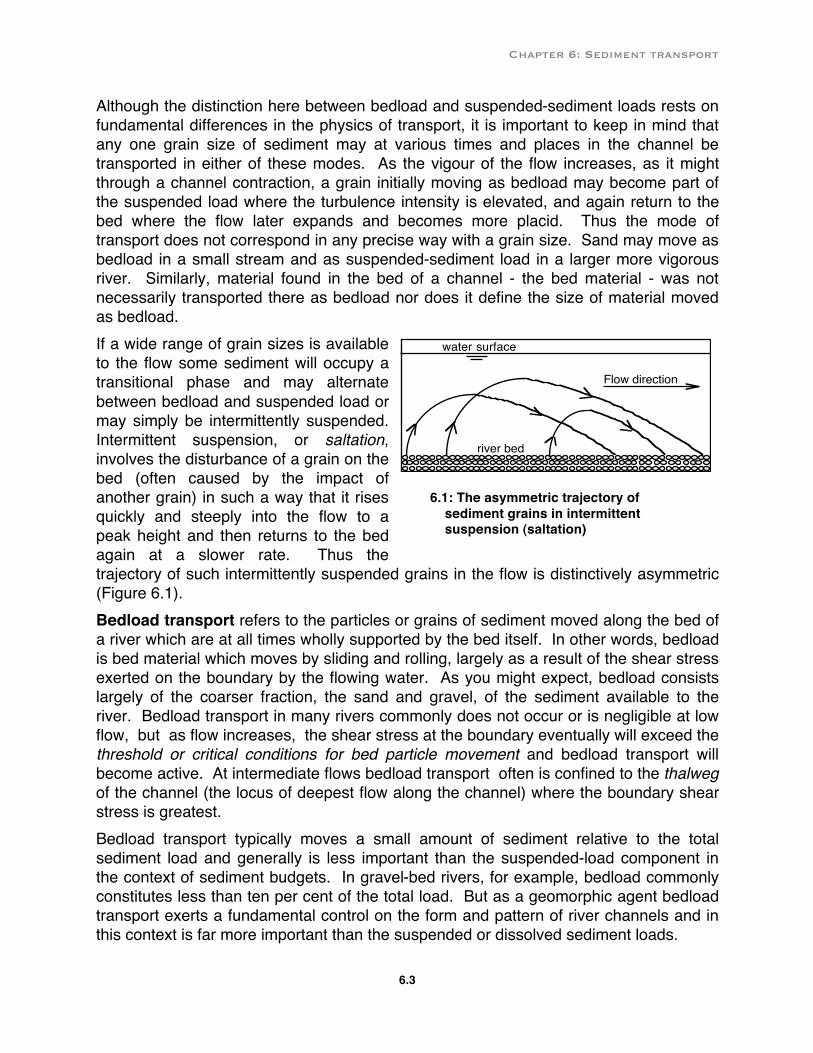
Although the distinction here between bedload and suspended-sediment loads rests on fundamental differences in the physics of transport, it is important to keep in mind that any one grain size of sediment may at various times and places in the channel be transported in either of these modes. As the vigour of the flow increases, as it might through a channel contraction, a grain initially moving as bedload may become part of the suspended load where the turbulence intensity is elevated, and again return to the bed where the flow later expands and becomes more placid. Thus the mode of transport does not correspond in any precise way with a grain size. Sand may move as bedload in a small stream and as suspended-sediment load in a larger more vigorous river. Similarly, material found in the bed of a channel - the bed material - was not necessarily transported there as bedload nor does it define the size of material moved as bedload. If a wide range of grain sizes is available to the flow some sediment will occupy a transitional phase and may alternate between bedload and suspended load or may simply be intermittently suspended. Intermittent suspension, or saltation, involves the disturbance of a grain on the bed (often caused by the impact of another grain) in such a way that it rises quickly and steeply into the flow to a peak height and then returns to the bed again at a slower rate. Thus the trajectory of such intermittently suspended grains in the flow is distinctively asymmetric (Figure 6.1). Bedload transport refers to the particles or grains of sediment moved along the bed of a river which are at all times wholly supported by the bed itself. In other words, bedload is bed material which moves by sliding and rolling, largely as a result of the shear stress exerted on the boundary by the flowing water. As you might expect, bedload consists largely of the coarser fraction, the sand and gravel, of the sediment available to the river. Bedload transport in many rivers commonly does not occur or is negligible at low flow, but as flow increases, the shear stress at the boundary eventually will exceed the threshold or critical conditions for bed particle movement and bedload transport will become active. At intermediate flows bedload transport often is confined to the thalweg of the channel (the locus of deepest flow along the channel) where the boundary shear stress is greatest. Bedload transport typically moves a small amount of sediment relative to the total sediment load and generally is less important than the suspended-load component in the context of sediment budgets. In gravel-bed rivers, for example, bedload commonly constitutes less than ten per cent of the total load. But as a geomorphic agent bedload transport exerts a fundamental control on the form and pattern of river channels and in this context is far more important than the suspended or dissolved sediment loads.

6.1: The asymmetric trajectory of sediment grains in intermittent suspension (saltation)

water surface

Flow direction

river bed


6.4

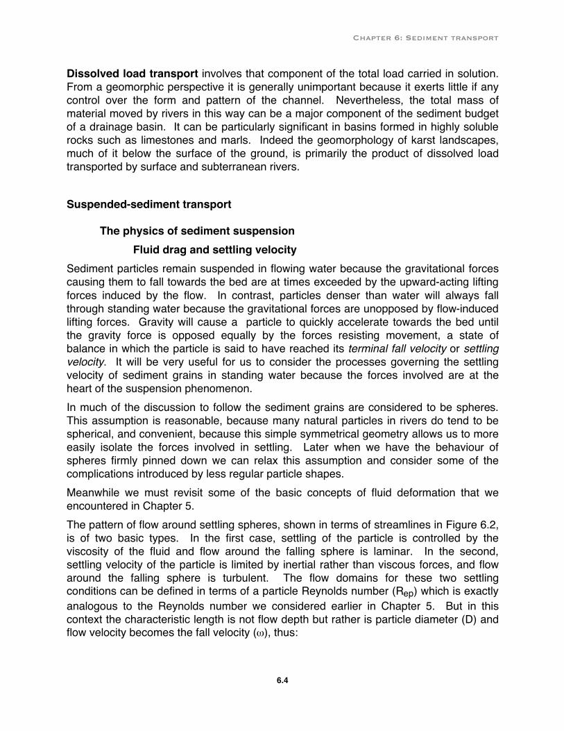
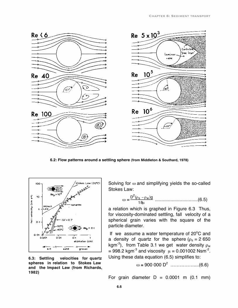
Dissolved load transport involves that component of the total load carried in solution. From a geomorphic perspective it is generally unimportant because it exerts little if any control over the form and pattern of the channel. Nevertheless, the total mass of material moved by rivers in this way can be a major component of the sediment budget of a drainage basin. It can be particularly significant in basins formed in highly soluble rocks such as limestones and marls. Indeed the geomorphology of karst landscapes, much of it below the surface of the ground, is primarily the product of dissolved load transported by surface and subterranean rivers. Suspended-sediment transport The physics of sediment suspension Fluid drag and settling velocity Sediment particles remain suspended in flowing water because the gravitational forces causing them to fall towards the bed are at times exceeded by the upward-acting lifting forces induced by the flow. In contrast, particles denser than water will always fall through standing water because the gravitational forces are unopposed by flow-induced lifting forces. Gravity will cause a particle to quickly accelerate towards the bed until the gravity force is opposed equally by the forces resisting movement, a state of balance in which the particle is said to have reached its terminal fall velocity or settling velocity. It will be very useful for us to consider the processes governing the settling velocity of sediment grains in standing water because the forces involved are at the heart of the suspension phenomenon. In much of the discussion to follow the sediment grains are considered to be spheres. This assumption is reasonable, because many natural particles in rivers do tend to be spherical, and convenient, because this simple symmetrical geometry allows us to more easily isolate the forces involved in settling. Later when we have the behaviour of spheres firmly pinned down we can relax this assumption and consider some of the complications introduced by less regular particle shapes. Meanwhile we must revisit some of the basic concepts of fluid deformation that we encountered in Chapter 5. The pattern of flow around settling spheres, shown in terms of streamlines in Figure 6.2, is of two basic types. In the first case, settling of the particle is controlled by the viscosity of the fluid and flow around the falling sphere is laminar. In the second, settling velocity of the particle is limited by inertial rather than viscous forces, and flow around the falling sphere is turbulent. The flow domains for these two settling conditions can be defined in terms of a particle Reynolds number (Rep) which is exactly analogous to the Reynolds number we considered earlier in Chapter 5. But in this context the characteristic length is not flow depth but rather is particle diameter (D) and flow velocity becomes the fall velocity (ω), thus:


6.5

Rep = inertial forcesviscous forces = ωD

ν.....................................(6.2)

When Rep < 0.1 grain settling is constrained overwhelmingly by viscous resistance. This condition is met only when the grains are small (in the silt-clay range; D<0.0625 mm diameter) so that inertial effects are negligible and the grain falls sufficiently slowly that laminar flow occurs throughout and the streamline pattern is symmetrical about the vertical axial streamline which meets and leaves the sphere at two stagnation points where velocity is zero (Figure 6.2). At these stagnation points shear stress is also zero but, as implied by the Bernoulli equation, surface pressure at these points must be at a maximum; a typical pattern of shear stress and pressure around a sphere falling at low particle Reynolds number is depicted in Figure 6.2. The resistance to flow encountered by an object moving through a fluid is known as the drag force (FD) and is the sum of all forces opposing the movement. Physical reasoning suggests that, in this case of a sphere falling in a viscosity-dominated low Reynolds number environment, the drag force will depend simply on the size of the sphere, the fluid viscosity, and the settling velocity. Dimensional analysis yields (see Chapter 1) the general relation: FD = kµDω ...........................................................(6.3) in which the constant k can be shown by experiment to be equal to 3π. In fact, the British physicist Sir George Stokes (1819-1903) working early last century demonstrated analytically that the k = 3π so that the particular form of equation (6.3) can be taken as: FD = 3πµDω .........................................................(6.4) We can now derive an expression for the settling velocity (which is constant and therefore implies zero net force acting on the sphere) under these circumstances by equating the impelling force - the submerged weight of the sphere - to the drag force in equation (6.4). The impelling force for a sphere is specified by Fg = ma where the mass is the product of the sphere volume ( 1

6πD3), the buoyancy-discounted density (ρs-ρw)

and a is gravitational acceleration (g). Thus we can state that, since Fg = FD,

1 6πD3(ρs-ρw)g = 3πµDω


6.6

6.2: Flow patterns around a settling sphere (from Middleton & Southard, 1978)

Solving for ω and simplifying yields the so-called Stokes Law:

ω =D2(ρs −ρw)g18µ .................................(6.5)

a relation which is graphed in Figure 6.3 Thus, for viscosity-dominated settling, fall velocity of a spherical grain varies with the square of the particle diameter. If we assume a water temperature of 20oC and a density of quartz for the sphere (ρs = 2 650 kgm-3), from Table 3.1 we get water density ρw = 998.2 kgm-3 and viscosity µ = 0.001002 Nsm-2. Using these data equation (6.5) simplifies to: ω ≅ 900 000 D2 ……………....(6.6)

For grain diameter D = 0.0001 m (0.1 mm)

6.3: Settling velocities for quartz spheres in relation to Stokes Law and the Impact Law (from Richards, 1982)


6.7

equation (6.6) predicts a fall velocity ω = 0.009 ms-1 (0.9 cms-1), a result consistent with experiment (see Figure 6.3). For a grain diameter D = 0.01 m (1.0 cm), however, equation (6.6) predicts a fall velocity ω = 90.0 ms-1 (9000 cms-1), absurdly higher than experience indicates is reasonable. Clearly, Stokes Law is beyond its domain in this large grain-size range. An application of Stokes law is illustrated in Sample Problem 6.1.

Sample Problem 6.1:

Problem : A quartz silt particle (D50 =0.05 mm) is carried in suspension by a stream which flows into a 58 m-deep lake where it settles to the bottom. If the freshwater lake has a temperature of10oC, calculate the length of time required for the sediment particle to settle from the lake surface to the bottom.

Solution: We need to determine the settling velocity from Stokes law ω =D2 (ρs − ρw )g

18µ

. We know

from Table 2.1 that µ= 1.307x10-3 Nsm-2, ρs=2650 kgm-3 and ρw =1000 kgm-3. Given g = 9.806 ms-2 and

D= 5x10-5 m, Stokes law yields: ω =(5x10−5)2(2650 − 1000)9.806

18(1.307x10−3 )= 1.719x10−3ms−1 . The settling time, t, is

therefore t = 581.719x10−3

= 33741s . In other words, in the absence of interfering currents, the particle

would take about 9 hrs to settle to the bottom of the lake. The reason for the failure of Stokes Law to predict accurately the fall velocity of grains in excess of about 0.1 mm diameter is illustrated in Figure 6.2. As grain size increases above this value the inertial forces become so great that the now negligible viscous forces are no longer able to constrain the settling behaviour of the particle. The particle Reynolds number for these conditions increases to values many orders of magnitude greater than one. This corresponds to the flow around the sphere becoming fully turbulent and separating from the leeward side creating a separation bubble or wake behind the particle as it falls. Within the wake zone the highly sheared flow at the separation boundary drives a complex pattern of eddying. In certain circumstances instability along the line of separation can result in margins of the wake being folded into the flow (wake shedding) and eddies can be ejected in a remarkably periodic fashion forming a so-called von Karman vortex street. Fluid pressure within the wake is much lower than that at the leading surface of the sphere and this “suction” behind the sphere acts to retard the fall velocity. The importance of eliminating this low-pressure wake zone in many practical applications such as aircraft and automobile design is recognized in the process of “streamlining”, leading to cigar-shaped forms which fill the potential lee-side separation bubble and thereby reduces the overall resistance to flow (drag). Obviously we need to take a different approach to specifying the governing equation for fall velocity under these higher Reynolds number flows where inertia of the water is the dominating resisting force. Following Rubey (1933) we can change our frame of reference and conceptualize the constant fall-velocity behaviour as one in which the


6.8

spherical grain is held stationary in the flow by the impact of a rising column of water. An impact force, equal to the rate of momentum transfer per unit time from the water to the sphere is provided by the rising cylindrical column of water which has a cross-sectional area equal to the projected area of the falling sphere ( π4 D

2 ). In unit time the

water-column mass is the product of the volume ( π4 D2ω) and fluid density (ρw) and

momentum is the product of the water mass and the fall velocity (ω) so we can say that the ʻimpact forceʼ (FI) is given by: FI = π4 D

2ρwω2 ......................................................(6.7)

For a constant fall velocity we can equate FI and the submerged weight of the sphere [Fg= 1

6πD3(ρs-ρw)g] to give:

1 6πD3(ρs-ρw)g = π4 D

2ρwω2

Solving for ω and simplifying yields the Impact Law:

ω = 23Dg(ρs − ρw)

ρw .....................................(6.8)

Again, for the conditions specified above to develop equation (6.6), equation (6.8) similarly can be simplified to give: ω = 3.3 D ..................................................(6.9) For example, a grain size D = 0.01 m (1.0 cm), equation (6.9) predicts a fall velocity ω = 0.33 ms-1 (33.0 cms-1), a value consistent with observation (see Figure 6.3). At the intersection of Stokes and the Impact Laws there is a transitional phase corresponding to the sand-size range (0.06-2 mm) in which viscous and inertial effects are both important. Here a composite law applies (derived by balancing Fg with the sum of Fd and Fi; see Rubey, 1933):

1 6πD3(ρs-ρw)g = 3πµDω + π4 D

2ρwω2

or D2(ρs-ρw)g = 18µω + 32Dρwω2...........................................(6.10)

and is graphed in Figure 6.3 (equation (6.10) is a quadratic but easily solved numerically; see Appendix 1.1).


6.9

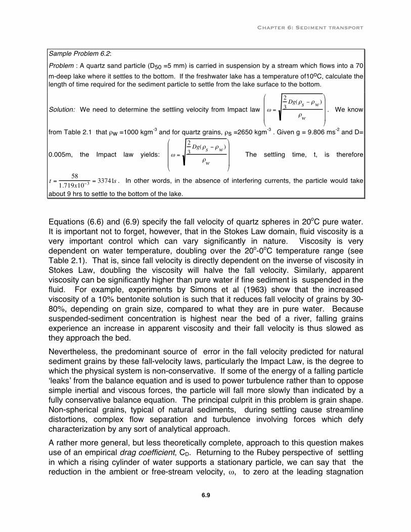
Sample Problem 6.2:

Problem : A quartz sand particle (D50 =5 mm) is carried in suspension by a stream which flows into a 70 m-deep lake where it settles to the bottom. If the freshwater lake has a temperature of10oC, calculate the length of time required for the sediment particle to settle from the lake surface to the bottom.

Solution: We need to determine the settling velocity from Impact law ω =

23Dg(ρs − ρw )

ρw

. We know

from Table 2.1 that ρw =1000 kgm-3 and for quartz grains, ρs =2650 kgm-3 . Given g = 9.806 ms-2 and D=

0.005m, the Impact law yields: ω =

23Dg(ρs − ρw )

ρw

The settling time, t, is therefore

t =58

1.719x10−3= 33741s . In other words, in the absence of interfering currents, the particle would take

about 9 hrs to settle to the bottom of the lake.

Equations (6.6) and (6.9) specify the fall velocity of quartz spheres in 20oC pure water. It is important not to forget, however, that in the Stokes Law domain, fluid viscosity is a very important control which can vary significantly in nature. Viscosity is very dependent on water temperature, doubling over the 20o-0oC temperature range (see Table 2.1). That is, since fall velocity is directly dependent on the inverse of viscosity in Stokes Law, doubling the viscosity will halve the fall velocity. Similarly, apparent viscosity can be significantly higher than pure water if fine sediment is suspended in the fluid. For example, experiments by Simons et al (1963) show that the increased viscosity of a 10% bentonite solution is such that it reduces fall velocity of grains by 30-80%, depending on grain size, compared to what they are in pure water. Because suspended-sediment concentration is highest near the bed of a river, falling grains experience an increase in apparent viscosity and their fall velocity is thus slowed as they approach the bed. Nevertheless, the predominant source of error in the fall velocity predicted for natural sediment grains by these fall-velocity laws, particularly the Impact Law, is the degree to which the physical system is non-conservative. If some of the energy of a falling particle ʻleaksʼ from the balance equation and is used to power turbulence rather than to oppose simple inertial and viscous forces, the particle will fall more slowly than indicated by a fully conservative balance equation. The principal culprit in this problem is grain shape. Non-spherical grains, typical of natural sediments, during settling cause streamline distortions, complex flow separation and turbulence involving forces which defy characterization by any sort of analytical approach. A rather more general, but less theoretically complete, approach to this question makes use of an empirical drag coefficient, CD. Returning to the Rubey perspective of settling in which a rising cylinder of water supports a stationary particle, we can say that the reduction in the ambient or free-stream velocity, ω, to zero at the leading stagnation


6.10

point on any particle involves a loss of kinetic energy (KE= mω2

2 ). Again, in unit time, m = Aωρw so that KE= Aωρwω2

2 =ρwω

3A2 ....................................................(6.11)

where A is the projected area of the particle. Energy and work are interchangeable concepts and Equation (6.11) also can be interpreted as specifying the rate of doing work, or power, P =W

t . Also, by definition, W = Fs (force x distance), and st = ω , so in this case of a settling particle, P = FDω (where FD is the drag force acting on the grain) leading to: FDω =

ρwω3A

2

or FD = ρwω2A

2 .......................................................(6.12)

In recognition of the effect of particle shape on FD, a drag coefficient, CD, is introduced in equation (6.12) so that

FD= CDρwω

2A2 ......................................................(6.13)

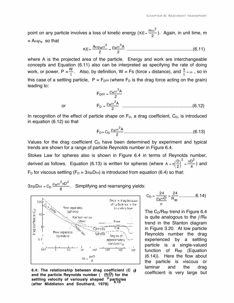
Values for the drag coefficient CD have been determined by experiment and typical trends are shown for a range of particle Reynolds number in Figure 6.4. Stokes Law for spheres also is shown in Figure 6.4 in terms of Reynolds number, derived as follows. Equation (6.13) is written for spheres (where A = π

D2

2

=πD2

4 ) and

FD for viscous settling (FD = 3πµDω) is introduced from equation (6.4) so that: 3πµDω = CD

ρwω2πD2

8 . Simplifying and rearranging yields:

CD =24

ρwωDµ

=24Rep

.............6.14)

The CD/Rep trend in Figure 6.4 is quite analogous to the ƒ/Re trend in the Stanton diagram in Figure 3.20. At low particle Reynolds number the drag experienced by a settling particle is a single-valued function of Rep (Equation (6.14)). Here the flow about the particle is viscous or laminar and the drag coefficient is very large but 6.4: The relationship between drag coefficient (C )

and the particle Reynolds number ( ) for the settling velocity of variously shaped particles (after Middleton and Southard, 1978)

Dρu Dµ


6.11

declines by an order of magnitude (from CD ≅ 100 to 10) in the range 0.1<Rep<1.0. As Reynolds number increases above Rep ≅ 1.0, the drag continues to decline but at a rate less than that predicted by Stokes Law. For cylinders flow separation begins at about Rep = 6. In this phase, leeside eddying, vortex shedding and general turbulence begin to markedly influence particle drag. For the domain in which Rep>100, drag coefficients change little with increasing values of Reynolds number. Here flow around the settling particle is fully turbulent and drag is essentially independent of the viscous forces and therefore the Reynolds number. In this zone of Rep-independent drag coefficients, variations in CD occur only in response to changes in particle shape; highly streamlined bodies have low drag coefficients in the region of 0.1, roughly spherical bodies have values of about 0.5 and extremely blunt objects, such as a disk oriented normal to the flow, may have drag coefficients as high as 1.0 or more. Fall velocities of markedly non-spherical particles, particularly platy or disklike objects, may be even lower than their drag coefficients suggest because of instability in their settling motion. For example, photographic studies (Stringham et al, 1969) show that, while disks fall with a steady and flat attitude at low particle Reynolds number, as Rep increases the falling particle develops a regular lateral oscillation (like a slowly falling leaf), then an inclined gliding motion eventually coupled with tumbling. The particle fall trajectory can involve a significant lateral component and the vertical fall velocity is distinctly less than is the velocity along the trajectory actually followed. Oscillatory behaviour of this sort associated with the strongly periodic stresses involved in eddy shedding behind blunt objects in turbulent flow are common. Everyday examples of this effect are revealed in the humming of wires and cables in the wind and the vibration of partly submerged tree limbs in flowing rivers. All these complications relating to fall velocity have led sedimentologists to think in terms of the true diameter of a particle (the measured b-axis length) and the effective diameter (or equivalent, apparent, sedimentation or hydraulic diameter ) of a particle (the diameter of a same-density sphere with the same fall velocity), on the other. It is reasoned that particles with the same sedimentation diameter (fall velocity) are subject to the same kind of transport and sedimentation behaviour regardless of the true particle diameter. The diffusion model of sediment suspension As we noted earlier, sediment grains are suspended in the flow above the bed when the vertical component of turbulence equals their fall velocity. Actually, it has been argued (see Bagnold, 1956) that, even in isotropic turbulence (in which turbulence scales and intensity are uniform throughout the flow), and therefore where the strength of the upward velocity component is the same as the downward component, suspension can be maintained. In this case of isotropic turbulence it is envisaged that some grains will diffuse away from the region of high concentration near the bed by the grain collisions and ʻnear missesʼ which together give rise to a poorly understood net upward force termed the intergranular dispersive stress. It would appear that some such mechanism must be at work since it has been shown that, even in laminar flow, grains can be dispersed from near the bed to higher positions in the flow (Francis, 1973).


6.12

In conditions of isotropic turbulence the downward (or negative direction) movement of grains from a point in the flow where there is a grain concentration C of uniformly sized grains, is described by: rate of settling per unit volume of fluid = -ωC ..........................(6.15) If we assume that the upward vertical movement of particles is a diffusion process like many others in which the diffusion rate is proportional to the concentration gradient (Fickʼs Law), we can also say that:

rate of turbulent diffusion per unit volume = εsdCdy

.......................(6.16)

Equating equations (6.15) and (6.16) gives an equation describing the vertical distribution of the concentration of suspended particles:

ωC + esdCdy

= 0 ...............................................(6.17)

The diffusion coefficient, εs, should be constant for any given field of isotropic turbulence and we might expect it to be directly related to the corresponding diffusion coefficient for fluid momentum (ie, the eddy viscosity, ε; see equation 5.12), an expectation that has been confirmed experimentally (Rouse, 1939). Of course, in rivers we are dealing with shear flows where we have anything but isotropic turbulence and the key to developing the idea of equation (6.17) for this case is to specify how εs varies in the y direction above the bed.

Assuming the direct proportionality, εs= βε (and so ε = εsβ

), and recalling equation

(5.8), τ = ερ dvdy , we can say that:

τ =εsρβ

dvdy

..............................................(6.18)

where β is a coefficient probably close to unity.

Recalling equation (4.5), we can say that τo = γds, where τo = boundary shear stress and d = the total depth of flow. Within uniform flow the shear stress at any height y above the bed is a linear function of the depth of overlying water so that τ = γ(d-y)s, from which it follows (by dividing τ = γ(d-y)s by τo = γds) that:

τ = τo 1−

yd

....................................(6.19)

Combining equations (6.18) and (6.19) yields:

εsρβ

dvdy

=τo 1− yd


6.13

which can be rearranged to give εs =

βτoρ

1− yd

dvdy

............................….............(6.20)

Recalling that shear velocity, V* = τoρ

, and introducing from equation (5.14) the “law of

the wall” ( dvdy =V*

Ky ), equation (6.20) becomes

εs = βV* 1− yd

Ky .................................................(6.21)

Equation (6.21) describes how εs varies with height y above the bed and provides the process link needed to solve equation (6.17). Combining these yields:

ωC + βV* 1− yd

Ky dC

dy

= 0

which can be rearranged to give dCC =−ω dy

βKV* 1− yd

y

...........……………………..........(6.22)

Integrating equation (6.22) yields:

lnC =ω

βKV*dy

1− yd

ya

d

∫

or CCa

=d − yy

ad − a

z

where z = ω

βKV* ......……...(6.23)

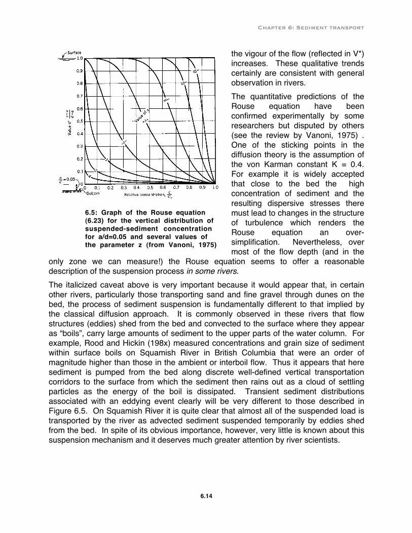
Equation (6.23) is known as the Rouse equation and the exponent z as the Rouse Number, after Professor Hunter Rouse, the pioneering American hydraulic engineer who first derived the equation in 1937. The Rouse equation gives the concentration of sediment, C, of a given settling velocity, ω, at height y above the bed, relative to the concentration at height a above the bed; the graph of this equation is shown in Figure 6.5. Thus, equation (6.23) does not predict an absolute suspended-sediment concentration but describes the vertical distribution given some known concentration Ca at height y = a (usually obtained as close to the bed as possible). This classical treatment of sediment suspension outlined above is consistent with general observation. Other things constant, as the settling velocity (and Rouse Number decreases) the vertical distribution of sediment changes from being markedly concentrated near the bed (at z >1.0) to quite uniform with respect to depth (at z < 132 ).

Similarly, for sediment of a given settling velocity we see the same trend produced as


6.14

the vigour of the flow (reflected in V*) increases. These qualitative trends certainly are consistent with general observation in rivers. The quantitative predictions of the Rouse equation have been confirmed experimentally by some researchers but disputed by others (see the review by Vanoni, 1975) . One of the sticking points in the diffusion theory is the assumption of the von Karman constant K = 0.4. For example it is widely accepted that close to the bed the high concentration of sediment and the resulting dispersive stresses there must lead to changes in the structure of turbulence which renders the Rouse equation an over-simplification. Nevertheless, over most of the flow depth (and in the

only zone we can measure!) the Rouse equation seems to offer a reasonable description of the suspension process in some rivers. The italicized caveat above is very important because it would appear that, in certain other rivers, particularly those transporting sand and fine gravel through dunes on the bed, the process of sediment suspension is fundamentally different to that implied by the classical diffusion approach. It is commonly observed in these rivers that flow structures (eddies) shed from the bed and convected to the surface where they appear as “boils”, carry large amounts of sediment to the upper parts of the water column. For example, Rood and Hickin (198x) measured concentrations and grain size of sediment within surface boils on Squamish River in British Columbia that were an order of magnitude higher than those in the ambient or interboil flow. Thus it appears that here sediment is pumped from the bed along discrete well-defined vertical transportation corridors to the surface from which the sediment then rains out as a cloud of settling particles as the energy of the boil is dissipated. Transient sediment distributions associated with an eddying event clearly will be very different to those described in Figure 6.5. On Squamish River it is quite clear that almost all of the suspended load is transported by the river as advected sediment suspended temporarily by eddies shed from the bed. In spite of its obvious importance, however, very little is known about this suspension mechanism and it deserves much greater attention by river scientists.

6.5: Graph of the Rouse equation (6.23) for the vertical distribution of suspended-sediment concentration for a/d=0.05 and several values of the parameter z (from Vanoni, 1975)


6.15

Direct measurement of suspended-sediment transport rate

Because no complete theory of suspended-sediment transport is available, measurement of suspended-sediment concentrations are critical to specifying the rate of transport. Bedload Transport The physics of bed material transport The physics of bed material movement involves two fundamental, and in many ways independent, processes: sediment entrainment and transport maintenance. Of these two sets of processes the first is by far the more complicated to analyze and invariably is the problem at the root of any failure to accurately predict bedload transport rates in rivers. Whether or not entrainment occurs depends on the ratio of entraining to resisting forces: Ce = entraining forces

resisting forces .....................................................(6.24)

If the coefficient Ce = 1.0 in equation (6.1) the grain at rest on the bed is said to be at the threshold of motion. Ce < 1.0 implies no motion and Ce >1.0 is the state of entrainment. Similarly, once a particle has become entrained in the flow, whether or not transport is maintained depends on the ratio of transporting forces to resisting forces:

Ct = transporting forcesresisting forces ....................................................(6.25)

Provided Ct in equation (6.1) remains at or above unity, the particle will remain in motion. Although equations (6.1) and (6.2) are conceptually identical they are operationally quite different because the entraining forces are not the same as the transporting forces (since the former is for a grain at rest and the latter is for one in motion) nor are the resisting forces identical in the two cases. For example, a grain may form part of an imbricated gravel bed, locked in place by neighbouring particles. In order to entrain the grain, sufficient force must be brought to bear on several particles in order to dislodge the grain from its resting place; less force is required to overcome the resisting forces once the grain is in motion. This circumstance is quite analogous to an aircraft which must expend greater energy (apply greater force) to overcome ground and air friction in order to become airborne than it does to overcome just air friction in order to stay aloft. Sediment entrainment, as noted above, occurs just beyond the threshold of motion at Ce = 1.0, when the entraining forces = resisting forces. Both sets of forces are very


6.16

complex, however, and the condition for the threshold defies analysis in all but the simplest cases. Nevertheless, it will be instructive to consider the forces involved qualitatively and to consider an analytical solution which at least illustrates the nature of the problem and provides the basis for some widely used semi-empirical models for defining the conditions for incipient motion . The entraining forces involve at least three groups of applied forces: • impact force • shear stress (drag force) • lift forces (buoyancy, hydrodynamic lift, turbulence)

The impact force is the result of direct momentum transfer to the grain as the water impacts on the upstream-projected surface area. Actually, we have considered already the nature of the impact force in the context of the discussion of fall velocity. The impact force, Fi, for a single spherical grain at rest on a plane bed, is given by equation (6.3) if ω is replaced by the ambient velocity, v, striking the sphere: Fi = ρwv2

π4

D2 ..............................................................(6.26)

That is, the impact force is proportional to the flow velocity and grain diameter squared. Of course, equation (6.26) has no practical utility and its actual use would have to incorporate an empirical coefficient (ϑ ) to at least allow for the effects of grain sheltering (degree of exposure to the oncoming flow), grain shape, and the fact that not all of the force of the directly impinging water is expended on the sphere (Fi = ϕρwv2D2 ).

Shear stress is the tangential force exerted by the fluid as it flows over and around the grain on the bed. The unit force exerted on the sphere as the water shears over the channel boundary is given directly by equation (4.5). In a channel of rectangular cross-section the total shear stress applied to a single spherical particle on the bed (sometimes termed the tractive force) is given by the product of the shear stress term in equation (4.5) and the surface area of the sphere, thus:

τo = ρwgdsϕπD2

4 .........................................................(6.27)

where, again, ϕ is a coefficient reflecting the degree to which the sphere surface is exposed. Of course, if the shear stress were not uniformly distributed across the channel, a shear stress term such as that based on the local velocity distribution would be more appropriate than the depth/slope product (see Problem 5.3). The lift forces include the buoyant force, the hydrodynamic lift force, and the upward turbulence flux. The buoyant force is the hydrostatic force resulting from the particle/fluid density differences and is easily accounted for in the usual way as the buoyancy-discounted or submerged weight of the particle. The hydrodynamic lift force occurs because a grain on the bed is in the zone of steepest velocity gradient and the velocity at the base of the grain is considerably less than that at the top. In accordance with Bernoulli (which specifies an inverse relationship between velocity and pressure),


6.17

there is an upward declining pressure gradient which tends to lift the grain off the bed. The role of turbulence is not independent of the pressure-gradient force because excursions of velocity above the mean flow velocity obviously intensify that gradient temporarily and increase the lift at those times. But turbulence also involves other lifting forces, mostly not well understood. As water shears over the bed, turbulence is generated at the boundary in the form of wakes consisting of spinning parcels of water or vortices (eddies). These vortices move from the bed up into the flow, providing irregular upward pulses or bursts of high-velocity fluid motion. The upward force applied to bed particles by turbulence probably is the most important component of the lift force. Unfortunately it is also exceedingly complex and not amenable to any realistic analytical treatment. It is also very difficult to measure although several notable experimental studies (reviewed in Vanoni, 1975), suggest that the lift force can equal the drag force and exceed it by a factor of two or more in some flume flows. It has been argued that, because the lift forces involve the same basic variables as the drag force, the general expressions for both forces will have the same structure; see equation (6.12). The general lift equation for a spherical bed particle, therefore, becomes: FL = CLk2D

2ρwvo22 ..............................................(6.28)

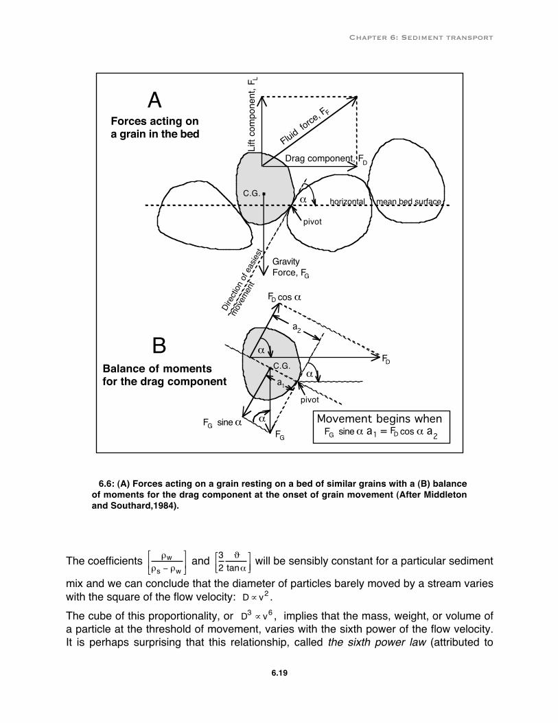
where CL is a lift coefficient (analogous to the drag coefficient), k2 is a particle shape factor, and Vo is flow velocity at the level of the particle. We might note that this relation only applies to fully turbulent flows (viscosity is omitted from consideration). This constraint is hardly limiting, however, since the viscous sublayer in all natural river flows would be completely disrupted by turbulence near the boundary. The relations among these competing forces is summarized in Figure 6.6A which shows a force diagram for roughly spherical particles resting on a river bed. Because the downstream slope of most channels is very small compared with the angle of repose of the grains in the bed we can assume that the mean bed surface is horizontal. The submerged weight or gravity force acts vertically downward through the centre of gravity of the grain and it is also subjected to the resultant of a horizontal drag force (or alternatively, an impact force) and a vertical lift force. Most analytical treatments of entraining forces acting on a grain on the bed consider only drag; lift does not appear explicitly. But it is argued that, because the resulting theoretical equations include coefficients of proportionality which are determined experimentally, and because lift depends on the same variables as drag, the effect of lift is automatically incorporated into the solutions. This may not seem like compelling reasoning to everyone but an alternative approach has yet to be offered and the assumption certainly is convenient and leads to some interesting and useful results. For example, if the incipient motion of the particle shown in Figure 6.6 involves rolling or rotating about a pivot point in the surface of easiest movement, the gravity and drag


6.18

forces can be resolved in that direction and the moments of the opposing forces can be equated to define the condition of incipient motion (see Figure 6.6B) as: FG sin α a1 = FD cos α a2 .............................................(6.29) where a1 and a2 are the unequal turning arms. The horizontal drag force FD in equation (6.29) is easily replaced by a more comprehensive resultant of both the lift forces and the drag force or by an alternative force such as the impact force. We will consider a couple of simple approaches but as we shall soon see, these analytical solutions have quite significant limitations and it is more useful to resort to a more general approach to the problem of defining incipient motion. It is not surprising that early thinking about incipient motion was in terms of flow velocity. The connection seemed so obvious that other factors influencing sediment motion were long neglected. We can derive an expression for incipient motion by solving equation (6.29) where the drag force is replaced by the impact force from equation (6.26) generalized to particles of projected area A (Fi = ρwv2A ). The gravity force exerted by a grain of volume, VO , is given by FG = Vo(ρs − ρw)g.

Thus, we can say that, at the point of incipient motion, the balance of moments is:

Vo(ρs −ρw)gsineαa1 = ρwv2Aϑcosαa2

which can be simplified to VoA =ρw

ρs − ρw

ϑtanα

a2a1

v2

g ..........................………......(6.30)

in which ϑ is a coefficient of grain exposure. In the case of spheres, for which the turning arms a1 and a2 are equal, Vo =

16 πD

3 and projected A =π4D

2 , equation (6.30)

simplifies further to

D =ρw

ρs − ρw

32

ϑtanα

v2

g ........................................(6.31)


6.19

Fluid force

, FF

Drag component, FD

Lift

com

pone

nt, F

LGravityForce, FG

horizontal mean bed surfaceC.G.

pivot

α

AForces acting on a grain in the bed

BBalance of moments for the drag component

C.G.

pivot

α

α

FG

F sineG α

a1

αFD

FD cos α

a2

Dire

ction

of e

asies

t

movem

ent

FD cos αF sineG α a1a = 2

Movement begins when

6.6: (A) Forces acting on a grain resting on a bed of similar grains with a (B) balance of moments for the drag component at the onset of grain movement (After Middleton and Southard,1984).

The coefficients ρwρs − ρw

and 3

2ϑ

tanα

will be sensibly constant for a particular sediment

mix and we can conclude that the diameter of particles barely moved by a stream varies with the square of the flow velocity: D∝ v2 . The cube of this proportionality, or D3 ∝ v6 , implies that the mass, weight, or volume of a particle at the threshold of movement, varies with the sixth power of the flow velocity. It is perhaps surprising that this relationship, called the sixth power law (attributed to


6.20

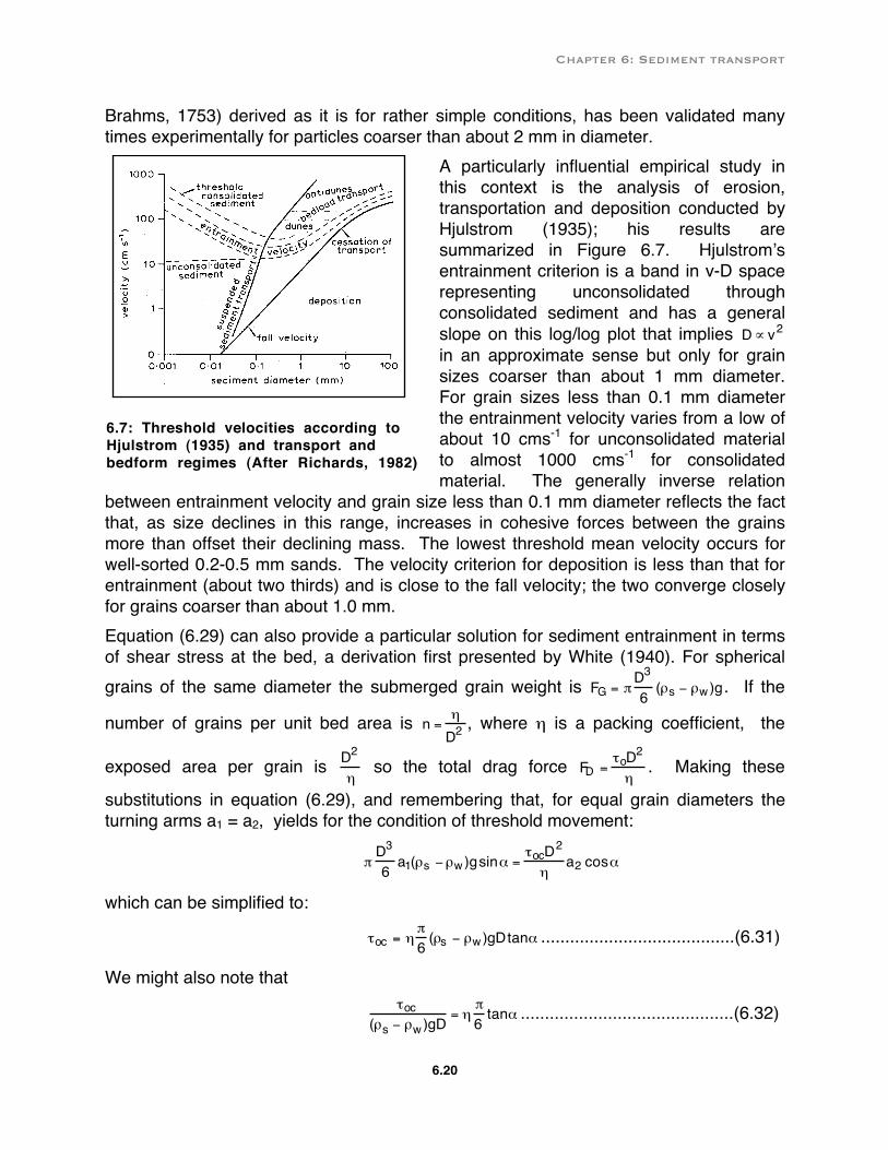
Brahms, 1753) derived as it is for rather simple conditions, has been validated many times experimentally for particles coarser than about 2 mm in diameter.

A particularly influential empirical study in this context is the analysis of erosion, transportation and deposition conducted by Hjulstrom (1935); his results are summarized in Figure 6.7. Hjulstromʼs entrainment criterion is a band in v-D space representing unconsolidated through consolidated sediment and has a general slope on this log/log plot that implies D∝ v2 in an approximate sense but only for grain sizes coarser than about 1 mm diameter. For grain sizes less than 0.1 mm diameter the entrainment velocity varies from a low of about 10 cms-1 for unconsolidated material to almost 1000 cms-1 for consolidated material. The generally inverse relation

between entrainment velocity and grain size less than 0.1 mm diameter reflects the fact that, as size declines in this range, increases in cohesive forces between the grains more than offset their declining mass. The lowest threshold mean velocity occurs for well-sorted 0.2-0.5 mm sands. The velocity criterion for deposition is less than that for entrainment (about two thirds) and is close to the fall velocity; the two converge closely for grains coarser than about 1.0 mm. Equation (6.29) can also provide a particular solution for sediment entrainment in terms of shear stress at the bed, a derivation first presented by White (1940). For spherical grains of the same diameter the submerged grain weight is FG = π

D3

6 (ρs − ρw)g. If the

number of grains per unit bed area is n = η

D2, where η is a packing coefficient, the

exposed area per grain is D2

η so the total drag force FD =

τoD2

η. Making these

substitutions in equation (6.29), and remembering that, for equal grain diameters the turning arms a1 = a2, yields for the condition of threshold movement:

π D3

6 a1(ρs −ρw)gsinα =τocD2

ηa2 cosα

which can be simplified to:

τoc = ηπ6 (ρs − ρw)gDtanα ........................................(6.31)

We might also note that

τoc(ρs − ρw)gD

= ηπ6 tanα ............................................(6.32)

6.7: Threshold velocities according to Hjulstrom (1935) and transport and bedform regimes (After Richards, 1982)


6.21

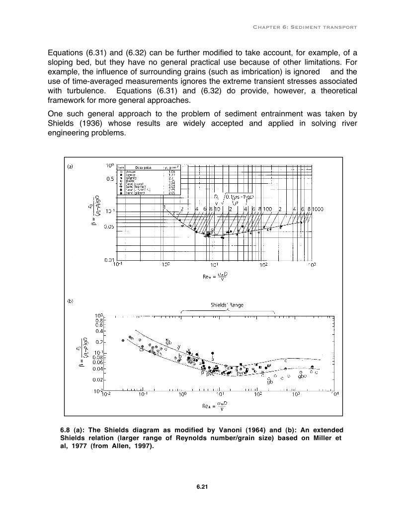
Equations (6.31) and (6.32) can be further modified to take account, for example, of a sloping bed, but they have no general practical use because of other limitations. For example, the influence of surrounding grains (such as imbrication) is ignored and the use of time-averaged measurements ignores the extreme transient stresses associated with turbulence. Equations (6.31) and (6.32) do provide, however, a theoretical framework for more general approaches. One such general approach to the problem of sediment entrainment was taken by Shields (1936) whose results are widely accepted and applied in solving river engineering problems.

6.8 (a): The Shields diagram as modified by Vanoni (1964) and (b): An extended Shields relation (larger range of Reynolds number/grain size) based on Miller et al, 1977 (from Allen, 1997).


6.22

Shields used experimental data to characterize, for a range of particle Reynolds number, the behaviour of the equilibrium force balance in a dimensionless critical shear stress term called the Shields criterion:

θc =τoc

(ρs − ρw)gD....................................................(6.33)

The structural similarity of equations (6.33) and (6.32) is quite apparent and reveals the physical basis of the Shields entrainment function which is graphed in Figure 6.8. For small Reynolds number (Rep<1.0) Shields dimensionless shear stress is high but declines to a minimum at about Rep ≅ 10. This domain of the Shields entrainment function corresponds with the silt/clay grain size range and the high values of θc are thought to reflect the fact that the grains are protected by the enclosing laminar sublayer as well as being bound strongly one to another by strong electrochemical forces among the grains. As Reynolds number increases to Rep ≅ 10 the grains emerge from the thinning laminar sublayer into the turbulent flow and the increasing grain size into the coarse silt and sand range is associated with weakening moved of all particle sizes and θc reaches a minimum approaching 0.03. As Rep increases from 10 to 500 through the sand sizes into the gravel fraction, Shields dimensionless shear stress increases from about 0.03 to a plateau value of 0.06 for all higher values of Rep in fully turbulent flow over gravel. The asymptote at θc = 0.06 is particularly significant because it allows a useful simplification of equation (6.33) for use in estimating the critical shear stress for particle motion in gravel-bed rivers: If θc =

τoc(ρs − ρw)gD

= 0.06,

τoc = 0.06(ρs − ρw)gD.............................................(6.34)

For quartz particles in pure water equation (6.34) simplifies further to τoc ≈ 970D............................................................(6.35)

There is considerable scatter in the empirical data used to define the Shields entrainment function and it is prudent to allow for a range of θc where equation (6.34) represents the minimum shear stress required for motion. A suggestion offered by Church (19xx) in this regard is to vary θc between 0.05 and 0.07 in accordance with the packing state of particles in the bed. If the sediment-transporting flow declines abruptly, as it might do after a flash flood, the bed particles do not have an opportunity to mutually adjust, one to the other, and the bed packing is minimal; the bed packing state here is said to be overloose. At the other extreme, prolonged flows near the point of incipient motion can promote imbrication and the development of gravel structures which correspond with an underloose packing state. Most channel beds have packing states between these end member conditions and are described as having a normal packing state for which θc = 0.06.


6.23

Measuring bedload transport rate To be continued ……………………….


6.24

6.1: The asymmetric trajectory of sediment grains in intermittent suspension (saltation) 6.2: Flow patterns around settling spheres at low (laminar flow) and high (turbulent flow) Reynolds numbers (L or M&S) 6.3: Settling velocities for quartz spheres in relation to Stokes Law and the Impact Law (KR) 6.4: Drag coefficient and Reynolds number (M&S) 6.5: Plot of Rouse equation (ASCE, 77) 6.6: (A) Forces acting on a grain resting on a bed of similar grains with a (B) balance of moments for the drag component at the onset of grain movement (After Middleton and Southard,1984). 6.7: Hjulstrom curve 6.8: Shields Function


6.25

Measuring bedload transport rate Formulae for predicting bedload-transport rate Bedforms Character Origins Role in sediment transport Total load measurements Sediment sources and sediment supply Drainage basin characteristics Supply-limited sediment transport The geography of sediment discharge from rivers


6.26

Documents

Sediment transport - SFU.cahickin/FLUIDS/Chapt6-Sediment transport.pdf · Direct measurement of suspended-sediment transport rate ... The geography of sediment discharge from rivers