Sensitivity Analysis of Surface Runoff Generation for

11th

International Conference on Urban Drainage, Edinburgh, Scotland, UK, 2008

Adeyemo et al. 1

Sensitivity Analysis of Surface Runoff Generation for Pluvial

Urban Flooding

O.J. Adeyemo1*, C. Maksimovic

1, S. Booyan-Aronnet

1, J. Leitao

1, D. Butler

2, C.

Makropoulos2

1Urban Water Research Group, Department of Civil and Environmental Engineering, Imperial College London,

London SW7 2AZ, UK. 2Centre for Water Systems, University of Exeter, Exeter EX4 4QF, UK *Corresponding author, e-mail [email protected]

ABSTRACT

Significant advances have been made in recent times in the domain of integrated hydraulic

modelling of urban flooding. Development of a physically based model for dual drainage

concept, in which urban surface is treated as a network of open channels and ponds (major

system) connected to the sewer network (minor system), has been a step forward (Boonya-

aroonnet et al. 2006). However, generation of reasonably realistic surface network is the main

concern in this methodology (Djordjevic et al. 2005).

This paper presents the results obtained by new developed tools (Boonya-aroonnet et al.

2007) for enhancing the potential of 1D/1D modelling by more accurate GIS-based automatic

generation of surface network features. The application of these tools to a real life case study

is discussed.

Simplification of high resolution of LiDAR Digital Terrain Model (DTM) by re-sampling

original 1x1m grid to larger sizes is necessary and sensitivity is analysed. Number of ponds

removed and cumulative and discrete volume loss charts were generated and used to

determine the suitable threshold values for removal of small ponds.

In generating the pathways cross-section geometry, multi-criteria optimization technique was

deployed to study the sensitivity of the input parameters on the geometries generated and

appropriate parameter selection process.

KEYWORDS Pluvial urban flooding, sensitivity analysis, dual drainage, surface flow network

INTRODUCTION

The flood problems arising from urban flooding range from minor ones, such as water

entering the basements of a few houses, to major incidents, where large parts of cities are

inundated for several days. Most modern cities in the industrialized world have been facing

small-scale local problems mainly due to insufficient capacity in their sewer systems during

heavy rainstorms (Mark et al. 2004). Hence, prevention of flooding in urban areas caused by

inadequate sewer systems has become an important issue. With increased property values of

buildings and other structures, potential damage from prolonged flooding can easily become

economically catastrophic. For instance, in the UK, during July 2007, floods have damaged

nearly 30,000 homes and 7,000 businesses and have taken the lives of some people as well.

Insurers think the clean-up bill will top 2 billion pounds1. The service fees paid by residents

are used to operate and maintain urban drainage systems effectively without fear of failure,

thereby keeping the level of service acceptable. However, drainage systems are designed to

cope with a defined project storm, i.e. if a stronger storm happens, flood problems may occur.

1 http://en.wikipedia.org/wiki/2007_United_Kingdom_floods

11th


Adeyemo et al. 2

Thus, in establishing tolerable flood frequencies, the safety of the residents and the protection

of their valuables must be in balance with the technical and economic restrictions (Schmitt et

al 2004).

The Urban Water Research Group (UWRG) of Imperial College London have been engaged

in research to enhance the potential of 1D/1D type of model by more accurate GIS-based

automatic generation of surface flow characteristics such as ponds and flow pathways, cross-

section geometry, connectivity, area-depth curves within the AUDACIOUS2 and FRMRC

3

projects. The approach is based on Digital Elevation Model (DEM) and land-use images

derived from high resolution and accuracy acquisition techniques. The work presented here is

a contribution to the ongoing research at the group. It covers the preparation of input data and

detailed investigation into the sensitivity analysis of the parameters associated with the

developed tool. Simulations of the dual drainage system were carried out using InfoWorks,

taking into account the surface flow network generated with the developed tool.

Figure 1 presents the overall process described in this paper. The main objectives are:

1. Investigate some of the sensitivity issues associated with the GIS based tool as

reported by Boonya-aroonnet et al. (2007). This has to do with the sensitivity of the

various parameters to be used in developing the appropriate overland model;

2. Using appropriate parameters based on the investigation, develop the surface network

model using the GIS-Based tool. The surface pathway network for the model consists

of storage nodes (with its characteristics) and links (with its shapes);

3. Introduce the output of the surface network model into commercial software,

InfoWorks;

4. Simulate a 1D-1D (i.e. one-dimensional in both surface network and sewer pipe flow)

urban pluvial flooding applying the dual drainage concept model in InfoWorks;

5. Investigate the potentials of the use of the GIS based tool in planning new

developments especially with respect to pluvial urban flooding;

6. Identify areas for further research

METHODOLOGY TO GENERATE SURFACE FLOW NETWORK AND SIMULATE

URBAN PLUVIAL FLOOD

Data Preparation

LiDAR data, in ESRI ASCII Grid format, was obtained from the Environment Agency. Data

resolution is 1x1m and went through a classification and filtering processes in order to

produce Digital Terrain Models (DTM) from the original Digital Surface Model (DSM).

Using ArcGIS®

Desktop 9.1, IDRISI®

Andes and CatchmentSIM®

, the necessary project files

to generate the overland flow network modelling phase of the project were created, including

slope and aspect images.

Two sets of DTMs were prepared – original and smooth. Smoothening was done to remove

spurious depressions and flat areas and as many problematic features as possible. About 10

iterations of the filling algorithm in CatchmentSim®

were applied to the original DTMs to

produce the smooth ones.

The original 1m resolution data from LiDAR was resampled to produce DTMs with the

following cell sizes: 2x2m, 4x4m, 5x5m, 8x8m and 10x10m. This exercise was carried out

for both the original and smooth data sets.

2 Adaptable Urban Drainage – Addressing Change in Intensity, Occurrence and Uncertainty of

Stormwater 3 Flood Risk Management Research Consortium

11th


Adeyemo et al. 3

Elvetham Heath

Case Study

- LiDAR DATA

Data

Preparation

Input DataSurface Flow

Network Analysis

Pond

Delineation

Pathway

Delineation

Generate Cross

Section

Geometry

Dual Drainage

Simulation

Inputs

Data Preparation

into Infoworks

format

Network Capacity

Analysis

Infoworks Simulation:

Dual Drainage System

(under extreme events)Proposed

Sewer Network

System

SENSITIVITY

ANALYSIS

SENSITIVITY

ANALYSIS

Figure 1 Overview of the Application of the GIS-Based Tool in a Case Study

Sensitivity Analysis

The sensitivity analysis was carried out on some vital input parameters of the GIS-based

routines in order to determine the appropriate value parameters to obtain the best

representation of overland flow. Specifically, these are the pond filtering parameters of pond

delineation procedure and the parameters to generate flow pathways cross sections.

The sensitivity analysis at the pond delineation phase was carried out on all the datasets

prepared, both original and smoothened. After this stage and following an analysis of the

result, a DTM was chosen. Flow pathways were created using only the chosen DTM.

Sensitivity analysis at the Cross Section Geometry process was conducted using the adopted

DTM.

The objective of the exercise at the pond delineation module was to determine the threshold

value of depth and volume parameters that ensure elimination of noise from the DTM while

minimising volume loss. Combinations of volume variations of 1m3, 2m

3, 3m

3, 4m

3 and 5m

3

were employed with depth variations of 0.004m, 0.008m, 0.01m, 0.02m, 0.03m, 0.04m,

0.06m, 0.08m, 1.0m, 1.5m and 2.0m.

The objective of the exercise at the cross-section module was to determine the appropriate

combination of the parameters such that there are a minimal number of cross sections ending

up with the user pre-defined sections.

11th


Adeyemo et al. 4

Case Study - Location and General Overview

The case study used for this project is Elvetham Heath. Elvetham Heath is an ongoing 1,868-

home development in the prospering suburbs of Hampshire (UK). It is located immediately to

the north of Fleet in the borough of Hart. It is bounded to the North by the M3 motorway and

the Fleet motorway service area and to the South by the London/Southampton railway line.

To the East is the North Hampshire Golf Club and to the West the A323. It is connected by a

40 – 80 minute train service from central London and is located 5-minute drive from the

nearby town of Fleet (Figure 2).

Figure 2. Location of Elvetham Heath Fleet

The predominant land use is residential occupying 0.63km2 of the 1.26km

2 site. Sewer system

has approximately 62 manholes over the sewered area of the analysis.

RESULTS AND DISCUSSION

Pond Delineation

Without applying any filtering parameters, the number of ponds generated in the original

DTM data sets range from 607 to 32,766 while that of the smoothened DTM data sets range

from 137 to 3,561. A summary of the result obtained for the smoothened DTM data sets is

shown in Table 1

Table 1 – Normalized Volume and Pond Loss for Smooth DTMs without applying any filter

parameter

Cell Size No of Ponds Volume of Ponds

(m) (No) (m3)

1x1 7,303 116,158

2x2 1,865 113,995

4x4 749 105,270

5x5 501 99,961

8x8 189 94,543

10x10 137 90,516

Figure 3 shows the normalised plots showing the relationship between DTM cell size, pond

loss and volume loss. From the results obtained, it can be deduced that the shift from 1x1m

DTM to a 2x2m DTM, which resulted in a loss of 90% of the ponds but only 9% of the total

volume, may have led to a significant reduction in noise/pit cells in the further analysis of the

DTM. Thereafter, it was observed that an almost linear relationship exists between the pond

loss and volume loss for the DTM with cell sizes 4x4m, 5x5m, 8x8m, and 10x10m. This may

represent a more physical volume loss commensurate with the corresponding pond loss.

11th


Adeyemo et al. 5

0.00

0.25

0.50

0.75

1.00

1x1 2x2 4x4 5x5 8x8 10x10

DEM Cell Size

No

rm

alize

d P

on

ds

0.00

0.25

0.50

0.75

1.00

No

rm

alize

d V

olu

me

Pond Loss

Vol Loss

Figure 3. Normalized Volume and Pond Loss for Smoothened DTMs without applying any

filter parameter

The filtering was done to remove the ponds that satisfy both depth and volume criteria but the

DTM remain unchanged. Though due to the limitation in the capacity of the tool, the volume

figures for the original 1x1m DTM could not be determined, similar trend was observed in the

results obtained from simulations with the original DTMs.

Based on these observations, the 2x2m DTM was adopted for further detailed analysis.

Figure 4 shows the spatial distribution of the ponds for the 2x2m DTM cell size and this gives

a physical appreciation of the ponds, which helps to analyse the potential of flood

vulnerability in the area. The choice of the 2x2m DTM is consistent with the

recommendations of a cell size of between 1x1m and 5x5m DTM resolution for urban flood

analysis (Mark et al 2004).

Pond Filtering

This analysis was carried out for all the datasets. Thus, volume-loss curves such as those in

Figure 5 were generated. From the curves generated, three zones were identified, Zones A, B

and C. In Zone A, the five volumes being tested against various depths exhibits the same

trend. This may be due to the very small depth values being tested in relation to cell sizes. It

is also believed that some noise is still inherent in the DTM in this zone.

In Zone B, the individual volume loss curves spread out further, reflecting their relative

volume values. From each curve, there is a point where further variation in depth does not

produce any change in the cumulative volume loss. This point is here referred to as the Pond

Filtering Optimum Depth (PFOD). And Zone C is the zone after the PFOD for each volume

curve. It was also observed that the coarser the DTM being tested, the more pronounced is

Zone C as the PFOD is attained quicker.

Lisbon Data Set

To determine whether the curves and trends observed on the cumulative volume-loss charts

for the Elvetham Heath data sets can be standardised for the GIS-based routine tool, the

analysis was further conducted on a dataset from Lisbon (Portugal). The source of the Lisbon

DTM is also LiDAR, originally in 1x1m resolution and then re-sampled to different cell sizes

– 2x2m, 4x4m, 5x5m, 8x8m, and 10x10m.

11th


Adeyemo et al. 6

Figure 4. Spatial Distribution of Ponds Generated in 2x2m DTM resolution (Elvetham)

Figure 5. Cumulative Volume Loss Curve for a 2x2m DTM

From the curves generated with the Lisbon datasets, the three zones were also observed, but

their lengths and sizes differ. For instance, Zone A is more pronounced in the Lisbon data

sets and PFOD is hardly attained with the depths tested. This may be due to the fact that the

results from the use of this tool will reflect to a large extent, terrain characteristics, which is

different from place to place.

Threshold Values for Pond Filtering

From the cumulative volume-loss charts, it can be clearly determined, for each volume filter

value, the PFOD, which is the point at which further increases in depths will not longer result

in any further reduction in cumulative volume. However, further analysis was necessary to

determine the combination of volume / depth threshold value. This was carried out bearing in

mind the major goals of this exercise, which is to achieve a balance between minimisation of

volume loss and elimination of noise from the DTM.

Zone A

Zone B

Zone C

PFOD

11th


Adeyemo et al. 7

The approach adopted to carry out this analysis was to plot the differential (discrete) volume

loss curves against the depth values. The result of this is as shown in Figure 6. The depth

0.02m came out as the turning point for the pond curves. On the volume curves, the turning

point (depth value) for the 1m3 line coincide with the value from the ponds’ curves and a

linear increase was observed for the turning points from 1m3 to 5m

3.

(a) (b)

Figure 6 (a,b) Differential (Discrete) changes in ponds/volume vs depths

From this, 0.02m was adopted as the threshold depth value for the 2x2m DTM. This is the

inflexion point in differential ponds’ curves, which also correspond to the lowest inflexion

point on the differential volume curves. The threshold volume adopted was 1m3. Here, the

volume loss is 0.112% of the total pond volume; the surface area of the ponds filtered is

473,040m2, which represents about 14.60% of the total area of the catchment.

Figure 7 shows the pond distributions for the 2x2m-filtered DTM in terms of volume and

surface areas.

88

427

198

44 47 9 12 0 1 10

200

400

600

800

1000

1200

1 10 50 100 500 1000 10000 20000 30000 40000

Vol (cub m)

Fre

quency

0 0

192146

400

48 22 19

0

100

200

300

400

500

600

700

800

1 10 50 100 1000 2500 5000 40000

Vol (sq m)

Fre

qu

en

cy

(a) Ponds’ Volume Distribution – 2x2m

DTM (Filtered)

(b) Ponds’ Area Distribution – 2x2m DTM

(Filtered)

Figure 7. 2x2m Smoothened DTM pond volume and area distribution before and after

filtration

Flow pathways delineation

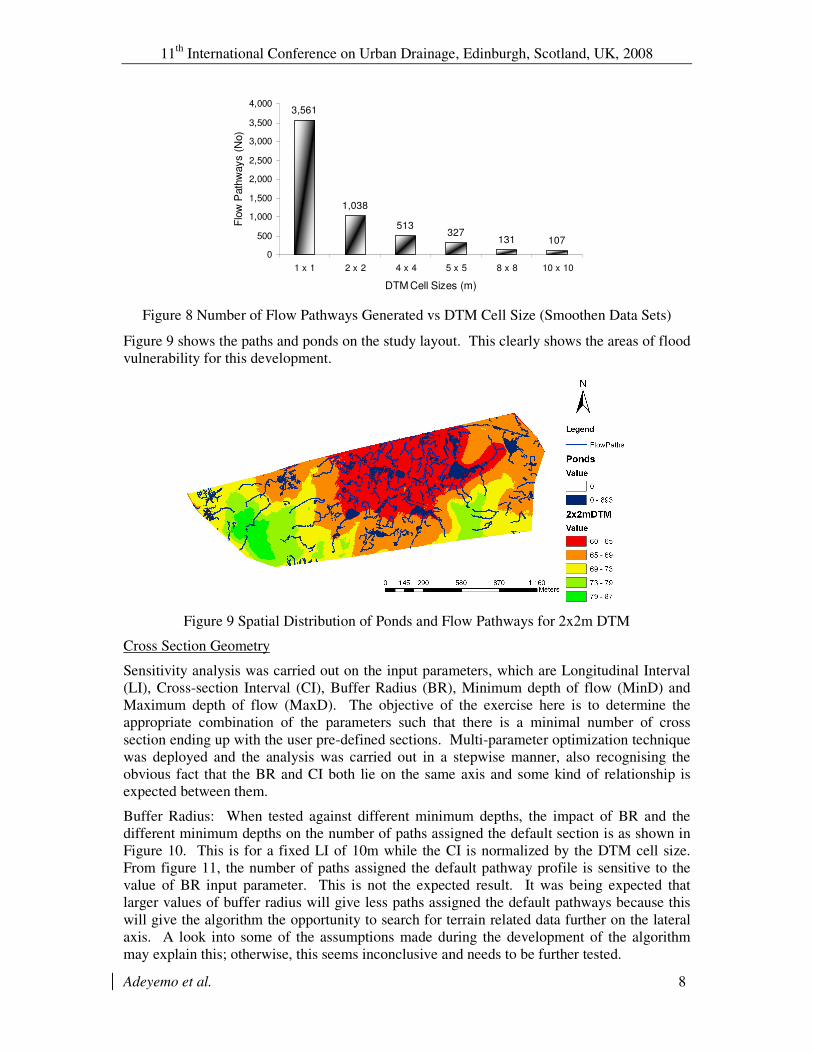
Figure 8 shows the number of pathways generated for different DTM cell sizes, without

applying any filter parameters to the DTMs. The path delineation exercise for the 2x2m DTM

with the selected filter parameters eventually resulted in the generation of 519 flow pathways

connecting the ponds together.

11th


Adeyemo et al. 8

3,561

1,038

513327

131 107

0

500

1,000

1,500

2,000

2,500

3,000

3,500

4,000

1 x 1 2 x 2 4 x 4 5 x 5 8 x 8 10 x 10

DTM Cell Sizes (m)

Flo

w P

ath

ways (

No)

Figure 8 Number of Flow Pathways Generated vs DTM Cell Size (Smoothen Data Sets)

Figure 9 shows the paths and ponds on the study layout. This clearly shows the areas of flood

vulnerability for this development.

Figure 9 Spatial Distribution of Ponds and Flow Pathways for 2x2m DTM

Cross Section Geometry

Sensitivity analysis was carried out on the input parameters, which are Longitudinal Interval

(LI), Cross-section Interval (CI), Buffer Radius (BR), Minimum depth of flow (MinD) and

Maximum depth of flow (MaxD). The objective of the exercise here is to determine the

appropriate combination of the parameters such that there is a minimal number of cross

section ending up with the user pre-defined sections. Multi-parameter optimization technique

was deployed and the analysis was carried out in a stepwise manner, also recognising the

obvious fact that the BR and CI both lie on the same axis and some kind of relationship is

expected between them.

Buffer Radius: When tested against different minimum depths, the impact of BR and the

different minimum depths on the number of paths assigned the default section is as shown in

Figure 10. This is for a fixed LI of 10m while the CI is normalized by the DTM cell size.

From figure 11, the number of paths assigned the default pathway profile is sensitive to the

value of BR input parameter. This is not the expected result. It was being expected that

larger values of buffer radius will give less paths assigned the default pathways because this

will give the algorithm the opportunity to search for terrain related data further on the lateral

axis. A look into some of the assumptions made during the development of the algorithm

may explain this; otherwise, this seems inconclusive and needs to be further tested.

11th


Adeyemo et al. 9

LI = 10m; MinD = 0.01m

0

10

20

30

40

50

60

70

0 2 4 6 8 10

Normalized (CI/Cell Size)

Path

s w

ith d

efa

ult S

ection A

ssig

ned

(%)

BR=10m

BR=15m

BR=20m

BR=25m

BR=30m

LI = 10m; MinD = 0.05m

0

10

20

30

40

50

60

70

0 2 4 6 8 10


Path

s w

ith d

efa

ult

Sectio

n A

ssig

ned (

%)

BR=10m

BR=15m

BR=20m

BR=25m

BR=30m

(a) Minimum depth of 0.01m (b) Minimum depth of 0.05m

Figure 10 – Buffer Radius Sensitivity Curves for different Minimum Depths

Cross-sectional Interval: From Figures 10, it can be deduced that the number of paths

assigned the default pathway profile is also sensitive to the value of the cross-section interval

used for the analysis. For a given BR, the higher the CI, the lower the number of pathways

assigned the default sections. Also, at a CI value of 8 times the cell size, the BR values tested

gave the same result. Also, based on the findings, the cross sectional interval must be chosen

such that it is less than or equal to the buffer radius (CI < BR).

Minimum Depth: As shown in Fig 10 (a) and (b), the number of paths assigned the default

pathway profile are sensitive to the Minimum depth value used for the analysis. With a given

LI of 10m, it was observed that the range of the output values for various BRs with a MinD of

0.01m is 18-60%. For a MinD of 0.05m, this range is 30-65%.

Longitudinal Interval: Figure 11 (a-b) suggests that the number of paths assigned the default

pathway profile is not sensitive to the value of LI. In physical terms, this will appear untrue

because the shorter the distances between the cross-sections, the more details are captured to

give a representation of the channel cross-section, which is close to reality. A value of 4

times the cell size also seems to be an optimum CI for this data set.

Maximum Depth: The maximum depth of flow was found not to be a sensitive parameter.

However, a value of 1m is however recommended.

LI = 10m; MinD = 0.01m

0

10

20

30

40

50

60

70

0 2 4 6 8 10


Path

s w

ith d

efa

ult S

ection A

ssig

ned

(%)

BR=10m

BR=15m

BR=20m

BR=25m

BR=30m

LI = 20m; MinD = 0.01m

0

10

20

30

40

50

60

70

0 2 4 6 8 10


Path

s w

ith d

efa

ult S

ection A

ssig

ned (

%)

BR=10m

BR=15m

BR=20m

BR=25m

BR=30m

(a) Sensitivity of BR: LI=10m, MinD=0.01m (b) Sensitivity of BR: LI=20m, MinD=0.01m

Figure 11 Sensitivity of Longitudinal Interval and Cross-section Interval

Summary

Based on the analysis done and the application of judgement, the following values were

adopted - Longitudinal Interval – 10m; Maximum Depth – 2m; Minimum Depth – 0.01m;

Cross Section Interval – 6x cell size; Buffer Radius – 20m. With these parameters, 37% of

the 519 flow pathways identified were assigned the default pathway.

11th


Adeyemo et al. 10

CONCLUSIONS

The GIS-based tool is indeed an innovation and its completion and deployment has the

potential to assist in the identification of areas prone to pluvial flooding. This would be very

useful to modellers and planners, especially when analysing such issues such as system

performance and effects caused by new urban developments under extreme rainfall events.

The main conclusions of the sensitivity analysis research carried out in this project are as

follows:

1. The DTM size adopted for analysis will affect the modelling results. There is the need

to choose the right DTM cell size for analysis when using this tool.

2. Pond delineation/filtering – When filtering ponds to eliminate noise while minimising

volume loss, the combination of pond depth and volume is a sensitive filtering

parameter.

3. From the comparison between the results obtained from testing Elvetham and Lisbon

data sets, it was clear that the Volume Loss Curves’ characteristics are not

standardised for different data sets. Hence, there is the need to develop appropriate

charts for new datasets to be modelled with the tool.

4. Cross Section Geometry: Based on the sensitivity analysis carried out on the input

parameters to generate the appropriate cross-section geometry, the following

conclusions are drawn:

a. The number of pathways generated representing the terrain features is sensitive

to the input parameters of Cross-section interval (CI), minimum depth of open

channels and Buffer radius. Different combinations of these are possible. The

following recommendations are based on the results and analysis from this

study – a value of CI between 6 and 8 times the DTM cell size and a Min

Depth of 0.01m.

b. Maximum Depth is not sensitive – a value greater than or equal to 1m is

recommended.

c. Longitudinal Interval (LI) was expected to be an important parameter, which

should have been sensitive, but it appears not to be sensitive. There is the need

to investigate further into this issue.

d. Though the Buffer Radius turns out to be a sensitive parameter as expected but

it exhibits a somewhat ‘reversed’ sensitivity. There is a need for further

investigation into this as well.

REFERENCES

Boonya-aroonnet, S., Maksimović, Č, Prodanović, D. & Djordjević, S. 2007, "Urban Pluvial

Flooding: Development of GIS based Pathways Model for Surface Flooding and Interface

with Surcharged Sewer Model", Proceedings of NOVATECH 2007, pp. 481.

Boonya-aroonnet, S., Prodanović, D. & Maksimović, Č 2006, "Advance Overland Flow

Modelling for Urban Pluvial Flood Analysis", Proc of the 14th Congress of SAHR(ex-IAHR).

Djordjevic, S., Prodanovic, D., Maksimovic, C., Ivetic, M. & Savic, D. 2005, SIPSON -

Simulation of interaction between pipe flow and surface overland flow in networks, IWA

Publishing, Alliance House 12 Caxton Street London SW1H 0QS UK.

Mark, O., Weesakul, S., Apirumanekul, C., Aroonnet, S.B. & Djordjevic, S. 2004, "Potential

and limitations of 1D modelling of urban flooding", Journal of Hydrology (Amsterdam), vol.

299, no. 3-4, pp. 284-299.

Schmitt, T.G., Thomas, M. & Ettrich, N. 2004, "Analysis and Modelling of Flooding in Urban

Drainage Systems", Journal of Hydrology, vol. 299, pp. 300-311.

Documents

Sensitivity Analysis of Surface Runoff Generation for