Sensitivity of Model-Based EpidemiologicalParameter Estimation to Model Assumptions

A.L. Lloyd

Abstract Estimation of epidemiological parameters from disease outbreak dataoften proceeds by fitting a mathematical model to the data set. The resulting param-eter estimates are subject to uncertainty that arises from errors (noise) in the data;standard statistical techniques can be used to estimate the magnitude of this uncer-tainty. The estimates are also dependent on the structure of the model used in thefitting process and so any uncertainty regarding this structure leads to additionaluncertainty in the parameter estimates. We argue that if we lack detailed knowledgeof the biology of the transmission process, parameter estimation should be accom-panied by a structural sensitivity analysis, in addition to the standard statisticaluncertainty analysis. Here we focus on the estimation of the basic reproductive num-ber from the initial growth rate of an outbreak as this is a setting in which parameterestimation can be surprisingly sensitive to details of the time course of infection.

1 Introduction

Estimation of epidemiological parameters, such as the average duration of infec-tiousness or the basic reproductive number of an infection, is often an importanttask when examining disease outbreak data [see, for example, 12, 19, 26]. In manyinstances, one or more parameters of interest cannot be estimated directly from theavailable data, so an indirect approach is adopted in which a mathematical modelof the transmission process is formulated and is fitted to the data. The resultingparameter estimates will have uncertainty due to noise in the data but they will alsodepend on the form chosen for the model. Any uncertainties in our knowledge of thebiology underlying the transmission process lead to uncertainties in the parameterestimates over and above those that arise from noise in the data.

Standard statistical approaches (see Chapters 1, 5, 7, 10 and 11 of this book) canbe used to quantify the uncertainty in parameter estimates that arises from noise in

A.L. Lloyd (B)Biomathematics Graduate Program and Department of Mathematics, North Carolina StateUniversity, Raleigh, NC 27695, USAe-mail: alun lloyd@ncsu.edu

G. Chowell et al. (eds.), Mathematical and Statistical Estimation Approachesin Epidemiology, DOI 10.1007/978-90-481-2313-1 6,C© Springer Science+Business Media B.V. 2009

123

124 A.L. Lloyd

the data, but these are not designed to provide insight into the sensitivity of the esti-mates to the structure of the model. In this chapter, we demonstrate that uncertaintydue to model structure can, in some instances, dwarf noise-related uncertainty bydiscussing an estimation problem in which details of the description of the biologyof the transmission process can have an important impact. This argues that whenthere is incomplete knowledge of the biology of the infection, structural sensitiv-ity analysis should accompany statistical uncertainty analysis when model-basedapproaches are used to interpret epidemiological data.

In this chapter, we illustrate the potential importance of model assumptionsby examining the model-based estimation of the basic reproductive number usingdata obtained from the initial stages of a disease outbreak. We review studies[21, 25, 27, 31, 33, 34] that illustrate that such estimates can be highly sensitiveto the assumptions made concerning the natural history of the infection, particularlyregarding the timing of secondary transmission events. These results are of majorsignificance in the setting of emerging infectious disease outbreaks, when a rapidquantification of the basic reproductive number is highly desirable to guide controlefforts, but when information on the transmission cycle may be scarce. Importantly,the work shows that the use of simple models can greatly underestimate the valueof the basic reproductive number, providing overly optimistic predictions for howeffective control measures have to be in order to curtail the spread of the disease.

2 The Basic Reproductive Number and Its EstimationUsing the Simple SIR Model

The basic reproductive number, R0, is defined as the average number of secondaryinfections caused by a typical infective individual in an otherwise entirely sus-ceptible population [see, for example, 11]. In the simplest settings, its value canbe calculated as the product of the rate at which such an individual gives rise toinfections and the duration of their infectious period. In turn, the infection rate isa product of the rate at which an infective meets susceptible individuals, i.e. thecontact rate, and the per-contact probability of transmission.

Direct estimation of the basic reproductive number could be undertaken if sec-ondary infections of individual infectives could be quantified. Unfortunately, themost commonly available type of data—aggregated incidence data—does not revealtransmission chains in sufficient detail to identify the source of secondary cases.More detailed data, such as contact tracing data, can elucidate chains of transmis-sion, but is rarely complete enough to allow direct calculation of R0. In the absenceof complete contact tracing data, statistical techniques have been suggested for theestimation of R0 via reconstruction of transmission chains [13, 32].

The basic reproductive number could also be directly estimated if both the con-tact rate and transmission probability were known. Again, direct estimation ofthese quantities is typically difficult. Transmission probabilities can be estimatedusing certain types of epidemiological data, obtained, for instance, from observation

Sensitivity of Model-Based Epidemiological Parameter Estimation 125

of transmission within families, or other transmission experiments. Such data,however, are often unavailable during the early stages of a disease outbreak.

An alternative approach involves fitting a mathematical model to outbreak data,obtaining estimates for the parameters of the model, allowing R0 to be calculated.The simplest model that can be used for this purpose is the standard deterministiccompartmental SIR model [see, for example, 11]. Individuals are assumed to eitherbe susceptible, infectious or removed, with the numbers of each being written asS, I , and R, respectively. Susceptible individuals acquire infection through con-tacts with infectious individuals, and the simplest form of the model assumes thatnew infections arise at rate βSI/N . Here N is the population size and β is thetransmission parameter, which is given by the product of the contact rate and thetransmission probability. Recovery of infectives is assumed to occur at a constantrate γ , corresponding to an average duration of infection of 1/γ , and leads to per-manent immunity. Throughout this chapter we shall denote the average duration ofinfectiousness by DI and assume permanent immunity following infection. We shallalso ignore demographic processes (births and deaths), which is a good approxi-mation if the disease outbreak is short-lived and the infection is non-fatal. Ignoringdemography leads to the population size N being constant. The model can be writtenas the following set of differential equations

dS/dt = −βSI/N (1)

dI/dt = βSI/N − γ I (2)

dR/dt = γ I. (3)

During the early stages of an outbreak with a novel pathogen, almost the entirepopulation will be susceptible, and, since S ≈ N , the transmission rate equalsβ I . The transmission parameter β is the rate at which each infective gives riseto secondary infections and so the basic reproductive number can be written asR0 = βDI = β/γ . During this initial period, the changing prevalence of infec-tion can, to a very good approximation, be described by the single linear equationd I/dt = γ (R0 − 1)I. (We remark that the S = N assumption corresponds tolinearizing the model about its infection free equilibrium.) In other words, providedthat R0 is greater than one, which we shall assume to be the case throughout thischapter, prevalence initially increases exponentially with growth rate

r = γ (R0 − 1). (4)

The incidence of infection is given by βSI/N and so, during the early stages ofan outbreak, prevalence and incidence are proportional in the SIR setting, so thisequation also describes the rate at which incidence grows.

Equation (4) provides a relationship, R0 = 1 + r DI, between R0 and quan-tities that can typically be measured (the initial growth rate of the epidemic andthe average duration of infection), and as a result has provided one of the moststraightforward ways to estimate R0.

126 A.L. Lloyd

3 More Complex Compartmental Models

The SIR model of Section 2 employs a very simple, but quite unrealistic, descrip-tion of the time course of infection. The infectious period is assumed to startimmediately upon infection, and the constant recovery rate corresponds to infec-tious periods being exponentially distributed across the population. In reality, thereis a delay—the latent period—between acquisition of infection and the start ofinfectiousness: an individual typically receives a small dose of an infectious agentand several rounds of replication have to occur within the infected person beforethey become infectious. The exponential distribution has a much larger variancethan infectious period distributions observed in the real world: it predicts thata large number of individuals recover very soon after infection and that a size-able number of individuals have infectious periods that are much longer than theaverage. In reality, infectious periods are much more closely centered about theirmean [2, 4].

3.1 Inclusion of Latency

A latent period can easily be incorporated within the compartmental framework withthe addition of an exposed class (E) of infected but not yet infectious individuals.Assuming that movement between the E and I classes occurs at a constant per-capitarate of σ , we get the standard SEIR model

dS/dt = −βSI/N (5)

dE/dt = βSI/N − σ E (6)

dI/dt = σ E − γ I. (7)

The latent period here is exponentially distributed with average duration 1/σ .Throughout this chapter, we shall refer to the average duration of latency as DE.The inclusion of the exposed class does not affect the algebraic expression for thebasic reproductive number: we again have R0 = βDI = β/γ .

The initial behavior of an outbreak can be well described by a linear model,consisting of Equations (6) and (7) with the transmission term being replaced by β I .Provided that R0 is greater than one, and following an initial transient, prevalenceincreases exponentially at rate r given by the dominant eigenvalue, the value ofwhich is the larger of the roots of the quadratic

r2 + (σ + γ )r − σγ (R0 − 1) = 0. (8)

Provided that both the average durations of latency and infectiousness are known,Equation (8) can be rearranged to give R0 in terms of the initial growth rate, givingR0 = (1+r DE)(1+r DI) [19, 25]. As for the SIR model, the incidence of infectionwill also grow at this rate.

Sensitivity of Model-Based Epidemiological Parameter Estimation 127

Intuitively, it is clear that latency will decrease the initial growth rate of an out-break: latency delays the start of an individual’s infectious period, making theirsecondary infections occur later than they would if infectiousness were to beginimmediately. This can be confirmed mathematically by comparing the roots ofEquations (4) and (8). The constant coefficient of the quadratic in Equation (8) isequal to the product of its roots, and, because R0 is greater than one, its value isnegative. The quadratic therefore has one negative and one positive root. The valueof the quadratic is negative when r = 0 and positive when r = γ (R0 − 1) and so itspositive root lies in the interval (0, γ (R0 − 1)). The growth rate for the SEIR modelis lower than it was for the SIR model.

This effect is illustrated in Fig. 1, where the prevalence of infection seen in anSIR model outbreak (solid curve) is compared to that seen in the correspondingSEIR model (dotted curve). In both cases, the average infectious period is 5 days andR0 is 5, and for the SEIR model there is a two day average duration of latency. Atthe initial time the entire population of one million people is taken to be susceptibleexcept for a single infective individual. The latent period has a dramatic effect onthe initial growth, and indeed on the entire timecourse, of the outbreak. (We remarkthat the non-exponential change in prevalence seen at the start of the outbreak in theSEIR model is the transient behavior mentioned above and arises from the second,negative, value for r in Equation 8).

0 20 1 0 30 40 50 60 70 80 90time (days)

0

10

20

30

40

50

60

I (t

) (t

hous

ands

)

0 2 4 6 8 10time (days)

1

10

100

1000

I(t)

Fig. 1 Impact of latency on a disease outbreak, comparing SIR and SEIR models. Solid curve:no latent period (SIR model). Dotted curve: exponentially-distributed latent period (SEIR model).The inset (plotted on log-linear axes) focuses on the initial behavior of the two outbreaks, whenthe epidemics are well-described by linear models, and shows the slower initial growth rate of theSEIR outbreak. The average infectious period is taken to be DI = 5 days, R0 is 5, and, for theSEIR model, the latent period has an average duration of DE = 2 days. At the initial time, theentire population of N = 106 is susceptible to the infection, except for one individual who is takento have just become infectious

128 A.L. Lloyd

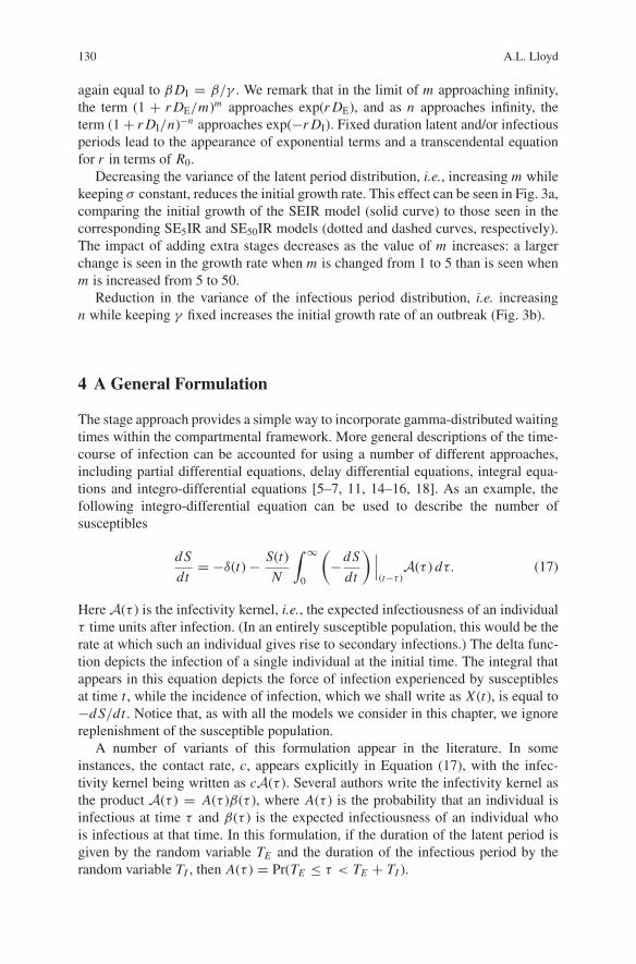
3.2 More General Compartmental Models: GammaDistributed Latent and Infectious Periods

An individual’s chance of recovery is not constant over time: typically, the recov-ery rate increases over time. In terms of a mathematical model, this leads to thecomplication that the times at which different individuals became infected must betracked. In contrast, the constant rate assumptions of the SIR and SEIR modelsare mathematically convenient as their rates of recovery and loss of latency can bewritten just in terms of the current numbers of infectives and exposeds.

A mathematical trick [1, 10, 17] allows the inclusion of non-exponential distri-butions within the compartmental framework. The infective class can be subdividedinto n stages, arranged in series. Newly infected individuals enter the first infec-tive stage, pass through each in turn, and recover upon leaving the nth stage. It isassumed that progression between stages occurs at constant per-capita rate, leadingto an exponential waiting time in each stage and allowing movement between stagesto be described by a linear system of differential equations. The stage approachallows the modeler to retain the convenience of the differential equation approach,albeit at the cost of an increased number of state variables and hence dimensionalityof the model.

In the simplest setting, the average waiting time (or equivalently the departurerate) in each stage is assumed to be equal: the overall infectious period is thendescribed by the sum of n independent exponential distributions, i.e. infectiousperiods are gamma distributed [10, 17] with shape parameter n, as illustrated inFig. 2. To allow comparison between models with different numbers of stages, theaverage duration of infectiousness is often held fixed, meaning that the departurerate is equal to nγ for each stage. In a similar way, a non-exponential latent periodcan be described by the use of m exposed stages. A general form of the SEIR model,which we dub the SEmInR model, is then given by

dS/dt = −βSI/N (9)

dE1/dt = βSI/N − mσ E1 (10)

dE2/dt = mσ E1 − mσ E2 (11)...

dEm/dt = mσ Em−1 − mσ Em (12)

dI1/dt = mσ Em − nγ I1 (13)

dI2/dt = nγ I1 − nγ I2 (14)...

dIn/dt = nγ In−1 − nγ In. (15)

Here I = I1 + I2 + · · · + In is the total number of infectives. We remark thatthe SEmInR model has just two extra parameters compared to the SEIR model, and

Sensitivity of Model-Based Epidemiological Parameter Estimation 129

0 1 2 3 4 5time, t

0

0.25

0.5

0.75

1

1.25

1.5

pdf,

f(t)

Fig. 2 Gamma distributed infectious periods. The graph illustrates the probability density function(pdf) of gamma distributions with n = 1 (dotted curve), n = 2 (dot-dashed curve), n = 5 (dashedcurve) or n = 50 (solid curve) stages. In each case, the average duration of infection DI is twodays. The variances of the gamma distributions are given by DI

2/n. As discussed in the text, forlarge n, the gamma distribution approaches a normal distribution: for comparison, the curve withcircles depicts a normal distribution with mean and variance equal to those of the n = 50 gammadistribution

that if n = m = 1, the model reduces to the standard SEIR model. If either mor n is large, then, by the Central Limit Theorem, the relevant gamma distributionbecomes approximately normal (see Fig. 2). In the limit m → ∞ or n → ∞, eitherthe exposed or infectious period distribution becomes of fixed duration.

More general distributions can be described using variations of the stage device,for instance by having unequal movement rates or more complicated arrangementsof stages, such as stages in parallel as well as in series. Furthermore, the infec-tiousness of different stages can be allowed to vary, giving a transmission term ofthe form Σiβi S Ii/N . In some instances, the stages are identified with biologically-defined different stages of an infection, as, for example, in the case of a numberof models for HIV [23]. But we emphasize that, in general, the stages are amathematical device and need not have any biological interpretation.

Linearization of the model (9)–(15) gives the growth rate (of both prevalence andincidence) as the dominant root of the equation

γ R0

{1 −(

1 + r DI

n

)−n}

= r

(1 + r DE

m

)m

. (16)

This equation is equivalent to Equation (9) of Anderson and Watson [1], butLloyd [21] employed this version in which $R 0$ appears explicitly. Here R0 is

130 A.L. Lloyd

again equal to βDI = β/γ . We remark that in the limit of m approaching infinity,the term (1 + r DE/m)m approaches exp(r DE), and as n approaches infinity, theterm (1 + r DI/n)−n approaches exp(−r DI). Fixed duration latent and/or infectiousperiods lead to the appearance of exponential terms and a transcendental equationfor r in terms of R0.

Decreasing the variance of the latent period distribution, i.e., increasing m whilekeeping σ constant, reduces the initial growth rate. This effect can be seen in Fig. 3a,comparing the initial growth of the SEIR model (solid curve) to those seen in thecorresponding SE5IR and SE50IR models (dotted and dashed curves, respectively).The impact of adding extra stages decreases as the value of m increases: a largerchange is seen in the growth rate when m is changed from 1 to 5 than is seen whenm is increased from 5 to 50.

Reduction in the variance of the infectious period distribution, i.e. increasingn while keeping γ fixed increases the initial growth rate of an outbreak (Fig. 3b).

4 A General Formulation

The stage approach provides a simple way to incorporate gamma-distributed waitingtimes within the compartmental framework. More general descriptions of the time-course of infection can be accounted for using a number of different approaches,including partial differential equations, delay differential equations, integral equa-tions and integro-differential equations [5–7, 11, 14–16, 18]. As an example, thefollowing integro-differential equation can be used to describe the number ofsusceptibles

d S

dt= −δ(t) − S(t)

N

∫ ∞

0

(−d S

dt

) ∣∣∣(t−τ )

A(τ ) dτ. (17)

Here A(τ ) is the infectivity kernel, i.e., the expected infectiousness of an individualτ time units after infection. (In an entirely susceptible population, this would be therate at which such an individual gives rise to secondary infections.) The delta func-tion depicts the infection of a single individual at the initial time. The integral thatappears in this equation depicts the force of infection experienced by susceptiblesat time t , while the incidence of infection, which we shall write as X (t), is equal to−d S/dt . Notice that, as with all the models we consider in this chapter, we ignorereplenishment of the susceptible population.

A number of variants of this formulation appear in the literature. In someinstances, the contact rate, c, appears explicitly in Equation (17), with the infec-tivity kernel being written as cA(τ ). Several authors write the infectivity kernel asthe product A(τ ) = A(τ )β(τ ), where A(τ ) is the probability that an individual isinfectious at time τ and β(τ ) is the expected infectiousness of an individual whois infectious at that time. In this formulation, if the duration of the latent period isgiven by the random variable TE and the duration of the infectious period by therandom variable TI , then A(τ ) = Pr(TE ≤ τ < TE + TI ).

Sensitivity of Model-Based Epidemiological Parameter Estimation 131

0 20 40 60 80 100time (days)

0

10

20

30

40

50

I (t

) (t

hous

ands

)

0 5 10 15 20time (days)

1

10

100

1000

I (t

)

(a)

0 10 20 30 40 50time (days)

0

20

40

60

80

I (t

) (t

hous

ands

)

0 2 4 5 7 8

time (days)

1

10

100

1000

I (t

)(b)

1 3 6

Fig. 3 Impact of distributional assumptions on epidemic behavior seen in SIR and SEIR-typemodels. Panel (a) shows the impact of the latent period distribution in SEIR-type models. In eachcase the infectious period is exponentially distributed. Solid curve: exponentially-distributed latentperiod (SEIR model). Dotted and dashed curves: gamma-distributed latent period, with m = 5 andm = 50 exposed stages (SE5IR and SE50IR models), respectively. Panel (b) depicts the effect ofvarious descriptions of the infectious period in SIR-type models (no latent period). Solid curve:exponentially distributed infectious period (SIR model). Dotted curve: gamma-distributed infec-tious period with n = 2 stages. Dot-dashed curve: gamma-distributed infectious period with n = 5stages. Dashed curve: gamma-distributed infectious period with n = 50 stages. For both panels(a) and (b), the average infectious period DI is taken to be 5 days, R0 is 5, and, where relevant, thelatent period has an average duration of DE = 2 days. At the initial time, the entire population ofN = 106 is susceptible to the infection, except for one individual who is taken to have just becomeinfectious. The insets focus on the early behavior, including the phase when the behavior can bewell approximated by a linear model

The compartmental models described in previous sections can be recast in termsof an infectivity kernel. For the SIR model, the constant level of infectivity over anexponentially distributed infectious period of average duration 1/γ gives

A(τ ) = βe−γ τ , (18)

132 A.L. Lloyd

and for the corresponding SEIR model, with average duration of latency DE equalto 1/σ , we have

A(τ ) ={

βσ

γ − σ

(e−στ − e−γ τ

)if σ �= γ

βγ τe−γ τ if σ = γ.(19)

The basic reproductive number for this model is given by

R0 =∫ ∞

0A(τ ) dτ. (20)

During the early stages of an outbreak, S(t) ≈ N , and use of the approximationS(t) = N gives the following linear integral equation for the incidence

X (t) = δ(t) +∫ ∞

0X (t − τ )A(τ ) dτ. (21)

Substitution of an exponentially growing form for the incidence, X (t) = X (0)ert ,for t ≥ 0 gives the equation

1 =∫ ∞

0e−rτA(τ ) dτ, (22)

which can be solved for the rate r at which incidence grows. This equation is thefamiliar Euler-Lotka formula from demographic theory [see, for example, 30].

The integral that appears in Equation (22) is the Laplace transform of the infec-tivity kernel. Yan [34] derived a relationship between R0 and r for a general class ofinfectivity kernels for which the random variables describing the latent and infec-tious periods, TE and TI , are independent and under the assumption that secondaryinfections arise at constant rate β over the duration of the infectious period. Assum-ing that the Laplace transforms of the distributions of both TE and TI exist, andwriting them as LE (r ) and LI (r ), Yan obtained the following general result

R0 = DI

LE (r )L∗I (r )

. (23)

Here, L∗I (r ) = (1 − LI (r ))/r .

All of the relationships between R0 and r obtained from compartmental modelsin the earlier sections of this chapter can be obtained as special cases of this result.In particular, the earlier Equation (16) can be seen as a special case of Yan’s generalresult and holds for general gamma distributed latent and infectious periods (i.e.,with any positive shape parameters—not just integers).

Sensitivity of Model-Based Epidemiological Parameter Estimation 133

5 Comparing R0 Estimates Obtained Using Different Models

The relationships between R0 and r described in previous sections, obtained froma number of SIR and SEIR-type models, are collected together in Table 1. It isimmediately clear that use of the SIR-based formula provides a lower estimate ofR0 than would be obtained using the SEIR-based formula [21, 25, 33]. Ignoring aninfection’s latent period leads to underestimates of R0, with the underestimate beingmore serious for faster growth rates or longer durations of latency (e.g., compareTables 2, 3 and 4).

The origin of the underestimate is clear from the analysis and simulations pre-sented earlier: given the same values for the transmission parameter and the average

Table 1 Relationships between the initial growth rate r and the basic reproductive number R0

obtained from various models

Model Formula

SIR R0 = 1 + r DI

SInR R0 = r DI1 − (1 + r DI/n)−n

SI∞R R0 = r DI

1 − e−r DI

SEIR R0 = (1 + r DI) (1 + r DE)

SEI∞R R0 = r DI(1 + r DE)1 − e−r DI

SEm IR R0 = (1 + r DI) (1 + r DE/m)m

SEm InR R0 = r DI (1 + r DE/m)m

1 − (1 + r DI/n)−n

SE∞IR R0 = (1 + r DI) er DE

SE∞I∞R R0 = r DIer DE

1 − e−r DI

Table 2 R0 and pc estimates obtained using various models when r = 0.04 day−1, DE = 3 daysand DI = 8 days. These parameters were chosen to be similar to those employed in [8] to describeSARS

Model R0 estimate Control fraction pc

SIR 1.32 0.242SI5R 1.20 0.167SI∞R 1.17 0.144SEIR 1.48 0.324SEI∞R 1.31 0.236SE5IR 1.49 0.327SE5I5R 1.35 0.260SE∞IR 1.49 0.328SE∞I∞R 1.32 0.241

134 A.L. Lloyd

Table 3 Impact of faster growth rate on R0 estimates. Here, r = 0.12 day−1, while DE = 3 daysand DI = 8 days take the same values as in the previous table

Model R0 estimate Control fraction pc

SIR 1.96 0.490SI5R 1.64 0.391SI∞R 1.56 0.357SEIR 2.67 0.625SEI∞R 2.12 0.527SE5IR 2.77 0.640SE5I5R 2.33 0.570SE∞IR 2.81 0.644SE∞I∞R 2.23 0.552

duration of infectiousness, the SEIR model would predict a lower growth rate thanthe corresponding SIR model. Consequently, in order to achieve the same growthrate in this forward problem setting, a higher transmission parameter, and hence R0,must be used in the SEIR model than in the corresponding SIR model.

Larger estimates of the basic reproductive number are obtained when non-exponential descriptions of the latent period distribution are used. Because thefunction (1 + a/x)x is monotonic increasing for a > 0, increasing the number oflatent stages m (i.e., reducing the variance of the latent period distribution) increasesthe estimate [21, 27, 33, 34], with the estimate that employs a fixed duration oflatency (i.e., m → ∞) providing an upper bound. On the other hand, lower estimatesof the basic reproductive number are obtained when the number of infectious stagesn is increased [21, 27, 33, 34], with the estimate obtained using a fixed duration ofinfectiousness (i.e., n → ∞) being a lower bound.

Because estimates of R0 are often used to determine the severity of measuresneeded to bring an outbreak under control, assumptions made about the timecourseof infection can have important public health consequences [21, 33]. If the aim ofcontrol is to bring the basic reproductive number below one, the transmissibilityof the infection must be reduced by a factor of pc = 1 − 1/R0. Here, we call pc

the control fraction. (In the context of mass vaccination, pc is called the critical

Table 4 Impact of longer average duration of latency on R0 estimates. Here, DE = 5 days, whiler = 0.12 day−1 and DI = 8 days, as in the previous table

Model R0 estimate Control fraction pc

SIR 1.96 0.490SInR 1.64 0.391SI∞R 1.56 0.357SEIR 3.14 0.681SEI∞R 2.49 0.598SEm IR 3.45 0.710SEm InR 2.89 0.655SE∞IR 3.57 0.720SE∞I∞R 2.83 0.647

Sensitivity of Model-Based Epidemiological Parameter Estimation 135

vaccination fraction.) As we have seen, use of SIR models underestimates the basicreproductive number and hence leads to lower estimates of pc compared to thoseobtained using SEIR models. This could be a serious problem as it leads to anoverly optimistic prediction of the strength of control needed to curtail an outbreak:a control measure that, on the basis of the incorrect model, is predicted to succeedcould, instead, be doomed to failure [21].

We first illustrate these results by providing a few examples using a growth rateand durations of latency and infectiousness based roughly on a SARS modelingstudy of Chowell et al. [8]. (The study of Chowell et al. accounted for treatmentand isolation, using a more complex model than those employed here, so directcomparisons cannot be made.) Table 2 shows estimates obtained for an observedgrowth rate of 0.04 per day, assuming a three day average duration of latency and aneight day average duration of infectiousness. We imagine that details of how latentand infectious periods are distributed about their means are unknown, and so presentestimates based on a number of models. This provides an indication of the degreeof uncertainty that arises from incomplete knowledge of these distributions. (Herewe ignore the additional complication that the estimate of r would also have someuncertainty.) For this example, comparing the SIR and SEIR-based estimates, wesee that ignoring the latent period leads to R0 being underestimated by about 10%.This translates into a 25% underestimate of the control fraction.

Interestingly, for this set of parameters, the distribution of the latent period (pro-vided that one is used in the first place) has little impact on the estimates, whilethe infectious period distribution has a more noticeable effect. In this case the lattereffect is sufficiently large to offset the differences introduced by ignoring a latentperiod: the estimates obtained using the SIR and the SE∞I∞R models are almostidentical.

For a more rapidly growing outbreak, in which r = 0.12 day−1 is three timeslarger than its previous value, the SIR model underestimates R0 by a larger amount,roughly 25%, compared to the SEIR estimate (Table 3). This corresponds to a 22%underestimate of the control fraction. We remark that while this underestimate isslightly smaller in percentage terms than that seen under the previous set of param-eters, it is larger in absolute terms. Also, given that the required level of control ishigher, the increase in effectiveness needed to go from the SIR-based estimate of pc

to the SEIR-based estimate may be much more difficult to achieve. For this set ofparameters, the form of the latent period distribution has a more noticeable impact.

If the infection is both more rapidly growing and has a longer duration of latencythe underestimate of R0 is more severe. In the example of Table 4, in which theaverage duration of latency has been raised from 3 to 5 days, use of the SIR modelunderestimates R0 by roughly 38% of the SEIR-based estimate. The two estimatesof the control fraction are 0.490 (SIR) and 0.681 (SEIR).

Figure 4 shows how estimates of R0 obtained using the SEmInR model dependin turn on each of the quantities DE, DI, m, n and r for a situation corresponding toTable 4. We take DE = 5 days, DI = 8 days, r = 0.12 day −1, m = 5 and n = 5as a baseline, and vary just one of these at a time. As discussed above, the estimateof R0 increases with m, DE, DI and r , but decreases with n. We also see that the

136 A.L. Lloyd

1 5 10 15m or n

2.5

3

3.5

R0

0 2 4 6 8 10DE or DI

1

2

3

4

5R

0

0 0.05 0.1 0.15 0.2 0.25r

2

4

6

8

R0

(a)

(c)

(b)

Fig. 4 Sensitivity of the R0 estimate to variations in single parameter values or the initial growthrate. One of five quantities is varied in turn: Panel (a) DE (solid curve) or DI (dashed curve); Panel(b) m (solid curve) or n (dashed curve); Panel (c) r . The four other values are taken from thebaseline set of DE = 5 days, DI = 8 days, m = 5, n = 5, and r = 0.12 day −1

sensitivity of the estimate varies with these parameters, for instance, the R0 estimateis less sensitive to m for larger values of m.

A dramatic example of the potential for the underestimation of R0 was providedby Nowak et al. [25] in a within-host setting that can be modeled using virus dynam-ics models that are directly analogous to the epidemiological models consideredhere. The initial growth rate of simian immunodeficiency virus (SIV) in one par-ticular animal in an experimental infection study was found to be 2.2 day−1 andthe average duration of infectiousness (of SIV infected cells) was 1.35 days. Useof the SIR model gave an estimate of R0 = 4.0, the SEIR model, assuming a oneday latent period (i.e., the delay between a cell becoming infected and becominginfectious), gave R0 = 13, while the SE∞IR model gave R0 = 36. We remark on thelarge impact of the distribution of the latent period in this instance. In terms of con-trol fractions, the three models predict values of 0.75 (SIR), 0.92 (SEIR) and 0.97(SE∞IR). While there may be hope in achieving a 75% reduction in transmissibility,a 92 or 97% reduction would be much harder to achieve. In this case, use of the SIRmodel gives a wildly optimistic picture of the effectiveness required of a controlmeasure.

Sensitivity of Model-Based Epidemiological Parameter Estimation 137

If the latent period in this within-host example was instead assumed to be 0.5days, the effect would be reduced, with the SEIR and SE∞IR-based estimates ofR0 falling to 8.3 and 12, respectively. These values are still considerably larger thanthe SIR-based estimate of 4.0, and the estimate is still highly sensitive to the distri-bution of the latent period. The corresponding control fractions are 0.88 and 0.92,respectively.

6 Sensitivity Analysis

The numerical examples presented above give an idea of the dependency of R0

estimates on parameter values in particular settings, but a more systematic explo-ration can be achieved using sensitivity analysis. It is straightforward to calculatethe partial derivatives of the estimated value of R0 as provided by the SEmInR model(i.e., using Equation 16) with respect to the parameters DE, DI, m, n, and the initialgrowth rate r . The elasticity Ex , which approximates the fractional change in the R0

estimate that results from a unit fractional change in parameter x (while keeping allother parameters constant), is given by Ex = (x/R0) · ∂ R0/∂x . The elasticities forthe quantities of interest are

EDE = r DE

1 + r DE/m(24)

EDI = 1 − r DI

(1 + r DI/n)((1 + r DI/n)n − 1

) (25)

Em = m ln

(1 + r DE

m

)− r DE

1 + r DE/m(26)

En = 1

(1 + r DI/n)n − 1

(−n ln (1 + r DI/n) + r DI

1 + r DI/n

)(27)

Er = 1 + r DE

1 + r DE/m− r DI

(1 + r DI/n)((1 + r DI/n)n − 1

) . (28)

We remark that if the curves that appear in Fig. 4 were replotted on log-log axes,these elasticities would describe the slopes of these new graphs.

The signs of the elasticities confirm the earlier discussion of how the estimateof R0 varies as parameter values are changed. Clearly EDE is positive, meaningthat increases in DE lead to larger estimates of R0. EDI is also seen to be positive,since the second term in Equation (25) is smaller than one for positive values ofthe parameters r , DI and n: increases in DI again lead to larger estimates of R0.Em is seen to be positive when m, r and DE are positive because the functionm ln(1 + x/m) − x/(1 + x/m) is monotonic increasing in x and takes the value 0when x equals zero. A similar argument shows that En is negative. Finally, Er equalsthe sum of EDE and EDI and so is positive, and is greater than either EDE or EDI .

138 A.L. Lloyd

A little algebra shows that EDE is an increasing function of r , DE or m, i.e., theelasticity of the R0 estimate with respect to DE increases with these parameters. EDI

is an increasing function of r or DI, but parameter sets can be found for which it isnon-monotonic as n changes. Em increases with r or DE, but can be non-monotonicas m changes. En can be non-monotonic as r or DI changes. As before, Er inheritsthe properties of EDE and EDI , and so increases with DE, DI, m or r , but need notbe a monotonic function of n.

For the parameters of Table 2 and when m = n = 1 we find that the elasticitiesare given by EDE = 0.107, EDI = 0.242, Em = 0.006, En = −0.110, and Er =0.350. If, instead, we take m = n = 5 the elasticities are EDE = 0.117, EDI =0.173, Em = 0.001, En = −0.026, and Er = 0.290. In both cases, the R0 estimateis more sensitive to changes in DI than to changes in DE, and here we see thatsensitivities to m and n are of smaller magnitude for larger values of m and n, whilethe sensitivity to DE increases with increasing m and the sensitivity to DI decreaseswith increasing n.

Whether the estimate is more sensitive to changes in DE or DI (or to m or n)depends on the values of the parameters. For example, if the parameters of Table4 are taken, and m = n = 1 is assumed, the elasticities are EDE = 0.375, EDI =0.490, Em = 0.095, En = −0.191, and Er = 0.865. If, instead, we assumed m =n = 5, the estimate of R0 would be more sensitive to DE than to DI (EDE = 0.536and EDI = 0.427), and if we took m = 1 and n = 5, the estimate would be moresensitive to m than to n (Em = 0.095 and En = −0.052).

One important question that the elasticities discussed in this section do notaddress is the impact of neglecting the latent period entirely. Having said this, theyare useful in understanding how uncertainties in the average duration of the latent orinfectious period, the dispersions of these distributions, as described by m or n, orthe initial growth rate impact the estimation of R0 in the SEmInR model framework.

7 Discussion

The importance of non-exponential infectious periods and time-varying infectious-ness has long been appreciated for chronic infections, such as HIV, for which aconstant recovery rate assumption is clearly untenable [5–7, 16, 23, 24]. Even inthe setting of models of acute infections, there is a surprisingly long history of theuse of more complex models: Kermack and McKendrick’s groundbreaking paperof 1927 [18] contains an integral equation formulation along the lines of Equation(17), and Bailey [3] used the stage approach and the resulting SEmInR model. Theimportance of distributional assumptions has typically been viewed in terms of theirimpact on the behavior of a model for a given set of parameters (i.e., the forwardproblem): effects such as the slower growth of epidemics for infections with latencyhave long been appreciated.

The impact of distributional assumptions on the inverse problem, (i.e., the esti-mation of parameters given the observed behavior), however, appears to have onlyrecently become fully appreciated. Nowak et al. [25] showed that the SIR-based

Sensitivity of Model-Based Epidemiological Parameter Estimation 139

estimates of the within-host basic reproductive number of SIV (simian immunod-eficiency virus) severely underestimated R0 when compared to estimates obtainedusing more realistic SEIR models. Little et al. [20] carried out a similar analysis inthe setting of HIV infection. Much of the theory and results discussed in this chap-ter were laid out by Lloyd [21], in the setting of within-host infections, although,because of the obvious correspondence between within-host and between-host mod-els, the application to estimation in the epidemiological setting was highlighted [seealso the discussion of 22]. Wearing et al. [33] further illustrated these results inan epidemiological setting, and broadened consideration to include estimation ofR0 based on data from the entire outbreak, as discussed below. A complementaryapproach was taken by Wallinga and Lipsitch [31] and Roberts and Heesterbeek[27], who examined the relationship between R0 and r in terms of the generationinterval of the infection (i.e., the time between an individual becoming infected andthe secondary infections that they cause). Both of these studies considered gammadistributed latent and infectious periods, including the exponential and fixed dura-tion cases, giving equivalent results to those discussed here. Additional familiesof distributions were also considered, including trapezoidal infectivity kernels [27]and normally distributed generation intervals [31]. Yan [34] provided a comprehen-sive analysis that encompassed and unified most of these earlier studies, derivinggeneral results in terms of Laplace transforms of the latent and infectious perioddistributions.

The results presented here demonstrate that estimates of the basic reproductivenumber obtained from the initial growth rate of a disease outbreak can be sensitiveto the details of the timing of secondary infection events (i.e., to the distributionof infectious and latent periods). Such details, while clearly important, are oftendifficult to obtain. Data that identifies when an individual was exposed to infectionand when their secondary transmissions occurred, such as family-based transmis-sion studies or contact tracing data—even if incomplete—can be highly informativein this regard [2, 4, 12, 13]. It is important to realize that models are often framed interms of transmission status, e.g. whether an individual is infectious, while data mayreflect disease status, e.g. whether an individual is symptomatic or not. This distinc-tion is important in the interpretation of the most commonly available distributionaldata, namely the incubation period distribution [28], because the incubation periodof an infection may not, and often does not, correspond to its latent period [see, forexample, 29].

In this chapter we only considered the estimation of R0 from initial growth data,but similar results are obtained if models are instead fitted to data obtained over theentirety of an outbreak [33]. This makes sense given the observation that distribu-tional assumptions affect not only the initial growth rate but the whole time courseof an outbreak in the forward problem (see Figs. 1 and 3). Whole-outbreak data isconsiderably more informative than initial growth data, for instance Wearing et al.[33] used a least-squares approach to estimate β, DE and DI as well as the shapeparameters m and n of the gamma distributions describing latency and infectious-ness. Initial growth rate data, on the other hand, does not even allow β and γ tobe independently estimated. Capaldi et al. (manuscript in preparation) examine thetypes of data that allow for the estimation of different parameters in more detail.

140 A.L. Lloyd

Wearing et al. [33] also make the important observation that different estimates ofR0 can, in some instances, be obtained if initial data is used rather than data from anentire outbreak [see also 9].

If detailed information on the distribution of latent and infectious periods isabsent, caution should be taken in basing an estimate of R0 by fitting a singlemodel. The use of a number of models can provide bounds on the estimate, givingan indication of the uncertainty arising from our incomplete knowledge of the trans-mission process. Any model-based uncertainty is in addition to that which arisesfrom noise in the data—an issue that we have not discussed in this chapter—andso the most informative uncertainty estimate would account for both sources oferror. (Sensitivity calculations, such as those discussed above, can be informativein this regard.) In some instances, however, model-based uncertainty may placea much greater limit on our ability to estimate parameters. As in the within-hostexample of Nowak et al. [25], this uncertainty can be so large as to render the esti-mates almost uninformative—but at least the deficiency is exposed by the approachadvocated here.

References

1. Anderson DA, Watson RK (1980) On the spread of disease with gamma distributed latent andinfectious periods. Biometrika 67:191–198.

2. Bailey NTJ (1954) A statistical method for estimating the periods of incubation and infectionof an infectious disease. Nature 174:139–140.

3. Bailey NTJ (1964) Some stochastic models for small epidemics in large populations. Appl.Stat. 13:9–19.

4. Bailey NTJ (1975) The Mathematical Theory of Infectious Diseases. Griffin, London.5. Blythe SP, Anderson RM (1988) Variable infectiousness in HIV transmission models. IMA J.

Math. Appl. Med. Biol. 5:181–200.6. Blythe SP, Anderson RM (1988) Distributed incubation and infectious periods in models of

the transmission dynamics of the human immunodeficiency virus (HIV). IMA J. Math. Appl.Med. Biol. 5:1–19.

7. Castillo-Chavez C, Cooke K, Huang W, Levin SA (1989) On the role of long incubationperiods in the dynamics of HIV/AIDS, Part 1: Single population models. J. Math. Biol. 27:373–398.

8. Chowell G, Fenimore PW, Castillo-Garsow MA, Castillo-Chavez C (2003) SARS outbreaks inOntario, Hong Kong and Singapore: the role of diagnosis and isolation as a control mechanism.J. Theor. Biol. 224:1–8.

9. Chowell G, Nishiura H, Bettencourt LMA (2007) Comparative estimation of the reproduc-tion number for pandemic influenza from daily case notification data. J. R. Soc. Interface 4:155–166.

10. Cox DR, Miller HD (1965) The Theory of Stochastic Processes. Methuen, London.11. Diekmann O, Heesterbeek JAP (2000) Mathematical Epidemiology of Infectious Diseases.

John Wiley & Son, Chichester.12. Donnelly CA, Ghani AC, Leung GM, Hedley AJ, Fraser C, Riley S, Abu-Raddad LJ, Ho L-M,

Thach T-Q, Chau P, Chan K-P, Lam T-H, Tse L-Y, Tsang T, Liu S-H, Kong JHB, Lau EMC,Ferguson NM, Anderson RM (2003) Epidemiological determinants of spread of causal agentof severe acute respiratory syndrome in Hong Kong. Lancet 361:1761–1766.

Sensitivity of Model-Based Epidemiological Parameter Estimation 141

13. Haydon DT, Chase-Topping M, Shaw DJ, Matthews L, Friar JK, Wilesmith J, WoolhouseMEJ (2003) The construction and analysis of epidemic trees with reference to the 2001 UKfoot-and-mouth outbreak. Proc. R. Soc. Lond. B 269:121–127.

14. Hethcote HW, Tudor DW (1980) Integral equation models for endemic infectious diseases. J.Math. Biol. 9:37–47.

15. Hoppensteadt F (1974) An age dependent epidemic model. J. Franklin Inst. 297:325–333.16. Hyman JM, Stanley EA (1988) Using mathematical models to understand the AIDS epidemic.

Math. Biosci. 90:415–473.17. Jensen A (1948) An elucidation of Erlang’s statistical works through the theory of stochastic

processes. In E. Brockmeyer, H. L. Halstrøm, and A. Jensen, editors, The Life and Works ofA. K. Erlang, pages 23–100. The Copenhagen Telephone Company, Copenhagen.

18. Kermack WO, McKendrick AG (1927) A contribution to the mathematical theory ofepidemics. Proc. R. Soc. Lond. A 115:700–721.

19. Lipsitch M, Cohen T, Cooper B, Robins JM, Ma S, James L, Gopalakrishna G, Chew SK, TanCC, Samore MH, Fisman D, Murray M (2003) Transmission dynamics and control of severeacute respiratory syndrome. Science 300:1966–1970.

20. Little SJ, McLean AR, Spina CA, Richman DD, Havlir DV (1999) Viral dynamics of acuteHIV-1 infection. J. Exp. Med. 190:841–850.

21. Lloyd AL (2001) The dependence of viral parameter estimates on the assumed viral life cycle:Limitations of studies of viral load data. Proc. R. Soc. Lond. B 268:847–854.

22. Lloyd AL (2001) Destabilization of epidemic models with the inclusion of realisticdistributions of infections periods. Proc. R. Soc. Lond. B 268:985–993.

23. Longini IM, Clark WS, Byers RH, Ward JW, Darrow WW, Lemp GF, Hethcote HW (1989)Statistical analysis of the stages of HIV infection using a Markov model. Stat. Med. 8:831–843.

24. Malice M-P, Kryscio RJ (1989) On the role of variable incubation periods in simple epidemicmodels. IMA J. Math. Appl. Med. Biol. 6:233–242.

25. Nowak MA, Lloyd AL, Vasquez GM, Wiltrout TA, Wahl LM, Bischofberger N, Williams J,Kinter A, Fauci AS, Hirsch VM, Lifson JD (1997) Viral dynamics of primary viremia andantiretroviral therapy in simian immunodeficiency virus infection. J. Virol. 71:7518–25.

26. Riley S, Fraser C, Donnelly CA, Ghani AC, Abu-Raddad LJ, Hedley AJ, Leung GM, Ho L-M,Lam T-H, Thach T-Q, Chau P, Chan K-P, Lo S-V, Leung P-Y,Tsang T, Ho W, Lee K-H, LauEMC, Ferguson NM, Anderson RM (2003) Transmission dynamics of the etiological agent ofSARS in Hong Kong: Impact of public health interventions. Science 300:1961–1966.

27. Roberts MG, Heesterbeek JAP (2007) Model-consistent estimation of the basic reproductionnumber from the incidence of an emerging infection. J. Math. Biol. 55:803–816.

28. Sartwell PE (1950) The distribution of incubation periods of infectious disease. Am. J. Hygiene51:310–318.

29. Sartwell PE (1966) The incubation period and the dynamics of infectious disease. Am. J.Epidemiol. 83:204–216.

30. Smith D, Keyfitz N (1977) Mathematical Demography. Selected Papers. Biomathematics,Volume 6. Springer-Verlag, Berlin.

31. Wallinga J, Lipsitch M (2007) How generation intervals shape the relationship between growthrates and reproductive numbers. Proc. R. Soc. Lond. B 274:599–604.

32. Wallinga J, Teunis P (2004) Different epidemic curves for severe acute respiratory syndromereveal similar impacts of control measures. Am. J. Epidemiol. 160:509–516.

33. Wearing HJ, Rohani P, Keeling M (2005) Appropriate models for the management ofinfectious diseases. PLoS Medicine 2(7):e174.

34. Yan P (2008) Separate roles of the latent and infectious periods in shaping the relation betweenthe basic reproduction number and the intrinsic growth rate of infectious disease outbreaks. J.Theor. Biol. 251:238–252.