Sequencing and scheduling in the sheet metal shopcdn.intechweb.org/pdfs/629.pdf · Sequencing and scheduling in the sheet metal shop ... a punch press or cut with a laser machine

20

Sequencing and scheduling in the sheet metal shop

B. Verlinden1, D. Cattrysse1, H. Crauwels2, J. Duflou1 and D. Van Oudheusden1

1K.U.Leuven, Centre for Industrial Management 2Hogeschool voor Wetenschap en Kunst, De Nayer Instituut

Belgium

1. Introduction

1.1 History

Sheet metal operations have been in existence since 8000 B.C. (Fries-Knoblach, 1999). Due to its long history, sheet metalworking is, unfortunately, often seen as archaic and uninteresting. That metal sheets can be transformed with the aid of robust machines into fancy consumer products with tight tolerances is inconceivable to many. Yet, sheet metal operations are used for producing both structural components and durable consumer goods. Nowadays, sheet metal parts are widely present in different daily life products. During the past decades, scientific research in the field of sheet metal operations has been booming and international conferences on different sheet metal topics attract numerous attendants. Both industry and the academic community recognize the importance of continuing improvement in sheet metal operations. Thirty years ago, the rapid advance of computer systems triggered the introduction of automation in manufacturing environments. Also for sheet metal operations the use of computer systems has become indispensable to survive. Computer aided design (CAD) and computer aided manufacturing (CAM) systems are widely present in sheet metal production environments. At the earliest design stage, CAD systems are used to computerize the whole process of drawing and redrawing the desired part. Most modern CAD systems allow to build up a part from several re-usable 3D components, thus automating to a large extent the time consuming design process. The use of computers has also entered the manufacturing stage through computer aided manufacturing. The CAD file is converted into a sequence of processes for manufacture on a numerically controlled (NC) machine. The use of computers helps operators in automating different steps of the production process. As far as planning is concerned, most attention is focused on the computerization of sheet metal process planning. Production planning proper received much less attention due to a long tradition of experience-based production planning.

1.2 Scope of the research

If one queries the internet for sheet metal operations, numerous entries on processes are found, for instance on laser cutting, punching, deep drawing, bending, incremental forming,

Source: Multiprocessor Scheduling: Theory and Applications, Book edited by Eugene Levner,ISBN 978-3-902613-02-8, pp.436, December 2007, Itech Education and Publishing, Vienna, Austria

Ope

nA

cces

sD

atab

ase

ww

w.i-

tech

onlin

e.co

m

Multiprocessor Scheduling: Theory and Applications 346

etc. Since many different sheet metal production processes and production environments can be identified, it is important to clearly delineate the scope of the research. The research as described in this chapter focuses on sheet metal operations in a flow shop environment (Figure 1). As far as the production processes are concerned, only laser cutting and air bending are considered.

Figure 1. Sheet metal operations

Figure 2. Typical sheet metal parts (a) complex part; (b) standard profile

Figure 3. The air bending principle

All parts follow a unidirectional flow in the sheet metal shop. In a preliminary stage, a large standard metal sheet or coil is cut to the right dimensions by using a pair of automated scissors (the shearing operation). Next, in the cutting stage, the unfolded blank of a part is punched with a punch press or cut with a laser machine. After cutting, the parts are bent

Sequencing and scheduling in the sheet metal shop 347

and transformed into 3D products. Air bending is used for this purpose. The air bending machine or press brake consists of a fixed bed on which the dies are fastened and a vertically movable ram (driven by hydraulic cylinders) on which the punches are mounted. A vertical force causes the ram to move down, forcing the sheet into the die, creating the bend line. The larger the vertical force, the smaller the bend angle (Figure 3). To produce a bend line of a part, a punch and die are required (called a tool set). The geometrical properties of the bend line (i.e. internal radius, bend allowance, type of profile, etc.) determine the characteristics of the required tool set. Punches and dies are supplied in sections (segments) for easy handling and quick set-up. If a long tool is needed, different segments are required. A combination of different segments to produce a single bend line is called a station. If a part consists of multiple bend lines, multiple stations are usually required (e.g. one station per bend line). Some stations may be used to produce several bend lines, while other stations can only be used for very specific lines. If a part requires different stations, all stations are positioned on the press brake with the required space between them, resulting in a production layout (Figure 4). A production layout can be used for bending several parts (depending on the geometrical properties of the part). This chapter mainly focuses on combinatorial optimization models and algorithms of use to production planning in Belgian small to medium-sized enterprises. Typically, in a Belgian SME, a single laser machine and press brake are available for production. Batch sizes range from a single workpiece to larger series (200 parts).

Figure 4. Press brake with a production layout consisting of three stations (every station is built up with different segments)

1.3 Outline

The research as described in this chapter evolved from a project in cooperation with a large sheet metal machine constructor and has been carried out by members of the Centre for Industrial Management, K.U.Leuven. The main goal of the project was to tackle a series of practical problems in a typical sheet metal shop. The chapter has six sections. Section 2 discusses some process planning issues for sheet metal laser cutting and air bending. An overview is given and relevant literature is mentioned. Section 3 elaborates on the tooling layout problem for air bending. The problem


is analyzed and several solution procedures are proposed. Section 4 analyzes the production planning problem for air bending. A traveling purchaser problem approach (TPP) and a generalized traveling salesperson problem approach (GTSP) are proposed to reformulate the air bending production planning problem. Section 5 discusses production planning integration of laser cutting with air bending. The problems are highlighted and mathematical models are proposed. Computational results are discussed for a number of test cases. Section 6 concludes the chapter and formulates future research topics. In the chapter, mathematical models are formulated for the different planning issues, taking into account numerous problem-specific constraints. Typically, in a first stage, optimization procedures are used to obtain overall optimal solutions, but the computational effort required to solve combinatorial problems to optimality appears to grow very fast with the size of the problem. Local search, a class of heuristic methods, is applied at that point. It allows in a straightforward way to determine good, but not necessarily optimal solutions after a limited computational effort. In the problems discussed in this chapter two classes of local search techniques are implemented: simple neighborhood search and guided local search. Neighborhood search starts with a known feasible solution and tries to improve this solution by making well-defined moves in the solution space, shifting from one neighbor to another. A move is evaluated by comparing the objective function value of the current solution to that of its neighbor. In a pure descent method, only improving moves are allowed. When no further improvement can be found, the procedure ends. All feasible moves need to be defined and the search has to be initialized with a first solution. Although good choices for the different implementation issues can improve the performance of a descent algorithm, the resulting solution is, most likely, a local optimum, not a global optimum. A classical remedy for this drawback is to perform multiple runs of the procedure starting from different initial solutions and to take the best result as final solution (multi-start descent). Another possibility is to use a combination of different neighborhood structures (variable neighborhood search), as introduced by Mladenovi & Hansen (1997). In this way, a local optimum relative to a number of neighborhoods is determined. A more specialized type of local search is guided local search (GLS). The main feature of this approach is the iterative use of local search sequences. GLS penalizes, based on a utility function, unwanted solution features at the end of a local search sequence. In this way the solution procedure may escape from a local optimum and continue the search. The interested reader is referred to Voudouris & Tsang (1999).

2. Process planning issues

Besides production planning, the authors have used combinatorial optimization techniques also for a number of sheet metal process planning aspects. Next section discusses the state of the art regarding process planning issues and summarizes some of the process planning research conducted by the authors.

2.1 Process planning for laser cutting

Past decades steel prices have been increasing, resulting in a higher material cost for sheet metal parts. Hence, the amount of waste material needs to be minimized. In order to reduce the waste material, sheet metal parts with identical characteristics (material and thickness) are, if possible, combined on a large standard sheet to obtain high sheet utilization ratios.


The problem of combining different patterns on a flat blank or coil (apart from metal, the material can be paper, cardboard, leather, wood, plastic, textile, etc.) is known as the cutting stock problem and has received much attention. Alternatively, the name nesting is used. Numerous publications and applications can be found on this topic and a wide variety of solution techniques is proposed. Research on the cutting stock problem started with Eisemann (1957) discussing the problem of minimizing losses when cutting rolls of paper, textile, metal and other materials. This trim problem aims at allocating raws to machines and setting up the different cuts in such a way that the demanded rolls are cut to the right width, minimizing the overall trimming loss. Small problems are solved by enumerating the different possibilities. Most cutting stock problems were at that time formulated as integer programming problems to be solved with standard solution procedures. An overview is given by Haessler & Sweeney (1991). Research also focused on the determination of optimal sheet layouts. For such problems one has a number of rectangular sheets that need to be filled with two-dimensional regular and irregular shapes, minimizing the waste material. In the earliest days, researchers proposed to work with encaging rectangles. Adamowicz and Albano (1976) propose a two-stage approach. In a first stage, optimal rectangular modules are produced encaging one or more parts. In the second stage those modules are positioned on a sheet, minimizing the waste material. Working with encaging rectangles can only produce a rough plan since the exact shape of the parts is not considered. When personal computers with larger computational power became available, research shifted towards the nesting of the complex parts themselves instead of encaging rectangles. Lee & Woo (1988) developed a method to seek the minimal area convex hull of two convex polygons P and Q with Q being allowed to be translated along the boundary of P. If both translation and rotation operations are allowed, the problem of finding the minimal area convex hull becomes more difficult. The interested reader is referred to Nye (2001). Nesting remains an important issue in sheet metal cutting. Different peculiarities inherent to sheet metal production have to be taken into account when nesting different unfolded blanks on a large standard sheet. Prasad (1994) proposes some heuristic algorithms for nesting irregular sheet metal parts, taking into account grain orientation, minimum bridge width (i.e. the distance between two parts should be strong enough to withhold the bending force) and maximal material utilization. Tang and Rajesham (1994) propose an algorithm taking into account the rolling direction of the part. The rolling direction influences the brittleness of the part in both traverse and rolling direction. When bending the part this can cause the bend to crack at the bending edge. Generally it is assumed that a bend made at 30° to the grain flow is enough to avoid breakage. To overcome this problem, rolling direction information is taken into account at the nesting procedure. The method proposed approximates the part by a polygon with a sufficient number of sides to represent closely the original geometric shape. A more recent overview of sheet metal nesting is given by Valvo and Licari (2007). Besides the nesting proper, other related process planning issues received attention as well. After optimal nestings are generated, the cutting technology (laser power, cutting speed, position of the focal point, cutting gas pressure, stand-off distance between nozzle and material, lead-in, piercing method, etc.) and the cutting path need to be determined (taking into account common cuts, cutting distance minimization, heat build up in the material when cutting, etc.). Fortunately for the end-user, those different issues have been


satisfactorily studied and are implemented in commercial nesting software. Such dedicated software tools allow the user to generate good nestings and to determine the cutting technology automatically.

2.2 Process planning for air bending

As for the laser cutting process, research on the bending process focuses on process planning. When a (3D) sheet metal part is produced with air bending, one starts from the unfolded blank of the required part (Figure 5). Gradually, this 2D flat blank is transformed into a 3D final workpiece by producing the different required bend lines. Different sequences are possible for producing the bend lines. Some bend sequences will cause collisions between the part, the machine and the tools while other sequences create no problems. The main goal of process planning is to determine an executable bend sequence and to select the different tools to use for each bend line, the gauging positions and the punch displacements.

Figure 5. Different unfoldings of a part

In order to determine the bend sequence, the different interactions between the part, the machine and the operator need to be investigated. For this purpose, a model is required representing the part during each of the consecutive process steps. If all geometric specifications, topological information, material characteristics and process related information would be included in such a representation model, the memory requirements could become very large. Some information, however, is redundant and only key information needs to be included. Duflou (1999) proposes a reduced foil model that contains only specific geometric information. This model also contains information regarding the topological relationships between the flange and the bend features of a part. For this purpose the part is represented by a graph with n nodes. The nodes represent the flanges, while the arcs represent the connecting features. The part can then be represented by a binary matrix, indicating whether two flanges are connected or not (Figure 6). For most parts the graph representation has to correspond with a spanning tree in the complete nxn graph. If loops are present in the graph representation scheme, a number of possibilities occur:

• the part can still be produced with air bending, but dedicated tooling will be required;


• the part can still be produced if a set of bends is simultaneously executed (so-called compulsory combined bends);

• no producible part’s unfolding can be determined: one or more bend connections need to be converted in weld connections or open seams.

The interested reader is referred to Duflou (1999). Additionally to the geometric and topological constraints, also technological constraints are enforced on the part. Non-compliance with those constraints causes the part to be infeasible to manufacture.

Figure 6. Part representation schemes (Duflou, 1999): (a) the 3D sheet metal part; (b) the unfolded blank of the part and the spanning tree; (c) the incidence matrix

Figure 7. Possible collision with (a) the punch and (b) the ram, when the bend sequence is not optimal

Thus the part representation scheme is used to determine the bend sequence and the gauging positions. The number of bend lines of the part, the number of gauging positions of the press


brake and the different possible tools to produce the part tremendously increase the number of possible bend sequences. Duflou (1999) proposes a traveling salesperson problem based method to identify feasible (near-optimal) bend sequences. To limit in this TSP approach the number of possible candidate solutions, a number of criteria is used. Amongst others, ergonomic factors and productivity criteria are taken into account when verifying the feasibility of the different bend sequences. Also hard reject criteria (unavailability of proper gauging edges, collisions, non-compliance of the part dimensions with the specified tolerances, etc.) and soft criteria (e.g. looking at the ease of workpiece handling and total resource utilization) are used to reduce the number of candidate solutions. Each criterion is assigned a weight to be included in the TSP objective function. As such, a feasible (near optimal) bend sequence is determined from the remaining candidates. Bend sequencing is often integrated with tool selection (Nguyen, 2005). For each bend line a short list of possible tools is made based on technological and geometrical constraints. The technological constraints verify if the part can technically be made with the specific tool. Geometrical constraints check if there are any foreseeable collisions (Figure 7). In general a two-phase approach is followed. In the first phase (preselection phase) all nonconforming toolsets are eliminated for each bend line, based on the technological and geometric constraints. In the second phase (refined selection phase) the preselected tools are adjusted whenever a collision occurs to suit the stricter conditions imposed by this collision. Based on this data, the bend sequence is determined. The search procedure starts at the root node of the decision tree (the first bend line to be produced). Gradually, other bend lines are added to the intermediate bend sequence. At each node of the decision tree, collision detection tests are executed. If a collision occurs, all nodes from the same level are tested to detect a collision-free path. If no collision-free path can be determined, a tool change is executed if possible (Figure 8). To select a new tool (from the short list for that bend line), a number of rules are followed:

• minimize the number of tool profiles to be used for producing the part;

• maximize common preference for tools in a company;

• minimize the chance for sub-collision due to selection of a certain tool. A penalty system ensures that no redundant changes are made. The final result of the approach generates a collision-free bend sequence together with the different tools to be used for each bend stroke. The interested reader is referred to Nguyen (2005). For a comprehensive overview of other process planning issues, see Duflou et al. (2005).

Figure 8. Selecting the appropriate bending tooling to avoid collisions (Nguyen, 2005)


After determining the bend sequence and the tools, the physical layout of those tools on the press brake needs to be generated. A shrewd choice of the position of the different stations minimizes the total distance traveled for the operator during the bending process. Next section elaborates on this topic.

3. Tooling layout on a press brake for sheet metal air bending

3.1 Problem formulation

This section discusses the practical planning problem of locating all the required stations for a specific workpiece on a press brake. Process constraints and objectives regarding efficiency are taken into account. The n stations are mounted on a single press brake, their configuration is called the production layout (Figure 4). A station i has a length wi and li

and ri are the free spaces required respectively on the left and on the right side of station i. This free space depends on the bending operations assigned to the station, the intermediate shapes and the changing dimensions of the sheet metal part throughout the bend sequence. With the bend sequence S, a row of m station numbers is linked, specifying the order of the stations on which the m bending operations have to be executed. The actual location of all stations required for a specific workpiece on a press brake is determined by minimizing the total distance an operator has to travel during the processing of a specific work order. The main objective is to construct a fast algorithm for solving this problem because in a typical industrial environment, only a few seconds of computational time can be made available. Since exhaustive enumeration requires too much computational time, a neighborhood search method is suggested. The stations have to be located on a single line: the stations will be placed along the z-axis of the press brake. Experience with a large number of sheet metal parts allows to conclude that n=10 might be a safe upper limit for the number of required stations. Looking at the stations along the line, from the left to the right, the sequence of station numbers is a permutation of the n stations. Once a permutation is determined, the z-coordinate zi of each station, indicating the position of the middle of the station on the z-axis, is easily calculated. For any two stations i and j where i is located to the left of j, the following constraints have to be satisfied:

/ 2 / 2j i i j jz z w w l≥ + + + (1)

/ 2 / 2i j j i iz z w w r≤ − − − (2)

The quality of a specific layout can be calculated by the total distance traveled by an operator when he is executing a bend sequence:

1

1

1

| |i i

m

S S

i

z z+

−

=

− (3)

where Si and Si+1 indicate the station numbers of two consecutive bending operations. Because this total distance traveled should be as small as possible, the stations will be placed as close as possible to each other, leaving no unnecessary space.


Figure 9. Example of a station layout on a press brake

Figure 9 shows an example with n=2 stations. The parameters for station 1 and 2 are w1=100, l1=90, r1=70 and w2=80, l2=80, r2=50, respectively. In this layout, station 2 is placed at the first position and station 1 at the second position. From these relative positions, the absolute positions zi can be calculated:

2 2 2 / 2z l w= +

1 2 2 2 2 1/ 2 max( , ) / 2z z w r l w= + + +

For a bend sequence S=[1,2,1], the total distance traveled is equal to |300-120| + |120-300| or 360. Note that when the two stations exchange positions, the zi coordinates have to be recalculated (z1=140, z2=310). This is because the free space needed on the left of a station can be different from the free space required on the right side. Hence, the total distance traveled is not necessarily equal to the one of the first layout (|140-310| + |310-140| or 340).

3.2 Solution approaches

In the traditional approach no computer is used for determining the relative positions of the different stations on a press brake, only machine deformation considerations are taken into account. For the sake of symmetry and because both the table and the ram of a press brake are deformed during bending operations, the station for the longest bend line is located as centrally as possible. The second and third largest station are placed next to this largest station, one to the left and the other to the right, and this process is continued until all stations are placed. As a result, when going along the line of the stations from the left to the right, the stations become longer and longer until the longest station is reached; then they become smaller again until the end of the line is reached. This placing technique results in 2|n/2| possible solutions, because for each next pair of largest stations two alternatives exist: one station to the left of the partial layout and the other to the right and vice versa. The number of stations on a press brake is limited to 10, thus the maximum number of different solutions is equal to 25 = 32. This is a very small number and all the solutions can easily be generated by a computer by exhaustive enumeration. This approach is called the technical approach (EnumT). In a second approach, the length of the stations is not taken into account for determining the sequence of the stations. All possible solutions are listed by generating the n permutations of the set {1, 2, …, n}. For this optimal approach (EnumP) the minimal change order algorithm is used (Kreher & Stinson, 1999). In the third approach, the deformation of both the table and the ram of the press brake is again taken into account. This deformation is primarily caused by the largest stations and consequently, they should be placed as centrally as possible. The other, shorter stations can be placed freely along the line aside these few large stations. Parameter nw indicates the number of largest stations that have to be fixed in the middle of the line. For practical use,


the number of largest stations that should be placed as centrally as possible, can be calculated taking into account the geometrical aspects of the workpiece and the derived required forces during the bending operations. The solution procedure for this hybrid approach (EnumC) is a combination of the two procedures of the first two approaches. Permutations ( ) for the nw largest stations are generated by a procedure similar to EnumT and these stations are placed as centrally as possible. For each generated permutation, a procedure similar to EnumP is used to generate all permutations ( ) for the (n-nw) shorter stations. The first part of a permutation is placed to the left of and the rest to the right. In total, 2 nw/2 (n-nw)! alternative layouts have to be generated, except when n is even and nw is odd. In that case, the number of alternatives is twice this value. The computational effort required to solve the problems related to the optimal and the hybrid approach grows very fast with the size of the problem. Therefore, descent methods are developed to solve these problems. For the optimal approach, the natural representation is a permutation of the integers (1, …, n) with n the number of stations. On this representation, two basic neighborhoods can be defined. With insert (INS) a station is removed from one position in the sequence and inserted at another position (either before or after the original position). General pairwise interchange (GPI) or “swap” swaps two stations. A special case is API adjacent pairwise interchange where the two stations are adjacent. For the order in which the neighborhood is searched, a fixed natural lexicographic ordering is used, i.e. (1,2), (1,3), …, (1,n), (2,1),(2,3),…, (i,j), …, (n-1,n), with i and j the two station numbers (for GPI only pairs where i<j are considered). Each time an improving move is executed, the next iteration restarts at the beginning of the ordering. Different initial solutions were investigated. With at random, the first solution is equal to the permutation of the different stations in numerical order, i.e. (1,2, …, n). In the most visited initial solution, the station that is visited most frequently is placed in the middle of the line. The others are placed to the left and to the right of this station in order of descending frequency of use. The start bend sequence seed is created in accordance to the sequence of bending operations. This can be a promising initial solution when most stations are visited only once. The end bend sequence seed is analogous to the previous method, but the search is started at the end of the bend sequence and continues in reverse order through the sequence. For each of these four initial solutions, an additional initial seed is considered by using the generated solution in reverse order. By performing multiple runs of the procedure starting from the eight different initial seeds and taking the best sequence as final solution, we get a multi-start descent solution approach. For the hybrid approach, only a descent method for the placement of the shorter stations is considered. In practical situations, the number of largest stations nw is small and all corresponding permutations can easily be generated by exhaustive enumeration. The neighborhood is a variation of the swap neighborhood defined for the optimal approach: only stations from the first part (before the fixed largest stations) and from the last part (after the fixed largest stations) are considered for a pairwise interchange. The initial seed is a layout that satisfies the specifications of the technical approach. The fixed largest stations are already positioned as centrally as possible. Around this fixed part, the other stations are added in an order from long to short.


3.3 Computational experience

For the computational tests, the enumeration algorithms and the descent techniques were coded in C and run on a HP 9000/L1000 computer. The data set (with 48 instances) used to test the different procedures is at random data offering a good approximation for real instances. An optimal solution value to each problem is obtained with the enumeration algorithm EnumP. For problems with up to n=8 stations, this exhaustive enumeration requires less than one second of computational time. The longest computational time is used for problems with n=10 stations, i.e. nineteen seconds. The performance of the technical approach and the hybrid approach and of the heuristics for the optimal approach is compared by listing the number of times (out of 48) that an optimal solution is found (NO), the average relative percentage deviation (ARD) of the solution value from the optimal value and the maximum relative percentage deviation (MRD) from the optimal value. Table 1 compares the results when using the technical approach or the hybrid approach (with nw the number of fixed largest stations) instead of the more ideal station layout based on the optimal approach. It is clear that a lot more distance has to be traversed when a layout based on the first approach is used. Note that the ARD and MRD performance measures are not an indication for the bad performance of the solution procedures. They just give information about how much the layouts based on the technical or hybrid approach deviate from the optimal layout because of the additional process constraints. For some instances, this distance is more than twice the distance resulting from a layout based on the optimal approach. The results of Table 1 indicate that it is worthwhile to consider the hybrid approach, where only a few large stations are fixed as centrally as possible. In most practical situations, fixing the largest station in the middle is adequate to prevent an asymmetrical deformation within one bend line. The column with label nw=1, shows that the total distance traveled is on average raised with 10%.

EnumT

nw=1 nw=2 nw=3

NO 6 14 6 6

ARD(%) 54.84 10.43 24.36 37.60

MRD(%) 259.67 46.60 66.30 135.60

EnumC

Table 1. Results of the enumeration algorithms

When more large stations have to be fixed in the middle of the line, the additional distance that has to be traversed, increases. Hence, it is important that stations that cannot cause any significant deformation, are freely placed on the line in order to minimize the total distance traveled as much as possible. The left part of Table 2 shows the performance of the multi-start descent method on the optimal approach considering the three neighborhoods, adjacent pairwise interchange (API), general pairwise interchange (GPI) and insert (INS). This method requires less than one second for each instance of the data set.


API GPI INS nw=1 nw=2 nw=3

NO 29 39 47 29 35 42

ARD(%) 1.84 0.33 0.02 1.66 1.07 0.22

MRD(%) 13.71 5.01 0.85 13.51 14.44 4.63

Hybrid approachOptimal approach

Table 2. Neighborhood search results

Note that in this table the ARD and MRD performance measures are an indication for the effectiveness of the heuristic solution procedure. One of the characteristics of a neighborhood for determining the effectiveness is its size, i.e. the number of neighbors for a single solution. The sizes of the used neighborhoods are (n-1) for API, n(n-1)/2 for GPI and (n-1)2 for INS. With a larger neighborhood, more diversity can be introduced in the search and this generally results in a better performance as can be observed in the left part of Table 2. The number of problems solved to optimality increases and the average relative deviation decreases when a larger neighborhood is used. It is worthwhile to investigate the performance of the neighborhood search technique for solving problems based on the hybrid approach. For instances with n=10 stations, exhaustive enumeration requires about four seconds of computational time. In the right part of Table 2, the results of the descent method based on a swap neighborhood are compared with the values calculated with the enumeration procedure for the third approach. Quite good results are obtained: a lot of instances are solved to optimality and the average relative percentage deviation is small. The fact that only a single-start version is used, is probably the cause for the large MRD value. It is remarkable that the performance of the heuristic increases when the number of fixed stations nw increases. With a larger nw value, the solution space is smaller and the swap neighborhood is probably capable to search this space adequately.

3.4 Summary

This section presents some practical methods for placing a number of stations consisting of a punch and a die, on a press brake for sheet metal air bending. Comparing the best values of the total distance traveled according to the technical approach and to the optimal approach, indicates that a lot of traveling distance can be saved when the tooling layout is based on the optimal approach. Yet, when very large stations have to be used for producing a workpiece, one cannot ignore the asymmetric machine deformation. Therefore, a third approach is suggested. In this approach only the largest stations are placed as centrally as possible and the other stations are freely added to the left and to the right of these largest stations. The computational results indicate that layouts based on this hybrid approach are to be preferred, especially when only one large station has to be fixed in the middle. Apparently, a simple neighborhood search technique gives good results. After the physical layout of the different stations on the press brake is determined, the part can be produced with air bending. Production planning for air bending is usually carried out by an experienced operator. Makespan reduction is the most important criterion in this process. Since interchanging production layouts is time consuming, such set-ups should be avoided as much as possible. Section 4 discusses the authors’ effort to automate production planning for press brakes and to improve on the schedules of an experienced production planner.


4. Automated production planning of press brakes for sheet metal bending

4.1 Problem formulation

For bending, every part requires a specific production layout and the time to produce this part depends on the properties of the layout. Changing production layouts is time consuming and should be avoided. Fortunately, some production layouts can be used for several parts. For instance a bend line with length (k) can be made with a tool set length (k+x) if that bend line does not contribute to forming a box-type part. The other way around is impossible: a bend line with length (k) cannot be made with a tool set length (k-x). Table 3 presents a small example with four jobs and six production layouts. Job 1 can be processed using production layout a in 100 seconds, using production layout d in 130 seconds, or using production layout f in 120 seconds. With production layout d it is possible to produce jobs 1, 2 and 3. Table 4 summarizes the set-up times between the different production layouts; the matrix is inherently an asymmetric one. The different possible production layouts per job and the different possible production layouts for combinations of jobs can be generated by a computational procedure (see e.g. Duflou et al. 2003) starting from the complete (initial) set of jobs. The different manipulations during set-up from a particular layout to another one can be analyzed; standard time and motion studies will provide set-up time estimates. Furthermore, time and motion analysis allows for the calculation of production times (Vansteenwegen & Gheysens, 2002).

Job a b c d e f

1 100 - - 130 - 120

2 - 60 - 90 - 80

3 - 40 - 70 50 -

4 140 - 120 - 60 -

Production layout

Table 3: Feasible production layouts per job and corresponding production times (seconds)

Production layout end a b c d e f

start - 72 58 48 79 53 48

a 55 - 74 136 38 324 0

b 30 128 - 22 184 90 210

c 36 40 40 - 70 50 164

d 63 140 32 38 - 60 112

e 35 200 152 34 30 - 110

f 35 20 90 38 118 18 -

Table 4: Set-up times between the production layouts (seconds)

Currently, production planning practices for bending are based on experience. The press brake operator receives a work list with parts to bend. Based on his knowledge and skill, the production layouts are selected and the parts scheduled. Until now, no assisting software packages are available on the market. Typically, the task of a production planner should be:

• select for each job a production layout, minimizing the total production time;


• sequence the different jobs at the press brake, minimizing the makespan for the pool of jobs.

For the example (Table 3 and Table 4), a feasible solution is layout sequence [e - f] with jobs 1 and 2 assigned to production layout f, while jobs 3 and 4 are assigned to production layout e. The makespan for this small set of orders equals 53 + (50+60) + 110 + (120+80) + 35 = 508 seconds. Apparently, the Press Brake Planning problem (PBP) has a very specific structure. Two well known models from the literature, the traveling purchaser problem (TPP) and the generalized traveling salesperson problem (GTSP) can capture this structure. Both modeling approaches are investigated to verify whether production planning for air bending can be automated, minimizing the makespan, or not. The computational requirements and quality of the final solution are determinant factors when comparing the two methods. Next subsections discuss both lines of action.

4.2 The traveling purchaser problem (TPP)

Ramesh (1981) describes the TPP as a generalization of the traveling salesperson problem (TSP). An agent must visit a number of markets/cities in order to buy, at minimum cost, a set of items. The cost consists of two elements: the travel cost between the markets and the purchase cost of the items. The production planning problem for air bending is now reformulated, using following parameters and variables:

• i,j: indices for markets

• k: index for the product

• cij: travel cost when traveling from market i to market j

• hik: purchase cost for product k at market i

• xij: binary variable indicating whether or not the agent travels from market i to j

• yik: binary variable indicating whether product k is bought at market I

• I: all cities/markets, where 0 is the starting position of the agent (I0 = I \ {0})

• K: all products

| | | | | | | |

0 0 1 1

I J I K

ij ij ik ik

i j i k

Min c x h y= = = =

+ (4)

. . s t

| |

1

1I

ik

i

y k K=

= ∀ ∈ (5)

| |

0

I

ik ij

j

y x=

≤ , 0;i I k K∀ ∈ ∀ ∈ (6)

| | | |

0 0

I I

ij ji

j j

x x= =

= , i I∀ ∈ (7)


| |

0

1

1I

i

i

x=

= (8)

1ij

i S j S

x S∈ ∈

≤ − , 0S I⊆ (9)

{ }0,1ijx ∈ , ( , ) ,i j I k K∀ ∈ ∀ ∈ (10)

In formulation (4)-(10), the objective function (4) minimizes the total cost. Constraints (5) ensure that all products are purchased. Constraints (6) allow to buy a product only when a market is visited. Constraints (7) are the balancing constraints: a market entered has to be left as well. Constraint (8) indicates the tour starts at the starting point. Constraints (9) are the subtour elimination constraints and constraints (10) limit the variables to Boolean values. The example from Table 3 is represented as a TPP instance in Figure 10. The squares (cities) represent the production layouts, the circles (items) the jobs. The traveling costs between the cities are the set-up times between the production layouts, while the purchase costs are the production times of the parts, given a specific production layout. Some parts or jobs (circles) are connected by arrows to several production layouts (squares) since some jobs can be produced with a few production layouts. The dotted arrows represent a feasible job allocation: only two production layouts are chosen, e and f. Jobs 3 and 4 are produced with layout e; jobs 1 and 2 are produced with production layout f. In total, the production time equals 310 seconds and the total set-up time is 198 seconds. This results in a makespan of 508 seconds. Several procedures are available to solve the TPP. The interested reader is referred to Ramesh (1981), Pearn (1991) and Singh & Van Oudheusden (1997).

Starting position

c

e

b

1

3f

2

4

da

Job

Production layout

Figure 10. TPP presentation of the example


Heuristic solutions of the TPP can be generated in different ways, depending on the emphasis put on either production or set-up times. If one only wants to minimize the number of set-ups a set covering formulation can address the problem (E. El-Darzi & G. Mitra, 1995). Generally speaking this approach will yield poor results with regard to makespan since production and set-up times are not taken into account. For the example presented in Tables 3 and 4, many solutions with only two set-ups appear, i.e. -a-b-, -b-a-, -a-d-, -d-a-, -e-f-, -f-e-, -c-d-, and -d-c-. But the makespan varies quite a lot: respectively 516, 581, 573, 674, 508, 411, 591 and 563 seconds. A much better approach, fitting the intrinsic TPP structure, would be a hierarchical decomposition procedure. In a first step a simple plant location problem (SPLP) is solved for instance by means of the procedure of Erlenkotter (1978), using average set-up times between the production layouts as the fixed costs for the different plants. In this way each workpiece is assigned a production layout, minimizing the total number of layouts for the pool of workpieces. In a second step a TSP is solved to determine the sequence for bending the different parts. Real set-up costs between the production layouts are used as the traveling costs.

4.3 The generalized traveling salesperson problem (GTSP)

The GTSP (Srivastava et al., 1969) is the problem of finding a minimum length tour through a predefined number of subsets of customers while visiting at least one customer in each

subset. The node set N consists of m mutually exclusive node sets SI such that N = S1 ∪ S2 ∪

…Sm and SI ∩ SJ = ∅ for all i and j (i ≠ j). Assume that arcs are defined only between nodes belonging to different sets. The objective is to find a minimum length tour visiting a node in every set. Following parameters and variables will be used in the formulation:

• i,j: indices for the cities

• cij: travel cost when traveling from city i to city j

• xij: binary variable indicating whether or not the salesperson travels from city i to j

• A: all arcs connecting two cities

• N: all nodes

( , )

ij ij

i j

Min c x∈Α

(11)

. . s t

( , )

. . 1I I

ij

i S j Si j

s t x∈ ∉

∈Α

= , IS∀ (12)

( , )

1I I

ij

i S j Si j

x∉ ∈

∈Α

= , lS∀ (13)

( , ) ( , )

0ij jk

i N k Ni j A i j A

x x∈ ∈

∈ ∈

− = , j N∀ ∈ (14)


( , )

1I J

ij

I i S J j Si j A

x∈ℑ ∈ ∉ℑ ∈

∈

≥ , sets , 2 2,m w∀ ℑ ≤ ℑ ≤ −

which are proper subsets of the collection of node sets (15)

{ }0,1ijx ∈ , ( , )i j A∀ ∈ (16)

The objective function (11) minimizes the total traveling cost. Constraints (12) and (13) ensure that in every subset one node is visited. Constraints (14) indicate that an entered node j has to be left as well. Constraints (15) are subtour elimination constraints, while constraints (16) limit the variables to Boolean values. A graphical representation of the GTSP formulation of the previous example with the same feasible solution is seen in Figure 11.

a

f

Job 1

b

f

Job 2

d

b

e

Job 3

a

e

Job 4

Starting position

dd

c

Figure 11. GTSP presentation of the example

The arrow cost comprises the set-up cost between the production layouts and the production cost of the jobs with a certain production layout. In this way the traveling costs represent set-up as well as production time. Exact algorithms are available to tackle the problem but since the procedure has to run on line, heuristic procedures are preferred. For GTSP, local search algorithms can be quite naturally developed (Johnson & McGeoch, 1997). A feasible solution can be represented by a permutation vector of size m, each element representing a customer belonging to one subset. The feasible solution of Figure 11 can be represented by { e4, e3, f1, f2 }. It is simple to create a neighborhood by using a 3-opt procedure, i.e. removing three arcs and rearranging the order of the three resulting parts. Once a new order is fixed, it is accepted and declared to be the new current solution if the makespan is reduced. To speed up the local search procedure not the complete neighborhood is investigated, but only changes leading to neighbors that look promising.


This descent procedure is then embedded in a guided local search procedure where long arcs , which are unlikely to appear in a good tour, are penalized. The lengths of some arcs of the current solution are thus artificially increased and the local search procedure is recalled, hoping to escape in this way from the local minimum death trap.

4.4 Computational results

Test problems are generated based on real-life data from different test companies. The test cases comprise 10, 15 or 20 orders. A distinction is made between complex parts and standard profiles (Figure 2). The production layout used for producing a standard profile can most likely be used for other profiles as well due to the simple structure of the profiles (mostly a single bend line). For producing a batch of orders comprising mainly (or exclusively) profiles, less production layouts are required compared to a batch of orders comprising complex parts. Indeed, the probability that a production layout (PL) of a complex part can be used for bending another complex part is rather small. In general one can observe that by decreasing the number of profiles from the pool of orders, on average, the number of required production layouts is increasing. The problems encoded with an index a (SMBXXa) refer to problems which contain 50% or more profiles and with an index b (SMBXXb) to problems with less than 50% profiles (see table 5). The algorithms for solving TPP and GTSP were coded in C/C++ and were run on a personal computer (Pentium 4, 2.66 GHz, 256 Mb RAM) under Windows XP. The results are based on single runs for each problem.

PBPs TPP GTSP REF

All 4.71 4.41 12.98

SMB10 4.25 3.99 12.19

SMB15 4.59 4.37 12.97

SMB20 5.59 5.12 14.19

SMB10a 4.42 4.42 10.03

SMB10b 4.11 3.63 14.09

SMB15a 4.40 4.19 11.12

SMB15b 4.72 4.48 14.25

SMB20a 4.52 4.49 11.27

SMB20b 6.05 5.39 15.44

Average deviation from lower bound (%)

Table 5. Computational results

For each problem, a lower bound (LB) and a "reference" solution (REF) are calculated. The lower bound is based on the simple plant location problem solution using the smallest set-up time as the fixed cost. The makespan value of the reference solution is calculated as follows: the best production layout is selected for every job and then the jobs are sequenced. One can interpret this makespan as the time a good production planner would obtain by solving the press brake planning problem by hand. Table 5 summarizes the deviation (%) from the lower bound. The average deviation is given for all problems, for each problem set


and also for every problem split up according to a (50% profiles or more) and b (less than 50% profiles). Table 6 contains the calculation time to obtain these solution values. The TPP column gives the solution values obtained by the hierarchical approach, the GTSP column the solutions obtained with the guided local search procedure, the REF column is the reference solution value and the LB column gives the lower bound. The results indicate that it is worthwhile to apply the TPP or GTSP approach instead of relying on the results of an experienced production planner. The solution improves by 8 % on average. The improvement is larger for problems with fewer profiles, the deviation goes up to 10 % while for problems with a larger number of profiles it varies around 7 %. The difference originates from the fact that for the problems with a fewer number of profiles less process plans are generated by a human production planner than by the automatic production planner. Moreover, the more parts included in the pool of orders, the more difficult it becomes for an experienced production planner to keep a good overview of the planning process. A human production planner rarely combines different jobs to be produced with a single production layout because mentally he cannot take into account all possible combinations. The simple TPP hierarchical approach is amazingly good. The difference between the TPP approach and the GTSP approach is quite small, especially for the problems with many profiles. For profiles there are less set-ups required since a few layouts can be used for many products. But if less profiles appear in the work orders, set-ups become more important and the performance of the hierarchical approach gets worse as can be seen in Table 5. The difference in deviation between the TPP and GTSP approach is always smaller for the

SMBXXa problems (≥ 50% profiles). When set-up importance is increasing, the hierarchical procedure is not working as well.

PBPs TPP GTSP REF LB

All 0.06 83.26 0.00 0.01

SMB10 0.02 29.51 0.00 0.00

SMB15 0.04 65.59 0.00 0.03

SMB20 0.15 190.40 0.00 0.00

SMB10a 0.02 11.26 0.00 0.00

SMB10b 0.03 45.48 0.00 0.00

SMB15a 0.03 16.24 0.00 0.00

SMB15b 0.05 90.27 0.00 0.04

SMB20a 0.07 45.24 0.00 0.00

SMB20b 0.18 252.61 0.00 0.00

CPU time (seconds)

Table 6. CPU times

The TPP approach has the advantage that a solution is determined in a very small amount of time. It never takes more than 0.5 seconds to generate a solution. Solving the SPLP takes less than 0.01 seconds, the remaining time is for the local search approach (10,000 iterations), which solves all the TSP problems tested to optimality in less than 0.05 seconds on average. The solution time of the guided local search procedure solving the GTSP formulation is


linear in the number of iterations allowed. The reported computation times are limited to 100,000 and take on average 90 seconds.

4.5 Summary

The purpose of this research is to investigate the possibility of automating the complete production planning function and, if possible, improving on the schedules of an experienced production planner. In this section the press brake planning problem is discussed. Two approaches, the TPP and GTSP approach, are tested. The hierarchical decomposition approach (TPP) produces good results and requires only little time (less than 0.5 seconds for the larger problems) so that the procedure can be used on line to generate the production plan at the beginning of a day or when rush orders arrive during the day. The GTSP approach yields better results but requires more time. Additional tests indicate that the time estimates for set-up and production times are sufficiently accurate and robust; more importantly the makespan values generated by the TPP and GTPS approaches appear to be very realistic. The conclusion therefore is that the production planning of press brakes for sheet metal bending can indeed be automated. In this way, considerably more efficient planning can be achieved and less time has to be spent on the frequent planning and replanning of the different steps. The modeling and algorithmic intricacies of the approach appear to be modest. The success of the TPP and GTSP approaches is due to the optimization of trade-offs between set-up and production times. Generally speaking, this optimization will become better when more choices can be made; the number of choices being a function of the number of considered production layouts. Thus it is important to consider, from the outset, a sufficiently large set of possible production layouts. Detailed analysis could determine how precisely the solutions are affected by changes in the set of possible production layouts. The different algorithms for the press brake planning problem have not been implemented in commercial applications yet. Experience-based planning practices are still omnipresent at the bending stage. Although laser cutting and air bending planning can thus be optimized, simply sequencing the optimal solutions of the two processes can create problems for the sheet metal flow shop. Section 5 addresses these issues.

5. Integrated approach for production planning

5.1 Need recognition

As discussed, certain process planning issues and production planning issues can be optimized separately for laser cutting and bending. However, the optimization of the distinct processes gives no guarantee for a globally optimized situation. Optimization decisions taken at one production stage influence the preceding stages. As such, the different objectives can counteract one another creating a non-optimal situation for the complete production chain. This actually happens when looking at the sheet metal flow shop with laser cutting and air bending. At the cutting stage, nesting software is used to determine the sheet layout that generates the best material utilization for the available workpieces. Low scrap percentages are preferred and if parts of the sheet are unused, remnant sheets are stored for later use. After the workpieces are cut (sheet by sheet), they are sent to the press brake for bending (if a 3D workpiece is required). At the press brake, an experienced operator tries to reduce the set-ups between production layouts as much


as possible. However, since at the cutting stage no information regarding the required bending tools was taken into account, multiple set-ups occur at the press brake. In the worst case scenario, every single workpiece of a sheet requires a different production layout for bending. If multiple set-ups are required, a substantial amount of time is needed to produce the workpieces. Distinct step optimization thus leads to counteracting benefits: the effort spent on nesting is counteracted by an increased number of set-ups at the press brake. Another trigger for an integrated production planning approach is the fact that currently production planning is mainly experience based. Although experienced operators are able to generate feasible production plans, there is ample space for improvements. The press brake operator will sequence the jobs that are physically waiting in front of the press brake. For a small amount of workpieces he will get a clear overview of the different possibilities. However, if many workpieces are available for bending, he may get lost in the process. In those cases he will generate a feasible but not optimal solution since an experienced operator will most likely not consider all possibilities. Another important remark should be made. The press brake operator will do his best to sequence the workpieces waiting in front of the press brake with as little set-ups as possible. Unfortunately, this operator has no overview of all workpieces that need to be produced in the coming period. It may thus happen that determining a good sequence for the current batch turns out to require multiple set-ups for the next period. An integrated approach should take all workpieces into account and generate a production sequence with a reduced makespan for the complete set of orders.Thus, computerizing the production planning process and approaching it from an integrated perspective offers several opportunities:

• one looks at the complete picture to generate a plan for the coming T time buckets;

• one verifies automatically more possibilities than an experienced operator;

• one integrates both production stages to avoid counteracting benefits. The research as described in this section aims at producing such integrated production plans.

5.2 Mathematical model for the integrated production planning problem

5.2.1 IP formulation

For solving the integrated production planning problem, an integer programming formulation (IP) is proposed. A number of variables and parameters are defined:

• i: workpiece index

• l: production layout index

• k: sheet index

• fl: average set-up time for production layout l

• zik: binary parameter indicating if workpiece i can be nested on sheet k

• pil: bending time for workpiece i with production layout l

• cil: binary parameter indicating if workpiece i can be bent with production layout l

• Ai: surface of workpiece i

• li: length of workpiece i

• wi: width of workpiece i

• Ck: capacity of sheet k


• lk: length of sheet k

• wk: width of sheet k

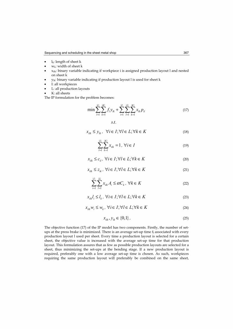
• xilk: binary variable indicating if workpiece i is assigned production layout l and nested on sheet k

• ylk: binary variable indicating if production layout l is used for sheet k

• I: all workpieces

• L: all production layouts

• K: all sheets The IP formulation for the problem becomes:

| | | | | | | | | |

1 1 1 1 1

minL K I L K

l lk lk il

l k i l k

f y x p= = = = =

+ (17)

. . s t

ilk lkx y≤ , ; ;i I l L k K∀ ∈ ∀ ∈ ∀ ∈ (18)

| | | |

1 1

1L K

ilk

l k

x= =

= , i I∀ ∈ (19)

ilk ilx c≤ , ; ;i I l L k K∀ ∈ ∀ ∈ ∀ ∈ (20)

ilk ikx z≤ , ; ;i I l L k K∀ ∈ ∀ ∈ ∀ ∈ (21)

| | | |

1 1

I L

ilk i k

i l

x A Cα= =

≤ , k K∀ ∈ (22)

ilk i kx l l≤ , ; ;i I l L k K∀ ∈ ∀ ∈ ∀ ∈ (23)

ilk i kx w w≤ , ; ;i I l L k K∀ ∈ ∀ ∈ ∀ ∈ (24)

, {0,1}ilk lkx y ∈ , (25)

The objective function (17) of the IP model has two components. Firstly, the number of set-ups at the press brake is minimized. There is an average set-up time fl associated with every production layout l used per sheet. Every time a production layout is selected for a certain sheet, the objective value is increased with the average set-up time for that production layout. This formulation assures that as few as possible production layouts are selected for a sheet, thus minimizing the set-ups at the bending stage. If a new production layout is required, preferably one with a low average set-up time is chosen. As such, workpieces requiring the same production layout will preferably be combined on the same sheet,


creating less set-ups at the press brake. Secondly, the total bending time at the press brake is minimized. A workpiece's bending time is influenced by the selected production layout for bending. The second part of the objective function assures that workpieces are assigned to a production layout with low bending times in order to decrease the makespan of the pool of jobs. Constraints (18) make sure that a workpiece can only be assigned to a specific production layout for a sheet, if that layout is selected for that particular sheet. The binary ylk variable will increase the objective function, every time a new production layout is required. Constraints (19) indicate that each workpiece should be produced, i.e. each workpiece should be assigned to a production layout and should be nested on a sheet for cutting. Constraints (20) limit the layouts that can be used for a certain workpiece. The binary workpiece-layout matrix indicates whether a certain workpiece i can be made with layout l. Not all workpieces can be produced with all available production layouts because of restrictions imposed by the workpiece’s geometry. Constraints (21) verify if a workpiece can be nested on a certain sheet, based on the material type and the sheet thickness. Constraints (22) guarantee that the total usable area (Ck) of a sheet is not exceeded while nesting the different workpieces. A safety zone ( ) is taken into account. This ( ) takes into account the required spacing between workpieces (heat build-up when cutting) and the clamping zone. Constraints (23) and (24) check the length and width of a workpiece compared to the length and width of a particular sheet to avoid creating infeasible nestings. Constraints (25) limit the decision variables to Boolean values. The result of the mathematical model (17-25) determines for each sheet which workpieces should be combined for cutting (nesting). It is important to note that the actual arrangement of those workpieces on the sheet is not generated by the IP model. Dedicated algorithms, implemented in commercial software, allow to generate the best arrangement, taking into account process planning aspects such as heat build up when cutting, piercing of initial holes, cutting path minimization etc. It is not the purpose of this research to introduce process planning issues in the production planning module. Besides the groupings of the workpieces, the IP model also indicates for each workpiece the required production layout for bending. The total number of production layouts is thus minimized and all workpieces are assigned to a unique production layout. Besides a possible makespan reduction (due to the reduced set-up time at the press brake), material utilization plays an important role. Minimization of the number of sheets is not as such included in the mathematical model. The number of sheets is fixed in advance (user-defined). This number can be determined based on:

• the theoretical number of sheets: for every material type and sheet thickness, the total parts' area is divided by a sheet's area and rounded upwards and the necessary margins for clamping, etc. are taken into account;

• the optimal number of sheets as determined by dedicated nesting software: commercial packages can be used to determine for each material type and thickness the amount of sheets required.

The exact production sequence for the different sheets is not determined by the IP model. Since the sheet metal shop is seen as a flow shop with single machines at each stage, the order of cutting the sheets also determines the order of bending the sheets and vice versa. In the presented research, the order of cutting the sheets is determined by the bending stage. This means that the sheets are sequenced such that the set-ups between production layouts of consecutive sheets at the press brake are minimized. It is important to notice that when


talking about the bend sequence, one usually discusses the sequence in which the bend

lines of an individual workpiece need to be executed to avoid collisions. For production planning issues, the bend sequence indicates the sequence in which the different sheets need to be bent. To avoid this confusion, a specific terminology has been developed:

• Bend sequence: is shown on the process plan and gives the sequence for producing the different bend lines of a workpiece (to avoid collisions when bending the workpiece, e.g. bend line 1 - bend line 5 - bend line 3 - etc. ).

• Production sequence: is related to the production plan and gives the sequence for cutting and bending the sheets (e.g. sheet 1 - sheet 4 - sheet 3). The term production sequence is used for flow shops with a single machine at each stage (the production sequence for cutting is then the production sequence for bending).

• Production bend sequence: is mentioned on the production plan and indicates for a sheet the sequence in which the different workpieces of that sheet need to be bent (e.g. workpiece 1 - workpiece 12 - workpiece 3).

The IP model neither generates the production sequence nor the production bend sequence for the different sheets. Thus, some additional steps are required to generate the final production plan. The list from the IP model indicates for each sheet the different workpieces to bend and the production layout to use. A TSP instance is solved for each sheet with the sequence-dependent set-ups between the production layouts as travel distances. The result of this step is a list with the different sheets, and the production bend sequence for bending the workpieces of each sheet. Next, a TSP instance is solved to determine the production sequence for the different sheets. In this last step, the sheets can swap/shift positions, but the production bend sequence of a sheet cannot be altered anymore. Table 6 displays a typical final production plan.

Demostuk (PL181) L_prof_1.5 (PL4) Banister_1.5 (PL66)

Voorbeeld (PL181) L_prof_1.5 (PL4) Banister_1.5 (PL66)

Schofbeurs (PL181) Banister_3 (PL66) Banister_1.5 (PL66)

Autodemo (PL25) Banister_3 (PL66) Banister_3 (PL66)

161757_test (PL25) Banister_3 (PL66)

Multifan (PL64) Banister_3 (PL66)

Banister_3 (PL66)

Cutting time (sec.) 223 394 594

Bending time (sec.) 1125 280 718

Set-up time (sec.) 372 376 0

Sheet1(S_1) Sheet2(SS_1.5) Sheet3(SS_1.5)

Table 6. Example of a final production plan

5.2.2 Computational experience

To verify the ability to generate qualitative integrated production plans, different real-life test cases are used. In total, 30 orders/jobs are included (complex workpieces and profiles). Two materials, i.e. steel (S) and stainless steel (SS) and five thicknesses ranging from 1mm to 6mm are included in the test batch. Based on the available tool segments in the test-case company, 201 different production layouts (PL) are selected.


The results of the production planning model are compared with the reference approach for that particular case. This reference approach can be interpreted as “the current way of planning”. For the reference approach, nesting is carried out with dedicated nesting software (CADMAN-PL) and for bending, the production layout is selected by an experienced operator. The IP-model (17-25; called Appr1) is generated in C++ and solved with ILOG CPLEX V10.01. Table 7 displays the results obtained.

Case

Thick_1mm 1.24 8.6 21.0 25.6 420.0 0.0

Thick_1.5mm 0.58 6.3 15.4 40.6 71.0 0.0

Thick_2mm 0.9 7.6 18.6 38.9 3.2 0.0

Thick_3mm 0.91 3.2 7.7 6.1 91.0 0.0

Thick_6mm 11.78 0.3 0.8 89.5 3600.0 36.9

Thick_small 0.78 3.7 8.9 44.7 131.7 0.0

Thick_small_profiles 0.54 4.6 11.3 42.3 10.1 0.0

Thick_small_complex 1.87 4.0 9.8 35.3 7.2 0.0

Thick_large_profiles 3.8 1.0 2.5 72.5 19.3 0.0

Thick_large_complex 11.11 0.6 1.4 42.3 3600.0 31.0

AVERAGE 4.0 9.7 43.8

RatioMR

(%)

MR

(days/yr)

STR

(%)

GT

(sec)

GAP

(%)

Table 7. Results of the mathematical model (Appr.1)

Material utilization: Compared to the reference approach, no additional sheets are required when the integrated planning model is used. Note that in the planning model the number of sheets is determined based on the theoretical minimal number of sheets (i.e. the total required area per thickness and material, taking into account some safety zones). This number is user-defined to set an upper limit to the number of different sheets. The main difference between the reference case and the integrated model is the arrangement of the nested workpieces and hence the geometry of the remnant sheets, i.e. sheets that are partially filled and stored for later use. The surface of the remnant sheets remains approximately the same since the total surface to nest is identical for both cases, but the geometry can be different due to the grouping of different workpieces. Note also that the actual layout of the sheets (the parts' positioning) is to be determined with dedicated nesting software. Process planning details such as cutting path, laser technology, lead-ins, piercings, etc. are also determined with this specialized software tool. Makespan reduction: On average a makespan reduction (MR) of about 4.1% is obtained for the complete batch of the ten cases. On daily basis one would be able to save 0.32 hours (almost 20 minutes). Extrapolating this to a complete year results in an average saving of approximately 11.3 working days if the batches would be continuously reproduced during the year. The makespan reduction is the highest for the instances that comprise mainly workpieces with small sheet thickness. This can be explained due to the fact that for small sheet thickness, the cutting and bending time are of comparable magnitude. Any reduction in the set-up time at the bending stage contributes to makespan reduction. If the sheet thickness increases, the laser time increases drastically. The bending time, however, does not increase accordingly. For large sheet thickness, cutting will thus require much more time compared to bending. The laser machine becomes dominant and reductions at the press brake are insignificant compared to the total production time. To determine the cases where one of the machines is dominant, the production times of both machines are compared. The ratio between the total cutting time and the total bending time should be calculated. If this

8.8

4.1 11.3


ratio is smaller than 0.5 or larger than 2, one of the machines is considered dominant. The ratios of the cases are mentioned in Table 7. As can be seen, if one of the machines is dominant, the integrated approach yields negligible makespan reductions. Set-up time reduction: Besides the reduced makespan, the set-up time at the bending stage decreases on average with 43.8% (STR: set-up time reduction). This can be explained by the fact that the mathematical model minimizes the number of production layouts to produce a batch of workpieces. A reduced number of production layouts results in a reduced set-up time at the press brake. The proposed approach analyzes the workpiece/layout matrix and produces if possible many workpieces with a common production layout. An experienced operator will try to do the same, but as the number of workpieces and/or production layouts increases, this becomes more difficult. Additionally, the different sheets are grouped in such a way that set-ups between subsequent sheets are avoided (TSP formulation). Generation time and quality of the solution: The model is run for 60 minutes maximum. If an optimal solution is not reached, the gap between the linear relaxation and the best solution found is mentioned. As can be observed, the optimal solution cannot be obtained within a reasonable amount of time in all cases. Another shortcoming of the approach is the use of sequence-independent set-up times between the different production layouts. To somewhat overcome this problem, a traveling salesperson formulation with sequence-dependent set-ups is applied to sequence the workpieces per sheet. Although the quality is improved by including this step, better solutions might be possible. The interested reader is referred to Verlinden et al. (2007).

5.3 Reformulation of the planning problem

5.3.1 Vehicle routing

The classical vehicle routing problem formulation (VRP) is a well-known integer programming problem which falls into the category of NP-Hard problems. The aim of solving VRPs is to design the optimal set of routes for a fleet of vehicles in order to serve a given set of customers. If the trucks have a limited capacity, the problem is a capacitated vehicle routing problem (CVRP). The (C)VRP can be seen as an “intersection” of two well-known combinatorial problems: the traveling salesperson problem (TSP) and the bin packing problem (BPP). A good overview of the VRP is given by (Laporte et al., 2000). When an integrated production plan needs to be generated for sheet metal laser cutting and bending, two main issues need to be tackled: 1. the workpieces need to be grouped on the sheets, minimizing the waste material; 2. the number of set-ups for bending needs to be minimized, taking into account

sequence-dependent set-ups between the production layouts at the press brake. It appears that the optimization task is a combination of bin packing (filling a minimal number of sheets) and set-up-time minimization (minimizing sequence-dependent set-ups at the press brake). Hence, an integrated sheet metal production planning can, after small modifications, be modeled as a VRP, more precisely as a CVRP due to the limited sheet capacity. The sheets with a limited usable sheet area represent the trucks with a limited and fixed capacity. The workpieces with a certain surface represent the different customers with a specific demand and the set-up times between the production layouts for bending represent the traveling distances between the different customers. It is important to note that there remain some differences between the standard CVRP and the integrated sheet metal production planning problem. The IP formulation of the CVRP


should thus be modified to address the problem. Yet, the CVRP formulation is a good starting point for modeling. Figure 12 gives a rough sketch of the reformulation.

Figure 12. Reformulating sheet metal production planning as a VRP instance (PL = production layout)

5.3.2 IP formulation

Following parameters and variables are used:

• i,j: workpiece indices

• k: sheet index

• sij: set-up time between the production layout of workpiece i and the production layout of workpiece j

• Ai: surface of workpiece i

• Ck: capacity of sheet k

• xijk: binary variable indicating if workpiece i is followed by workpiece j on sheet k

• I: all workpieces. Workpiece zero is the depot.

• K: all sheets The mathematical formulation of the alternative approach for sheet metal integrated production planning becomes:


| | | | | |

0 0 1

minI I K

ij ijk

i j k

s x= = =

(26)

. . s t

| | | |

1 1

1I K

ijk

j k

x= =

= , 0i I∀ ∈ (27)

| |

0

1

1I

jk

j

x=

= , k K∀ ∈ (28)

| |

0

1

1I

i k

i

x=

= , k K∀ ∈ (29)

| | | |

1 1

0I I

ihk hjk

i j

x x= =

− = , ;h I k K∀ ∈ ∀ ∈ (30)

| | | |

1 1

I I

i ijk k

i j

A x Cα= =

≤ . k K∀ ∈ (31)

( )i j ijk i j ijk ju u Qx Q A A x Q A− + + − − ≤ − , , ; ;i j I i j k K∀ ∈ ≠ ∀ ∈ (32)

i iA u Q≤ ≤ , i I∀ ∈ (33)

{0,1}ijkx ∈ (34)

The objective function (26) minimizes the total set-up time between the production layouts of the different workpieces. In this formulation sequence-dependent set-up times are used. A minimization of the number of sheets is not incorporated in the objective function. This number of sheets is preset to a user-defined fixed quantity, based on the theoretical minimum number of required sheets for that particular batch (K-value is fixed) or based on the number of sheets required by dedicated nesting software. If a feasible solution cannot be found with the preset quantity of sheets, the number of sheets (characterized by a specific material and thickness) is increased with one. Production constraints (27) make sure that every workpiece is included on a sheet and hence produced. Constraints (28) and (29) originate from the general (capacitated) vehicle routing problem: every truck must start and end at the depot. These constraints are needed to generate the production bend sequence for each sheet. Flow constraints (30) maintain the flow for a truck: if a truck enters a city, it will also leave that city. Translated to the sheet metal planning problem: if a workpiece is bent, it will be preceded and followed by another workpiece. This constraint creates per sheet a

j=0

j=0 i =0

i =0


smooth sequence for bending the different workpieces. Capacity constraints (31) ensure that a sheet is only filled to at most its available capacity (taking into account safety margins). Subtour elimination constraints (32) and (33) make sure that no infeasible flows of workpieces are created for bending. Constraints (34) limit the decision variables to Boolean values.The production sequence is not yet determined by applying this alternative approach. To sequence the different sheets, a TSP formulation is used. In this last step only the order of the sheets is altered because this might reduce the set-ups between consecutive sheets. To generate an integrated production plan for laser cutting and air bending with the CVRP-based approach (Appr.2), a number of steps need to be followed.

• All workpieces to be produced within T days are collected in a pool of jobs.

• Each workpiece is assigned a unique production layout by solving a simple plant location problem (SPLP) instance. This SPLP approach minimizes the number of different production layouts required to produce the pool of jobs. The interested reader is referred to Verlinden et al. (2007).

• An IP formulation (CVRP based) is solved to assign the different workpieces to sheets and to determine the production bend sequence for each sheet.

• A TSP instance is solved to determine the final production sequence (set-up time between production layouts of consecutive sheets will be minimized).


The results of this alternative approach (Appr.2) are compared against both the first approach (Appr.1) and the reference approach. Material utilization: Waste material minimization is all-persuasive in the sheet metal shop due to the ever increasing prices for the raw materials. To assure that the number of sheets is minimized, user-defined values are used, based on the amount of sheets required when nesting the parts with dedicated software tools. It appears that, in all cases, the integrated approach requires no additional sheets compared to the reference approach. Makespan reduction: As can be observed from Table 8, modeling the integrated sheet metal production planning problem as a modified CVRP instance results in an average makespan reduction of 5.1%. If the batches would be continuously reproduced, 13.4 working days could be saved on a yearly base, compared to the reference approach. Compared to the very first mathematical model, the average makespan reduction is higher (4.1 to 5.1%). In the alternative approach, sequence-dependent set-ups at the press brake are included in the objective function. This results in alternative groupings of workpieces as compared with the first model. Here again, as the amount of thicker workpieces increases, the makespan reduction decreases. Set-up time reduction: An average set-up time reduction of 48.8% can be observed for the different test cases. This extra time can be used for bending other workpieces or for performing administrative tasks, etc. Since experienced press brake operators are hard to find, any set-up time reduction at the press brake is very valuable for the companies. Generation time: Table 8 also displays the required generation time (GT) for the different test cases. Compared to the previously proposed IP model, more computational time is required to generate the solution. The quality of the solution is, however, better.


Case

Thick_1mm 1.24 8.6 10.9 26.7 45.0 420.0 932.4 0.0

Thick_1.5mm 0.58 6.3 7.3 17.7 44.9 71.0 83.0 0.0

Thick_2mm 0.90 7.6 8.2 19.9 41.8 3.2 16.4 0.0

Thick_3mm 0.91 3.2 4.7 11.4 6.1 91.0 321.7 0.0

Thick_6mm 11.78 0.3 0.3 0.8 90.5 3600.0 3600.0 41.0

Thick_small 0.78 3.7 4.2 10.2 45.2 131.7 412.0 0.0

Thick_small_profiles 0.54 4.6 6.1 14.6 52.0 10.1 317.0 0.0

Thick_small_complex 1.87 4.0 4.3 10.5 36.2 7.2 96.7 0.0

Thick_large_profiles 3.80 1.0 1.2 2.8 83.9 19.3 122.2 0.0

Thick_large_complex 11.11 0.6 1.0 2.4 42.3 3600.0 3600.0 36.0

AVERAGE 4.0 4.8 11.7 48.8

GT

Appr.2

(sec)

GAP

Appr.2

(%)

MR

Appr.2

(days/yr)

STR

Appr.2

(%)

GT

Appr.1

(sec)

Ratio

MR

Appr.1

(%)

MR

Appr.2

(%)

Table 8. Results of the second approach (Appr.2) compared to the reference approach and the first model (Appr.1)

Thus it can be concluded that modeling the integrated planning problem as a modified CVRP allows to generate good production plans. It reduces the makespan compared to the current way of planning. Compared to Appr.1, the makespan is more significantly reduced (since now sequence-dependent set-ups at the press brake are taken into account already at the nesting stage). Unfortunately, computational times are for some cases too large and between subsequent sheets sequence-independent set-ups are used. To tackle both issues, a variable neighborhood search heuristic is developed. This VNS procedure will allow to generate production plans of high quality almost instantaneously.

5.4 Variable neighborhood search

For the variable neighborhood procedure, a number of moves are defined. Swap_task swaps two tasks which may not be adjacent. With shift_task a task is removed from one position in the sequence and inserted at another position (either before or after the original position). Some problem instances contain a number of jobs, each consisting of a small number of similar tasks. Especially for this kind of problem, two additional neighborhood structures are defined. Swap_job swaps two jobs (each consisting of more than one task) which may not be adjacent. This swap is only considered when the two jobs are on the same sheet or when all tasks of the two jobs each are on a same sheet. With shift_job a job is removed from one position in the sequence and inserted at another position (either before or after the original position). Again, all the tasks of the job have to be on the same sheet. When the considered tasks or jobs are on different sheets, these four types of moves are only considered when the two sheets have the same thickness and are of the same material. Also, the total used surface of both sheets has to be smaller than the usable surface of a sheet. On this level, a fifth neighborhood shift_sheet can be defined. A move is executed by removing a sheet from one position in the sequence and inserting it after some other sheet. For this neighborhood the best position to insert a sheet is searched and this move is executed when it results in a better objective function value. Note that it is possible that the production layout for bending the last task on a sheet is the same as the one required by the first task on the next sheet. In that case shifting that sheet to another position in the sequence is probably not beneficial. Therefore, not only single sheets are considered for shifting but also subsequences of sheets where the last task of the previous sheet and the first task of the next sheet require the same production layout.

8.8 9.9 24

4.1 5.1 13.4


For the order in which a neighborhood is searched, a fixed natural lexicographic ordering, i.e. (1,2), (1,3), … (1,n), (2,1), (2,3), … , (i,j), …, (n-1,n) is used. For swap-moves only pairs where i<j are considered. Each time an improving move is executed, the next iteration continues with the same i and the next j value. The procedure applied to the different problem instances starts with a descent method with the swap_task neighborhood. On the resulting sequence, a descent method based on the shift_task neighborhood is applied. Then, the shift_sheet neighborhood is searched. Finally, the swap_job and shift_job neighborhoods are searched. When during one of these five descent procedures an improvement is found, the complete cycle with the five neighborhoods is repeated until no improvement can be found with one of the five neighborhoods. In this way, a local optimum relative to five different neighborhood structures is determined. Figure 13 displays the different neighborhoods. Another issue is the choice of the starting solution. The search is initialized with a first solution, constructed by grouping together tasks that require the same material and sheet thickness. Metal sheets are filled until no more workpieces can be added. Different orderings in which the tasks are grouped, can be considered: 1. as given in the problem data input (ordered by thickness); 2. the reverse order of the problem data input; 3. based on the tool layout number: from small to large; 4. calculated by the nearest neighbor heuristic: the first task is the one with the smallest

average set-up time; following tasks are added by looking for the smallest set-up time from the actual task to the following task.

By using these four initial seeds, a multi-start approach is implemented.

Figure 13. Different neighborhood structures in the VNS procedure



The same ten test-cases have been applied. The generation time for the VNS procedure is for all test cases less than one second. Table 9 indicates that the makespan and set-up time are reduced as compared to both the first and second mathematical model.

Case

Thick_1mm 8.6 10.9 11.1 25.6 45.0 44.0

Thick_1.5mm 6.3 7.3 7.3 40.6 44.9 45.0

Thick_2mm 7.6 8.2 8.2 38.9 41.8 41.0

Thick_3mm 3.2 4.7 5.6 6.1 6.1 6.0

Thick_6mm 0.3 0.3 0.5 89.5 90.5 90.0

Thick_small 3.7 4.2 4.4 44.7 45.2 51.6

Thick_small_profiles 4.6 6.1 6.3 42.3 52.0 52.0

Thick_small_complex 4.0 4.3 7.8 35.3 36.2 45.0

Thick_large_profiles 1.0 1.2 1.5 72.5 83.9 85.0

Thick_large_complex 0.6 1.0 1.3 42.3 42.3 47.5

AVERAGE 4.0 4.8 5.4 43.8 48.8 50.7

MR

VNS

(%)

STR

Appr.1

(%)

STR

Appr.2

(%)

STR

VNS

(%)

MR

Appr.1

(%)

MR

Appr.2

(%)

Table 9. Comparison of the results

5.5 Summary

To overcome the problems due to separate optimization of the cutting and bending process, integrated production planning models are proposed. An IP model allows to generate integrated production plans, but the use of sequence independent set-ups at the bending stage decreases the solution quality. A second formulation (a modified CVRP instance) includes sequence dependent set-ups and hence increases the solution quality, but computational times are still too large. A variable neighborhood search procedure is developed to generate production plans of high quality in an acceptable time frame. The makespan reduction is the largest in those cases where the cutting and bending operation are somewhat balanced, i.e. the production times are of comparable magnitude. If one of the operation stages is clearly dominant, the makespan reduction is negligible. The set-ups at the press brake are in all cases (balanced or not) reduced.

6. Conclusions and future research

Although process planning issues for sheet metal operations are largely computerized, production planning is still carried out by hand and is based on human experience. This chapter addressed the authors' effort to computerize and optimize different sheet metal production planning issues. Specific models of a combinatorial nature and dedicated algorithms were developed by the authors to design efficient production plans. A first problem is the layout outline for the placing of the different stations on a press brake, minimizing the travel distance for the press brake operator. The proposed approach takes asymmetric deformations, due to the use of long stations, into account and generates good solutions. The use of a local search procedure assures that solutions are generated in a short period. The developed algorithms are implemented in commercial CAD software tools,

8.8 9.9 9.9

4.1 5.1 5.6


allowing to generate automatically and instantaneously the required production layout when designing a sheet metal part. The generated production layouts are then used in an automated procedure to determine the production plan for sheet metal air bending. The proposed algorithms minimize the makespan of the pool of jobs by reformulating the planning problem as a TPP or GTSP. The results indicate that production planning for air bending can indeed be automated and good results can be obtained compared to production plans generated by an experienced operator. In this context also (guided) local search techniques are used to generate solutions of good quality in a short period. This is very important since the generation of a production plan should be done almost instantaneously at distinct moments. Research on sheet metal production planning revealed that it is mandatory to look at the entire sheet metal production chain when generating production plans. If the distinct production plans are sequentially combined, only a sub-optimal plan is achieved for the shop. Procedures are proposed for integrating laser cutting with air bending. The different algorithms allow to approach the problem in an integrated way, resulting in reduced set-up times at the press brake and a reduced makespan for the pool of orders. The results reveal that, although considered very difficult by many, sheet metal production planning can indeed be automated at least for relatively simple configurations (flow shop with single machines at the two stages). As a result, significant improvements are obtained compared to current planning practices. Ongoing research focuses on the inclusion of multiple machines at both the cutting stage and bending stage. At the different stages, multiple machines with different characteristics are available. An additional task is now to assign the sheets to the different machines, still minimizing the makespan. Future research will address the challenge to include other processes such as welding, painting packaging etc. The main objective will however not change: generating integrated production plans with a reduced makespan in a very short time period.

7. Acknowledgment

The authors acknowledge the financial support from IWT-Vlaanderen (Instituut voor de Aanmoediging van Innovatie door Wetenschap en Technologie Vlaanderen).

8. References

Adamowicz, M. & Albano, A. (1976). A solution to the rectangular cutting-stock problem. IEEE Transactions on System Science and Cybernetics, 6, pp. 302–310

Crauwels, H.; Collin, P.; Duflou, J. & Van Oudheusden, D. (2005). Tooling layout on a press brake for sheet metal air bending. Production Planning & Control, 16(5), pp. 514-525

El-Darzi, E. & Mitra, G. (1995). Graph theoretic relaxations of set covering and set partitioning problems. European Journal of Operations Research, 87, pp. 109-121

Duflou, J.R.. (1999). Automatic design verification and process planning for bent sheet metal parts. PhD dissertation, ISBN: 90-5682-190-3, Katholieke Universiteit Leuven, Belgium


Duflou, J.R. ; Nguyen, T.H.M. ; Kruth, J.-P. & Cattrysse, D. (2003). An optimization system for automated workpiece layout generation for bent sheet metal parts. Proceedings of the 10th international conference on sheet metal, pp. 235-244, ISBN: 1-85923-171-3, Belfast, April 2003

Duflou, J.R.; Vancza, J.; & Aerens, R. (2005). Computer aided process planning for sheet metal bending: a state of the art. Computers in Industry, 56, pp.747–771

Eisemann, K. (1957). The trim problem. Management Science, 3, pp. 279–284 Erlenkotter, D. (1978). A dual-based procedure for uncapacitated facility location, Operations

Research, 26, pp. 992–1009 Fries-Knoblach, J. Sheet metalworking in the bronze age and iron age in southern central

Europe. (1999). Proceedings of the 7th international conference on sheet metal, pp. 23-34, ISBN: 3-87525-110-5, Erlangen, September 1999

Herrman, J. & Delalio, D. (1998). Evaluating sheet metal nesting decisions. Technical report,Institute for systems research

Haessler, R.W. & Sweeney, P.E. (1991). Cutting stock problems and solution procedures. European Journal of Operational Research, 54(2), pp. 141-150

Johnson, D.S. & McGeoch, L.A. (1997). The traveling salesman problem: a case study. Combinatorial Optimization, pp.215-310, Wiley: Chisester-UK

Kara, I.; Laporte, G. & Bektas, T. (2004). A note on the lifted miller tucker zemlin sub tour elimination constraints for the capacitated vehicle routing problem. EuropeanJournal of Operational Research, 158(3), pp. 793–795

Kreher, D.L. & Stinson, D.R. (1999). Combinatorial algorithms: generation, enumeration and search. CRC Press, ISBN 9780849339882, Boca Raton

Laporte, G.; Gendreau, M.; Potvin, J.Y. & Semet, F. (2000). Classical and modern heuristics for the vehicle routing problem. International Transactions in Operational Research, 7, pp. 285–300

Lee, H.C. & Woo, T.C. (1988). Determining in linear time the maximum area convex hull of two polygons. IEEE Transactions, 20(4), pp. 338-345

Lo Valvo, E. & Licari, R. (2007). A more efficient method for clustering sheet metal shapes. Key engineering materials, 344, pp.921-927

Mladenovi , M. & Hansen, P. (1997). Variable neighborhood search. Computers & Operations Research, 24(11), pp. 1097–1100

Nguyen, T.H.M. (2005). Automatic tool selection and dimensional accuracy verification in computer aided process planning for sheet metal bending. PhD dissertation, ISBN 90-5682-647-3, Katholieke Universiteit Leuven, Belgium

Nye, T.J. (2001). Optimal nesting of irregular convex blanks in strips via an exact algorithm. International journal of Machine tools & Manufacture, 41, pp. 991–1002

Pearn, W.L. (1991). On the traveling purchaser problem. Working paper 91-01, National Chiao Tung University.

Prasad, Y.K.D.V. (1994). A set of heuristic algorithms for optimal nesting of two-dimensional irregularly shaped sheet metal blanks. International Journal of Production Research, 33, pp. 1505 - 1520

Ramesh, R. (1981). Traveling purchaser problem. Opsearch, 18, pp. 78-91 Singh, K.N. & Van Oudheusden, D. (1997). A branch and bound algorithm for the traveling

purchaser problem. European Journal of Operations Research, 97, pp. 571-579


Srivastava, S.S.; Kumar, S.S.; Carg, R.C. & Sen, P. (1969). Generalized traveling salesperson problem through n sets of nodes. Journal of the Canadian Operations Research Society,7, pp. 97-101

Tang, C.H. & Rajesham, S. (1994). Computer aided nesting in sheet metal for press working operations involving bending. Journal of Material processing Technology, 44(3-4), pp. 319-326

Vansteenwegen, P. & Gheysens, J. (2002). Bewegingsanalyse en tijdsraming voor buigprocessen. Master’s thesis, Katholieke Universiteit Leuven, Belgium

Verlinden, B., Cattrysse, D. & Van Oudheusden, D. (2007) Integrated sheet metal production planning for laser cutting and air bending. Proceedings of the International Conference on Competitive Manufacturing, pp. 425-431, Stellenbosch - South Africa, January 2007

Voudouris, C. & Tsang, E. (1999). Guided local search and its application to the traveling salesperson problem. European Journal of Operational Research, 113, pp. 469–499

Multiprocessor Scheduling, Theory and ApplicationsEdited by Eugene Levner

ISBN 978-3-902613-02-8Hard cover, 436 pagesPublisher I-Tech Education and PublishingPublished online 01, December, 2007Published in print edition December, 2007

InTech EuropeUniversity Campus STeP Ri Slavka Krautzeka 83/A 51000 Rijeka, Croatia Phone: +385 (51) 770 447 Fax: +385 (51) 686 166www.intechopen.com

InTech ChinaUnit 405, Office Block, Hotel Equatorial Shanghai No.65, Yan An Road (West), Shanghai, 200040, China

Phone: +86-21-62489820 Fax: +86-21-62489821

A major goal of the book is to continue a good tradition - to bring together reputable researchers from differentcountries in order to provide a comprehensive coverage of advanced and modern topics in scheduling not yetreflected by other books. The virtual consortium of the authors has been created by using electronicexchanges; it comprises 50 authors from 18 different countries who have submitted 23 contributions to thiscollective product. In this sense, the volume can be added to a bookshelf with similar collective publications inscheduling, started by Coffman (1976) and successfully continued by Chretienne et al. (1995), Gutin andPunnen (2002), and Leung (2004). This volume contains four major parts that cover the following directions:the state of the art in theory and algorithms for classical and non-standard scheduling problems; new exactoptimization algorithms, approximation algorithms with performance guarantees, heuristics and metaheuristics;novel models and approaches to scheduling; and, last but least, several real-life applications and case studies.

How to referenceIn order to correctly reference this scholarly work, feel free to copy and paste the following:

B. Verlinden, D. Cattrysse, H. Crauwels, J. Duflou and D. Van Oudheusden (2007). Sequencing andScheduling in the Sheet Metal Shop, Multiprocessor Scheduling, Theory and Applications, Eugene Levner(Ed.), ISBN: 978-3-902613-02-8, InTech, Available from:http://www.intechopen.com/books/multiprocessor_scheduling_theory_and_applications/sequencing_and_scheduling_in_the_sheet_metal_shop

Documents

Sequencing and scheduling in the sheet metal shopcdn.intechweb.org/pdfs/629.pdf · Sequencing and scheduling in the sheet metal shop ... a punch press or cut with a laser machine