SERVIR Africa Workshop

Assessing the Vulnerability of Biodiversity to Climate Change

Report on the vulnerability of East African biodiversity to climate

change: Integrating the knowledge base on VETERBRATES

Report of Phase I activities

February 2012

Collaborative partnership with Yale University

Walter Jetz (PI)

Students and postdoc team members:

Katherine Mertes, Dr. Frank La Sorte, Dr. Morgane Barbet-Massin

AFRICAN CONSERVATION CENTRE

P O BOX 15289, 00509 Nairobi, KENYA

With kind support of:

2

Outline

I. Background and rationale

A. Global significance of East African biodiversity

B. Limited availability of species occurrence data for East Africa

C. Threats to East African biodiversity from climate change

II. Approach and methods

A. Expert range maps

B. Refined range maps

C. High-resolution range maps

D. Integrated model-based species distributions

E. Preliminary species distribution predictions under climate change

III. Phase I results

A. Expert range maps

B. Refined range maps

C. High-resolution range maps

D. Preliminary predictions of species richness under climate change

IV. Phase II proposed research

A. Minimizing uncertainty in high-resolution species distribution models

B. Assessing East African reserve networks under climate change

I. Background and rationale

A. Global significance of East African biodiversity

The geographic region of East Africa, comprising the countries of Kenya, Tanzania,

Uganda, Burundi, and Rwanda, contains an extraordinary variety of terrestrial vertebrate

diversity distributed across a land area of roughly 1.7 million km2. The region’s vegetation

communities, including deciduous and tropical forests, mangroves, savannas, open

grasslands, shrublands, and semi-desert areas, are highly heterogeneous, distinguished by

seasonal variation, soil composition, and precipitation and elevation gradients (Lehouerou

and Hoste 1977). Of particular ecological interest are its coastal and montane forests,

savannas, and numerous hotspots of endemism (Myers et al. 2000; Langhammer et al. 2007).

Past efforts to identify species distribution and richness patterns in East Africa have

generally focused on specific sub-regions, notably the Eastern Arc mountains (Burgess et al.

1998, 2007a), the Albertine Rift (Plumptre et al. 2007a), and the Serengeti and Maasai Mara

systems (Anderson et al. 2007). Repeated assessments have identified the Eastern Arc

Mountains, spanning Kenya and Tanzania and including the East Usambara and Udzungwa

blocs, as one of the most important areas in Africa for range-restricted vertebrate species and

endemic plants (Myers et al. 2000; Brooks et al. 2001). In a recent assessment of Eastern

Arc forests, however, Tabor et al. (2010) found an 11% reduction in forest area between

1970 and 2000, and described remaining forests as isolated fragments of 5 km2 or less

embedded in a matrix of degraded woodland and shrubland. Most forest loss has been

3

attributed to conversion for agricultural uses, timber extraction, and charcoal (Burgess et al.

2000). Eastern Arc forests are further threatened by road development and improvements,

and associated increases in accessibility (Prins and Clarke 2006).

Similarly, the Albertine Rift sub-region contains important centers of plant and vertebrate

endemism, as well as extremely high species richness and biomass (Brooks et al. 2001;

Plumptre et al. 2007b; Jefferson et al. 2008). The Albertine Rift encompasses much of the

Western Rift Valley in Tanzania, Uganda, Rwanda, and Burundi, and contains varied

ecosystems including wetlands, montane and lowland forest, and multiple types of savanna

(Plumptre et al. 2007a). While several transboundary initiatives are working to minimize

bushmeat hunting and animal trafficking in threatened species (Plumptre et al. 2007b), severe

threats to biodiversity conservation persist within this sub-region.

Finally, the Serengeti and Masai Mara, an area of approximately 25,000 km2 extending

from northwestern Tanzania into southern Kenya and defined by the migratory paths of

wildebeest (Connochaetes taurinus) between wet and dry seasons (Pennycuick 1975;

McNaughton 1985), is widely acknowledged as a globally unique landscape. Recent

assessments estimate that nearly 50% of the Serengeti-Mara system has been modified by

agricultural land uses, poaching, and additional pressures from increased human density

adjacent to protected areas (Homewood et al. 2001; Sinclair et al. 2007).

B. Limited availability of biodiversity data for East Africa

Despite the global significance of its biodiversity, little is known about the factors that

determine East African species distributions (Collen et al. 2008). Of the relatively few

studies of distribution patterns in the region, most emphasized select national parks (see, e.g.,

Western 1975), charismatic large vertebrates (McNaughton et al. 1988; Willlams et al. 2000),

or avian species (Crowe and Crowe 1982; Williams et al. 1999; Jetz and Rahbek 2001; De

Klerk et al. 2002a, b; Dillon and Fjeldsa 2005; McPherson and Jetz 2007; Romdal and

Rahbek 2009). The study of bird distributions has perhaps the longest history in the East

Africa, beginning with descriptive accounts (e.g. Chapin 1923) and continuing with statistical

and comparative analyses of avifaunal zones (Crowe and Crowe 1982; Williams et al. 1999;

De Klerk et al. 2002a; Romdal and Rahbek 2009).

Even when constrained to such geographic or taxonomic limits, studies of East African

species distributions have encountered substantial data limitations. Indeed, tropical areas

important for biodiversity conservation frequently lack readily available sources of

comprehensive data (Rahbek and Graves 2001; Ferrier 2002; Kuper et al. 2006). Common

obstacles to collecting and publicizing distribution data include insufficient funding, lack of

adequate infrastructure and expertise, and inaccessibility of sites for political or practical

reasons (Collen et al. 2008). For East Africa in particular, one previous analysis suggested

that much of the occurrence data from sub-Saharan Africa may be geographically biased

towards human habitation and transportation infrastructure (Reddy and Davalos 2003).

C. Threats to East African biodiversity from climate change

The Fourth Assessment (AR4) of the Intergovernmental Panel on Climate Change (IPCC

2007) provided further evidence of contemporary climate change, including strong warming

4

trends, altered precipitation patterns, accelerated melting of ice caps, and sea level changes

(IPCC 2007). In the region of sub-Saharan Africa, emerging and projected climate change

impacts include decreased precipitation, increases in drought-affected and arid lands, and

decreased yields from rain-fed agriculture (IPCC 2007). Due to this wide range of projected

impacts, as well as its low latitude and low adaptive capacity, the AR4 identified sub-Saharan

Africa as an area facing particularly high risks from climate change.

As climate change accelerates over the coming century, its consequences for biodiversity,

especially geographic shifts in species ranges (Thomas and Lennon 1999; Parmesan and

Yohe 2003; Root et al. 2003), temporal shifts in seasonal dynamics (Walther et al. 2002), and

species extinctions (McLaughlin et al. 2002), will increase in frequency. Because species

exhibit intrinsic differences in resource processing, engagement in ecological interactions,

and interaction strengths (Chapin et al. 1997; Chapin et al. 2000; McLaughlin et al. 2002)

these extinctions and altered distribution patterns will affect ecological processes and

ecosystem functions (Tilman et al. 1997; Emmerson et al. 2005, Wright et al. 2006),

potentially affecting sources of clean water, high-quality food, and commercial resources.

Climate change impacts to biodiversity will also likely affect tourism focused on wildlife and

natural landscapes, which contributes more than three billion USD in revenue to East African

countries (WTO 2006).

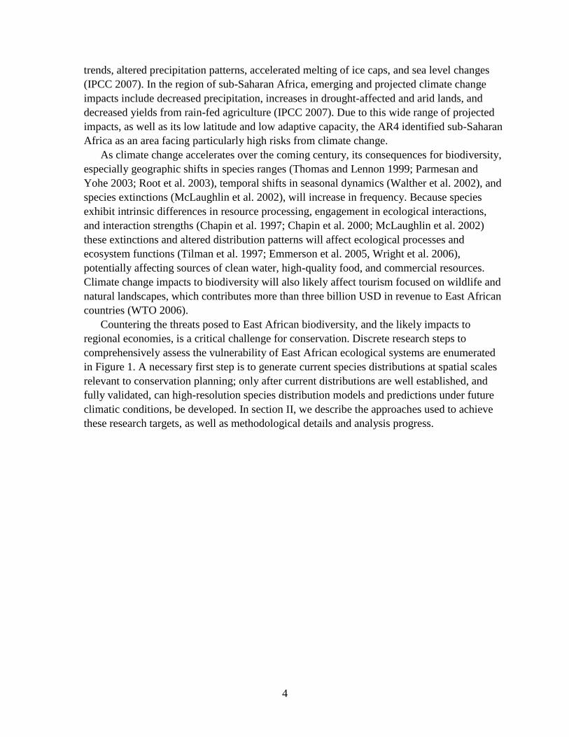
Countering the threats posed to East African biodiversity, and the likely impacts to

regional economies, is a critical challenge for conservation. Discrete research steps to

comprehensively assess the vulnerability of East African ecological systems are enumerated

in Figure 1. A necessary first step is to generate current species distributions at spatial scales

relevant to conservation planning; only after current distributions are well established, and

fully validated, can high-resolution species distribution models and predictions under future

climatic conditions, be developed. In section II, we describe the approaches used to achieve

these research targets, as well as methodological details and analysis progress.

5

Figure 1. Research targets for assessing vulnerability of East African vertebrate species to

climate change.

II. Approach and methods

A. Expert range maps

As a result of the limited biodiversity data available for East Africa, most previous

studies of regional biodiversity have been conducted at coarse spatial scales, such as 1x1-

degree grid cells, or approximately 110x110km (Burgess et al. 1998; Brooks et al. 2001;

de Klerk et al. 2002; McPherson and Jetz 2007). Coarse-scale assessments of species

richness have proven extremely useful in identifying the factors related to broad

dynamics of species distributions, such as evolutionary history, environmental conditions,

dispersal limitations, and energetics (Jetz and Rahbek 2002; Hawkins et al. 2003; Currie

et al. 2004; Hortal et al. 2008).

To generate a coarse-scale baseline of current East African species distribution

patterns, we compiled expert range maps, accurate for all species of amphibians, reptiles,

birds, and mammals that occur in East Africa (Spawls et al. 2004; Jetz et al. 2007; IUCN

2009) into a GIS database using ArcInfo version 10 (ESRI, Redlands, California, USA).

B. Refined range maps

While total spatial extent of species’ geographic ranges is often required for broad-

scale analyses and decision-making – such as IUCN threat category assignment – species

I. Expert range maps~ 100km resolution

II. Refined range maps~ 25km resolution

IV. Integrated model-based distributions

(combining all points, checklists, refined range maps)

25, 10, 1km resolution

III. Refined range maps~ 1km resolution

montane specialists

Status Projections

Complete(~ 2600 species)

Complete(~ 2600 species)

Empirical basis

Partially Complete

(montane birds: 105)

Change in distribution

Exposure

Change in distribution

ExposureP

has

e I

I

Inference, Value• Very limited• Grain too coarse to

be ecologically sound, useful for conservation

Ph

ase

I

Change in distribution

Exposure

• Useful for first prioritization of species, baseline assessment

• Very strong inference about extinction risk

• But only for few montane species

Effort

+

++

++

++++

Data gathering: ~ 1/4 complete

Methods: ~ 1/3 complete

• Best-possible inference of today’s and future distribution, species extinction risk

• Several critical assumptions remain

6

are not homogenously distributed across their range (Gaston and Fuller 2009). Within the

boundaries of a species’ range, many different habitat types and environmental conditions

likely occur, not all of which are suitable for the persistence of individual populations.

Coarse-scale estimates of a species' ranges are thus likely to overestimate species’

geographic distributions, and especially the probability that a species occurs at any one

site (Rondinini et al. 2005, Rondinini et al. 2006, Jetz et al. 2008). Precise mapping of the

area within range boundaries that is physically occupied by the species requires extensive

fine-grain occurrence data, typically collected through expensive and time-consuming

field surveys. Such data and sampling effort are not available for all species, or all

geographic regions – hence coarse-grain ranges remain widely used in studies of species

distribution, and will likely remain so for some time (Rodrigues et al. 2004).

Despite the dearth of fine-grain species occurrence data, much information is

available (for example, from the ecological literature and natural history publications)

about species-specific habitat and elevation preferences. These two pieces of information

provide categorical and numerical rules for species’ occurrence, which can be used to

refine coarse-scale ranges to only those areas likely to be inhabited by the species (see

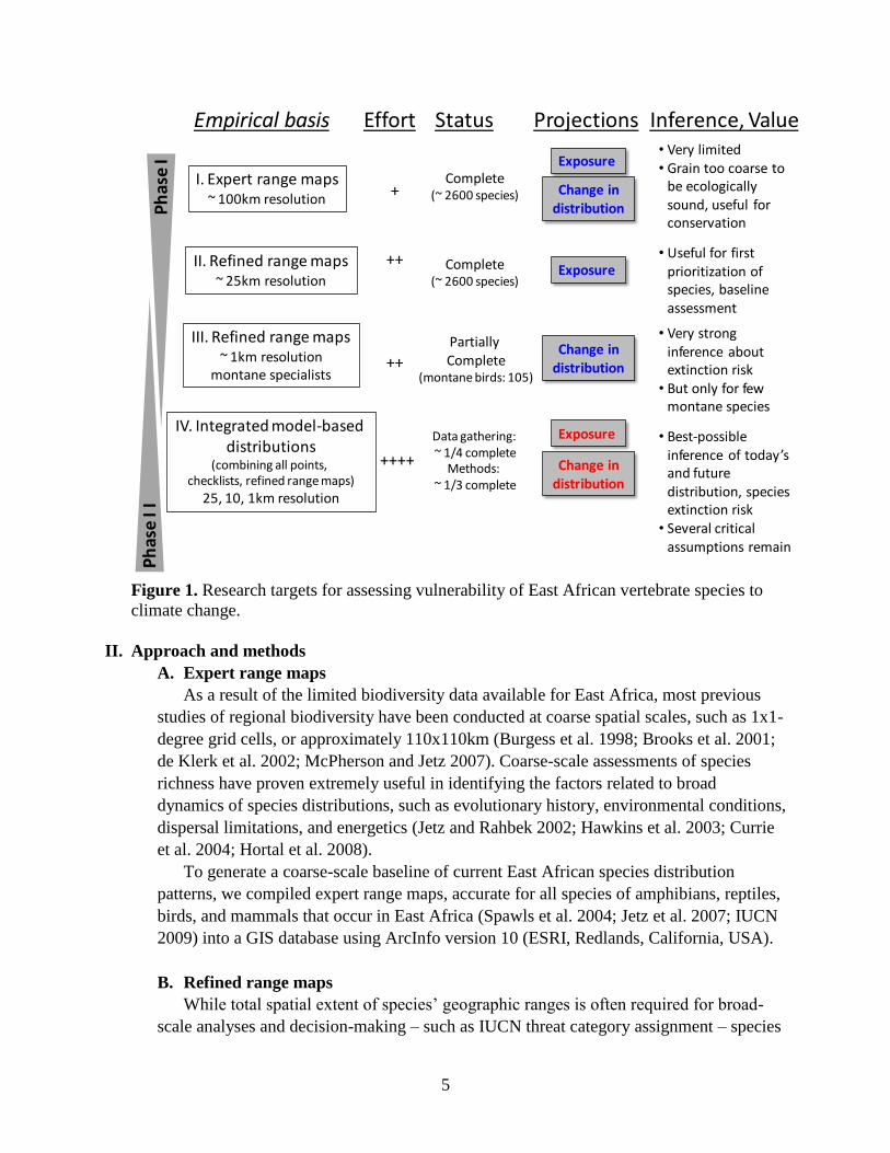
Scott et al. 2002). We compiled species-specific habitat and elevation preferences from

multiple sources (Perlo 1995; Spawls et al. 2004; Channing and Howell 2006; IUCN

Habitats Classification Scheme 3.0) and linked habitat descriptions with Globcover

global land cover map (ESA 2009) land cover classes, and elevational ranges with Shuttle

Radar Topography Mission (SRTM) topographical data (USGS 2004). All grid cells

within a species’ range containing unsuitable habitat or elevations were then eliminated

from the original range (Figure 2).

Figure 2. Species distribution of Hartlaub’s turaco (Turaco hartlaubi), with expert opinion range

in gray, suitable land cover in orange, and suitable land cover and elevation in green.

This range refinement was performed at a spatial scale of 300m due to the spatial

resolution of the Globcover land cover map (ESA 2009). While the refined species

distributions are likely accurate at a somewhat finer scale than the expert range, a

7

comprehensive validation process (see below) must be conducted before they may be

confidently used at for finer-grain research and planning processes.

C. High-resolution range maps

An increasing body of research suggests that some ecological processes important in

structuring species distributions, for example disturbance processes, biotic interactions,

and habitat selection, operate primarily at fine spatial scales (Shmida and Wilson 1985;

Whittaker et al. 2001; Ricklefs 2004; Hortal et al. 2008). Analyzing species distribution

data only accurate at coarse spatial grains thus risks overlooking the effects of fine-scale

processes, or conflating their influence with that of with coarse-scale factors (Rahbek and

Graves 2000; White and Hurlbert 2010).

This risk is readily illustrated in East African savanna systems. At the relatively

coarse scale of 0.5° grid cells, savanna vegetation may appear largely homogenous.

However, high-resolution satellite imagery or 1-10m2 survey plots reveal substantial

variation in abundance of grass and woody vegetation, caused by disturbance dynamics,

such as fire and grazing by livestock and native herbivores (Price et al. 2009). This

heterogeneity is highly relevant for local species, especially herpetofauna and small

mammals, because it occurs at a spatial scale more congruent with the scale at which

organisms perceive and interact with the environment (Fahr and Kalko 2010).

In the conservation planning context, such a scale “mismatch” could have highly

adverse consequences. For example, species distribution analyses limited to coarse spatial

scales may inadequately describe habitat and other resources for particular species. In one

study, the large-bodied skink Ctenotus robustus, known to prefer moderate to high

ground cover and related thermal conditions, was surprisingly abundant in open

woodland landscapes (Price et al. 2010). Investigation at a finer spatial grain found

numerous microsites suitable for C. robustus, suggesting that vegetation heterogeneity

undetectable at the landscape level was sufficient to support a viable population (Price et

al. 2010). In addition, fine-scale studies identify local threats, land use conflicts, and

other site-specific dynamics, providing specificity and precision for conservation actions

(Rouget 2003; Fjeldsa 2007). In sum, fine-grain analyses may both document an

ecological pattern and suggest its underlying mechanism, and thus offer eminently useful

information for conservation efforts.

In order to meet the demonstrated need for appropriately scaled species distribution

products, we compiled species occurrence data from sources including journal articles,

reports, book chapters, data portals such as the Global Biodiversity Information Facility

(GBIF), and natural history collections, especially those at the National Museums of

Kenya (NMK). Information about plant and animal specimens held at natural history

institutions is increasingly available to researchers via online data warehouses like GBIF

(Graham et al. 2004). However, substantial processing is typically required to translate

this information into high-quality – and high spatial resolution – species occurrence data

(Graham et al. 2004; Soberon and Peterson 2004; Guralnick and Hill 2009).

As an example, though expert staff may accurately identify specimens at the time of

accession, rapidly changing taxonomic conventions may render these identifications

8

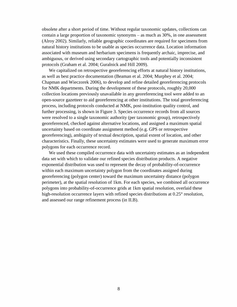
obsolete after a short period of time. Without regular taxonomic updates, collections can

contain a large proportion of taxonomic synonyms – as much as 30%, in one assessment

(Alroy 2002). Similarly, reliable geographic coordinates are required for specimens from

natural history institutions to be usable as species occurrence data. Location information

associated with museum and herbarium specimens is frequently archaic, imprecise, and

ambiguous, or derived using secondary cartographic tools and potentially inconsistent

protocols (Graham et al. 2004; Guralnick and Hill 2009).

We capitalized on retrospective georeferencing efforts at natural history institutions,

as well as best practice documentation (Beaman et al. 2004; Murphey et al. 2004;

Chapman and Wieczorek 2006), to develop and refine detailed georeferencing protocols

for NMK departments. During the development of these protocols, roughly 20,000

collection locations previously unavailable in any georeferencing tool were added to an

open-source gazetteer to aid georeferencing at other institutions. The total georeferencing

process, including protocols conducted at NMK, post-institution quality control, and

further processing, is shown in Figure 3. Species occurrence records from all sources

were resolved to a single taxonomic authority (per taxonomic group), retrospectively

georeferenced, checked against alternative locations, and assigned a maximum spatial

uncertainty based on coordinate assignment method (e.g. GPS or retrospective

georeferencing), ambiguity of textual description, spatial extent of location, and other

characteristics. Finally, these uncertainty estimates were used to generate maximum error

polygons for each occurrence record.

We used these compiled occurrence data with uncertainty estimates as an independent

data set with which to validate our refined species distribution products. A negative

exponential distribution was used to represent the decay of probability-of-occurrence

within each maximum uncertainty polygon from the coordinates assigned during

georeferencing (polygon center) toward the maximum uncertainty distance (polygon

perimeter), at the spatial resolution of 1km. For each species, we combined all occurrence

polygons into probability-of-occurrence grids at 1km spatial resolution, overlaid these

high-resolution occurrence layers with refined species distributions at 0.25° resolution,

and assessed our range refinement process (in II.B).

9

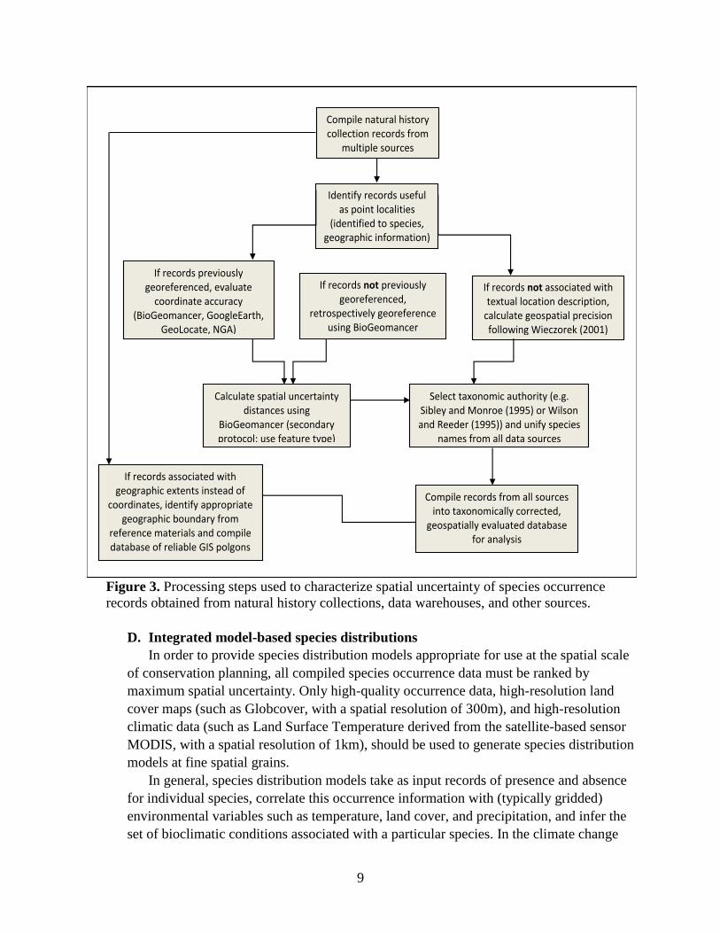
Figure 3. Processing steps used to characterize spatial uncertainty of species occurrence

records obtained from natural history collections, data warehouses, and other sources.

D. Integrated model-based species distributions

In order to provide species distribution models appropriate for use at the spatial scale

of conservation planning, all compiled species occurrence data must be ranked by

maximum spatial uncertainty. Only high-quality occurrence data, high-resolution land

cover maps (such as Globcover, with a spatial resolution of 300m), and high-resolution

climatic data (such as Land Surface Temperature derived from the satellite-based sensor

MODIS, with a spatial resolution of 1km), should be used to generate species distribution

models at fine spatial grains.

In general, species distribution models take as input records of presence and absence

for individual species, correlate this occurrence information with (typically gridded)

environmental variables such as temperature, land cover, and precipitation, and infer the

set of bioclimatic conditions associated with a particular species. In the climate change

If records previously georeferenced, evaluate

coordinate accuracy (BioGeomancer, GoogleEarth,

GeoLocate, NGA)

If records not previously georeferenced,

retrospectively georeference using BioGeomancer

If records not associated with textual location description,

calculate geospatial precision following Wieczorek (2001)

Compile natural history collection records from

multiple sources

Identify records useful as point localities

(identified to species, geographic information)

Compile records from all sources into taxonomically corrected,

geospatially evaluated database for analysis

If records associated with geographic extents instead of

coordinates, identify appropriate geographic boundary from

reference materials and compile database of reliable GIS polgons

Calculate spatial uncertainty distances using

BioGeomancer (secondary protocol: use feature type)

Select taxonomic authority (e.g. Sibley and Monroe (1995) or Wilson and Reeder (1995)) and unify species

names from all data sources

10

context, species distribution models can predict future distributions based on where each

species’ preferred environmental conditions are projected to occur under climate change.

As part of our Phase II activities, we will use the species occurrence data compiled during

Phase I to generate high-resolution models of both current and future distributions for all

terrestrial vertebrate species that occur in East Africa (see proposed modeling process in

Figure 5).

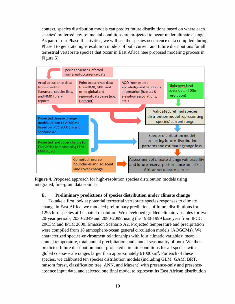
Figure 4. Proposed approach for high-resolution species distribution models using

integrated, fine-grain data sources.

E. Preliminary predictions of species distribution under climate change

To take a first look at potential terrestrial vertebrate species responses to climate

change in East Africa, we modeled preliminary predictions of future distributions for

1295 bird species at 1° spatial resolution. We developed gridded climate variables for two

20-year periods, 2030-2049 and 2080-2099, using the 1980-1999 base year from IPCC

20C3M and IPCC 2000, Emission Scenario A2. Projected temperature and precipitation

were compiled from 18 atmosphere-ocean general circulation models (AOGCMs). We

characterized species-environment relationships with four climatic variables: mean

annual temperature, total annual precipitation, and annual seasonality of both. We then

predicted future distribution under projected climatic conditions for all species with

global coarse-scale ranges larger than approximately 61000km2. For each of these

species, we calibrated ten species distribution models (including GLM, GAM, BRT,

ransom forest, classification tree, ANN, and Maxent) with presence-only and presence-

absence input data, and selected one final model to represent its East African distribution

11

under climate change.

For some species, climate change is likely to shrink the habitable climate space within

dispersal constraints or movement limits, potentially leading to substantial range

contractions. Montane species, in particular, will be forced towards higher elevations, but

may not always be able to shift their range upwards (Figure 4).

Figure 5. Constrained (A) and unconstrained (B) vertical dispersal in montane species

experiencing pressure from climate change impacts.

We compiled inventory data from 230 sites in East Africa (reserves, protected areas,

and other sites) for all bird species distributed above a minimum elevation of 1000m (99

species), and then predicted change in range size for these species based on IPCC

temperature projections.

III. Phase I results

A. Expert range maps

Our compilation of species distribution data produced, for the first time, an accurate

biodiversity map of all terrestrial vertebrates across East Africa, showing the spatial

distribution of over 3,000 species of amphibians, mammals, birds, and reptiles (Figure 6).

Figure 6. Geographic patterns of species richness for amphibians (208 species), mammals

(532 species), birds (1,558 species), and reptiles (406 species) in East Africa at 0.25°

resolution (blue indicates low species richness, while brown indicates high species richness).

B A

12

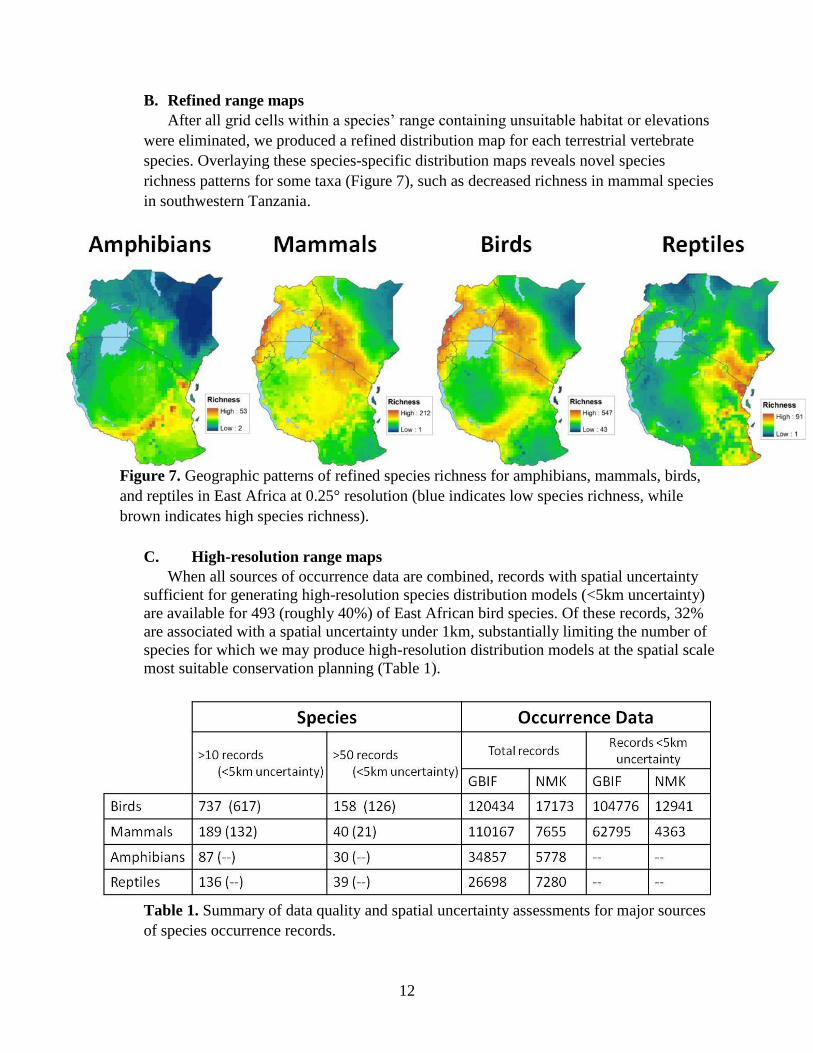
B. Refined range maps

After all grid cells within a species’ range containing unsuitable habitat or elevations

were eliminated, we produced a refined distribution map for each terrestrial vertebrate

species. Overlaying these species-specific distribution maps reveals novel species

richness patterns for some taxa (Figure 7), such as decreased richness in mammal species

in southwestern Tanzania.

Figure 7. Geographic patterns of refined species richness for amphibians, mammals, birds,

and reptiles in East Africa at 0.25° resolution (blue indicates low species richness, while

brown indicates high species richness).

C. High-resolution range maps

When all sources of occurrence data are combined, records with spatial uncertainty

sufficient for generating high-resolution species distribution models (<5km uncertainty)

are available for 493 (roughly 40%) of East African bird species. Of these records, 32%

are associated with a spatial uncertainty under 1km, substantially limiting the number of

species for which we may produce high-resolution distribution models at the spatial scale

most suitable conservation planning (Table 1).

Table 1. Summary of data quality and spatial uncertainty assessments for major sources

of species occurrence records.

13

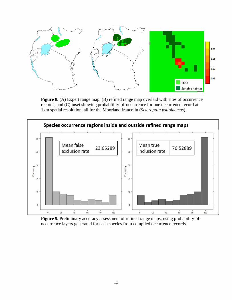
Figure 8. (A) Expert range map, (B) refined range map overlaid with sites of occurrence

records, and (C) inset showing probablility-of-occurrence for one occurrence record at

1km spatial resolution, all for the Moorland francolin (Scleroptila psilolaemus).

Figure 9. Preliminary accuracy assessment of refined range maps, using probability-of-

occurrence layers generated for each species from compiled occurrence records.

Species occurrence regions inside and outside refined range maps

14

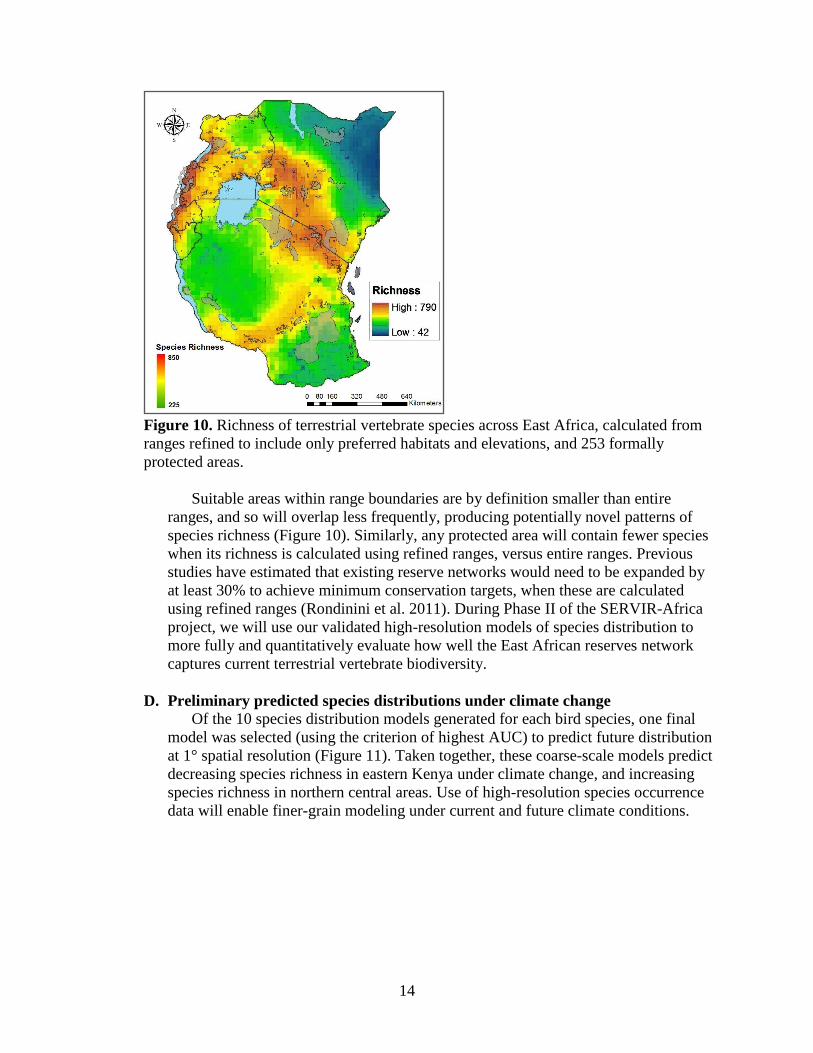
Figure 10. Richness of terrestrial vertebrate species across East Africa, calculated from

ranges refined to include only preferred habitats and elevations, and 253 formally

protected areas.

Suitable areas within range boundaries are by definition smaller than entire

ranges, and so will overlap less frequently, producing potentially novel patterns of

species richness (Figure 10). Similarly, any protected area will contain fewer species

when its richness is calculated using refined ranges, versus entire ranges. Previous

studies have estimated that existing reserve networks would need to be expanded by

at least 30% to achieve minimum conservation targets, when these are calculated

using refined ranges (Rondinini et al. 2011). During Phase II of the SERVIR-Africa

project, we will use our validated high-resolution models of species distribution to

more fully and quantitatively evaluate how well the East African reserves network

captures current terrestrial vertebrate biodiversity.

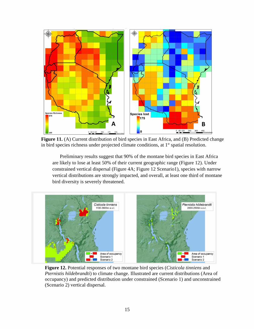
D. Preliminary predicted species distributions under climate change

Of the 10 species distribution models generated for each bird species, one final

model was selected (using the criterion of highest AUC) to predict future distribution

at 1° spatial resolution (Figure 11). Taken together, these coarse-scale models predict

decreasing species richness in eastern Kenya under climate change, and increasing

species richness in northern central areas. Use of high-resolution species occurrence

data will enable finer-grain modeling under current and future climate conditions.

15

Figure 11. (A) Current distribution of bird species in East Africa, and (B) Predicted change

in bird species richness under projected climate conditions, at 1° spatial resolution.

Preliminary results suggest that 90% of the montane bird species in East Africa

are likely to lose at least 50% of their current geographic range (Figure 12). Under

constrained vertical dispersal (Figure 4A; Figure 12 Scenario1), species with narrow

vertical distributions are strongly impacted, and overall, at least one third of montane

bird diversity is severely threatened.

Figure 12. Potential responses of two montane bird species (Cisticola tinniens and

Pternistis hildebrandti) to climate change. Illustrated are current distributions (Area of

occupancy) and predicted distribution under constrained (Scenario 1) and unconstrained

(Scenario 2) vertical dispersal.

A B

16

These results demonstrate the particularly strong climate change impacts that

narrow-ranged, dispersal-limited, and montane species are likely to experience. In

addition, these results show the unique role mountain systems play in determining the

climate change vulnerability.

IV. Phase II proposed research

A. Minimizing uncertainty in high-resolution species distribution models

Over the past decade, important sources of uncertainty in species distribution

models have been identified; these must be specifically addressed in order to generate

reliable models with minimal prediction uncertainty. Several widely used modeling

methods reached 90% of maximum prediction accuracy at 10 occurrence records per

species, setting a convention for minimum sample size for most species distribution

modeling (Stockwell and Peterson 2002). However, larger numbers of occurrence

records are preferred for model precision, refinement, and testing (Elith et al. 2006).

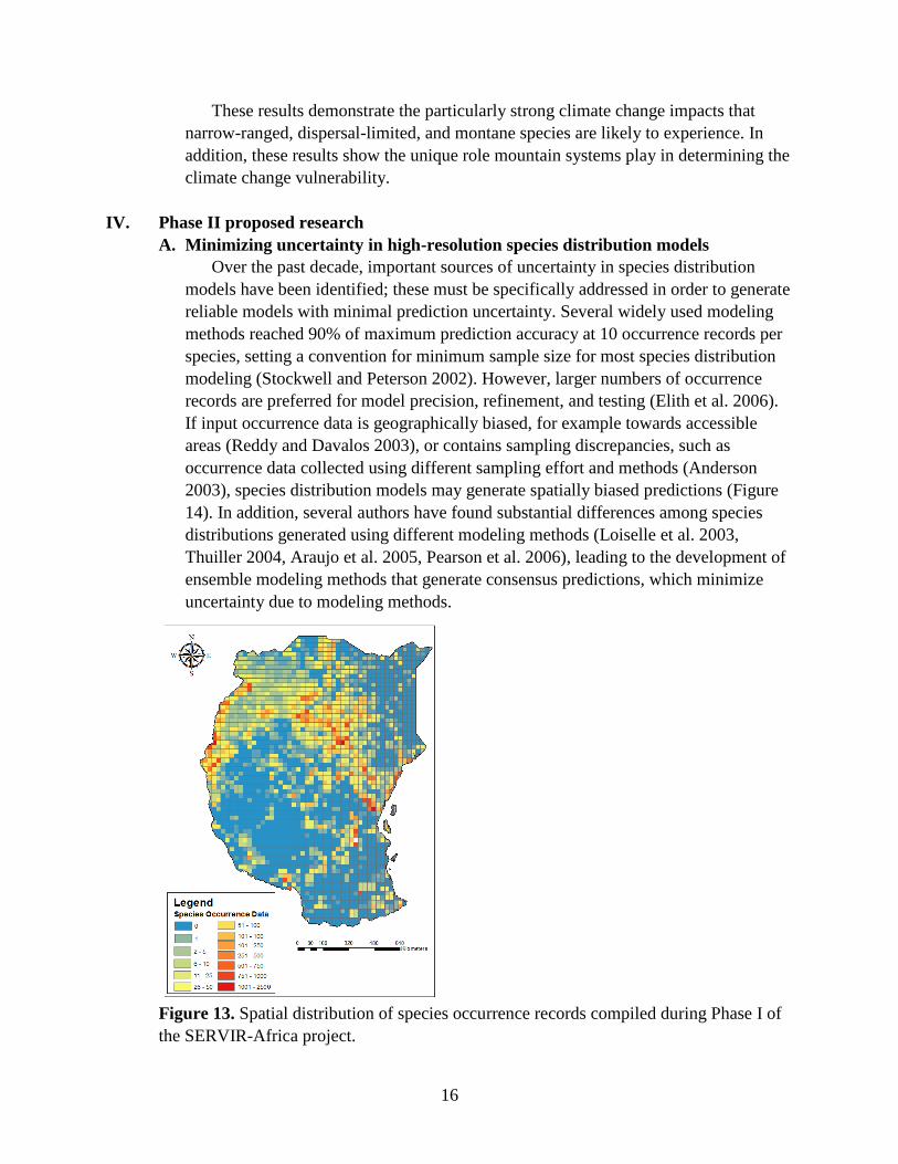
If input occurrence data is geographically biased, for example towards accessible

areas (Reddy and Davalos 2003), or contains sampling discrepancies, such as

occurrence data collected using different sampling effort and methods (Anderson

2003), species distribution models may generate spatially biased predictions (Figure

14). In addition, several authors have found substantial differences among species

distributions generated using different modeling methods (Loiselle et al. 2003,

Thuiller 2004, Araujo et al. 2005, Pearson et al. 2006), leading to the development of

ensemble modeling methods that generate consensus predictions, which minimize

uncertainty due to modeling methods.

Figure 13. Spatial distribution of species occurrence records compiled during Phase I of

the SERVIR-Africa project.

17

However, no investigation has yet explored the effects of the type of occurrence

data on species distribution modeling. Occurrence records may be compiled from

various different types of data, such as reserve checklists, specimens obtained during

a collection expedition (which often describe many different specimens as collected

at the same general location), surveys or other biological sampling effort, or the

scientific literature. These sources of occurrence data clearly differ in observation (or

collection) methods and record-keeping precision, leading, in practice, to large

differences in the nature and amount of spatial uncertainty. For example, species

occurrence data acquired from specimens in natural history collections are often in

the form of a set of coordinates (assigned through retrospective georeferencing) and

an estimate of spatial uncertainty, which combine to produce a circular polygon

representing the spatial region where the species was likely encountered. (As

described above, these polygons range widely in size, though relatively few have a

radius of less than 1 or 5 km.) A second type of species occurrence data might be

acquired from reserve checklists, where the polygonal boundary of the reserve marks

the spatial region where the species was likely encountered.

These two types of spatial distribution data, generated by different types of

species occurrence data, should also differ in the spatial distribution of occurrence

probability. Within the circular polygon, the georeferenced coordinates may or may

not precisely capture the original collection location, but these coordinates, and the

region immediately adjacent to them, nevertheless represent the spatial region most

likely to be the location at which the species was actually encountered. Thus,

probability of occurrence is highest at the center of the circular polygon, and

decreases rapidly toward the edges (during Phase I, we assumed this decrease

followed the form of a negative exponential function). Within the reserve boundaries,

probability of occurrence is spread evenly across the polygon, though likely only over

those areas containing suitable habitat. Thus, any 1km grid cell falling within the

reserve is equally likely to be the location at which the species was actually

encountered.

During Phase II of the SERVIR-Africa project, we will use the species occurrence

data compiled during Phase I, as well as those data generated from additional data

mobilization efforts, to explore the effect of fusing multiple types of species

occurrence data on species distribution modeling. These explorations will contribute

valuable insight into the mechanics of species distribution modeling, and will add to

the growing array of methods available to minimize uncertainty in model results. We

will incorporate existing data quality standards, ensemble modeling methods, and our

own findings regarding the handling of spatial uncertainty for different types of

occurrence data, to produce minimal-uncertainty distribution models for all terrestrial

vertebrate species that occur in East Africa.

18

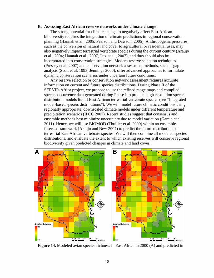
B. Assessing East African reserve networks under climate change

The strong potential for climate change to negatively affect East African

biodiversity requires the integration of climate predictions in regional conservation

planning (Hannah et al., 2005; Pearson and Dawson, 2005). Anthropogenic pressures,

such as the conversion of natural land cover to agricultural or residential uses, may

also negatively impact terrestrial vertebrate species during the current century (Araújo

et al., 2004; Hannah et al., 2007, Jetz et al., 2007), and thus should also be

incorporated into conservation strategies. Modern reserve selection techniques

(Pressey et al. 2007) and conservation network assessment methods, such as gap

analysis (Scott et al. 1993, Jennings 2000), offer advanced approaches to formulate

dynamic conservation scenarios under uncertain future conditions.

Any reserve selection or conservation network assessment requires accurate

information on current and future species distributions. During Phase II of the

SERVIR-Africa project, we propose to use the refined range maps and compiled

species occurrence data generated during Phase I to produce high-resolution species

distribution models for all East African terrestrial vertebrate species (see “Integrated

model-based species distributions”). We will model future climatic conditions using

regionally appropriate, downscaled climate models under different temperature and

precipitation scenarios (IPCC 2007). Recent studies suggest that consensus and

ensemble methods best minimize uncertainty due to model variation (Garcia et al.

2011). Hence, we will use BIOMOD (Thuiller et al. 2009) within an ensemble

forecast framework (Araujo and New 2007) to predict the future distributions of

terrestrial East African vertebrate species. We will then combine all modeled species

distributions, and evaluate the extent to which existing reserves will conserve regional

biodiversity given predicted changes in climate and land cover.

Figure 14. Modeled avian species richness in East Africa in 2000 (A) and predicted in

19

2100 (B), at 1° spatial resolution. (For methods, see section “Preliminary predicted

species distributions under climate change.”)

Overlaying current avian richness with the East African reserve network (Figure

14A) shows generally poor overlap between protected areas and the occupied areas of

species’ ranges. These results, while strictly qualitative and limited to coarse spatial

scales, are congruent with other findings that existing African reserves, often created

for an individual species or on an ad hoc basis, do not include sufficient proportions

of many species’ ranges, and still less of a species’ occupied or suitable area (de

Klerk et al. 2004, Fjeldsa et al. 2004, Rondinini 2005, Beresford 2010). These results

are not particularly surprising, given that species’ suitable areas, by definition, are

smaller and overlap less than species’ geographic ranges, but do not paint a positive

picture of the current level of regional biodiversity conservation. During Phase II of

the SERVIR-Africa project, we will more fully evaluate how well the East African

reserves network captures the current distributions of all terrestrial vertebrate species,

at 1-5km spatial resolution.

Preliminary analyses of bird species distributions under climate change suggest

that future species richness patterns will diverge from current-day patterns (Figure

14B). That such alterations to species distributions are apparent at even coarse spatial

scales implies a startlingly high rate of species turnover. Using our high-resolution

models of current species distributions as inputs to the BIOMOD ensemble modeling

framework, we will produce much more detailed predictions of future distributions.

These fine-grain predictions will, in turn, enable a full and quantitative evaluation of

changes to regional species distribution patterns, as well as the capacity of the East

African reserve network to conserve terrestrial vertebrate biodiversity under climate

change.

This whole-network approach has already proven valuable in multiple

conservation contexts. In Europe, climate change is predicted to decrease the climatic

suitability of protected areas for approximately 58% of plant and terrestrial vertebrate

species by 2080 (Araujo et al. 2011). The Brazilian reserve system was found to fail

even more dramatically under climate change, losing all coverage of suitable climate

for 38 bird species by 2060 (Marini et al. 2009). Finally, Hole et al. (2009) predict

that future alterations to climatic conditions in Important Bird Areas (IBAs) in Africa

will decrease the representation of priority bird species by 51-56% over the next

century.

Following our production of fine-grain predictions of species distributions under

climate change, we will evaluate how well existing East African protected areas

capture future species diversity and richness patterns. Based on an array of potential

conservation goals, including multitaxon minimum sets, maximizing

complementarity, and proportional representation (Kremen et al. 2008), we will

recommend priority locations for formal protection and conservation action. We will

also emphasize conservation targets specific to endemic species, as well as those

terrestrial vertebrate species important for tourism and other regional industries. Our

Phase II products will provide comprehensive, spatially detailed information tailored

to regional conservation priorities, supporting long-term conservation planning and

policy development.

20

References

Alroy, J. 2002 How many named species are valid? Proceedings of the National Academy of

Sciences 99: 3706–3711.

Anderson, TM, Metzger, KL, and SJ Naughton. 2007. Multi-scale analysis of plant species

richness in Serengeti grasslands. Journal of Biogeography 34(2): 313–323.

Araújo, MB, Alagador, D, Cabeza, M, Nogues-Bravo, N, and W Thuiller. 2011. Climate change

threatens European conservation areas. Ecology letters 14: 484–492.

Araujo, MB, and M New. 2007. Ensemble forecasting of species distributions. Trends in

Ecology and Evolution 22: 42–47.

Araújo, MB, Pearson, RG, Thuiller, W, and M Erhard. 2005. Validation of species–climate

impact models under climate change. Global Change Biology 11(9): 1504-1513.

Araújo, MB, Thuiller, W, and NG Yoccoz. 2009. Reopening the climate envelope reveals

macroscale associations with climate in European birds. PNAS 106(16): E45-E46.

Araujo, MB. 2004. Matching species with reserves - uncertainties from using data at different

resolutions. Biological Conservation 118: 533–538.

Augustine, D. 2003. Spatial heterogeneity in the herbaceous layer of a semi-arid savanna

ecosystem. Plant Ecology 167: 319-332.

Beaman, R, Wieczorek, J, and S Blum. 2004. Determining Space from Place for Natural History

Collections in a Distributed Digital Library Environment. D-Lib Magazine 10(5)

doi:10.1045/may2004-beaman.

Belmaker, J, and WJ Jetz. Cross-scale variation in species richness–environment associations.

Global Ecology and Biogeography. Published online November 16, 2010.

Bennun, L., and P. Njoroge. 1999. Important Bird Areas in Kenya. NatureKenya, East Africa

Natural History Society, PO Box 44486, Nairobi, Kenya.

Beresford, AE, Buchanan, GM, Donald, PF, Butchart, SHM, L. Fishpool, DC, and C Rondinini.

2010. Poor overlap between the distribution of Protected Areas and globally threatened birds

in Africa. Animal Conservation (2010):1-9.

Boone, RB, and WB Krohn. 1999. Modeling the occurrence of bird species: are the errors

predictable? Ecological Applications 9:835–848

Boyle, B.L. 2006. TaxonScrubber, Version 2.0. The SALVIAS Project,

http://www.salvias.net/pages/taxonscrubber.html.

Brooks, T, Balmford, A, Burgess, N, Fjeldsa, J, Hansen, LA, Moore, J, Rahbek, C, and P

Williams. 2001. Towards a blueprint for conservation in Africa. BioScience 51: 613–624.

Burgess, ND, Balmford, A, Cordeiro, NJ, Fjeldsa, J, Kuper, W, Rahbek, C, Sanderson, EW,

Scharlemann, JPW, Sommer, JH, and PH Williams. 2007b. Correlations among species

distributions, human density and human infrastructure across the high biodiversity tropical

mountains of Africa. Biological Conservation 134(2): 164-177.

Burgess, ND, Butynski, TM, Cordeiro, NJ, Doggart, NN, Fjeldsa, J, Howell, KM, Kilahama,

FB, Loader, FB, Lovett, JC, Mbilinyi, B, Menegon, M, Moyer, DC, Nashanda, E, A. Perkin,

Rovero, F, Stanley, WT, and SN Stuart. 2007a. The biological importance of the Eastern Arc

Mountains of Tanzania and Kenya. Biological Conservation 134: 209–231.

Burgess, ND, Clarke, GP, Madgwick, J, Robertson, SA, and A Dickinson. 2000. Status and

vegetation; distribution and status. Pp. 71–81 in ND Burgess and GP Clarke (eds.), Coastal

Forests of Eastern Africa. IUCN Forest Conservation Programme, Gland, Switzerland and

Cambridge, UK.

Burgess, N, de Klerk, H, Fjeldså, J, Crowe, T, and C Rahbek. 2000. A preliminary assessment

of congruence between biodiversity patterns in Afrotropical forest birds and forest mammals.

21

Ostrich 71: 286–290.

Burgess, ND, Fjeldså, J, and C Rahbek. 1998a. Mapping the distributions of Afrotropical

vertebrate groups. Species 30: 16–17.

Burgess, ND, Fjeldså, J, and R Botterweg. 1998b. Faunal Importance of the Eastern Arc

Mountains of Kenya and Tanzania. Journal of East African Natural History 87(1):37-58.

Chapin, JP. 1923. Ecological Aspects of Bird Distribution in Tropical Africa. The American

Naturalist 57(649): 106-125 .

Chapman, A.D. 2005. Principles of Data Quality. Report for the Global Biodiversity Information

Facility, Copenhagen.

Chapman, AD, and J Wieczorek (eds). 2006. Guide to BestPractices for Georeferencing. Global

Biodiversity Information Facility: Copenhagen, Denmark.

Coe, MJ, Cumming, DH, and J Phillipson. 1976, Biomass and production of large African

herbivores in relation to rainfall and primary production. Oecologia 22: 341-354.

Collen, B, Ram, M, Zamin, T, and L McRae. 2008. The tropical biodiversity data gap:

addressing disparity in global monitoring. Tropical Conservation Science 1(2): 75-88.

Crowe, TM, and AA Crowe. 1982. Patterns in distribution, diversity, and endemism in

Afrotropical birds. Journal of Zoology 198: 417–442.

Currie, DJ, Mittelbach, GG, Cornell, HV, Field, R, Guégan, JF, Hawkins, BA, Kaufman, DM,

Kerr, JT, Oberdorff, T, O’Brien, E, and JRG Turner. 2004. Predictions and tests of climate-

based hypotheses of broad-scale variation in taxonomic richness. Ecology Letters 7: 1121–

1134.

De Klerk, HM, Crowe, TM, Fjeldsa, J, and ND Burgess. 2002a. Biogeographical patterns of

endemic terrestrial Afrotropical birds. Diversity and Distributions 8(3): 147–162.

De Klerk, HM, Crowe, TM, Fjeldsa, J, and ND Burgess. 2002b. Patterns of species richness and

narrow endemism of terrestrial bird species in the Afrotropical region. Journal of Zoology

256: 327-342.

Dillon, S, and J Fjeldså. 2005. The implications of different species concepts for describing

biodiversity patterns and assessing conservation needs for African birds. Ecography 28: 682–

692.

Elith, J. et al. 2006 Novel methods improve prediction of species’ distributions from occurrence

data. Ecography 29, 129–151.

Emmerson, M., Bezemer, M, Hunter, MD, and TH Jones. 2005. Global change alters the stability

of food webs. Global Change Biology 11(3): 490-501.

Fahr, J, and EKV Kalko. 2010. Biome transitions as centres of diversity: habitat heterogeneity

and diversity patterns of West African bat assemblages across spatial scales. Published

online August 13, 2010.

Ferrier, S. 2002. Mapping spatial pattern in biodiversity for regional conservation planning:

where to from here? Systematic Biology. 51: 331-363.

Fjeldsa, J. 2007. How broad-scale studies of patterns and processes can serve to guide

conservation planning in Africa. Conservation Biology 21(3): 659-667.

Gaston, KJ and RA Fuller. 2009. The sizes of species’ geographic ranges. Journal of Applied

Ecology, 46: 1–9.

Graham, CH, Ferrier, S, Huettman, F, Moritz, C, and AT Peterson. 2004. New developments in

museum-based informatics and applications in biodiversity analysis. TRENDS in Ecology

and Evolution 19(9): 497-503.

Guisan, A. and W. Thuiller 2005. Predicting species distribution: offering more than simple

habitat models. Ecology Letters 8(9): 993-1009.

22

Guisan, A. & Zimmermann, N. E. 2000 Predictive habitat distribution models in ecology. Ecol.

Model. 135: 147–186.

Guralnick, R, and A Hill. 2009. Biodiversity informatics: automated approaches for documenting

global biodiversity patterns and processes. Bioinformatics 25(4): 421-428.

Guralnick RP, Wieczorek J, Beaman R, and RJ Hijmans. 2006. BioGeomancer: Automated

Georeferencing to Map the World's Biodiversity Data. PLoS Biology 4(11): e381.

Hannah, L., Midgley, G.F., Andelman, S., Arau´jo, M.B., Hughes, G., Martinez-Meyer, E. et al.

2007. Protected area needs in a changing climate. Frontiers in Ecology and the Environment

5: 131–138.

Hawkins, BA, Field, R, Cornell, HV, Currie,DJ, Guégan, JF, Kaufman, DM, Kerr, JT,

Mittelbach, GG, Oberdorff, T, and EM O’Brien. 2003. Energy, water, and broad-scale

geographic patterns of species richness. Ecology, 84: 3105–3117.

Hole, DG, Willis, SG, Pain, DJ, Fishpool, LD, Butchart, SHM, Collingham, YC, et al. 2009.

Projected impacts of climate change on a continent-wide protected area network. Ecology

Letters 12: 420–431.

Homewood, K, Lambin, E, Coast, E, Kariuki, A, Kivelia, J, Said, M, Serneels, S, and M

Thompson. 2001. Long-term changes in Serengeti-Mara wildebeest and land cover:

pastoralism, population, or policies? Proceedings of the National Academy of Sciences 98:

12544–12549.

Hortal, J. 2008. Uncertainty and the measurement of terrestrial biodiversity gradients. Journal of

Biogeography 35: 1335–1336.

Hurlbert, AH, and EP White. 2005. Disparity between range map- and survey-based analyses of

species richness: patterns, processes and implications. Ecology Letters 8(3): 319–327.

IUCN and UNEP. 2010. The World Database on Protected Areas (WDPA). UNEP-WCMC:

Cambridge, UK.

Jefferson TA, Jenkins RK, Johnston CH, Keith M, Kingdon J, Knox DH, Kovacs KM,

Langhammer P, Leus K, Lewison R, Lichtenstein G, Lowry LF, Macavoy Z, Mace GM,

Mallon DP, Masi M, McKnight MW, Medellín RA, Medici P, Mills G, Moehlman PD,

Molur S, Mora A, Nowell K, Oates JF, Olech W, Oliver WR, Oprea M, Patterson BD, Perrin

WF, Polidoro BA, Pollock C, Powel A, Protas Y, Racey P, Ragle J, Ramani P, Rathbun G,

Reeves RR, Reilly SB, Reynolds JE 3rd, Rondinini C, Rosell-Ambal RG, Rulli M, Rylands

AB, Savini S, Schank CJ, Sechrest W, Self-Sullivan C, Shoemaker A, Sillero-Zubiri C, De

Silva N, Smith DE, Srinivasulu C, Stephenson PJ, van Strien N, Talukdar BK, Taylor BL,

Timmins R, Tirira DG, Tognelli MF, Tsytsulina K, Veiga LM, Vié JC, Williamson EA,

Wyatt SA, Xie Y, and BE Young. 2008. The status of the world's land and marine mammals:

diversity, threat, and knowledge. Science 322(5899): 225-230.

Jetz, W, and C Rahbek. 2001. Geometric constraints explain much of the species richness pattern

in African birds. Proceedings of the National Academy of Sciences 98(10): 5661-5666.

Jetz, W, and C Rahbek. 2002. Geographic range size and determinants of avian species richness.

Science 297: 1548–1551.

Jetz W, Wilcove DS, and AP Dobson. 2007 Projected Impacts of Climate and Land-Use Change

on the Global Diversity of Birds. PLoS Biol 5(6):e157.

Jetz, W., Sekercioglu C, and JEM Watson. 2008. Ecological correlates and conservation

implications of overestimating species’ geographic ranges. Conservation Biology 22: 110-

119.

Kremen, C. et al. 2008. Aligning conservation priorities across taxa in Madagascar with high-

resolution planning tools. Science 320: 222–226.

23

Kuper, W, Sommer, JH, Lovett, JC, and W Barthlott. 2006. Deficiency in African plant

distribution data – missing pieces of the puzzle. Botanical Journal of the Linnean Society

150(3): , 355–368.

Langhammer, P.F., M.I. Bakarr, L.A. Bennun, T.M. Brooks, R.P. Clay, R.P., W. Darwall, N. De

Silva, G.J. Edgar, G. Eken, L.D.C. Fishpool, G.A.B. de Fonseca, M.N. Foster, D.H. Knox, P.

Matiku, E.A. Radford, A.S.L. Rodigues, P. Salaman, W. Sechrest, & A.W. Tordoff. 2007.

Identification and Gap Analysis of Key Biodiversity Areas: Targets for Comprehensive

Protected Area Systems. IUCN, Gland, Switzerland.

Larsen, FW, and C Rahbek. 2005. The influence of spatial grain size on the suitability of the

higher-taxon approach in continental priority-setting. Animal Conservation 8: 389–396.

Le Houerou, HN, and CH Hoste. 1977. Rangeland production and annual rainfall relations in the

Mediterranean basin and in the African Sahelo-Soudanian zone. Journal of Range

Management 30: 181-189.

Loiselle, BA, Howell, CA, Graham, CH, Goerck, JM, Brooks, TM, Smith, KG, and PH

Williams. 2003. Avoiding pitfalls of using species distribution models in conservation

planning. Conservation Biology 17: 1591–1600.

McLaughlin, JF, Hellmann, JJ, Boggs, CL, and PR Ehrlich. 2002. Climate change hastens

population extinctions. Proceedings of the National Academy of Sciences of the United

States of America 99: 6070–6074.

McNaughton, SJ. 1985. Ecology of a Grazing Ecosystem: The Serengeti. Ecological

Monographs 55(3): 259-294.

McPherson, JM and W Jetz. 2000. Type and spatial structure of distribution data and the

perceived determinants of geographical gradients in ecology: the species richness of African

birds. Global Ecology and Biogeography 16: 657–667.

McPherson, JM, Jetz, W, and DJ Rogers. 2006. Using coarse-grained occurrence data to predict

species distributions at finer spatial resolutions--possibilities limitations. Ecological

Modeling 192(4): 499-522.

Marini MA et al., 2009. Predicted climate-driven bird distribution changes and forecasted

conservation conflicts in a neotropical savanna. Conservation Biology 23:1558-1567.

Murphey, PC, Guralnick, RP, Glaubitz, R, Neufeld, D, and JA Ryan. 2004. Georeferencing of

museum collections: A review of problems and automated tools, and the methodology

developed by the Mountain and Plains Spatio-Temporal Database-Informatics Initiative

(Mapstedi). PhyloInformatics 3: 1-29 – 2004

Myers, N, Mittermeier, RA, Mittermeier, GA, da Fonseca, GAB, and J Kent. 2000. Biodiversity

hotspots for conservation priorities. Nature 403: 853–858.

Parmesan, C, and G Yohe. A globally coherent fingerprint of climate change impacts across

natural systems. 2003. Nature 421: 37–42.

Pearson, R. G. and TP Dawson. 2003. Predicting the impacts of climate change on the

distribution of species: are bioclimate envelope models useful? Global Ecology and

Biogeography 12(5): 361-371.

Pennycuick, L. 1975. Movements of the migratory wildebeest population in the Serengeti Area

between 1960 and 1973. Journal of East African Wildlife 13: 65-87.

Plumptre, AJ, Davenport, TRB, Behangana, M, Kityo, R, Eilu, G, Ssegawa, P, Ewango, C,

Meirte, D, Kahindo, C, Herremans, M, Peterhans, JK, Pilgrim, JD, Wilson, M, Languy, M,

and D Moyer. 2007a. The biodiversity of the Albertine Rift. Biological Conservation 134(2):

178-194.

Plumptre, AJ, Kujirakwinja, D, Treves, D, Owiunji, I, and H. Rainer. 2007b. Transboundary

24

Conservation in the Greater Virunga Landscape: its importance for Landscape Species.

Biological Conservation 134: 279–287.

Pounds AJ, Bustamante MR, Coloma LA, Consuegra JA, and Fogden MPL. 2006. Widespread

amphibian extinctions from epidemic disease driven by global warming. Nature 439: 161–

167.

Pressey, RL, Cabeza, M, Watts, ME, Cowling, RM, and KA Wilson. 2007. Conservation

planning in a changing world, Trends in Ecology Evolution 22(11): 583-592.

Price, B., C.A. McAlpine, A.S. Kutt, S.R. Phinn, D.V. Pullar, and J.A. Ludwig. 2009.

Continuum or discrete patch landscape models for savanna birds: Towards a pluralistic

approach. Ecography 32:745-756.

Prins, E, and P Clarke. 2006. Discovery and enumeration of the Swahilian Coastal Forests in the

Lindi region, Tanzania, using Landsat TM data analysis. Biodiversity Conservation 16(5):

1551–1565.

Rahbek, C, and GR Graves. 2000. Detection of macro-ecological patterns in South American

hummingbirds is affected by spatial scale. Proceedings of the Royal Society B: Biological

Sciences. 267: 2259–2265.

Rahbek, C, and GR Graves. 2001. Multiscale assessment of patterns of avian species richness.

Proceedings of the National Academy of Sciences 98(8): 4534-4539.

Reddy, S. and LM Davalos. 2003. Geographical sampling bias and its implications for

conservation priorities in Africa. Journal of Biogeography 30: 1719–1727.

Ricklefs, RE. 2004. A comprehensive framework for global patterns in biodiversity. Ecology

Letters 7: 1–15.

Rodrigues, ASL, et al. 2011. Complete, accurate, mammalian phylogenies aid conservation

planning, but not much. Phil. Trans. R. Soc. B 366, 2652–2660.

Romdal, TS, and C Rahbek. 2009. Elevation zonation of Afrotropical forest bird communities

along a homogenous forest gradient. Journal of Biogeography 36: 327-336.

Root, TL, Price, JT, Hall, KR, Schneider, SH, and C Rosenzweig. 2003. Fingerprints of global

warming on wild animals and plants. Nature 421: 57–60.

Rondinini, C, Wilson, KA, Biotani, L, Grantham, H, and HP Possingham. 2004. Tradeoffs of

different types of species occurrence data for use in systematic conservation planning.

Ecology Letters 9(10): 1136–1145.

Rondinini, C, Stuart, S, and L Boitani. 2005 Habitat suitability models and the shortfall in

conservation planning for African vertebrates. Conservation Biology 19, 1488–1497.

Rouget, M. 2003. Measuring conservation value at fine and broad scales: implications for a

diverse and fragmented region, the Agulhas Plain. Biological Conservation 112:217-232.

Scott, J.M., Heglund, P.J., Morrison, M.L., Haufler, J.B., Raphael, M.G., Wall, W.A. et al. (eds).

2002 Predicting Species Occurrences: Issues of Accuracy and Scale. Island Press,

Washington, DC.

Shmida, A, and MV Wilson. 1985. Biological determinants of species diversity. Journal of

Biogeography 12: 1–20.

Sibley, CG, and BL Monroe Jr. 1996. Birds of the World. Yale University Press: New Haven,

CT, United States.

Sinclair, ARE, Mduma, SAR. Hopcraft, JGC, Fryxell, JM, Hilborn, R, and S Thirgood. 2007.

Long-term ecosystem dynamics in the Serengeti: lessons for conservation. Conservation

Biology 21:580–590.

25

Spawls, S. 2004. A field guide to the reptiles of East Africa: Kenya, Tanzania, Uganda, Rwanda

and Burundi. Academic, San Diego, CA, USA.

Soberon, J, and AT Peterson. 2004. Biodiversity informatics: managing and applying primary

biodiversity data. Philosophical Transactions of the Royal Society B: Biological Sciences

359: 689–698.

Stockwell, DRB, and AT Peterson. 2002. Effects of sample size on accuracy of species

distribution models. Ecological Modelling 148: 1-13.

Tabor, K, Burgess, ND, Mbilinyi, BP, Kashaigili, JJ, and MK Steininger. 2010. Forest and

Woodland Cover and Change in Coastal Tanzania and Kenya, 1990 to 2000.. Journal of East

African Natural History 99(1): 19-45.

Thomas, CD, and JJ Lennon. 1999. Birds extend their ranges northwards. Nature 399: 213.

Thuiller, W, Lavorel, S, Araujo, MB, Sykes, MT, and IC Prentice. 2005. Climate change threats

to plant diversity in Europe. Proceedings of the National Academy of Sciences U.S.A., 102:

8245–8250.

Thuiller, W, Lafourcade, B, Engler, R, and MB Araujo. 2009. BIOMOD – A platform for

ensemble forecasting of species distributions. Ecography, 32: 369–373.

Tilman, D, Knops, J, Wedin, D, Reich, P, and M Ritchie. 1997. The Influence of Functional

Diversity and Composition on Ecosystem Processes. Science 277(5330): 1300-1302.

Walther, GR, Post, E, Convey, P, Menzel, A, and C Parmesan. 2002. Ecological responses to

recent climate change. Nature 416: 389–395.

Western, D. 1975. Water availability and its influence on the structure and dynamics of a

savannah large mammal community. Journal of East African Wildlife 13: 265–286.

White, EP, and AH Hurlbert. 2010. The combined influence of the local environment and

regional enrichment on bird species richness. The American Naturalist 175(2): E35-43.

Whittaker, RJ, Willis, KJ, and R Field. 2001. Scale and species richness: towards a general,

hierarchical theory of species diversity. Journal of Biogeography 28: 453–470.

Wieczorek, JR. 2001. MaNIS/VertNet/ORBIS Georeferencing Guidelines,

(http://elib.cs.berkeley.edu/manis/GeorefGuide.html)

Wieczorek, J, Guo, Q, and RJ Hijmans. 2004. The point-radius method for georeferencing

locality descriptions and calculating associated uncertainty. International Journal of

Geographical Information Science, 18: 745–767.

Williams, PH, de Klerk, HM, and TM Crowe. 1999. Interpreting biogeographical boundaries

among Afrotropical birds: spatial patterns in richness gradients and species replacement.

Journal of Biogeography, 26, 459–474.

Williams, PH, Burgess, ND, and C Rahbek. 2000. Flagship species, ecological complementarity

and conserving the diversity of mammals and birds in sub-Saharan Africa. Animal

Conservation, 3: 249–260.

Williams, PH, Margules, CR, and DW Hilbert. 2002. Data requirements and data sources for

biodiversity priority area selection. Journal of Bioscience 27: 327–338.

World Tourism Organisation (WTO). 2006. Tourism market trends.

http://www.unwto.org/facts/eng/pdf/indicators/new/ITR05_africa_US$.pdf.

Yesson C, Brewer PW, Sutton T, Caithness N, and JS Pahwa. 2007. How Global Is the Global

Biodiversity Information Facility? PLoS ONE 2(11): e1124.