Embed Size (px)
Citation preview
SFU, CMPT 741, Fall 2009, Martin Ester 1
Cluster and Outlier AnalysisContents of this Chapter
Introduction (sections 7.1 – 7.3)
Partitioning Methods (section 7.4)
Hierarchical Methods (section 7.5)
Density-Based Methods (section 7.6)
Database Techniques for Scalable Clustering
Clustering High-Dimensional Data (section 7.9)
Constraint-Based Clustering (section 7.10)
Outlier Detection (section 7.11)
Reference: [Han and Kamber 2006, Chapter 7]
SFU, CMPT 741, Fall 2009, Martin Ester 2
IntroductionGoal of Cluster Analysis
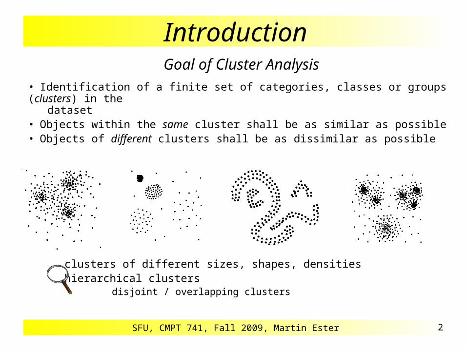
• Identification of a finite set of categories, classes or groups (clusters) in the dataset• Objects within the same cluster shall be as similar as possible• Objects of different clusters shall be as dissimilar as possible
clusters of different sizes, shapes, densitieshierarchical clusters
disjoint / overlapping clusters

SFU, CMPT 741, Fall 2009, Martin Ester 3
IntroductionGoal of Outlier Analysis
• Identification of objects (outliers) in the dataset which aresignificantly different from the rest of the dataset (global outliers)or significantly different from their neighbors in the dataset (local outliers)
outliers do not belong to any of the clusters
..
global outliers
local outlier
SFU, CMPT 741, Fall 2009, Martin Ester 4
IntroductionClustering as Optimization Problem
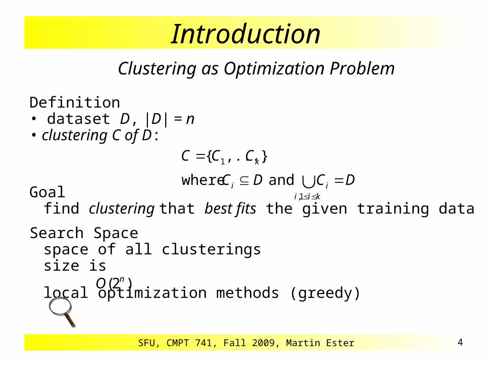
Definition• dataset D, |D| = n• clustering C of D:
Goalfind clustering that best fits the given training data
Search Spacespace of all clusteringssize is
local optimization methods (greedy)
DCDC
CCC
kiiii
k
1,
1
andwhere
},...,{
)2( nO
SFU, CMPT 741, Fall 2009, Martin Ester 5
IntroductionClustering as Optimization Problem
Steps
1. Choice of model category partitioning, hierarchical, density-based
2. Definition of score function typically, based on distance function
3. Choice of model structure feature selection / number of clusters
4. Search for model parameters clusters / cluster representatives
SFU, CMPT 741, Fall 2009, Martin Ester 6
Distance FunctionsBasics
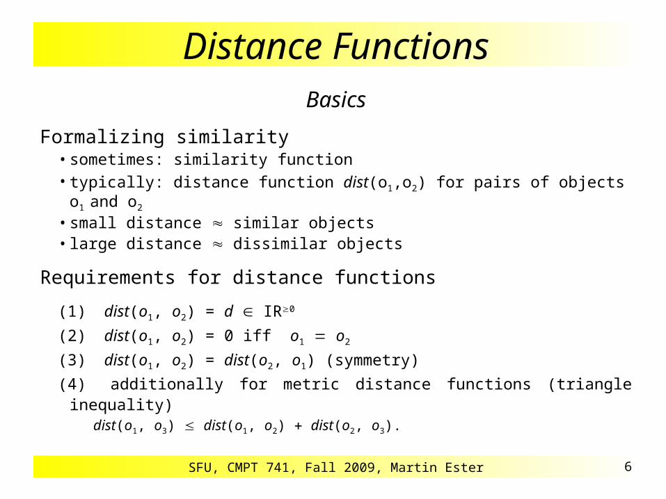
Formalizing similarity• sometimes: similarity function• typically: distance function dist(o1,o2) for pairs of objects o1 and o2
• small distance similar objects• large distance dissimilar objects
Requirements for distance functions
(1) dist(o1, o2) = d IR0
(2) dist(o1, o2) = 0 iff o1 o2
(3) dist(o1, o2) = dist(o2, o1) (symmetry)
(4) additionally for metric distance functions (triangle inequality)dist(o1, o3) dist(o1, o2) dist(o2, o3).
SFU, CMPT 741, Fall 2009, Martin Ester 7
Distance Functions
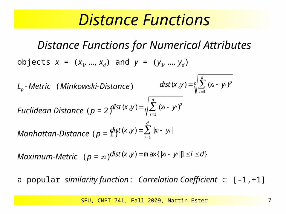
Distance Functions for Numerical Attributes
objects x = (x1, ..., xd) and y = (y1, ..., yd)
Lp-Metric (Minkowski-Distance)
Euclidean Distance (p = 2)
Manhattan-Distance (p = 1)
Maximum-Metric (p = )
a popular similarity function: Correlation Coefficient [-1,+1]
dist x y x yi ip
i
d
p( , ) ( )
1
dist x y x yi i
i
d
( , ) ( ) 2
1
dist x y x yi i
i
d
( , ) | |
1
dist x y x y i di i( , ) max{| || } 1
SFU, CMPT 741, Fall 2009, Martin Ester 8
Distance Functions
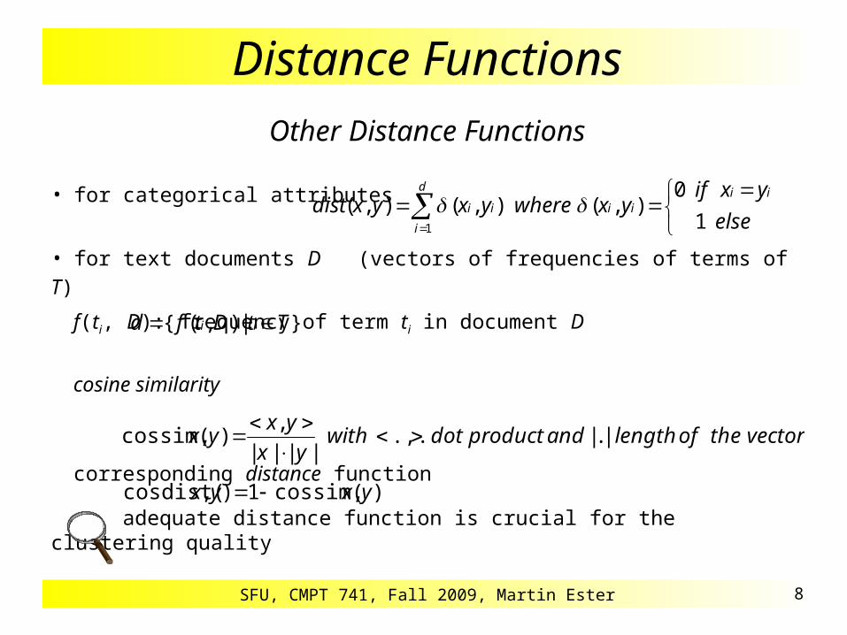
Other Distance Functions
• for categorical attributes
• for text documents D (vectors of frequencies of terms of T)
f(ti, D): frequency of term ti in document D
cosine similarity
corresponding distance function
adequate distance function is crucial for the clustering quality
d
i
iiiiii
else
yxifyxwhereyxyxdist
1 1
0),(),(),(
}|),({ TtDtfd ii
vectortheoflengthandproductdotwithyx
yxyx |.|.,.
||||
,),cossim(
),cossim(1),cosdist( yxyx

SFU, CMPT 741, Fall 2009, Martin Ester 9
Typical Clustering Applications
Overview
• Market segmentation
clustering the set of customer transactions
• Determining user groups on the WWW
clustering web-logs
• Structuring large sets of text documents
hierarchical clustering of the text documents
• Generating thematic maps from satellite images
clustering sets of raster images of the same area (feature vectors)

SFU, CMPT 741, Fall 2009, Martin Ester 10
Typical Clustering Applications
Determining User Groups on the WWW
Entries of a Web-Log
Sessions
Session::= <IP-Adress, User-Id, [URL1, . . ., URLk]>
which entries form a session?
Distance Function for Sessions
romblon.informatik.uni-muenchen.de lopa - [04/Mar/1997:01:44:50 +0100] "GET /~lopa/ HTTP/1.0" 200 1364romblon.informatik.uni-muenchen.de lopa - [04/Mar/1997:01:45:11 +0100] "GET /~lopa/x/ HTTP/1.0" 200 712fixer.sega.co.jp unknown - [04/Mar/1997:01:58:49 +0100] "GET /dbs/porada.html HTTP/1.0" 200 1229scooter.pa-x.dec.com unknown - [04/Mar/1997:02:08:23 +0100] "GET /dbs/kriegel_e.html HTTP/1.0" 200 1241
tCoefficienJaccardyx
yxyxyxd
||
||||),(
SFU, CMPT 741, Fall 2009, Martin Ester 11
Typical Clustering Applications
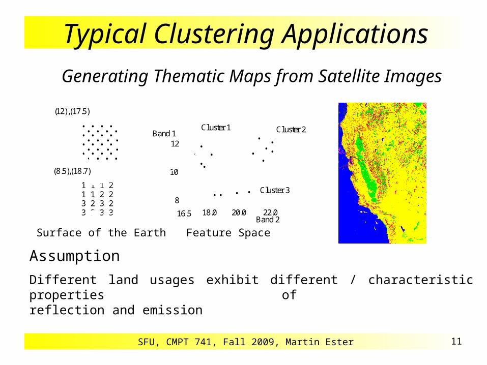
Generating Thematic Maps from Satellite Images
Assumption
Different land usages exhibit different / characteristic properties of reflection and emission
• • • •• • • •• • • •• • • •
• • • •• • • •• • • •• • • •
Erdoberfläche Feature-Raum
Band 1
Band 216.5 22.020.018.0
8
12
10
•
(12),(17.5)
(8.5),(18.7)
•• •
•
••• •
••
••••1 1 1 21 1 2 23 2 3 23 3 3 3
Cluster 1 Cluster 2
Cluster 3
Surface of the Earth Feature Space

SFU, CMPT 741, Fall 2009, Martin Ester 12
Types of Clustering MethodsPartitioning Methods
• Parameters: number k of clusters, distance function• determines a „flat“ clustering into k clusters (with minimal costs)
Hierarchical Methods• Parameters: distance function for objects and for clusters• determines a hierarchy of clusterings, merges always the most similar
clusters
Density-Based Methods• Parameters: minimum density within a cluster, distance function• extends cluster by neighboring objects as long as the density is large enough
Other Clustering Methods• Fuzzy Clustering• Graph-based Methods• Neural Networks

SFU, CMPT 741, Fall 2009, Martin Ester 13
Partitioning MethodsBasics
Goal
a (disjoint) partitioning into k clusters with minimal costs
Local optimization method
• choose k initial cluster representatives
• optimize these representatives iteratively
• assign each object to its most similar cluster representative
Types of cluster representatives
• Mean of a cluster (construction of central points)
• Median of a cluster (selection of representative points)
• Probability density function of a cluster (expectation maximization)

SFU, CMPT 741, Fall 2009, Martin Ester 14
Construction of Central Points
1
1
5
5
x Centroide
x
xx
1
1
5
5
x Centroidex
x
x
1
1
5
5
1
1
5
5
Example
Cluster Cluster Representatives
bad clustering
optimal clustering

SFU, CMPT 741, Fall 2009, Martin Ester 15
Construction of Central Points
Basics [Forgy 1965]
• objects are points p=(xp1, ..., xp
d) in an Euclidean vector space
• Euclidean distance
• Centroid C: mean vector of all objects in cluster C
• Measure for the costs (compactness) of a clusters C
• Measure for the costs (compactness) of a clustering
TD C dist p C
p C
2 2( ) ( , )
TD TD Ci
i
k2 2
1
( )

SFU, CMPT 741, Fall 2009, Martin Ester 16
Construction of Central Points
Algorithm
ClusteringByVarianceMinimization(dataset D, integer k) create an „initial“ partitioning of dataset D into k clusters;
calculate the set C’={C1, ..., Ck} of the centroids of the k clusters;
C = {};repeat until C C’
C = C’;form k clusters by assigning each object to the closest centroid from C;
re-calculate the set C’={C’1, ..., C’k} of the centroids for the newly determined clusters;
return C;

SFU, CMPT 741, Fall 2009, Martin Ester 17
Construction of Central Points
Example
0
1
2
3
4
5
6
7
8
9
10
0 1 2 3 4 5 6 7 8 9 10
0
1
2
3
4
5
6
7
8
9
10
0 1 2 3 4 5 6 7 8 9 10
0
1
2
3
4
5
6
7
8
9
10
0 1 2 3 4 5 6 7 8 9 10
0
1
2
3
4
5
6
7
8
9
10
0 1 2 3 4 5 6 7 8 9 10
calculate thenew centroids
assign to the closest centroid
calculate thenew centroids
SFU, CMPT 741, Fall 2009, Martin Ester 18
Construction of Central Points
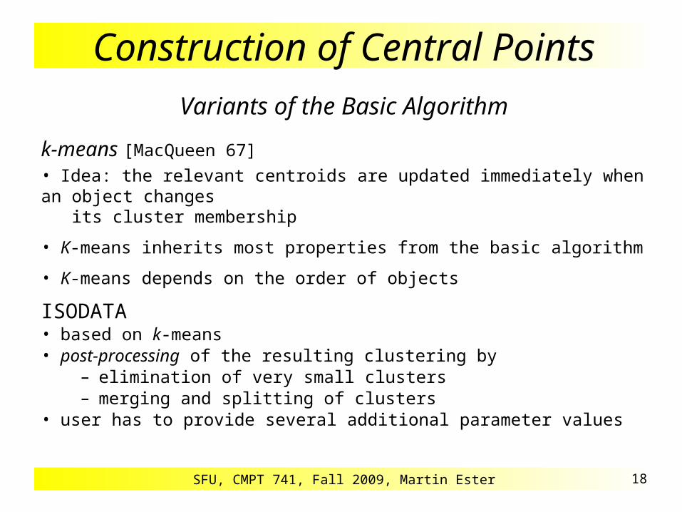
Variants of the Basic Algorithm
k-means [MacQueen 67]
• Idea: the relevant centroids are updated immediately when an object changes its cluster membership
• K-means inherits most properties from the basic algorithm
• K-means depends on the order of objects
ISODATA• based on k-means • post-processing of the resulting clustering by
– elimination of very small clusters– merging and splitting of clusters
• user has to provide several additional parameter values
SFU, CMPT 741, Fall 2009, Martin Ester 19
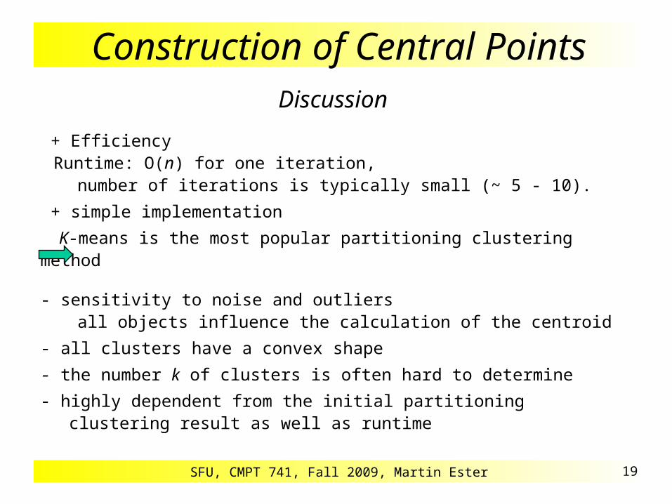
Construction of Central PointsDiscussion
+ Efficiency Runtime: O(n) for one iteration, number of iterations is typically small (~ 5 - 10).
+ simple implementation
K-means is the most popular partitioning clustering method
- sensitivity to noise and outliers all objects influence the calculation of the centroid
- all clusters have a convex shape
- the number k of clusters is often hard to determine
- highly dependent from the initial partitioning clustering result as well as runtime

SFU, CMPT 741, Fall 2009, Martin Ester 20
Selection of Representative Points
Basics [Kaufman & Rousseeuw 1990]
• Assumes only a distance function for pairs of objects
• Medoid: a representative element of the cluster (representative point)
• Measure for the costs (compactness) of a clusters C
• Measure for the costs (compactness) of a clustering
• Search space for the clustering algorithm: all subsets of cardinality k of the dataset D with |D|= n
runtime complexity of exhaustive search O(nk)
TD C dist p mC
p C
( ) ( , )
TD TD Ci
i
k
( )
1

SFU, CMPT 741, Fall 2009, Martin Ester 21
Selection of Representative Points
Overview of the AlgorithmsPAM [Kaufman & Rousseeuw 1990]
• greedy algorithm: in each step, one medoid is replaced by one non-medoid
• always select the pair (medoid, non-medoid) which implies the largest reduction of the costs TD
CLARANS [Ng & Han 1994]
two additional parameters: maxneighbor and numlocal
• at most maxneighbor many randomly chosen pairs (medoid, non-medoid) are considered
• the first replacement reducing the TD-value is performed
• the search for k „optimum“ medoids is repeated numlocal times

SFU, CMPT 741, Fall 2009, Martin Ester 22
Selection of Representative PointsAlgorithm PAM
PAM(dataset D, integer k, float dist)initialize the k medoids;TD_Update := while TD_Update 0 do
for each pair (medoid M, non-medoid N),calculate the value of TDNM;
choose the pair (M, N) with minimum value for TD_Update := TDNM TD;
if TD_Update 0 thenreplace medoid M by non-medoid N; record the set of the k current medoids as thecurrently best clustering;
return best k medoids;
SFU, CMPT 741, Fall 2009, Martin Ester 23
Selection of Representative Points
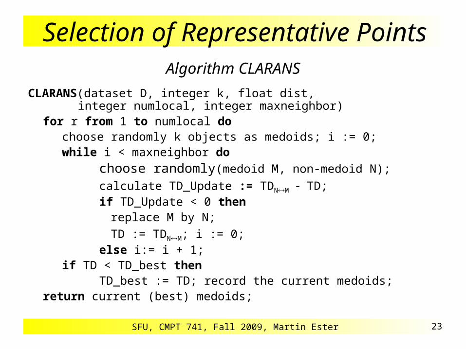
Algorithm CLARANS
CLARANS(dataset D, integer k, float dist, integer numlocal, integer maxneighbor)
for r from 1 to numlocal do choose randomly k objects as medoids; i := 0;while i < maxneighbor do
choose randomly(medoid M, non-medoid N);calculate TD_Update := TDNM TD;if TD_Update < 0 thenreplace M by N;
TD := TDNM; i := 0;else i:= i + 1;
if TD < TD_best thenTD_best := TD; record the current medoids;
return current (best) medoids;

SFU, CMPT 741, Fall 2009, Martin Ester 24
Selection of Representative Points
Comparison of PAM and CLARANSRuntime complexities• PAM: O(n3 + k(n-k)2 * #Iterations)
• CLARANS O(numlocal * maxneighbor * #replacements * n) in practice, O(n2)
Experimental evaluation
TD(CLARANS)
TD(PAM)
Quality Runtime
SFU, CMPT 741, Fall 2009, Martin Ester 25
Expectation Maximization
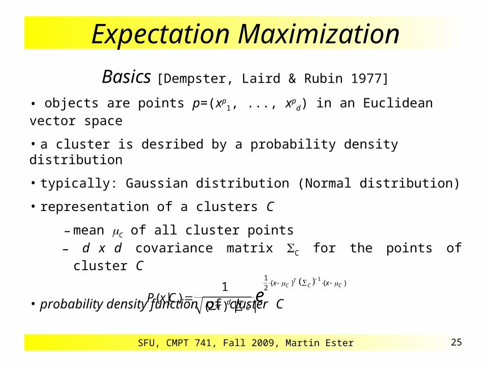
Basics [Dempster, Laird & Rubin 1977]
• objects are points p=(xp1, ..., xp
d) in an Euclidean vector space
• a cluster is desribed by a probability density distribution
• typically: Gaussian distribution (Normal distribution)
• representation of a clusters C
– mean C of all cluster points
– d x d covariance matrix C for the points of cluster C
• probability density function of cluster C
P x Cx x
dC
CT
C C
e( | )( ) | |
( ) ( )
1
21
1
2
SFU, CMPT 741, Fall 2009, Martin Ester 26
Expectation Maximization
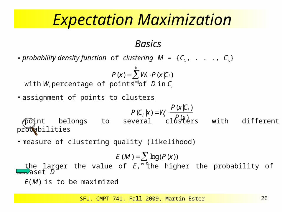
Basics• probability density function of clustering M = {C1, . . ., Ck}
with Wi percentage of points of D in Ci
• assignment of points to clusters
point belongs to several clusters with different probabilities
• measure of clustering quality (likelihood)
the larger the value of E, the higher the probability of dataset D
E(M) is to be maximized
P x W P x Ci i
i
k
( ) ( | )
1
P C x WP x C
P xi ii( | )
( | )
( )
E M P xx D
( ) log( ( ))

SFU, CMPT 741, Fall 2009, Martin Ester 27
Expectation MaximizationAlgorithm
ClusteringByExpectationMaximization (dataset D, integer k)
create an „initial“ clustering M’ = (C1’, ..., Ck’);
repeat // re-assignment
calculate P(x|Ci), P(x) and P(Ci|x) for each object x of D and each cluster Ci;
// re-calculation of clustering
calculate a new clustering M ={C1, ..., Ck} by re-calculating Wi, C and C for each i;
M’ := M;
until |E(M) - E(M’)| ;return M;

SFU, CMPT 741, Fall 2009, Martin Ester 28
Expectation Maximization
Discussion
• converges to a (possibly local) minimum
• runtime complexity:
O(n k * #iterations)
# iterations is typically large
• clustering result and runtime strongly depend on
– initial clustering
– „correct“ choice of parameter k
• modification for determining k disjoint clusters:
assign each object x only to cluster Ci with maximum P(Ci|x)

SFU, CMPT 741, Fall 2009, Martin Ester 29
Choice of Initial ClusteringsIdea• in general, clustering of a small sample yields good initial clusters• but some samples may have a significantly different distribution
Method [Fayyad, Reina & Bradley 1998]
• draw independently m different samples
• cluster each of these samples
m different estimates for the k cluster means
A = (A 1, A 2, . . ., A k), B = (B 1,. . ., B k), C = (C 1,. . ., C k), . . .
• cluster the dataset DB =
with m different initial clusterings A, B, C, . . .
• from the m clusterings obtained, choose the one with the highest clustering
quality as initial clustering for the whole dataset
A B C ...

SFU, CMPT 741, Fall 2009, Martin Ester 30
Choice of Initial Clusterings
Example
A2
A1
A3
B1
C1B2
B3
C2
C3
D1
D2
D3
whole dataset
k = 3
DB
from m = 4 samples
true cluster means

SFU, CMPT 741, Fall 2009, Martin Ester 31
Choice of Parameter k Method
• for k = 2, ..., n-1, determine one clustering each• choose the clustering with the highest clustering quality
Measure of clustering quality
• independent from k
• for k-means and k-medoid:
TD2 and TD decrease monotonically with increasing k
• for EM:
E decreases monotonically with increasing k

SFU, CMPT 741, Fall 2009, Martin Ester 32
Choice of Parameter k Silhouette-Coefficient [Kaufman & Rousseeuw 1990]
• measure of clustering quality for k-means- and k-medoid-methods• a(o): distance of object o to its cluster representative b(o): distance of object o to the representative of the „second-best“ cluster• silhouette s(o) of o
s(o) = -1 / 0 / +1: bad / indifferent / good assignment
• silhouette coefficient sC of clustering Caverage silhouette over all objects
• interpretation of silhouette coefficient
sC > 0,7: strong cluster structure,
sC > 0,5: reasonable cluster structure, . . .
s ob o a o
a o b o( )
( ) ( )
max{ ( ), ( )}
SFU, CMPT 741, Fall 2009, Martin Ester 33
Hierarchical Methods
Basics
Goal
construction of a hierarchy of clusters (dendrogram) merging clusters with minimum distance
Dendrograma tree of nodes representing clusters, satisfying the following properties:
• Root represents the whole DB.
• Leaf node represents singleton clusters containing a single object.
• Inner node represents the union of all objects contained in its corresponding subtree.
SFU, CMPT 741, Fall 2009, Martin Ester 34
Hierarchical Methods Basics
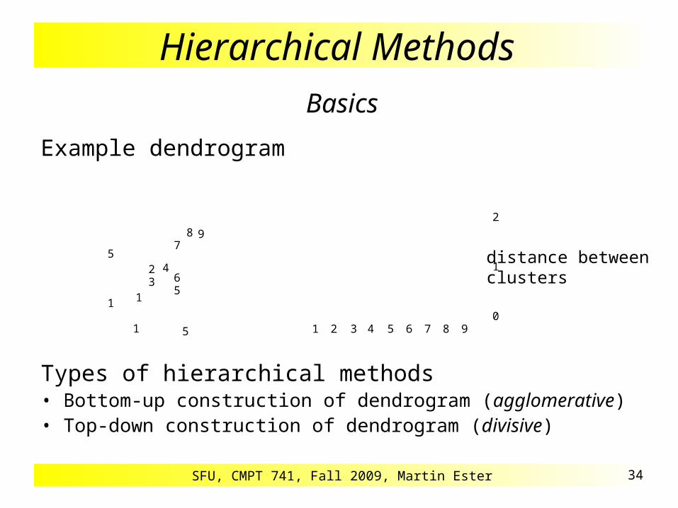
Example dendrogram
Types of hierarchical methods• Bottom-up construction of dendrogram (agglomerative)• Top-down construction of dendrogram (divisive)
1
1
5
5
132 4
65
78 9
1 2 3 4 5 6 7 8 90
1
2
distance betweenclusters

SFU, CMPT 741, Fall 2009, Martin Ester 35
Single-Link and Variants
Algorithm Single-Link [Jain & Dubes 1988]
Agglomerative Hierarchichal Clustering
1. Form initial clusters consisting of a singleton object, and computethe distance between each pair of clusters.
2. Merge the two clusters having minimum distance.
3. Calculate the distance between the new cluster and all other clusters.
4. If there is only one cluster containing all objects: Stop, otherwise go to step 2.
SFU, CMPT 741, Fall 2009, Martin Ester 36
Single-Link and Variants
Distance Functions for Clusters
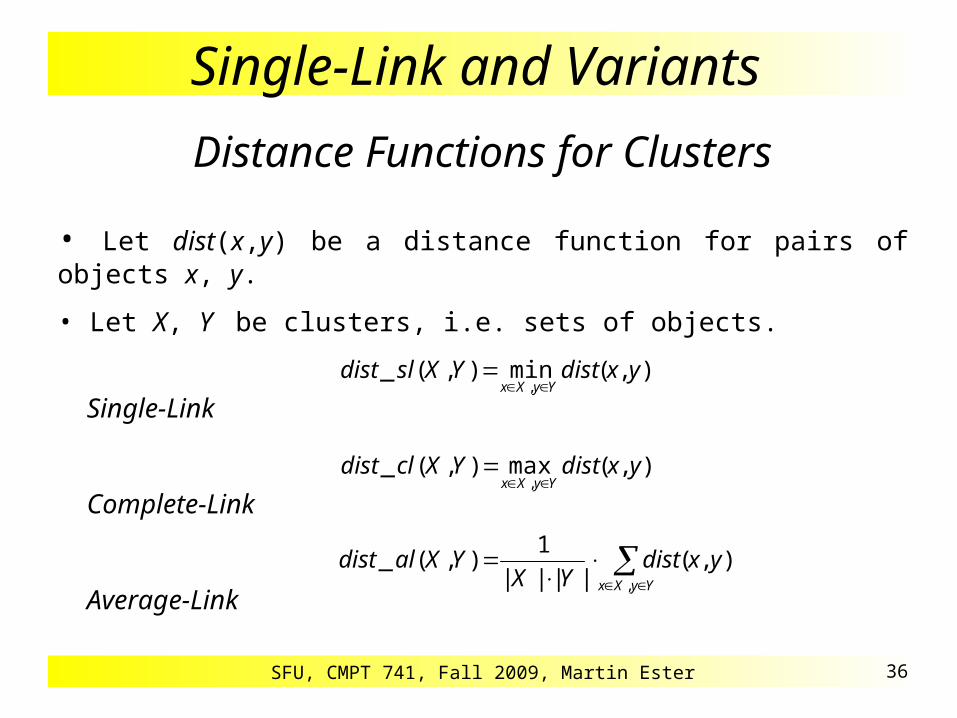
• Let dist(x,y) be a distance function for pairs of objects x, y.
• Let X, Y be clusters, i.e. sets of objects.
Single-Link
Complete-Link
Average-Link
),(min),(_,
yxdistYXsldistYyXx
),(max),(_,
yxdistYXcldistYyXx
YyXx
yxdistYX
YXaldist,
),(||||
1),(_

SFU, CMPT 741, Fall 2009, Martin Ester 37
Single-Link and Variants
Discussion
+ does not require knowledge of the number k of clusters
+ finds not only a „flat“ clustering, but a hierarchy of clusters (dendrogram)
+ a single clustering can be obtained from the dendrogram (e.g., by performing a horizontal cut)
- decisions (merges/splits) cannot be undone
- sensitive to noise (Single-Link) a „line“ of objects can connect two clusters
- inefficient runtime complexity at least O(n2) for n objects

SFU, CMPT 741, Fall 2009, Martin Ester 38
Single-Link and Variants CURE [Guha, Rastogi & Shim 1998]
• representation of a cluster partitioning methods: one object hierarchical methods: all objects• CURE: representation of a cluster by c representatives• representatives are stretched by factor of w.r.t. the centroid
detects non-convex clustersavoids Single-Link effect

SFU, CMPT 741, Fall 2009, Martin Ester 39
Density-Based Clustering Basics
Idea
• clusters as dense areas in a d-dimensional dataspace
• separated by areas of lower density
Requirements for density-based clusters
• for each cluster object, the local density exceeds some threshold
• the set of objects of one cluster must be spatially connected
Strenghts of density-based clustering
• clusters of arbitrary shape
• robust to noise
• efficiency

SFU, CMPT 741, Fall 2009, Martin Ester 40
Density-Based Clustering
Basics [Ester, Kriegel, Sander & Xu 1996]
• object o D is core object (w.r.t. D):
|N(o)| MinPts, with N(o) = {o’ D | dist(o, o’) }.
• object p D is directly density-reachable from q D w.r.t. and MinPts: p N(q) and q is a core object (w.r.t. D).
• object p is density-reachable from q: there is a chain of directly density-reachable objects between q and p.
p
q
p
q
border object: no core object,but density-reachable from other object (p)

SFU, CMPT 741, Fall 2009, Martin Ester 41
Density-Based Clustering
Basics
• objects p and q are density-connected: both are density-reachable from a third object o.
• cluster C w.r.t. and MinPts: a non-empty subset of D satisfying
Maximality: p,q D: if p C, and q density-reachable from p, then q C.
Connectivity: p,q C: p is density-connected to q.
SFU, CMPT 741, Fall 2009, Martin Ester 42
Density-Based Clustering
Basics
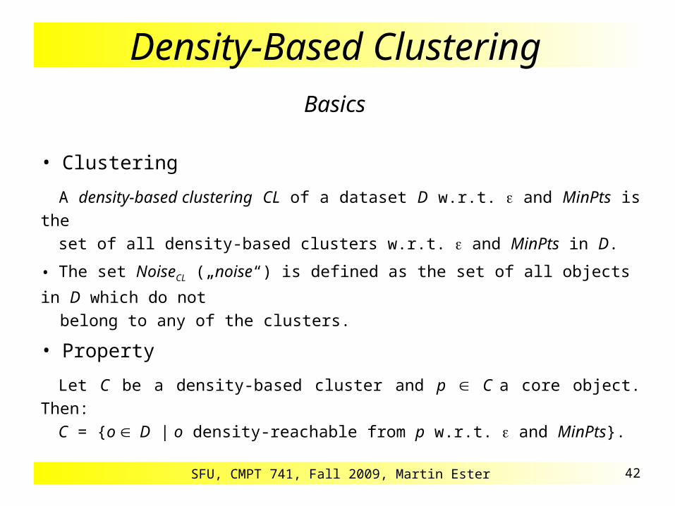
• Clustering
A density-based clustering CL of a dataset D w.r.t. and MinPts is the
set of all density-based clusters w.r.t. and MinPts in D.
• The set NoiseCL („noise“) is defined as the set of all objects in D which do not
belong to any of the clusters.
• Property
Let C be a density-based cluster and p C a core object. Then:
C = {o D | o density-reachable from p w.r.t. and MinPts}.
SFU, CMPT 741, Fall 2009, Martin Ester 43
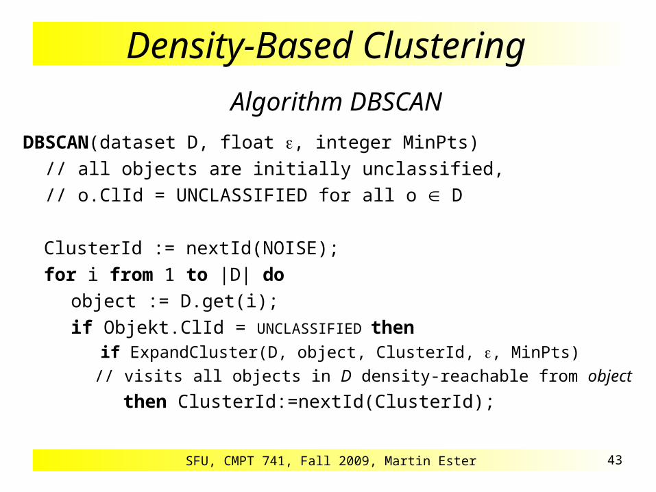
Density-Based Clustering Algorithm DBSCAN
DBSCAN(dataset D, float , integer MinPts) // all objects are initially unclassified,
// o.ClId = UNCLASSIFIED for all o D
ClusterId := nextId(NOISE);
for i from 1 to |D| do
object := D.get(i);
if Objekt.ClId = UNCLASSIFIED then if ExpandCluster(D, object, ClusterId, , MinPts) // visits all objects in D density-reachable from object
then ClusterId:=nextId(ClusterId);

SFU, CMPT 741, Fall 2009, Martin Ester 44
Density-Based Clustering
Choice of Parameters
• cluster: density above the „minimum density“ defined by andMinPts
• wanted: the cluster with the lowest density
• heuristic method: consider the distances to the k-nearest neighbors
• function k-distance: distance of an object to its k-nearest neighbor
• k-distance-diagram: k-distances in descending order
p
q
3-distance(p)
3-distance(q)

SFU, CMPT 741, Fall 2009, Martin Ester 45
Density-Based Clustering Choice of Parameters
Example
Heuristic Method
• User specifies a value for k (Default is k = 2*d - 1), MinPts := k+1.• System calculates the k-distance-diagram for the dataset and visualizes it.• User chooses a threshold object from the k-distance-diagram, = k-distance(o).
3-di
stan
ce
objects
threshold object o
first „valley“

SFU, CMPT 741, Fall 2009, Martin Ester 46
Density-Based Clustering
Problems with Choosing the Parameters
• hierarchical clusters• significantly differing densities in different areas of the dataspace • clusters and noise are not well-separated
A
B
C
D
E
D’
F
G
B’D1
D2
G1
G 2
G3
3-di
stan
ce
objects
A, B, C
B‘, D‘, F, G
B, D, E
D1, D2,G1, G2, G3
SFU, CMPT 741, Fall 2009, Martin Ester 47
Hierarchical Density-Based Clustering
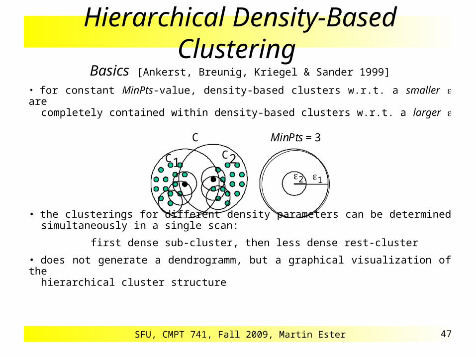
Basics [Ankerst, Breunig, Kriegel & Sander 1999]
• for constant MinPts-value, density-based clusters w.r.t. a smaller are completely contained within density-based clusters w.r.t. a larger
• the clusterings for different density parameters can be determined simultaneously in a single scan:
first dense sub-cluster, then less dense rest-cluster
• does not generate a dendrogramm, but a graphical visualization of the hierarchical cluster structure
MinPts = 3C
C1C2
2 1
SFU, CMPT 741, Fall 2009, Martin Ester 48
Hierarchical Density-Based Clustering
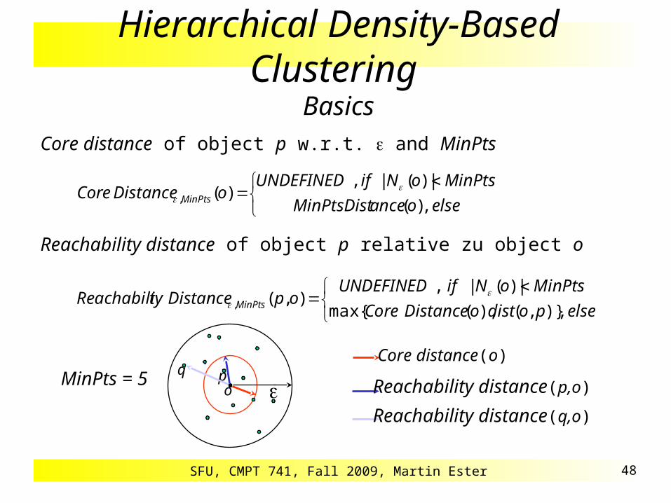
BasicsCore distance of object p w.r.t. and MinPts
Reachability distance of object p relative zu object o
MinPts = 5
elseoanceMinPtsDist
MinPtsoNifUNDEFINEDoDistanceCore MinPts ,)(
|)(|,)(,
elsepodistoDistanceCore
MinPtsoNifUNDEFINEDopDistancetyReachabili MinPts ,)},(),(max{
|)(|,),(,
opq
Core distance(o)
Reachability distance(p,o)
Reachability distance(q,o)

SFU, CMPT 741, Fall 2009, Martin Ester 49
Hierarchical Density-Based Clustering
Cluster Order
• OPTICS does not directly return a (hierarchichal) clustering, but orders the objects according to a „cluster order“ w.r.t. and MinPts
• cluster order w.r.t. and MinPts
– start with an arbitrary object
– visit the object that has the minimum reachability distance from the set of already visited objects
Core-distance
Reachability-distance 4
123 16 18
17
1
2
34
16 17
18
Core distanceReachability distance
cluster order

SFU, CMPT 741, Fall 2009, Martin Ester 50
Hierarchical Density-Based Clustering
Reachability Diagram• depicts the reachability distances (w.r.t. and MinPts) of all objects in a bar diagram
• with the objects ordered according to the cluster order
reac
habi
lity
dis
tanc
e
reac
habi
lity
dis
tanc
e
clusterorder

SFU, CMPT 741, Fall 2009, Martin Ester 51
Hierarchical Density-Based Clustering
Sensitivity of Parameters
1
2
3
MinPts = 10, = 10
1 2 3
MinPts = 10, = 5 MinPts = 2, = 10
1 2 3
1 2 3
“optimum” parameters smaller smaller MinPts
cluster order is robust against changes of the parameters
good results as long as parameters „large enough“

SFU, CMPT 741, Fall 2009, Martin Ester 52
Hierarchical Density-Based Clustering
Heuristics for Setting theParameters
• choose largest MinPts-distance in a sample or
• calculate average MinPts-distance for uniformly distributed data
MinPts• smooth reachability-diagram
• avoid “single-link” effect
... ... ... ...

SFU, CMPT 741, Fall 2009, Martin Ester 53
Hierarchical Density-Based Clustering
Manual Cluster Analysis
Based on Reachability-Diagram• are there clusters?
• how many clusters?
• how large are the clusters?
• are the clusters hierarchically nested?
Based on Attribute-Diagram• why do clusters exist?
• what attributes allow to distinguish the different clusters?
Reachability-Diagram
Attribute-Diagram

SFU, CMPT 741, Fall 2009, Martin Ester 54
Hierarchical Density-Based Clustering
Automatic Cluster Analysis-Cluster• subsequence of the cluster order
• starts in an area of -steep decreasing reachability distances
• ends in an area of -steep increasing reachability distances at approximately the same absolute value
• contains at least MinPts objects
Algorithm• determines all -clusters
• marks the -clusters in the reachability diagram
• runtime complexity O(n)

SFU, CMPT 741, Fall 2009, Martin Ester 55
Database Techniques for Scalable Clustering
Goal
So far• small datasets• in main memory
Now
• very large datasets which do not fit into main memory• data on secondary storage (pages)
random access orders of magnitude more expensive than in main memory
scalable clustering algorithms

SFU, CMPT 741, Fall 2009, Martin Ester 56
Use of Spatial Index Structures or Related Techniques
• index structures obtain a coarse pre-clustering (micro-clusters)
neighboring objects are stored on the same / a neighboring disk
block
• index structures are efficient to construct
based on simple heuristics
• fast access methods for similarity queries
e.g. region queries and k-nearest-neighbor queries
Database Techniques for Scalable Clustering

SFU, CMPT 741, Fall 2009, Martin Ester 57
Region Queries for Density-Based Clustering
• basic operation for DBSCAN and OPTICS: retrieval of -neighborhood for a database object o
• efficient support of such region queries by spatial index structures such as
R-tree, X-tree, M-tree, . . .
• runtime complexities for DBSCAN and OPTICS:
single range query whole algorithm
without index O(n) O(n2)
with index O(log n) O(n log n)
with random access O(1) O(n)
spatial index structures degenerate for very high-dimensional data

SFU, CMPT 741, Fall 2009, Martin Ester 58
Index-Based Sampling
Method [Ester, Kriegel & Xu 1995]
• build an R-tree (often given)• select sample objects from the data pages of the R-tree• apply the clustering method to the set of sample objects (in memory)• transfer the clustering to the whole database (one DB scan)
data pagesof an R-tree sample has similar
distribution as DB

SFU, CMPT 741, Fall 2009, Martin Ester 59
Index-Based Sampling
Transfer the Clustering to the whole Database
• For k-means- and k-medoid-methods:
apply the cluster representatives to the whole database (centroids, medoids)
• For density-based methods: generate a representation for each cluster (e.g. bounding box)
assign each object to closest cluster (representation)
• For hierarchichal methods: generation of a hierarchical representation (dendrogram or
reachability-diagram) from the sample is difficult
SFU, CMPT 741, Fall 2009, Martin Ester 60
Index-Based Sampling
Choice of Sample Objects
How many objects per data page? • depends on clustering method
• depends on the data distribution
• e.g. for CLARANS: one object per data page
good trade-off between clustering quality and runtime
Which objects to choose? • simple heuristics: choose the „central“ object(s) of the data page
SFU, CMPT 741, Fall 2009, Martin Ester 61
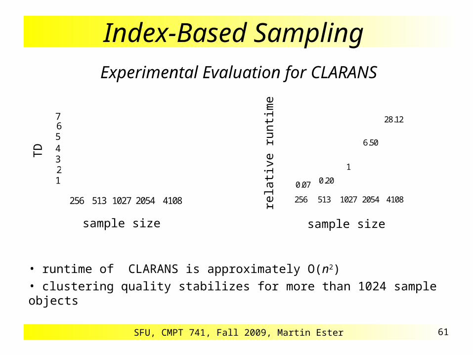
Index-Based Sampling Experimental Evaluation for CLARANS
• runtime of CLARANS is approximately O(n2)
• clustering quality stabilizes for more than 1024 sample objects
256 1027
45
2
7
1
3
6
2054 4108513
sample size
TD
256 513 1027
1
6.50
0.07
28.12
2054 4108
0.20
sample size
rela
tive
run
tim
e

SFU, CMPT 741, Fall 2009, Martin Ester 62
Data Compression for Pre-Clustering
Basics [Zhang, Ramakrishnan & Linvy 1996]
Method
• determine compact summaries of “micro-clusters” (Clustering Features)• hierarchical organization of clustering features
in a balanced tree (CF-tree)
• apply any clustering algorithm, e.g. CLARANS
to the leaf entries (micro-clusters) of the CF-tree
CF-tree
• compact, hierarchichal representation of the database
• conserves the “cluster structure”
SFU, CMPT 741, Fall 2009, Martin Ester 63
Data Compression for Pre-Clustering
Basics
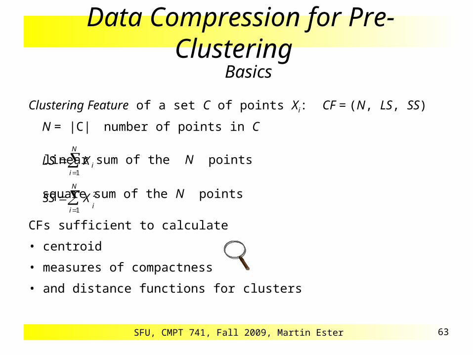
Clustering Feature of a set C of points Xi: CF = (N, LS, SS)
N = |C| number of points in C
linear sum of the N points
square sum of the N points
CFs sufficient to calculate
• centroid
• measures of compactness
• and distance functions for clusters
LS X ii
N
1
SS Xi
i
N
2
1
SFU, CMPT 741, Fall 2009, Martin Ester 64
Data Compression for Pre-Clustering
Basics
Additivity Theorem
CFs of two disjoint clusters C1 and C2 are additive:
CF(C1 C2) = CF (C1) + CF (C2) = (N1+ N2, LS1 + LS2, QS1 + QS2)
i.e. CFs can be incrementally calculated
Definition
A CF-tree is a height-balanced tree for the storage of CFs.

SFU, CMPT 741, Fall 2009, Martin Ester 65
Data Compression for Pre-Clustering
Basics
Properties of a CF-tree- Each innner node contains at most B entries [CFi, childi]
and CFi is the CF of the subtree of childi.
- A leaf node contains at most L entries [CFi].
- Each leaf node has two pointers prev and next. - The diameter of each entry in a leaf node (micro-cluster) does not exceed T.
Construction of a CF-tree
- Transform an object (point) p into clustering feature CFp=(1, p, p2).
- Insert CFp into closest leaf of CF-tree (similar to B+-tree insertions).
- If diameter threshold T is violated, split the leaf node.
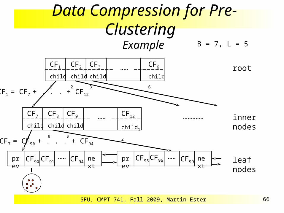
SFU, CMPT 741, Fall 2009, Martin Ester 66
Data Compression for Pre-Clustering
Example
CF1
child1
CF3
child3
CF2
child2
CF6
child6
CF7
child7
CF9
child9
CF8
child8
CF12
child12
CF90 CF91 CF94prev next CF95 CF96 CF99
prev next
B = 7, L = 5
root
inner nodes
leaf nodes
CF1 = CF7 + . . . + CF12
CF7 = CF90 + . . . + CF94

SFU, CMPT 741, Fall 2009, Martin Ester 67
Data Compression for Pre-Clustering
BIRCHPhase 1
• one scan of the whole database
• construct a CF-tree B1 w.r.t. T1 by successive insertions of all data objects
Phase 2
• if CF-tree B1 is too large, choose T2 > T1
• construct a CF-tree B2 w.r.t. T2 by inserting all CFs from the leaves of B1
Phase 3
• apply any clustering algorithm to the CFs (micro-clusters) of the leaf nodes of the resulting CF-tree (instead to all database objects)
• clustering algorithm may have to be adapted for CFs

SFU, CMPT 741, Fall 2009, Martin Ester 68
Data Compression for Pre-Clustering
Discussion
+ CF-tree size / compression factor is a user parameter
+ efficiency
construction of secondary storage CF-tree: O(n log n) [page accesses]
construction of main memory CF-tree : O(n) [page accesses]
additionally: cost of clustering algorithm
- only for numeric data Euclidean vector space
- result depends on the order of data objects
SFU, CMPT 741, Fall 2009, Martin Ester 69
Clustering High-Dimensional Data
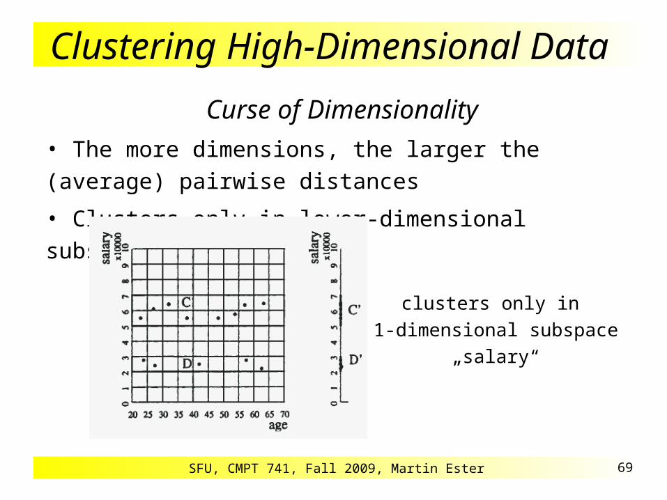
Curse of Dimensionality
• The more dimensions, the larger the (average) pairwise
distances
• Clusters only in lower-dimensional subspaces
clusters only in
1-dimensional subspace
„salary“
SFU, CMPT 741, Fall 2009, Martin Ester 70
Subspace Clustering CLIQUE [Agrawal, Gehrke, Gunopulos & Raghavan 1998]
• Cluster: „dense area“ in dataspace
• Density-threshold
region is dense, if it contains more than objects
• Grid-based approach
each dimension is divided into intervals
cluster is union of connected dense regions (region = grid cell)
• Phases
1. identification of subspaces with clusters
2. identification of clusters
3. generation of cluster descriptions

SFU, CMPT 741, Fall 2009, Martin Ester 71
Subspace Clustering
Identification of Subspaces with Clusters
• Task: detect dense base regions
• Naive approach:
calculate histograms for all subsets of the set of dimensions
infeasible for high-dimensional datasets (O (2d) for d dimensions)
• Greedy algorithm (Bottom-Up)
start with the empty set
add one more dimension at a time
• Monotonicity property
if a region R in k-dimensional space is dense, then each projection of R in
(k-1)-dimensional subspace is dense as well (more than objects)
SFU, CMPT 741, Fall 2009, Martin Ester 72
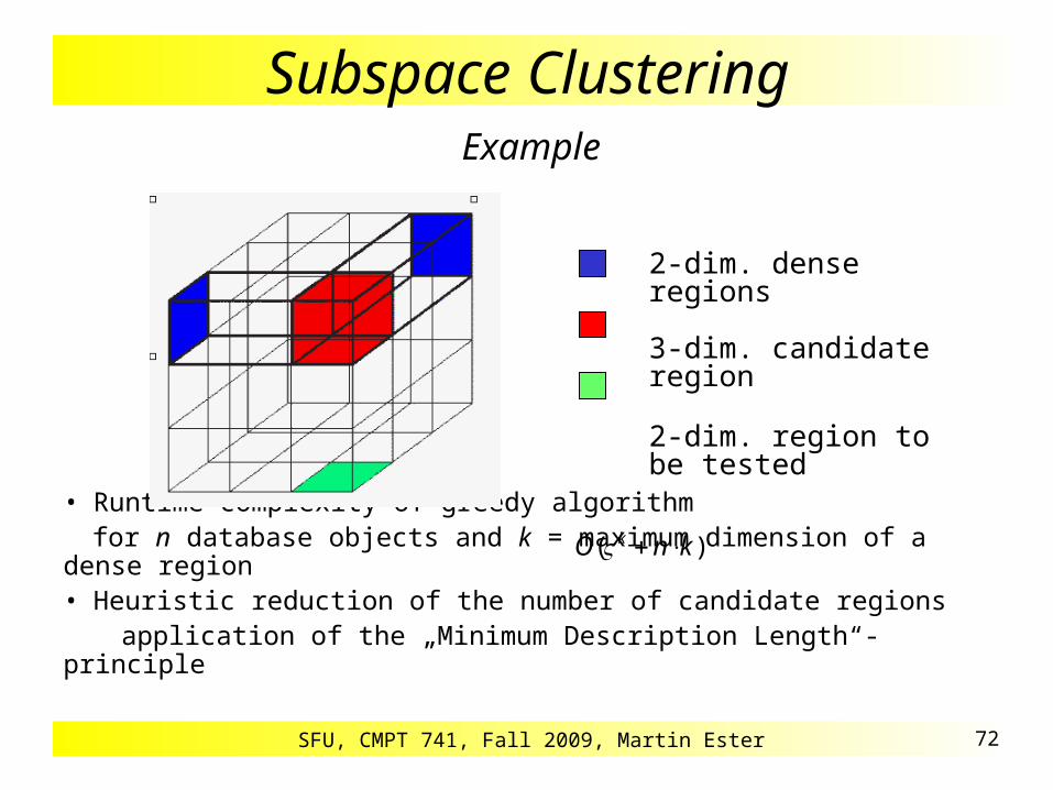
Subspace Clustering Example
• Runtime complexity of greedy algorithm for n database objects and k = maximum dimension of a dense region
• Heuristic reduction of the number of candidate regions application of the „Minimum Description Length“- principle
2-dim. dense regions
3-dim. candidate region
2-dim. region to be tested
O n kk( )

SFU, CMPT 741, Fall 2009, Martin Ester 73
Subspace Clustering
Identification of Clusters
• Task: find maximal sets of connected dense base regions
• Given: all dense base regions in a k-dimensional subspace
• „Depth-first“-search of the following graph (search space)
nodes: dense base regions
edges: joint edges / dimensions of the two base regions
• Runtime complexity
dense base regions in main memory (e.g. hash tree)
for each dense base region, test 2 k neighbors
number of accesses of data structure: 2 k n

SFU, CMPT 741, Fall 2009, Martin Ester 74
Subspace Clustering
Generation of Cluster Descriptions
• Given: a cluster, i.e. a set of connected dense base regions
• Task: find optimal cover of this cluster
by a set of hyperrectangles
• Standard methods
infeasible for large values of d
the problem is NP-complete
• Heuristic method
1. cover the cluster by maximal regions
2. remove redundant regions
SFU, CMPT 741, Fall 2009, Martin Ester 75
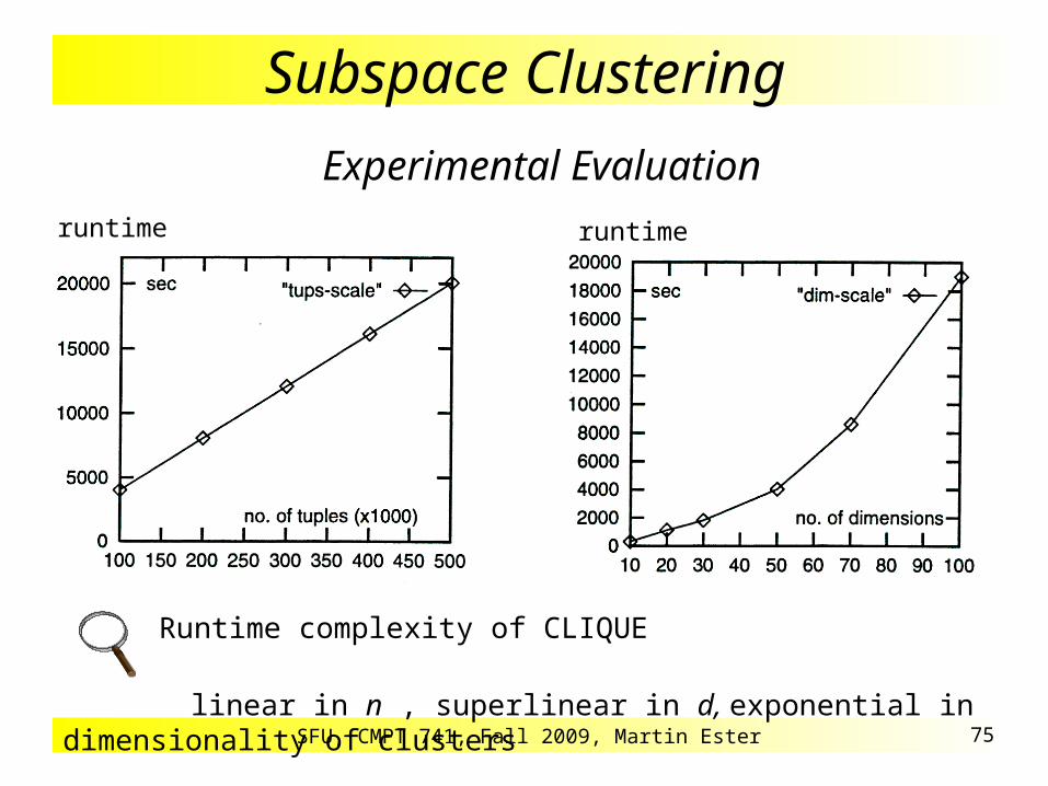
Subspace Clustering
Experimental Evaluation
Runtime complexity of CLIQUE
linear in n , superlinear in d, exponential in dimensionality of clusters
runtime runtime

SFU, CMPT 741, Fall 2009, Martin Ester 76
Subspace Clustering
Discussion
+ Automatic detection of subspaces with clusters
+ No assumptions on the data distribution and number of clusters
+ Scalable w.r.t. the number n of data objects
- Accuracy crucially depends on parameters and
single density threshold for all dimensionalities is problematic
- Needs a heuristics to reduce the search space
method is not complete

SFU, CMPT 741, Fall 2009, Martin Ester 77
Subspace Clustering Pattern-Based Subspace Clusters
Shifting pattern Scaling pattern(in some subspace) (in some subspace)
Such patterns cannot be found using existing subspace clustering methods since • these methods are distance-based • the above points are not close enough.
Attributes
Values
Attributes
Values
Object 1
Object 2Object 3
Object 1
Object 2
Object 3
SFU, CMPT 741, Fall 2009, Martin Ester 78
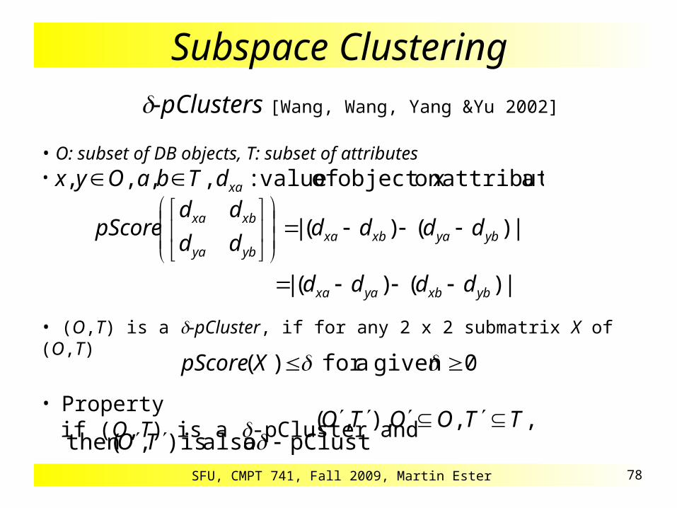
Subspace Clustering -pClusters [Wang, Wang, Yang &Yu 2002]
• O: subset of DB objects, T: subset of attributes •
• (O,T) is a -pCluster, if for any 2 x 2 submatrix X of (O,T)
• Propertyif (O,T) is a -pCluster and
a attributeon object x of value:,,,, xadTbaOyx
|)()(|
|)()(|
ybxbyaxa
ybyaxbxaybya
xbxa
dddd
dddddd
ddpScore
0given afor)( XpScore
pClustera alsois),(then TO,,),,( TTOOTO

SFU, CMPT 741, Fall 2009, Martin Ester 79
Subspace Clustering Problem
• Given , nc (minimal number of columns), nr (minimal number of rows), find all pairs (O,T) such that
• (O,T) is a pCluster•
•
• For pCluster (O,T), T is a Maximum Dimension Set if there does not exist
•
• Objects x and y form a pCluster on T iff the difference between the largest and smallest value in S(x,y,T) is below
nrO ||ncT ||
pCluster- a also is ),(such that TOTT
}|{),,( TaddTyxS yaxa
SFU, CMPT 741, Fall 2009, Martin Ester 80
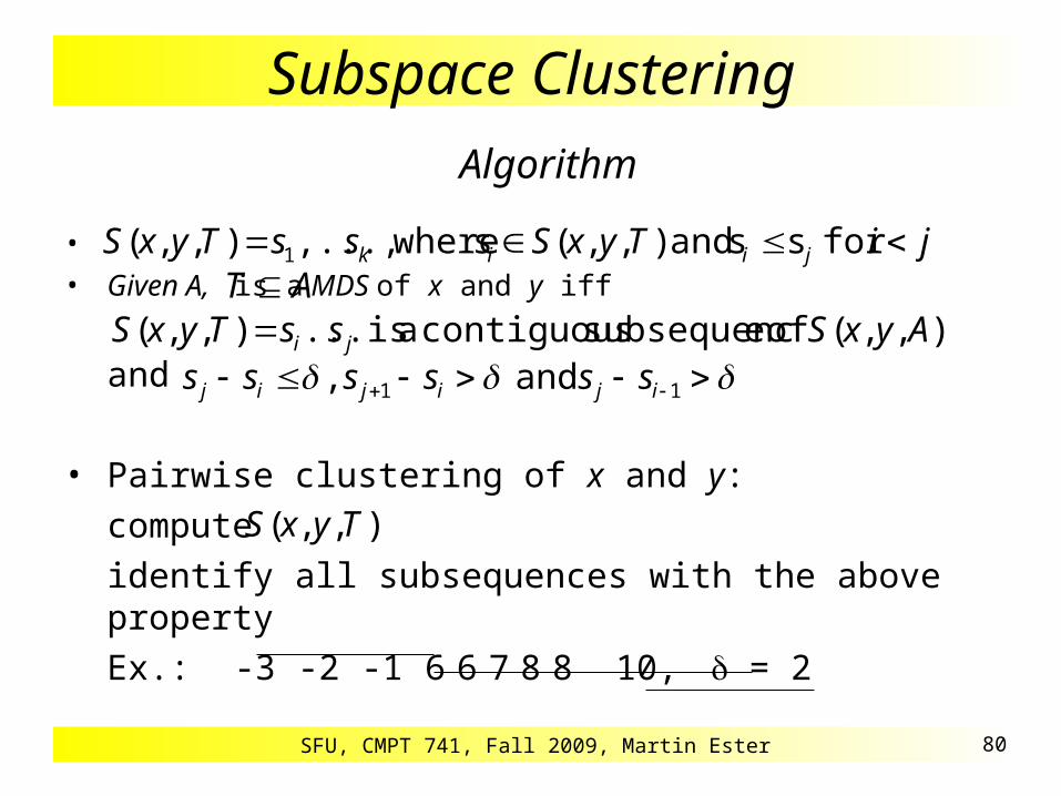
Subspace Clustering Algorithm
•
• Given A, is a MDS of x and y iff
and
• Pairwise clustering of x and y:
compute
identify all subsequences with the above property
Ex.: -3 -2 -1 6 6 7 8 8 10, = 2
11 and, ijijij ssssss
jiTyxSssTyxS jiik for ss and ),,(s where,...,),,( 1
AT ),,( of esubsequenc contiguous a is...),,( AyxSssTyxS ji
),,( TyxS
SFU, CMPT 741, Fall 2009, Martin Ester 81
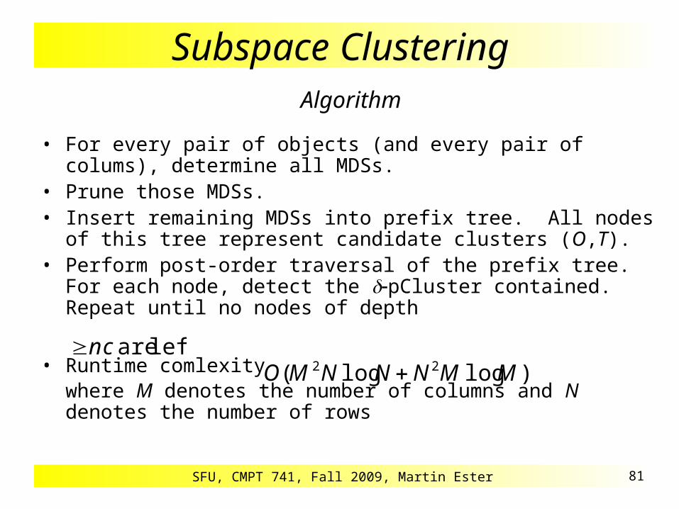
Subspace Clustering Algorithm
• For every pair of objects (and every pair of colums), determine all MDSs.
• Prune those MDSs.• Insert remaining MDSs into prefix tree. All nodes of this tree
represent candidate clusters (O,T).• Perform post-order traversal of the prefix tree. For each node,
detect the pCluster contained. Repeat until no nodes of depth
• Runtime comlexitywhere M denotes the number of columns and N denotes the number of rows
left. are cn)loglog( 22 MMNNNMO

SFU, CMPT 741, Fall 2009, Martin Ester 82
Projected Clustering PROCLUS [Aggarwal et al 1999]
• Cluster: Ci = (Pi, Di)
Cluster represented by a medoid
• Clustering:
k: user-specified number of clusters
O: outliers that are too far away from any of the clusters
l: user-specified average number of dimensions per cluster
• Phases1. Initialization2. Iteration3. Refinement
)dimensionsallof(setand DDDBP ii
},,,{ 1 OCC k
SFU, CMPT 741, Fall 2009, Martin Ester 83
Projected Clustering
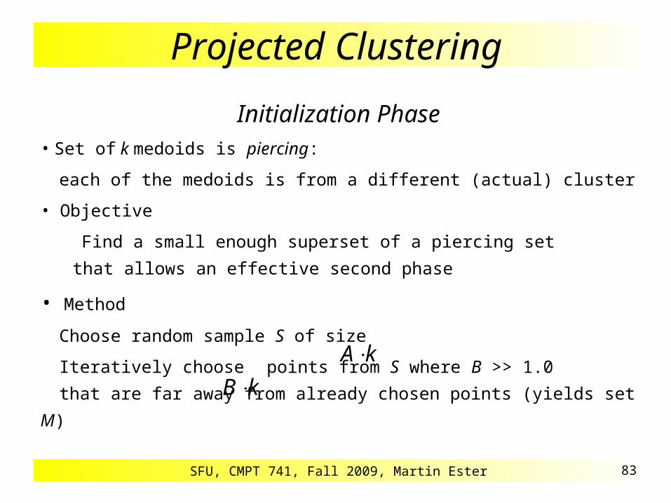
Initialization Phase• Set of k medoids is piercing:
each of the medoids is from a different (actual) cluster
• Objective
Find a small enough superset of a piercing set
that allows an effective second phase
• Method
Choose random sample S of size
Iteratively choose points from S where B >> 1.0
that are far away from already chosen points (yields set M)
kAkB

SFU, CMPT 741, Fall 2009, Martin Ester 84
Projected Clustering Iteration Phase
• Approach: Local Optimization (Hill Climbing)
• Choose k medoids randomly from M as Mbest
• Perform the following iteration step
Determine the „bad“ medoids in Mbest
Replace them by random elements from M, obtaining Mcurrent
Determine the best dimensions for the k medoids in Mcurrent
Form k clusters, assigning all points to the closest medoid
If clustering Mcurrent is better than clustering Mbest, then set Mbest to Mcurrent
• Terminate when Mbest does not change after a certain number of iterations
lk
SFU, CMPT 741, Fall 2009, Martin Ester 85
Projected Clustering
Iteration Phase
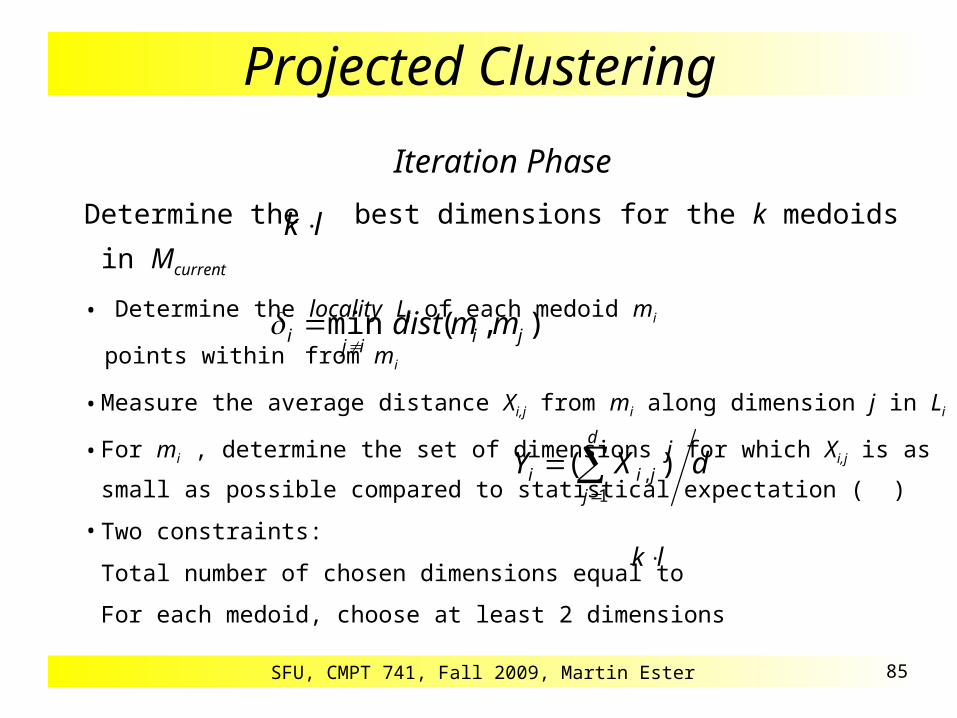
Determine the best dimensions for the k medoids in Mcurrent
• Determine the locality Li of each medoid mi
points within from mi
• Measure the average distance Xi,j from mi along dimension j in Li
• For mi , determine the set of dimensions j for which Xi,j is as small as possible
compared to statistical expectation ( )
• Two constraints:
Total number of chosen dimensions equal to
For each medoid, choose at least 2 dimensions
lk
),(min jiij
i mmdist
dXYd
jjii
1
, )(
lk

SFU, CMPT 741, Fall 2009, Martin Ester 86
Projected Clustering
Iteration Phase
Forming clusters in Mcurrent
• Given the dimensions chosen for Mcurrent
• Let Di denote the set of dimensions chosen for mi
• For each point p and for each medoid mi,
compute the distance from p to mi
using only the dimensions from Di
• Assign p to the closest mi
lk

SFU, CMPT 741, Fall 2009, Martin Ester 87
Projected Clustering Refinement Phase
• One additional pass to improve clustering quality
• Let Ci denote the set of points associated to mi at the end of the iteration phase
• Measure the average distance Xi,j from mi along dimension j in Ci
(instead of Li)
• For each medoid mi , determine a new set of dimensions Di applying the same
method as in the iteration phase
• Assign points to the closest (w.r.t. Di) medoid mi
• Points that are outside of the sphere of influence
of all medoids are added to the set O of outliers
),(min jiDij
i mmdisti
SFU, CMPT 741, Fall 2009, Martin Ester 88
Projected Clustering Experimental Evaluation
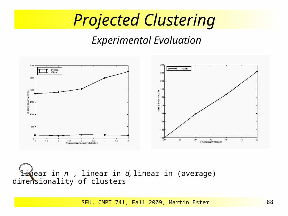
Runtime complexity of PROCLUS
linear in n , linear in d, linear in (average) dimensionality of clusters
SFU, CMPT 741, Fall 2009, Martin Ester 89
Projected Clustering Discussion
+ Automatic detection of subspaces with clusters
+ No assumptions on the data distribution
+ Output easier to interpret than that of subspace clustering
+ Scalable w.r.t. the number n of data objects, d of dimensions and the average
cluster dimensionality l
- Finds only one (of the many possible) clusterings
- Finds only spherical clusters
- Clusters must have similar dimensionalities
- Accuracy very sensitive to the parameters k and l
parameter values hard to determine a priori
SFU, CMPT 741, Fall 2009, Martin Ester 90
Constraint-Based Clustering Overview
• Clustering with obstacle objects When clustering geographical data, need to take into account physical obstacles such as rivers or mountains. Cluster representatives must be visible from cluster elements.
• Clustering with user-provided constraints Users sometimes want to impose certain constraints on clusters, e.g. a minimum number of cluster elements or a minimum average salary of cluster elements.
Two step method1) Find initial solution satisfying all user-provided constraints
2) Iteratively improve solution by moving single object to another cluster
• Semi-supervised clustering discussed in the following section

SFU, CMPT 741, Fall 2009, Martin Ester 91
Semi-Supervised Clustering Introduction
• Clustering is un-supervised learning
• But often some constraints are available from background knowledge
• In particular, sometimes class (cluster) labels are known for some of the records
• The resulting constraints may not all be simultaeneously satisfiable and are considered as soft (not hard) constraints
• A semi-supervised clustering algorithm discovers a clustering that respects the given class label constraints as good as possible

SFU, CMPT 741, Fall 2009, Martin Ester 92
Semi-Supervised Clustering A Probabilistic Framework [Basu, Bilenko & Mooney 2004]
• Constraints in the form of must-links (two objects should belong to the same cluster) and cannot-links (two objects should not belong to the same cluster)
• Based on Hidden Markov Random Fields (HMRFs)
• Hidden field L of random variables whose values are unobservable, values are from {1,. . ., K}:
• Observable set of random variables (X): every xi is generated from a conditional probability distribution
determined by the hidden variables L, i.e.
}{}{11
, iXiL xlN
i
N
i
Xx
ii
i
lxLX )|Pr()|Pr(

SFU, CMPT 741, Fall 2009, Martin Ester 93
Semi-Supervised Clustering Example HMRF with Constraints
Hidden variables: cluster labels
Observed variables: data points
K = 3

SFU, CMPT 741, Fall 2009, Martin Ester 94
Semi-Supervised Clustering Properties
• Markov property
Ni: neighborhood of lj, i.e. variables connected to lj via must/cannot-link
labels depend only on labels of neighboring variables• Probability of a label configuration L
N: set of all neighborhoods
Z1: normalizing constantV(L): overall label configuration potential function
V(L): potential for neighborhood Ni in configuration L
})|{|Pr(}){|Pr(: ijjiii NllllLli
))(exp(1
))(exp(1
)Pr(11
NN
N
i
iLV
ZLV
ZL

SFU, CMPT 741, Fall 2009, Martin Ester 95
Semi-Supervised Clustering Properties
• Since we have pairwise constraints, we consider only pairwise potentials:
• M: set of must links, C: set of cannot links• fM: function that penalizes the violation of must links, fC: function that penalizes the violation of cannot links
otherwise0
),( if),(
),( if),(
),(
where),),(exp(1
)Pr(1
Cxxxxf
Mxxxxf
jiV
iiVZ
L
jijiC
jijiM
i j

SFU, CMPT 741, Fall 2009, Martin Ester 96
Semi-Supervised Clustering Properties
•
• Applying Bayes theorem, we obtain
•
h
hXplxLXK
hXx
ii
i
clusteroftiverepresenta:
),()|Pr()|Pr(
h
1}{
),()),(exp(1
()|Pr( }{1
2hXpiiV
ZXL
K
hi j
)),(exp(
1),(
31
}{
Xxli
K
hi
ixD
ZhXp
ii lili xxD and between (distance) distortion :),(
SFU, CMPT 741, Fall 2009, Martin Ester 97
Semi-Supervised Clustering Goal
• Find a label configuration L that maximizes the conditional probability (likelihood) Pr(L|X)
• There is a trade-off between the two factors of Pr(L|X), namely Pr(X|L) and P(L)
• Satisfying more label constraints increases P(L), but may increasethe distortion and decrease Pr(X|L) (and vice versa)
• Various distortion measures can be usede.g., Euclidean distance, Pearson correlation, cosine similarity
• For all these measures, there are EM type algorithms minimizingthe corresponding clustering cost

SFU, CMPT 741, Fall 2009, Martin Ester 98
Semi-Supervised Clustering EM Algorithm
• E-step: re-assign points to clusters based on current representatives
• M-step: re-estimate cluster representatives based on currentassignment
• Good initialization of cluster representatives is essential
• Assuming consistency of the label constraints, these constraints are exploited to generate neighborhoods with representatives
• If < K, then determine K- additional representatives by random perturbations of the global centroid of X
• If > K, then K of the given representatives are selected that are maximally separated from each other (w.r.t. D)
SFU, CMPT 741, Fall 2009, Martin Ester 99
Semi-Supervised Clustering Semi-Supervised Projected Clustering [Yip et al 2005]
• Supervision in the form of labeled objects, i.e. (object,class label)pairs, and labeled dimensions, i.e. (class label, dimension) pairs
• Input parameter is k (number of clusters)
• No parameter specifying the average number of dimensions(parameter l in PROCLUS)
• Objective function essentially measures the average variance over all clusters and dimensions
• Algorithm similar to k-medoid
• Initialization exploits user-provided labels
• Can effectively find very low-dimensional projected clusters
SFU, CMPT 741, Fall 2009, Martin Ester 100
Outlier Detection
Overview
Definition
Outliers: objects significantly dissimilar from the remainder of the data
Applications
• Credit card fraud detection
• Telecom fraud detection
• Medical analysis
Problem
• Find top k outlier points

SFU, CMPT 741, Fall 2009, Martin Ester 101
Outlier Detection Statistical Approach
AssumptionStatistical model that generates data set (e.g. normal distribution)
Use tests depending on • data distribution
• distribution parameter (e.g., mean, variance)
• number of expected outliers
Drawbacks• most tests are for single attribute
• data distribution may not be known

SFU, CMPT 741, Fall 2009, Martin Ester 102
Outlier Detection Distance-Based Approach
Idea outlier analysis without knowing data distribution
DefinitionDB(p, t)-outlier:
object o in a dataset D such that at least a fraction p of the objects in D has a distance greater than t from o
Algorithms for mining distance-based outliers • Index-based algorithm
• Nested-loop algorithm
• Cell-based algorithm
SFU, CMPT 741, Fall 2009, Martin Ester 103
Outlier Detection
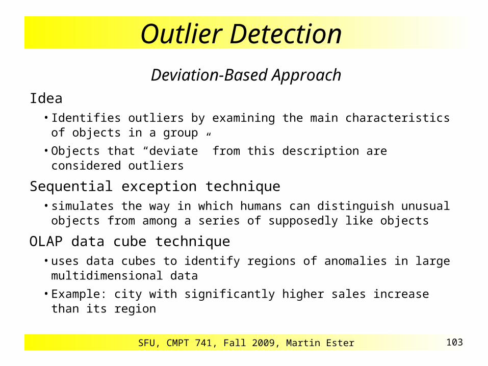
Deviation-Based ApproachIdea
• Identifies outliers by examining the main characteristics of objects in a group
• Objects that “deviate” from this description are considered outliers
Sequential exception technique • simulates the way in which humans can distinguish unusual objects from
among a series of supposedly like objects
OLAP data cube technique• uses data cubes to identify regions of anomalies in large multidimensional
data
• Example: city with significantly higher sales increase than its region


![SFU, CMPT 741, Fall 2009, Martin Ester 350 Graph Mining and Social Network Analysis Outline Graphs and networks Graph pattern mining [Borgwardt & Yan 2008]](https://img.pdfslide.net/doc/110x75/56649d265503460f949fcaac/sfu-cmpt-741-fall-2009-martin-ester-350-graph-mining-and-social-network.jpg)